08 Linear Programming - College of Charlestonhodgesh.people.cofc.edu/DSCI304/PPT/08 Linear Programming.pdf · Scheduling Shifts, Vehicles, Routing POM Applications. Lesson 08 –

Lesson 08 – Linear Programming

Copyright – Harland E. Hodges, Ph.D 08-1

08 - 1

Lesson 08Linear Programming

A mathematical approach to determine optimal (maximum or minimum) solutions to problems which involve restrictions on the variables involved.

08 - 2

Linear programming (LP) has been used to:

. establish locations for emergency equipment and personnel that minimize response time

. determine optimal schedules for planes

. develop financial plans

. determine optimal diet plans and animal feed mixes

. determine the best set of worker-job assignments

. determine optimal production schedules

. determine routes that will yield minimum shipping costs

. determine most profitable product mix

Linear Programming Applications

08 - 3

Aggregate planningProduction, Staffing

DistributionShipping

InventoryStock control, Supplier selection

LocationPlants or warehouses

Process managementStock cutting

SchedulingShifts, Vehicles, Routing

POM Applications



08 - 4

Type 2

How manyof each typedo I make to

maximize/minimize company

profits/costs?

A computer manufacturer makes two models of computers Type 1, and Type 2. The computers use many of the same components, made in the same factory by the same people and are stored in the same warehouse.

The Basic LP Question

Type 1

08 - 5

What Constrains What We Make?

Materials

Labor

Time

Cash

Storage Space

Shipping

Customer Requirements

Etc.

What Limits Us?

08 - 6

Objective (e.g. maximize profits, minimize costs, etc.)

Decision variables - those that can vary across a range of possibilities

Constraints - limitations for the decision variables

Parameters - the numerical values for the decision variables

Assumptions for an LP model. linearity - the impact of the decision variables is linear in both constraints and objective function

. divisibility - non-integer values for decision variables are OK

. certainty - values of parameters are known and are constant

. Non-negativity - decision variables >= 0

Components of Linear Programming



08 - 7

x = quantity of product 1 to producex = quantity of product 2 to producex = quantity of product 3 to produce

1

2

3

Decision Variables……………...

Objective Function (maximize profit)………………… 5x x x1 2 3+ +8 4

Subject ToLabor Constraint ……………………………..Material Constraint……………………………Product 1 Constraint………………………….Non-negativity Constraint……………………

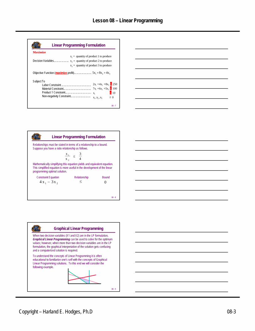
Linear Programming FormulationMaximizeMaximize

2x x x 2507x x x 100x 10x x x 0

1 2 3

1 2 3

1

1 2 3

+ + ≤+ + ≤

≤≥

4 86 5

, ,

08 - 8

Relationships must be stated in terms of a relationship to a bound. Suppose you have a ratio relationship as follows.

xx

34

1

2≤

Mathematically simplifying this equation yields and equivalent equation. This simplified equation is more useful in the development of the linear programming optimal solution.

Constraint Equation Relationship Bound4 3x x1 2− 0≤

Linear Programming Formulation

08 - 9

Graphical Linear ProgrammingWhen two decision variables (X1 and X2) are in the LP formulation, Graphical Linear Programming can be used to solve for the optimum values; however, when more than two decision variables are in the LP formulation, the graphical interpretation of the solution gets confusing and a computerized solution is required.

To understand the concepts of Linear Programming it is often educational to familiarize one’s self with the concepts of Graphical Linear Programming solutions. To this end we will consider the following example.



08 - 10

Example: A computer manufacturer makes two models of computers Type 1, and Type 2. The company resources available are also known. The marketing department indicates that it can sell what ever the company produces of either model. Find the quantity of Type 1 and Type 2 that will maximize company profits. The information available to the operations manager is summarized in the following table.

First we must formulate the Linear Programming Problem.

Graphical Linear Programming - Example

Per Unit Type 1 Type 2Amount Available

Profit $60 $50Assembly time (hr) 4 10 100Inspection time (hr) 2 1 22Storage space (cu ft) 3 3 39

08 - 11

x = quantity of Type 1 to producex = quantity of Type 2 to produce

1

2

Decision Variables

Objective Function (maximize profit) 60x x1 2+50

4x x 1002x x 223x x 39x x 0

1 2

1 2

1 2

1 2

+ ≤+ ≤+ ≤

≥

1013

,

Subject ToAssembly Time ConstraintInspection Time ConstraintStorage Space ConstraintNon-negativity Constraint


08 - 12

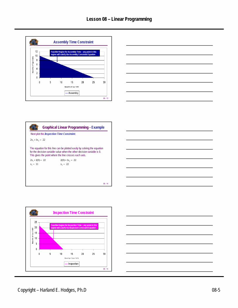
Next, we must plot each constraint (substituting the relationship with an equality sign). First plot the Assembly Time Constraint.

4x x 1001 2+ =10

The equation for this line can be plotted easily by solving the equation for the decision variable value when the other decision variable is 0. This gives the point where the line crosses each axis.4x (0) 100x 25

1

1

+ ==

10 4(0) x 100x 10

2

2

+ ==

10




08 - 13

Assembly Time Constraint

Feasible Region for Assembly Time – any point in this region will satisfy the Assembly Constraint Equation

08 - 14

Next plot the Inspection Time Constraint.


2x x 221 2+ =1


1

1

+ ==

1 2(0) x 22x 22

2

2

+ ==

1

08 - 15

Inspection Time Constraint

Feasible Region for Inspection Time – any point in this region will satisfy the Inspection Constraint Equation



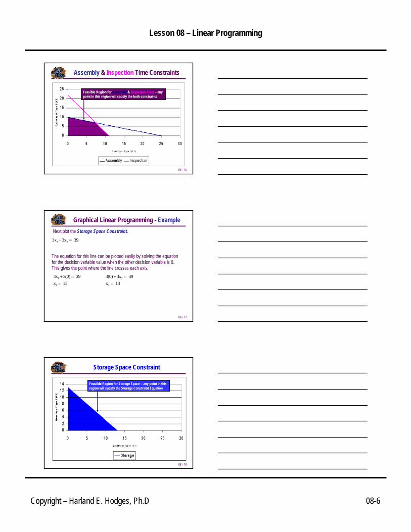
08 - 16

Assembly & Inspection Time Constraints

Feasible Region for Assembly & Inspection Time – any point in this region will satisfy the both constraints

08 - 17

Next plot the Storage Space Constraint.


3x x 391 2+ =3


1

1

+ ==

3 3(0) x 39x 13

2

2

+ ==

3

08 - 18

Storage Space Constraint

Feasible Region for Storage Space – any point in this region will satisfy the Storage Constraint Equation



08 - 19

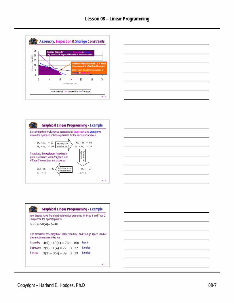
Assembly, Inspection & Storage Constraints

Feasible Region for Assembly, Inspection & Storage –any point in this region will satisfy all three constraints.

Optimum Profit (maximum) – is at one of the corner points of the feasible region.

In this case, it is at the intersection of Storage & Inspection

08 - 20

By solving the simultaneous equations for Inspection and Storage weobtain the optimum solution quantities for the decision variables.

2x x 223x x 39

1 2

1 2

+ =+ =

13

-6x x -663x x 39

1 2

1 2

− =+ =

33

Subtrac t the equatio ns

Multiply top equation by -3

-3x -27x 9

1

1

==

Substitute in one of the equations

2(9) x 22x 4

2

2

+ ==

1

Therefore, the optimum (maximum) profit is obtained when 9 Type 1 and 4 Type 2 computers are produced.


08 - 21

Now that we have found optimal solution quantities for Type 1 and Type 2 Computers, the optimal profit is

$74050(4)60(9) =+


4(9) 1002(9) 1(4) = 22 223(9) (4) = 39 39

+ = ≤+ ≤+ ≤

10 4 76

3

( )

The amount of assembly time, inspection time, and storage space used at these optimum quantities are

Assembly

Inspection

Storage

Slack

Binding

Binding



08 - 22

The previous example involved a Graphical Maximization Solution.

Graphical Minimization Solutions are similar to that of maximization with the exception that one of the constraints must be = or >=. This causes the feasible solution space to be away from the origin. The other difference is that the optimal point is the one nearest the origin.

We will not be doing any graphical minimization problems.

Graphical Minimization Solutions

08 - 23

Redundant Constraint - one which does not form a unique boundary of the feasible solution space.

Feasible Solution Space - a polygon.

Optimal solution - a point or line segment on the feasible solution space. The optimal solution is always at one of the corner points of the polygon. In the case that the optimal solution is a line segment of the polygon, any point on the line segment will yield the same optimum solution.

Other Linear Programming Terms

08 - 24

Binding Constraint -- one which forms the optimal corner point of the feasible solution space.

Surplus -- when the values of decision variables are substituted into a >= constraint equation and the resulting value exceeds the right side of the equation.

Slack -- when the values of decision variables are substituted into a <= constraint equation and the resulting value is less than the right side of the equation.

Other Linear Programming Terms



08 - 25

08 - 26

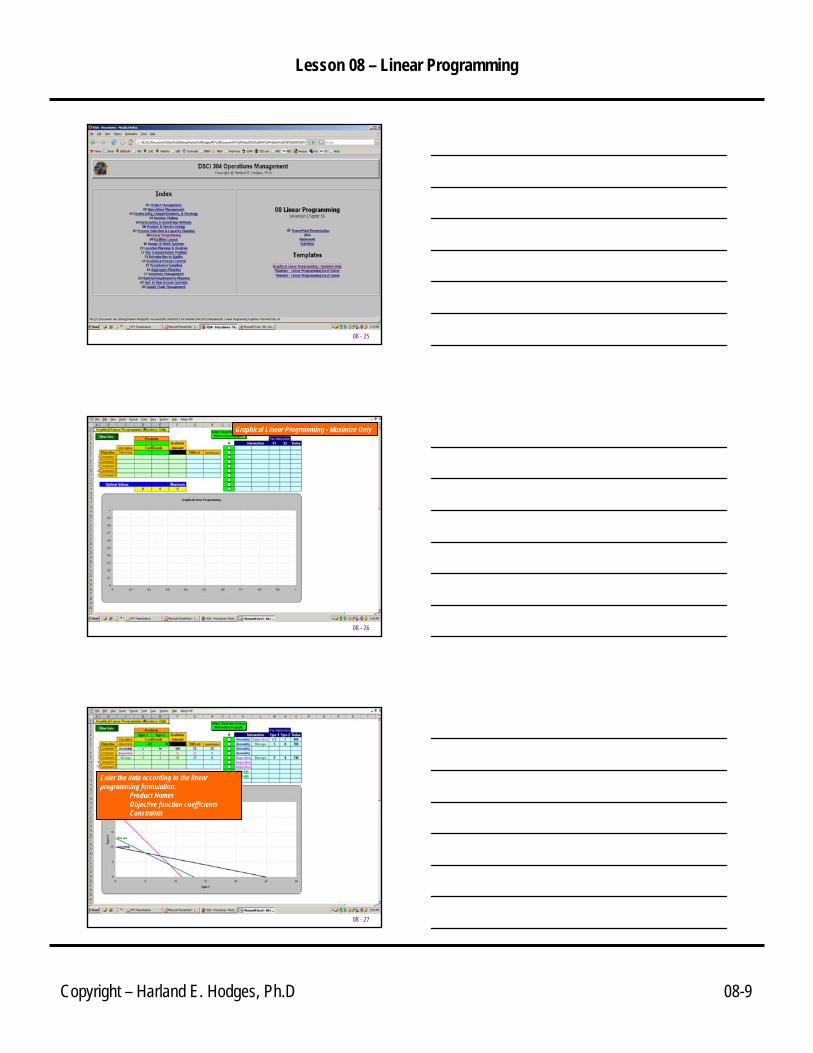
Graphical Linear Programming - Maximize Only

08 - 27

Enter the data according to the linear programming formulation:

Product Names Objective function coefficientsConstraints



08 - 28

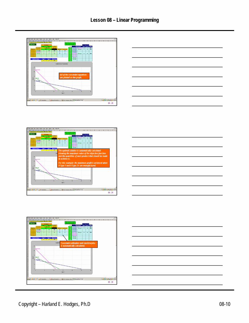
All of the constraint equations are plotted on the graph.

08 - 29

The optimal solution is automatically calculated showing the maximum value of the objective function and the quantities of each product that should be made to achieve it..

For this example: the maximum profit is achieved when 9 Type 1 and 4 Type 2’s are manufactured.

08 - 30

Constraint utilization and slack/surplus is automatically calculated.



08 - 31

Selecting the appropriate intersecting constraints shows the quantity points on the polygon where the objective function maximum is achieved.

08 - 32

EXCEL Solver LP - ExampleExample: A computer manufacturer makes two models of computers Type 1, and Type 2. The company resources available are also known. The marketing department indicates that it can sell what ever the company produces of either model. Find the quantity of Type 1 and Type 2 that will maximize company profits. The information available to the operations manager is summarized in the following table.

Per Unit Type 1 Type 2Amount Available

Profit $60 $50Assembly time (hr) 4 10 100Inspection time (hr) 2 1 22Storage space (cu ft) 3 3 39

08 - 33



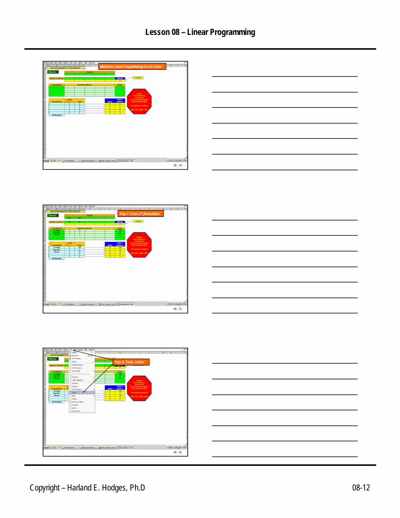
08 - 34

Maximize Linear Programming Excel Solver

08 - 35

Step 1: Enter LP formulation

08 - 36

Step 2: Tools, Solver



08 - 37

Step 3: Solve

08 - 38

Step 4: OK

08 - 39

The solution!Quantities of each product that yield the maximum objective.

Objective function maximum.

Constraint utilization and Slack/Suprlus



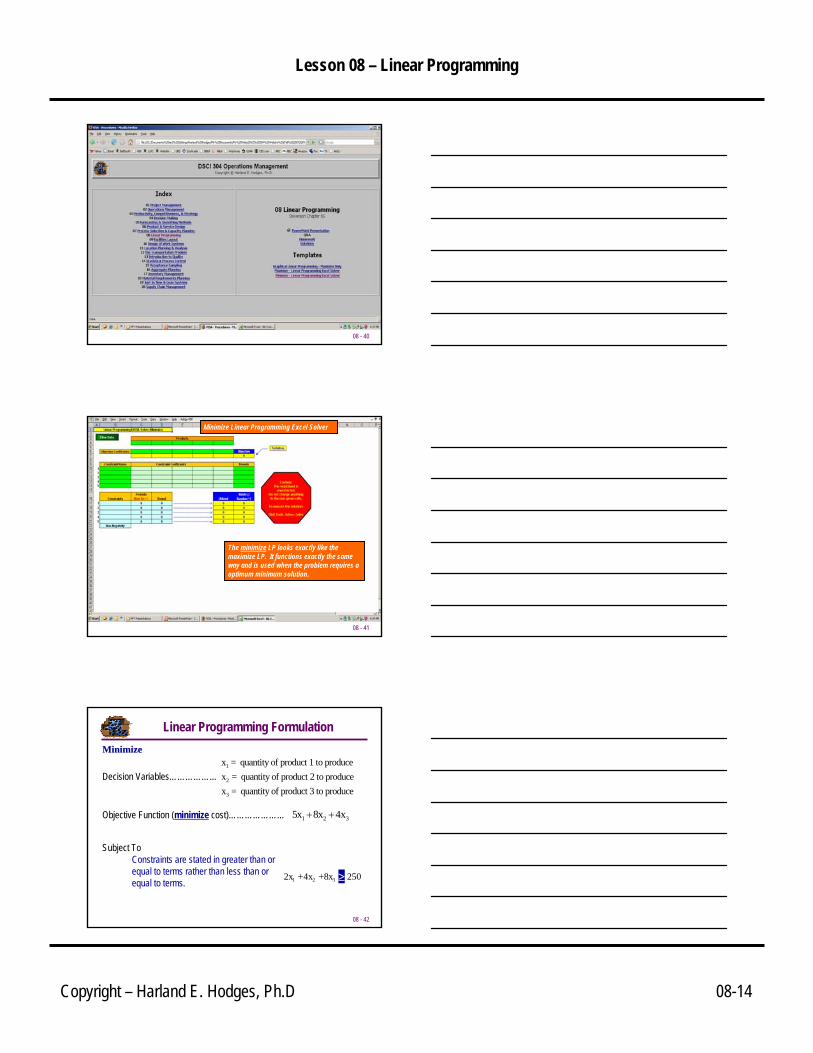
08 - 40

08 - 41

The minimize LP looks exactly like the maximize LP. It functions exactly the same way and is used when the problem requires a optimum minimum solution.

Minimize Linear Programming Excel Solver

08 - 42

x = quantity of product 1 to producex = quantity of product 2 to producex = quantity of product 3 to produce

1

2

3

Decision Variables……………...

Objective Function (minimize cost)………………… 5x x x1 2 3+ +8 4

Subject ToConstraints are stated in greater than or equal to terms rather than less than or equal to terms.

Linear Programming FormulationMinimizeMinimize

2x x x 2501 2 3+ + ≥4 8



08 - 43

EXCEL Solver LP Templates Read and understand all material in the chapter.

Discussion and Review Questions

Recreate and understand all classroom examples

Exercises on chapter web page

08 - 44

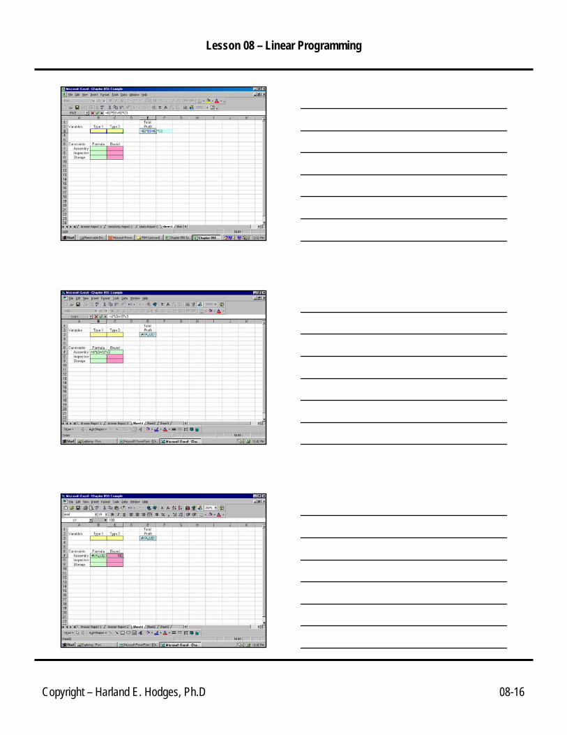
Appendix: EXCEL Solver DetailsIf you ever have to do your own solver, the following slides detail the steps in Excel you should follow.

08 - 45



08 - 46

08 - 47

08 - 48



08 - 49

08 - 50

08 - 51



08 - 52

08 - 53

08 - 54



08 - 55

08 - 56

08 - 57



08 - 58

08 - 59

08 - 60



08 - 61

08 - 62

08 - 63



08 - 64

Documents

08 Linear Programming - College of Charlestonhodgesh.people.cofc.edu/DSCI304/PPT/08 Linear Programming.pdf · Scheduling Shifts, Vehicles, Routing POM Applications. Lesson 08 –