AD-A239 802 / 0P PA11 IN 1 iiIIIliI 11,1 l 11E 1 II Is!t

Naval ucean mesearcn and Development ActivityJanuary 1990 Report 209

C)

An Analysis of Surface-duct Propagation LossModeling in SHARPS

DTIC^'ELECTE

AUG 22.1991130U

Robert W. McGirrNumerical Modeling DivisionOcean Acoustics and Technology Directorate

91-08367

Approved for public release; distribution is unlimited. Naval Ocean Research and Development Activity, Stennis Space Center,

Mississippi 39529-5004.

.. .91 8 20 112

717-7-7- T, V. 7 I

Foreword

The Fleet Numerical Oceanography Center is chartered to generate dailyforecasts of detection range for ASW sonar systems that operate in a widevariety of ocean environments. This report reviews the surface-duct propagationloss prediction capabilities of the Ship Helicopter Acoustic Range PredictionSystem. 0

W. B. Moseley J. B. Tupaz, Captain, USNTechnical Director Commanding Officer •

Executive Summary

The propagation submodels of the Ship Helicopter Acoustic RangePrediction System (SHARPS) are reviewed within the context of theireffectiveness in making accurate predictions for surface-duct environments.The surface-duct propagation loss calculations performed by SHARPS arebased on the submodels contained in Active RAYMODE. Fleet messages havebeen critical of SHARPS target detection range predictions for in-layerand cross-layer sonar-target geometries. A review is presented of thosecomputational methods-common to both Active and Passive RAYMODE-most likely to affect surface-duct predictions, and includes a summary of themain features of a surface-duct leakage subroutine found in one of the previousversions of Passive RAYMODE. A means of coupling surface-scattered energyinto the normal mode sum is reviewed. The possibility of "anomalous" surface-duct predictions is briefly addressed, and several ways to achieve improvedsurface-duct propagation loss predictions are recommended.

6 Acession For

FNTIS GRA&IDTIC TAB 0Uz Mru ou eed 0

justlf Icatio

By-Dstri butlon/_DI strlbutl on/

AvailabilitY CodesAvall and/oVv al i an o

i1st ISpecial

II

Acknowledgments

The author wishes to express his appreciation to Dr. David King of the NavalOcean Research and Development Activity (NORDA) for his technical reviewand helpful suggestions, to Mr. Curtis Favre for making model runs, and toLCDR Chris Hall of the Fleet Numerical Oceanography Center and Mr. EigoroHashimoto of NORDA (FNOC Liaison) for their encouragement and sup-port. The work reported herein was sponsored by FNOC's ASW TacticalSupport Division, Program Element 980101.

e 0

ii0

Contents

1. Introduction S

II. A Review of RAYMODE Model Physics 2A. Methods Used in Passive RAYMODE 2B. Original RAYMODE Integration 3C. Special High-frequency Integration 3D. Surface Reflection Loss 4

Ill. Surface-duct Propagation Modeling 4A. RAYMODE Surface-duct Model 4B. Characteristics of the Bilinear Profile Model 7

IV. Coupling of Surface Scattered Energy 9

V. Computational Artifacts 11

VI. Summary Remarks 12A. Conclusions 13B;.ecommendations 15

VII. References 16

Appendix A: Normal-mode and Multipath Expansion Forms 19

Appendix B: Special RAYMODE Integration 31

Appendix C: Breakdown of Phase Factor 37

Appendix D: Surface Reflection Loss Submodel 43

Appendix E: Complex Eigenvalues 47

Appendix F: Departure of n 2-linear Profile Model from Linearity 51

Appendix G: Modal Parameters for a C3-linear Duct 55

Appendix H: Bucker's Scattering Integrals 59

iii

'An Analysis of Surface-duct Propagation LossS'_JModeling in SHARPS

I. Introduction "streamlined" version of NISSM 11 (Weinberg, 1973;This report presents a qualitative assessment of the Kirby, 1982). From that point until 1986 this version

surface-duct propagation loss prediction capability of of the SHARPS model (then identified as SHARPSthe Ship-Helicopter Acoustic Range Prediction System III) underwent numerous upgrades.(SHARPS). SHARPS is used by the Fleet Numerical One of the major problems with both SHARPS 11Oceanography Center (FNOC) to generate daily fore- and SHARPS Ill centered on the surface-duct modelcasts of detection ranges for several operational sonar (based on the AMOS equations in both versions) and,systems. The Active RAYMODE model generates the in particular, the procedure used in defining the sonic-basic acoustic quantities used by the latest version of layer depth (for an amplification of this problem, seeSHARPS. The propagation loss subroutines of Active McGirr, 1983). The sonic layer depth problem wasRAYMODE were derived from Passive RAYMODE, never satisfactorily resolved. Indeed, the analyses ofthe latter being the new Navy standard propagation Renner and Kirby (1983) revealed that a pre-SHARPSloss model for range-independent ocean environ- profile-processing program occasionally yieldedments. Since the installation of Active RAYMODE in erroneous surface-duct parameters. This problem, inSHARPS, FNOC has received messages critical of combination with an overly simplified treatment of"anomalous" detection range predictions under certain surface-duct propagation, resulted in unacceptablysurface-duct conditions. large swings in detection range whenever the near-

Passive RAYMODE has been declared the Navy surface velocity gradients were exceptionally close tostandard propagation loss model for range-independent zero.ocean environments. As a consequence, all propagation Virtually the same problem exists with the newloss modules used in generating fleet prediction version of SHARPS, except that no special treatmentproducts had to be changed to meet the new standard. is given to surface-duct propagation. The near-surfaceThe decision was made that even though such changes propagation loss prediction problems that existed inwould be extremely costly, the costs were worth the previous versions of SHARPS were expected todesired result: commonality of all propagation loss disappear with the installation of Active RAYMODE.modules used in generating fleet prediction products. This supposition evidently emerged from expectationsThus, both the Active and the Passive versions of thatt.he "modal" character of the new propagationRAYMODE have been (or are being) installed at code would automatically take interduct coupling intoFNOC to provide the basic transmission loss calcula- account, thereby precluding any need for a surface-tions used in several fleet performance prediction duct submodel. These expectations were soon replacedsystems. by expressions of concern, however, once the message

The specific prediction system of interest here is traffic revealed the reality of the situation: the "normalSHARPS. This system was developed at FNOC in the node" method used in Active RAYMODE essentiallylate 1960s. In its original form, SHARPS was purely ignores the coupling of energy from one duct toempirical. In the early 1970s, SHARPS was completely another. Thus, the surface-duct problem persists, andrevised in an effort to incorporate the physics of under FNOC personnel once again find themselves trying towater sound. An attempt to use the original version respond to criticisms from the Fleet regarding theof the Navy Interim Surface Ship Model (NISSM) "same old problem."failed due to unacceptable run-times. A trimmed Essentially, recipients of SHARPS forecasts questionversion of NISSM, referred to simply as FAST NISSM in-layer and cross-layer detection range predictions. For(Watson and McGirr, 1972; McGirr, et al., 1972), was presumably well-defined surface ducts, predictedfinally installed for operational use in 1973. This detection ranges for both sonar and target in the ductcode (then identified as SHARPS II) had many are shorter than detection ranges predicted for sonarshortcomings and was replaced in 1977 by a in the duct and target below the duct. However,

0

on-board predictions for the same inputs yield the II. A Review of RAYMODE Modelopposite results. The first question is, were identical Physicsinputs used by both the ashore and the afloat prediction Passive RAYMODE was initially conceived in thesystems? The second question is, are both the ashore late 1960s by Leibiger (1968) and has evolved into aand the afloat implementations of the basic acoustic widely used propagation code. In essence, Leibigermodel (namely, Active RAYMODE) identical? replaces the single contour integral of the Fourier-

The first question can be answered only by Fleet Bessel solution to the reduced wave equation intoand FNOC personnel responsible for making the several integrals, each of which can be associated withpredictions. The second question, however, brings a family of rays. These integrals, which result fromup implementation issues. Both Active and Passive expanding the reciprocal of the Wronskian int, anRAYMODE are under configuration management and, infinite series, are then evaluated using an approximateas part of each software package, test cases are included normal-mode method if the number of modes is notfor verification. Presuming that the Active too large or otherwise using integration techniquesRAYMODE software was verified after being hard- more-or-less unique to RAYMODE. The advantageswired into the SHARPS "shell" and that a similar offered by RAYMODE over standard normal-modeverification procedure is faithfully followed after treatments are two-fold. First, the computationalinstallation in each system afloat, the logical course load does not significantly increase with increasingof action entails comparing surface-duct predictions frequency, as is the case with normal-mode models.generated by ashore and afloat version of Active Second, the solution is partitioned into componentsRAYMODE against high-confidence control models. that give rise to plausible geometrical interpretationsIf acceptable agreement is not obtained by either similar to those available from methods based strictlyversion, then the only recourse is to analyze the physics on ray acoustics.contained in Active RAYMODE that deals with The propagation-loss algorithms used in Activesurface-duct environments. RAYMODE essentially form a subset of those used

The verification procedure alluded to above may in Passive RAYMODE. As a consequence, Activenot uncover "bugs" peculiar to implementations on RAYMODE users are concerned about the lossspecific machines or operating systems. Steps have in accuracy that could result from calculationsbeen taken by both the developing agency, the Naval restricted to the high-frequency algorithms of PassiveRAYMODE. Concerns of the same sort also pertainUnderwater Systems Center (NUSC), and the organiza- RAYMODE , since numerous asuptin

tion responsible for configuration management, Naval and approximations havsne nume in an effort to

Oceanographic Office (NA VOCEANO), to ensure that obtain fast execution times. The focus here is on thosethere is no machine/operating-system dependency. The aspects of RAYMODE that potentially impact surface-RAYMODE codes delivered to the Naval Ocean duct predictions.Research and Development Activity (NORDA) wereprogrammed in strict FORTRAN 77, which should be A. Methods Used in Passive RAYMODEfree of any such dependencies. Nonetheless, there is Certain documents (Leibiger, 1968, 1971;always the possibility that a model which generates Deavenport, 1978; Davis and Council, 1985a, 1985b)acceptable results on the HP-9020/UNIX will not, present various aspects of the model physics. The textfor some cases, generate identical results on a VAX by DiNapoli and Deavenport (1979) is an excellentrunning VMS. Even though there may be some ques- reference on contemporary propagation modeling intions regarding verification, which are presumably general, and also presents a brief discussion ofbeing addressed by the various software firms involved, RAYMODE. Those documents written by Davis andthe purpose of the effort reported herein is to uncover Council are the most complete, although the sectionsweaknesses in the Active-RAYMODE model with that address the special surface-duct treatment do not

regard to surface-duct predictions. apply to the most recent version of Passive •The report is broken down into four major sections. RAYMODE, since the surface-duct module is not

ion I included in the latest version. Moreover, this surface-pysco deviews those mighhaspetso e eariMo duct treatment evidently has never been considered forphysics modeling that might have some bearing on inclusion in Active RAYMODE.surface-duct predictions. Section III addresses surface- The steps leading to the RAYMODE versions ofduct propagation modeling problems in general. normal-mode and multipath expansion solutions areSection IV examines the impact of neglecting surface developed in Appendix A. Much of the materialscattered energy. Section V illustrates jump discon- presented in Appendix A parallels the Passivetinuities that are common to methods based on hybrid RAYMODE documentation of Davis and Councilsolutions, and Section VI closes the report with (1985b). Readers who are interested in understandingsummary remarks and recommendations. the model physics should peruse all of the references.

20

For surface-duct paths, three RAYMODE methods then discarded in favor of the method outlined incan be applied to solve the multipath expansion Appendix B.integral, although the surface-duct option offered in a Leibiger (1971) demonstrates the relationshipprevious version of RAYMODE essentially represents between the stationary-phase "formula" and thea fourth RAYMODE method. The other three methods standard ray-acoustical expression. In an earlier reportare (1) numerical integration based on the fast, Fourier (Leibiger, 1968), he demonstrates that the existence oftransform (FFT); (2) the original RAYMODE inte- a point of stationary phase implies the existence of agration (ORI) method; and (3) a special high-frequency ray trajectory connecting the source and the receiver.integration (HFI) method. If the user does not select a The ORI method, as presented in Appendix B,particular method, then the program selects one. suggests the not entirely implausible possibility that theFor frequencies less than 3000 Hz, either of the first amplitude and phase factors do not necessarily accedetwo methods is selected, depending on estimated to conditions generally assumed extant in justifying theexecution time for each method. If the best option is application of stationary-phase methods. These mattersthe FFT method, but aliasing is anticipated, then the are discussed in Appendix C. Even when the evaluationORI method is used instead. For frequencies greater occurs at an end point, a stationary phase analysis canthan 3000 Hz, the special HFI method is seletted. The be used successfully to determine asymptotic behavior.methods of primary interest here are the original A precise assessment of the impact of asymptoticRAYMODE integration method and the special HFI behavior is beyond the scope of this effort, but as amethod. The special surface-duct treatment that practical matter, in any problem where a functionLeibiger applied in a previous version of RAYMODE is to be approximated, some a priori upper bound isis discussed in Section I1. The ORI and HFI methods placed on the tolerable error. A perusal of the computerare discussed in the next two subsections. code indicates that Leibiger has taken precautionary

steps to circumvent serious problems.B. Original RAYMODE Integration Some hint about the magnitude of error attributable

The general form of the RAYMODE multipath to the ORI method can be gleaned from Bartberger'sexpansion* integral (see Eq. (A38) in Appendix A) is (1981) evaluation of a previous version of Passive

RAYMODE. Bartberger notes that differences between1(k., kb) =113(k) exp{-i[kr + or(k)I dk, (1) the normal-mode method and the ORI method (which

P may have been altered since) can be significant forwhere the limits of integration extend from ka to kb. coherently summed outputs but appear to be minorAn approach often used in the evaluation of integrals for incoherently summed outputs. Discontinuousof this form is the method of stationary phase. This jumps that are created when the method of solutionmethod is summarized in Appendix B. switches from one form to another are briefly examined

Leibiger interrupts the stationary-phase analytical in Section IV.process and does not actually proceed to the final Leibiger (1971) notes that his particular stationary-formula (see Eq. (B51) of Appendix B). The reason phase treatment avoids certain problems that can

for this circumvention is that the conditions required develop as the acoustic frequency increases. At a high

to achieve the final step may not, for all frequencies enough frequency, the ORI method is supplemented

of interest, be met. An acceptable application of the by a special high frequency integration HFI approach.

formula requires that the function in the exponent,h(k), be multiplied by a large constant. The constant . Special High-frequency Integrationin the development as presented in Appendix B is unity. Keep in mind that a derivation of the high-frequencyThe argument of the phase function can be expressed procedure has not been documented by the .modelas, for example, k o [kr/k + a(k)/k,], and the developer, so the only information available is the briefvariable of integration transformed to k/k o, where ko description given by Davis and Council (1985b), and( = 2nf/C ) is some reference wavenumber. Thus, the computer code. The main features of this technique

the stated condition is met for high frequencies. are presented in Appendix B.

For low frequencies, the limits of integration must A perusal of the computer code for details on how

be confined to a relatively small interval, where the HFI procedure is implemented reveals that the Airy

(hopefully) the resulting integral yields an accurate integral is approximated by a polynomial of degree six

estimate. Early work by Leibiger (1968) indicates that when the argument has magnitude less than five, and

the stationary-phase formula was initially exploited and by the inverse square of the argument otherwise. Thisparticular form of asymptotic representation seemsrather crude, although quite possibly justified. The

*For an elementary interpretation of this technique consult polynomial approximation appears to be a truncatedSect. 35 in the text by Brekhovskikh (1980). power series expansion, which probably can be

10 3

improved upon by using an economized rational except at the surface and the bottom. In the specialpolynomial approximation instead, treatment accorded surface ducts, generalized Wentzel-

Kramers-Brillouin (WKB) reflection coefficients areD. Surface Reflection Loss introduced. These reflection coefficients are then used

RAYMODE surface reflection loss calculations are in constructing complex eigenvalues, where eachbased on an ad hoc adaptation of results derived in imaginary component corresponds to an exponentialpart from theoretical considerations and in part from loss of energy with range. Thus, for a source locatedexperimental data (Marsh and Schulkin, 1962). A within the duct, WKB modes lose some of their energysummary of this submodel is presented in Appendix D. at each turning point, where the lost energy is

transmitted into the region below the layer depth.Similarly, modes excited by a source located in (he 0

III. Surface-duct Propagation Modeling negative-gradient region transfer some of their energyThis section addresses several more or less to waves that propagate within the duct. This

independent aspects of modeling propagation loss for procedure, if added to the present version of Activesurface-duct environments. One of the working RAYMODE, should yield improved estimates ofhypotheses upon which this report is based is that the surface-duct propagation. To have any impact atsurface-duct model used in the 1983 version of frequencies above, say, 3 kHz, the maximum numberRAYMODE can, with suitable modifications, yield of modes would have to be extended to about 50. Thus,improved surface-duct predictions if incorporated into questions naturally arise pertaining to run-time andthe latest versions of the RAYMODE codes. Modifica- accuracy required in the determination of the complextions are necessary for two reasons: there appear to eigenvalues.be errors in the computer code and some means The only documentation on the basis for this specialshould be incorporated to account for the coupling of surface-duct procedure is the brief account presented •surface-scattered energy into the below-layer region. by Davis and Council (1985b). (The generalized WKBThis latter topic is addressed in Section IV. reflection coefficient procedure is described in the

The RAYMODE special surface-duct algorithms article by Murphy and Davis, 1974) The modificationsalluded to are discussed in Section A. Section B presents to the mode sum depend on source-receiver geometry.some characteristics of the two-segment n 2-linear When both the source depth (z,) and the receivervelocity profile model, which forms the basis of the depth (z,) are less than the layer depth (zL), the modesurface-duct module used in the latest versions of sums are applicable using appropriate reflectionFACT and ASTRAL. This approach to the problem coefficients at the turning points. The upper turninghas both advantages and disadvantages. A procedure point in this case is the surface; therefore, R.that was successfully used in the 1960s is reviewed, and corresponds to the surface reflection coefficientseveral detracting features of the n2-linear model are (discussed in Appendix A). At the lower turning pointdiscussed. depth, say, z,, R, is replaced by RAs(z,), a generalized

WKB reflection coefficie.it. The subscript, AB,A. RAYMODE Surface-duct Model indicates the sense of direction associated with theThe normal-mode sum used in Active RAYMODE coefficient, where A stands for above-layer and BThe orml-mde sm ued n AciveRAYODE stands for below-layer. Details pertaining to the

is possibly adequate to handle range-invariant, shallow- calculation of this coefficient, along with the corres-water ducts. For deep-ocean profiles that contain c on f this coefficient, aepresentedcr nes

multiple ducts, there is no provision for cross-channel ponding transmission coefficient, are presented in

coupling. Also, the mode sum is limited to a maximum subsequent paragraphs.When both the source and the receiver are situatedof 10 propagating modes, so for frequencies above below the layer depth, the reflection coefficient at theabout 3 kHz most ducts are likely to be handled by upper turning point is replaced by RsA(zu), which is

the HFI method. In many normal-mode codes, the similar tO RAn( ) for the in-layer case, but where

modes (eigenvalues) are determined by numerical the above-layer and below-layer parameters are

integration over the entire water column. Some codesuse iterative procedures to solve the characteristic interchanged. The lower turning point is assumed to

equation. In either case, interchannel coupling effects be at depth; therefore, R1 is assumed to have aare automatically included. The simplified procedure magnitude of I and a phase of -n/2.used in Active RAYMODE, as it stands, cannot For the cross-layer case, say, z, < ZL and z, > ZL,address this type of coupling. Leibiger takes a different approach. Instead of

The 1983 version of Passive RAYMODE includes reflection coet'ficients, the amplitude factors arethe option of a special treatment of the normal-mode multiplied by a transmission coefficient. Thus, energymethod when applied to surface ducts. In the standard that would otherwise be considered trapped using WKBRAYMODE approach, the magnitude of the modes, if indeed they even existed, now would havereflection coefficient at each k-segment interface is one, the potential of leaking into the below-layer region.

4

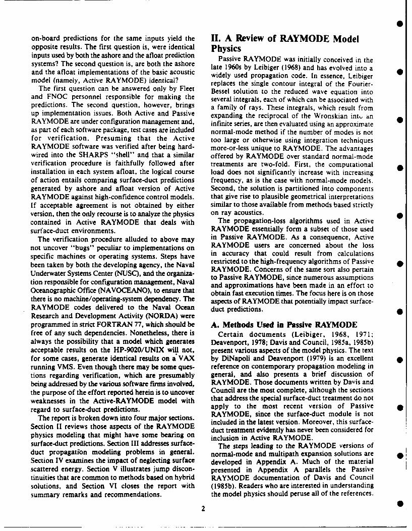
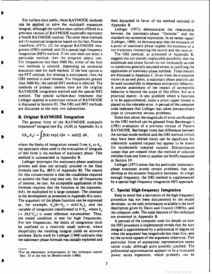
The "mode-leakage" phenomenon is perhaps best where s 3 = P,/#2. The parameters P, and Pl2 areexplained by drawing upon ray analogies. Figure 1 the gradients of the squared index of refractionillustrates a ray trajectory that turns around at the layer for each layer (see Fig. 2). Since I + S 3 = (I + s)depth. To indicate that some of the energy carried by (1 - s + s2), the expression for I RI can be writtenthe ray remains within the duct and that some leaksinto the negative gradient region below, the ray is R = (I - S + s 2) -/(1 + s). (5)split into two components at the turning point.

To extend the ray analogy a bit further, there are T tpartial reflections at th, ray turning points. If U, Thus, the transmission coefficient is given byand K denote, for layer i, two linearly independentsolutions of the depth-separated wave equation, then I TJ = (3s)1'/(l + s). (6)at the layer depth (see Bucker, 1980),

These expressions for JRI and T are in the formsU, + R V = T U2, (2) presented in the RAYMODE documentation of Davis

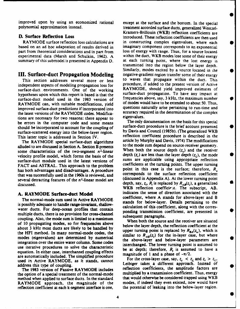
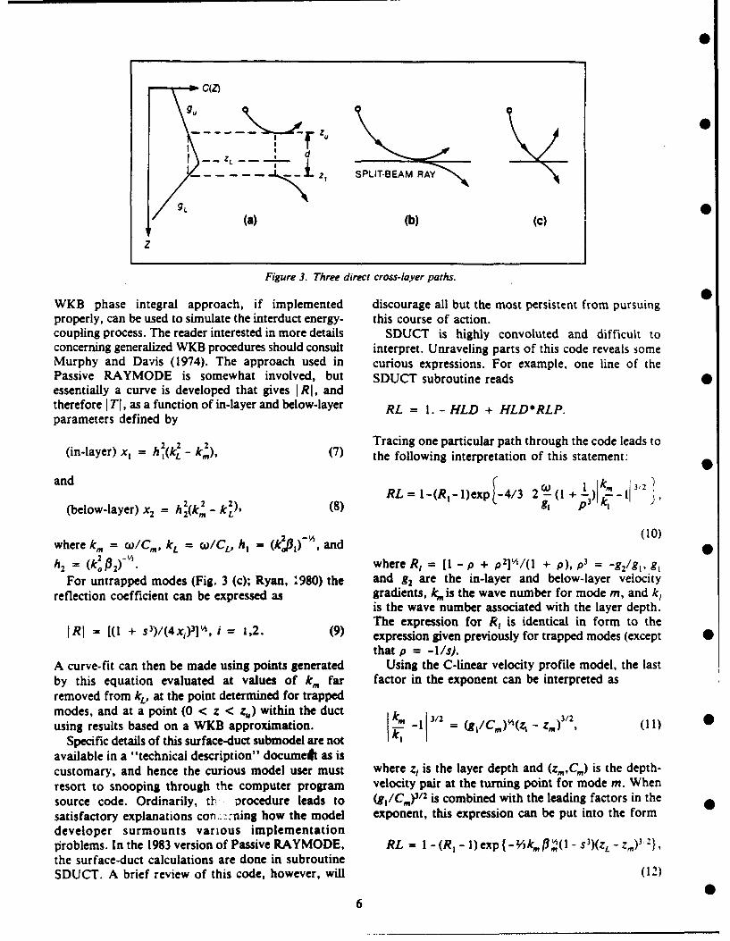
and Council (1985b). Coefficients of the same basicwhere U, and V denote down-going and up-going form can be found in the 1983 RAYMODE computerwaves within the duct (layer 1) and U2 denotes a code, although the definition of s found there isdown-going wave in the region below the duct proportional to the reciprocal of the one defined here.*(layer 2). The reflection and transmission coefficients Figure 3 indicates the ways (excluding surfaceat the bottom of the duct may be obtained from Ryan scattered paths) in which energy can propagate from(1980): an in-layer source to a below-layer receiver. Figure 3

(a) depicts, in terms of ray equivalents, an in-layerJRI 2 = (I + s 3)/(l + S)3 (3) trapped mode and a below-layer untrapped mode.

These modes interact by means of diffraction leakageand through the barrier of thickness'd = z, - z,. Figure 3

(b) illustrates the split-beam ray, corresponding toI T 2 = 1 - JRI

2 , (4) transitional modes, or those modes that are neitherstrongly trapped nor decidedly leaky. Figure 3 (c) showsa steep ray that, in standard ray-acoustical treatments,

C(Z) _ transits directly into the below-layer region.The inclusion of a reflected component is indicative

of the situation associated with a leaky mode. Davis/ ZL and Council (1985v) point out that a generalized

> SPLIT-BEAMS RAY

Z z*This circumstance is a good example of why the physics of

a model, especially one intended for operational applications.Figure 1. Ray trajectory splitting at layer depth- should be fully documented and subjected to peer review.

CO CMZ

C(Z) CO -/31 z n2(Z) 1 3

C(Z) = C0 141 -IlZL + (Z-Z) n2(Z) - 1-Z +0 2 (Z-ZL)

Z zFigure 2. An n2-linear profile for two-layer surface duct (a) sound-velocity profile and (b) index-of-refraction

profile.

5

- C(Z)

S zd

L Z

L 1 SPLI-SEAM RAY

(a) (b) (C)

z

Figure 3. Three direct cross-layer paths.

WKB phase integral approach, if implemented discourage all but the most persistent from pursuingproperly, can be used to simulate the interduct energy- this course of action.coupling process. The reader interested in more details SDUCT is highly convoluted and difficult toconcerning generalized WKB procedures should consult interpret. Unraveling parts of this code reveals someMurphy and Davis (1974). The approach used in curious expressions. For example, one line of thePassive RAYMODE is somewhat involved, but SDUCT subroutine reads 0essentially a curve is developed that gives I R1, andtherefore I TI, as a function of in-layer and below-layer RL = 1. - HLD + HLD*RLP.parameters defined by

2 2 2 Tracing one particular path through the code leads to(in-layer) x, = h 1(kL - kin), (7) the following interpretation of this statement:

andRL = I-(R-l)x -4/3 2 km 3/2RL=)2g(1+-)-1~(below-layer) x2 = h2(k 2 - k2), (8) g, p3 k,

where k. = 0)/Cm, kL = 0)/CL, h, = (k (31) - , and (10)2= (k 2 ) . where R, = [1 - p + p2I'/(l + p), p3 = -g2/g1 , g91

For untrapped modes (Fig. 3 (c); Ryan, :980) the and g2 are the in-layer and below-layer velocityreflection coefficient can be expressed as gradients, k is the wave number for mode m, and k,

is the wave number associated with the layer depth.The expression for R, is identical in form to the

SR1 = [(I + s3)/(4x,)3] ' , i - 1,2. (9) expression given previously for trapped modes (exceptthat p = -1/s).

A curve-fit can then be made using points generated Using the C-linear velocity profile model, the lastby this equation evaluated at values of k. far factor in the exponent can be interpreted asremoved from kL, at the point determined for trappedmodes, and at a point (0 < z < z) within the duct k 13/2 3/2using results based on a WKB approximation. k _- -13 = 4 1,/C.) (z-z.) (11) "

Specific details of this surface-duct submodel are not Iavailable in a "technical description" documeA as iscustomary, and hence the curious model user must where z, is the layer depth and (zmC.) is the depth-resort to snooping through the computer program velocity pair at the turning point for mode m. Whensource code. Ordinarily, th : procedure leads to (g,/C,.) 3 2 is combined with the leading factors in thesatisfactory explanations con -:ning how the model exponent, this expression can be put into the formdeveloper surmounts various implementationproblems. In the 1983 version of Passive RAYMODE, RL = I - (R i - 1) exp { - 2AkI.p3,(l -S 3)(ZL - Z) 2},

the surface-duct calculations are done in subroutineSDUCT. A brief review of this code, however, will (12)

6

where (3,, = 2g 1/C,. The exponent in this last expres- problems. It was adapted for underwater acoustics bysion bears a curious resemblance to exponents typical Marsh (1950) and later refined by Pedersen andof WKB phase-integral functions, except that kft1 'I, Gordon (1965). The Pedersen-Gordon model wasis usually found in place of k,,,' . The dependence subsequently exploited by Watson and McGirr (1966)of this factor on mode number is unexpected and as an integral component of a production-orienteddeserves explanation. performance prediction capability. The primary cus-

Although some of the WKB-type expressions found tomers were local (U.S. Navy Electronic Laboratory-in subroutine SDUCT are similar in basic form to NEL) developers of active sonar systems. At that timethose found in published work (e.g., Barnard computer technology had not advanced to a stageand Deavenport, 1978; Hall, 1976; Kibblewhite and where numerical integration of the z-separated waveDenham, 1965), there are enough differences to equation was considered a viable option. The two-layerwarrant separate documentation. The addition of an normal-mode model, however, offered some promiseupgraded version of SDUCT needs to be considered, as a computationally practicable approach to solvingbecause the inclusion of generalized WKB reflection the surface-duct propagation problem.and transmission coefficients is necessary to obtain The characteristic equation associated with thisrealistic surface-duct predictions using the RAYMODE model takes the form of a 3x3 matrix having elementsnormal-mode sum (but, of course, with more modes). expressible in terms of modified Hankel functions

of order one-third*. These functions were the object ofB. Characteristics of the Bilinear Profile Model intensive investigation by personnel at the Harvard

The special surface-duct treatment reviewed in University Computation Laboratory (1945) duringSection A makes use of the n2-linear velocity profile World War II. Their efforts produced extensive tablesmodel to obtain simple expressions for the generalized valuable for verifying independently developedWKB reflection and transmission coefficients. This computer algorithms, which provide useful informa-profile model has enjoyed wide use in propagation tion regarding power-series and asymptotic-seriescodes, including those based on ray acoustics and representations of the Hankel functions. Thus, withnormal-mode theory. Among normal-mode codes that much of the computational ground work alreadyrely on analytical solutions to the z-separated wave accomplished, incentive to develop a semiautomatedequation for each profile layer, the n2-linear model surface-duct propagation modeling capability was

yields closed-form solutions that can be expressed in strong.terms of Airy functions or modified Hankel functions The Pedersen-Gordon model (also referred to as the

of order one-third. zero-limit profile model; Hall, 1982) requires that two

This profile model also results in straightforward families of modes be considered. The second family

evaluations of range and travel-time integrals, of modes, however, becomes an important considera-

Although the C-linear (constant gradient) profile model tion only at short ranges, at low frequencies, and under

accedes to simple ray-acoustical expressions, it does weak gradient conditions. In this sense, the second

not lend itself quite so readily to wave-acoustical com- family plays a role similar to that of the branch-line

putations. Essentially, the n2-linear profile model integral associated with other branch-cut approaches.

represents a mathematically expedient approach to For most applications, only the first family of modes

solving wave-acoustical problems, and is probably is considered. The procedure adopted at NEL during

satisfactory ior many modeling requirements. Some the late 1960s entailed precalculating first-family eigen-

of the advantages and disadvantages of using models values for selected sets of the controlling parameters.

based on closed-form solutions vice numerical integra- The controlling parameters are p = (gAiga)", where

tion are reviewed in subsection B. I. gA and g. are the above-layer and below-layer

Two features of the n2-linear profile model detract velocity gradients evaluated at the top of each layer,

from its appeal, at least in regard to its appropriateness and M, the so-called "ducting" parameter, defined as

for surface ducts. One feature is the direction ofcurvature, which is sometimes just the opposite of that M = 21'g A'/If "'ZL/C. (13)

suggested by measured profile data; the other is theextreme discontinuity artificially introduced at the layer Thus, for a given value of p, the real and imaginarydepth. This last feature is seldom evident in actual parts of the eigenvalues were calculated and stored forprofiles. The impact of these features is discussed in values of M ranging from I to 100 in steps of 0.25.subsections B.2.-B.4. Needless to say, even for only 60 modes, this procedure

resulted in the storage of thousands of punched cards.1. Computational Pros and Cons

The bilinear normal-mode model was initiallydeveloped by Furry (1945); also see Freehafer, 1951) *In contemporary literature, Airy functions are usually used

to solve tropospheric electromagnetic wave propagation instead.

7

Sets of eigenvalues were calculated and stored for only without problems. The reader interested in furthera few values of p, and predictions had to be limited details on problems that can be encountered is referredto above-layer and below-layer gradients that resulted to Pedersen and McGirr (1982, pp. 97-108).in values of p very close to the few stored values. The Even when a two-layer modeling approach isprocedure for making a prediction entailed selecting applicable, there are some concerns associated with thest. d sets of eigenvalues for values of M on either n2-linear profile model. These concerns are discussedsic..:f that value determined from input data. These in the next few sections.stored sets were then interpolated by the transmissionloss program to arrive at the correct set of eigenvalues. 2. Sharp Discontinuity at the Layer DepthSince the eigenvalues are independent of source-receiver The artificiality of the sharp discontinuity that thegeometry, predictions could be made for several source- a2-linear profile model imposes at the layer dept,, -.asreceiver depth combinations without having to been a source of some concern (Furry, 1946) since therecalculate new sets of eigenvalues. This procedure was model was first exploited. In many instances actualreasonably efficient when predictions were made for velocity profile data exhibit what appears to be a sharpa particular sonar system, i.e., a single frequency. discontinuity. In just as many if not more cases, theWhen predictions had to be made at several frequen- reversal in sign of the gradient is gradual. The conceptcies, the procedure became labor intensive, of layer depth is indeed elusive. Furthermore, even

This approach may seem crude in comparison to when a point can be identified as the layer depth, therecontemporary prediction procedures. Indeed, such is a natural hesitation to proceed with sound fieldmodels as ASTRAL and RAYMODE perform all calculations based on the n2-linear profile mouel.required computations "on the fly," although many Other choices of velocity profile models, completeliberties have been taken by the model developers in with solutions to the reduced wave equation that aremaking approximations to yield relatively fast execu- expressible in terms of well-known tabulated functions,tion times. Kuperman et al. (1986) and Porter et al. are available. For example, the reader is referred to(1987) are developing the Wide-area Rapid Acoustic Murphy and Davis (1974), wherein they discuss the usePrediction (WRAP) system in which certain modal of Weber functions when n2(z) is nearly parabolic.quantities are precalculated at selected spatial nodes The immediate question is, just how many suchin an effort to produce a high-speed three-dimensional possible approaches are needed to address the set ofsound field prediction capability. Thus the idea of all possible profile configurations?precalculating intermediate modal quantities is still There is strong incentive to give serious considera-considered a viable approach in circumventing calcula- tion to propagation models that provide accuratetions that are numerically intensive, solutions for arbitrary velocity profile representations.

There is strong temptation to suggest that a normal- This point is discussed briefly as a recommendationmode model, in conjunction with precalculated sets of in Section V.eigenvalues, be considered for implementation atFNOC to handle the surface-duct propagation predic- 3. Departure from Linearitytion function. The large storage capacity needed to The illustrations in Figure 2 indicate the depth varia-accommodate thousands of precalculated eigenvalues tion in C(Z), as well as in n2(Z). The variation in Cwould not be a serious imposition for shore-based is not quite linear in Z. A question of interest is, whatmainframes. The prol igation modeling commonality impact does this slight departure from linearityrequirement recently issued would necessitate that the (if linearity is indeed the proper criterion) have onsame prediction function be implemented in on-board various intermediate calculations that are involved insystems as well. Computer hardware presently being producing an estimate of the sound field? Since velocityused by on-board systems precludes this possibility, profiles converted from in situ bathythermographsThe addition of an optical disk would lend credence (BTs) do not necessarily exhibit a linear d-pthto a precalculated approach, even for on-board dependence, this question should be asked in referencesystems. to the shape factor associated with a given set of

This approach has considerable appeal from a velocity profile data. As indicated in Appendix F, thestrictly computational point of view. Some disadvan- n2-linear model appears to be a good approximation.tages, however, need to be considered. One of thesedisadvantages pertains to the possible inflexibility of 4. Shape Factora two-layer model. Experimental ,ata (Anderson and The previous discussion indi. !s that the curvaturePedersen, 1976) indicate that other distinct near-surface introduced by the n2-inear pro- : model is negligible.velocity profile configurations are just as prominent Suppose that actual profile data indicate that C3 (Z)as the surface duct. The modeling requirements is linear in depth. Restricting attention to depths downimposed by these other profile configurations to the layer depth, this profile model takes the formdemand a more rigorous multiple-layer treatment.Rigorous solutions are not likely to bemplemented C3(Z) = Co (1 + bZ), (14)

8

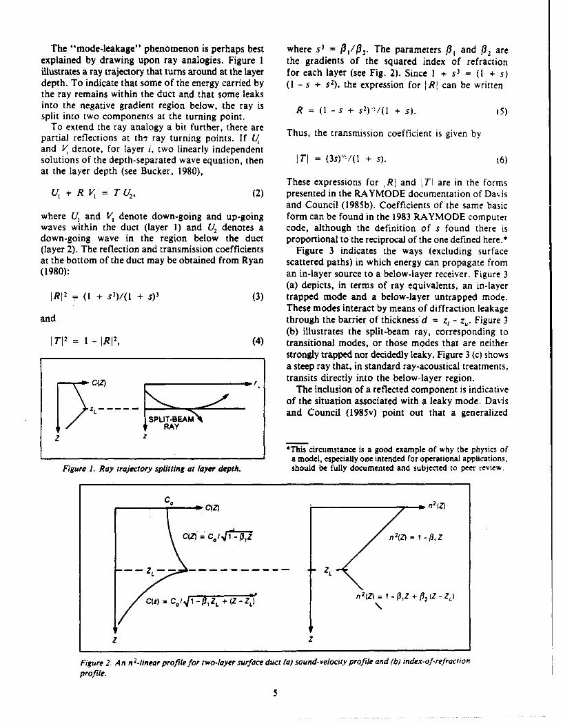
(C0 IC(Z] 2 = 1 -/JZ C3 (Z) = Co(1 + bZ) estimates would be the same. This agreement, alongwith the good agreement between n2-linear andP-C C C3-linear expressions for the modal cycle range

(see Appendix G), suggests that the n2-linear profilen2 -linear C3_1inear model is robust with regard to the shape-factor issue.

zC3 3 dC C IV. Coupling of Surface Scattered EnergyT dz _ - _z _ c9 Z0The primary dissipative contributions to total

Z dZ surface-duct propagation loss are (1) volume absorp-

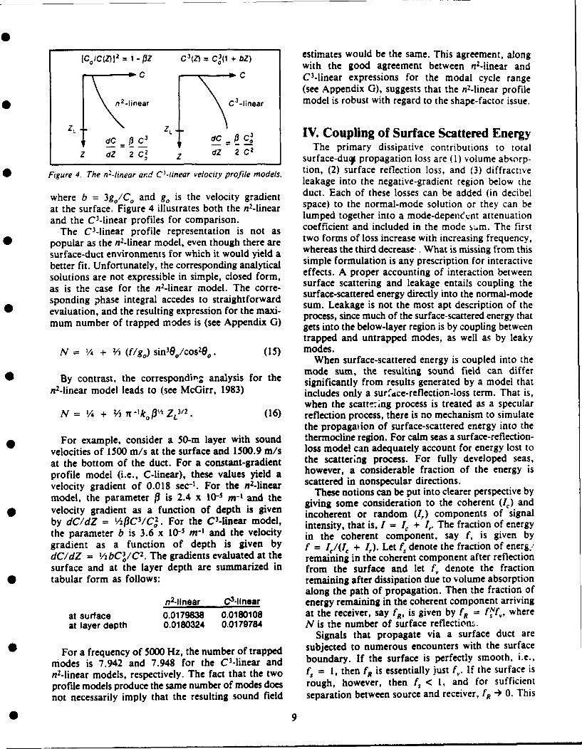
Figure 4. The n -linear and C 3-linear velocity profile models. tion, (2) surface reflection loss, and (3) diffractiveleakage into the negative-gradient region below the

where b = 3go/C o and g, is the velocity gradient duct. Each of these losses can be added (in decibelat the surface. Figure 4 illustrates both the n2-linear space) to the normal-mode solution or they can beand the C3-linear profiles for comparison, lumped together into a mode-depenent attenuation

The C3-linear profile representation is not as coefficient and included in the mode sum. The first

popular as the n2-linear model, even though there are two forms of loss increase with increasing frequency,

surface-duct environments for which it would yield a whereas the third decrease,. What is missing from this

better fit. Unfortunately, the corresponding analytical simple formulation is any prescription for interactivesolutions are not expressible in simple, closed form, effects. A proper accounting of interaction betweenas is the case for the n2-linear model. The torte- surface scattering and leakage entails coupling the

sponding phase integral accedes to straightforward surface-scattered energy directly into the normal-modeevaluation, and the resulting expression for the maxi- sum. Leakage is not the most apt description of themvauanumberao tred mesulting ex i n e n i ) process, since much of the surface-scattered energy thatmum number of trapped modes is (see Appendix G) gets into the below-layer region is by coupling between

trapped and untrapped modes, as well as by leakyN = / + 13 (flg0 ) sin3Oo/cOs 2

0 . • (15) modes.When surface-scattered energy is coupled into the

By contrast, the corresponding analysis for the mode sum, the resulting sound field can differa i significantly from results generated by a model that

n2-linear model leads to (see McGirr, 1983) includes only a surface-reflection-loss term. That is,when the scatte-ing process is treated as a specular

N = '/ + 3 71 'kofl13 ZL312 . (16) reflection process, there is no mechanism to simulatethe propagaiion of surface-scattered energy into the

For example, consider a 50-m layer with sound thermocline region. For calm seas a surface-reflection-velocities of 1500 m/s at the surface and 1500.9 m/s loss model can adequately account for energy lost toat the bottom of the duct. For a constant-gradient the scattering process. For fully developed seas,profile model (i.e., C-linear), these values yield a however, a considerable fraction of the energy is

velocity gradient of 0.018 sec-1. For the n2-linear scattered in nonspecular directions.model, the parameter /3 is 2.4 x 10- -in-' and the These notions can be put into clearer perspective bymoelcthe araeter s 2.4 xunctionofadep thge giving some consideration to the coherent (4c) andvelocity gradient as a function of depth is given incoherent or random (,) components of signalby dC/dZ = zrm3C . For the C-linear model, intensity, that is, I = 1, + 4. The fraction of energythe parameter b is 3.6 x 10-i mi and the velocity in the coherent component, say f, is given bygradient as a function of depth is given by f = 4/(I + I,). Let f, denote the fraction of energ:dC/dZ = bCo/C 2 . The gradients evaluated at the remaining in the coherent component after reflectionsurface and at the layer depth are summarized in from the surface and let f, denote the fractiontabular form as follows: remaining after dissipation due to volume absorption

along the path of propagation. Then the fraction ofn2-lnear C3-11near energy remaining in the coherent component arriving

at surface 0.0179838 0.0180108 at the receiver, say f,, is given by tn = f~f, whereat layer depth 0.0180324 0.0179784 N is the number of surface reflections.

Signals that propagate via a surface duct are

For a frequency of 5000 Hz, the number of trapped subjected to numerous encounters with the surface

modes is 7.942 and 7.948 for the C3-linear and boundary. If the surface is perfectly smooth, i.e.,

n2-linear models, respectively. The fact that the two f, = 1, then fR is essentially just f,. If the surface is

profile models produce the same number of modes does rough, however, then f, < 1, and for sufficientnot necessarily imply that the resulting sound field separation between source and receiver, fR -4 0. This

*- 9

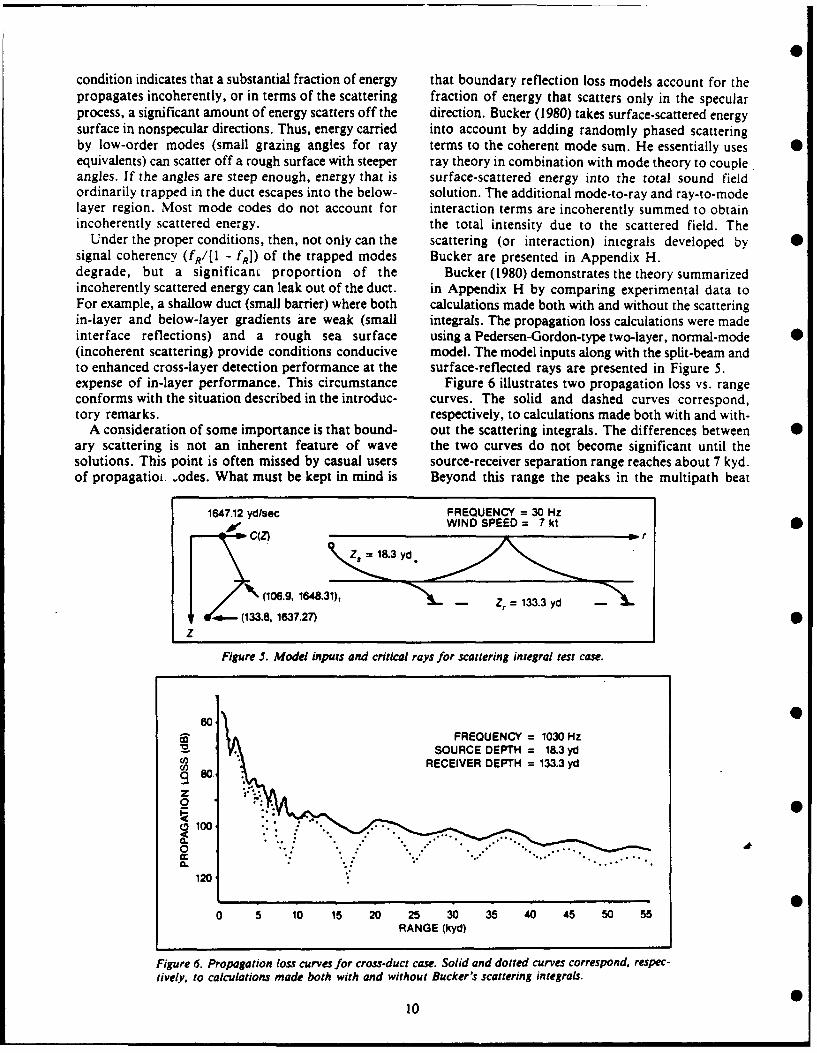
condition indicates that a substantial fraction of energy that boundary reflection loss models account for thepropagates incoherently, or in terms of the scattering fraction of energy that scatters only in the specularprocess, a significant amount of energy scatters off the direction. Bucker (1980) takes surface-scattered energysurface in nonspecular directions. Thus, energy carried into account by adding randomly phased scatteringby low-order modes (small grazing angles for ray terms to the coherent mode sum. He essentially uses 0equivalents) can scatter off a rough surface with steeper ray theory in combination with mode theory to coupleangles. If the angles are steep enough, energy that is surface-scattered energy into the total sound fieldordinarily trapped in the duct escapes into the below- solution. The additional mode-to-ray and ray-to-modelayer region. Most mode codes do not account for interaction terms are incoherently summed to obtainincoherently scattered energy. the total intensity due to the scattered field. The

Under the proper conditions, then, not only can the scattering (or interaction) integrals developed by Ssignal coherency (fR/[I - fR]) of the trapped modes Bucker are presented in Appendix H.degrade, but a significant proportion of the Bucker (1980) demonstrates the theory summarizedincoherently scattered energy can leak out of the duct. in Appendix H by comparing experimental data toFor example, a shallow duct (small barrier) where both calculations made both with and without the scatteringin-layer and below-layer gradients are weak (small integrals. The propagation loss calculations were madeinterface reflections) and a rough sea surface using a Pedersen-Gordon-type two-layer, normal-mode 0(incoherent scattering) provide conditions conducive model. The model inputs along with the split-beam andto enhanced cross-layer detection performance at the surface-reflected rays are presented in Figure 5.expense of in-layer performance. This circumstance Figure 6 illustrates two propagation loss vs. rangeconforms with the situation described in the introduc- curves. The solid and dashed curves correspond,tory remarks. respectively, to calculations made both with and with-

A consideration of some importance is that bound- out the scattering integrals. The differences between 0ary scattering is not an inherent feature of wave the two curves do not become significant until thesolutions. This point is often missed by casual users source-receiver separation range reaches about 7 kyd.of propagatioi. odes. What must be kept in mind is Beyond this range the peaks in the multipath beat

1647.12 yd/sec FREQUENCY = 30 HzWIND SPEED=7 t r

Z =1 8.3yd

648.31), - Zr = 133.3yd

(133.8, 1637.27)z

Figure S. Model inputs and critical rays for scattering integral test case.

600FREQUENCY = 1030 Hz

SOURCE DEPTH = 18.3 ydRECEIVER DEPTH = 133.3 yd

9 s

120

RANGE (kyd)

Figure 6. Propagation Ios$s curves for cross-duct case. Solid and dotted curves correspond, respec-tively, to calculations made both with and without Bucker's scattering integrals.

10

structure are 1-2 dB more optimistic for the solid curve. SOURCE DEPTH = 6 mThe interference nulls for this curve are noticeably less RECEIVER DEPTH = 18 mextreme. This latter feature is a characteristic directly FREQUENCY = 2300 Hzattributable to the contribution of incoherently scat- WIND SPEED = 0 kttered energy.

Similar comparisons for the in-layer case are not c(Z)available, although Bucker (1980) notes that the differ- DUCT #1ences are not as dramatic for this case. He further notes DU0 Mthat the major differences occur in the interference- --- 00mnulls where incoherently scattered energy tends to fillin the sound field. ? 1526.8 mis

The interpretation of these results with regard to the DUCT #2main issue-anomalous SHARPS-generated surface-duct predictions-is that even though calculationsbased on the scattering integrals yield more realistic --- -- 1000 m

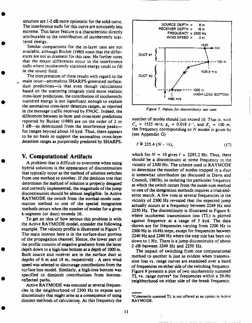
[ (HIGH-LOSS BOTTOM)cross-layer predictions, the contribution of incoherently Z140 mH Oscattered energy is not significant enough to explainthe anomalous cross-layer detection ranges, as reportedin the message traffic received by FNOC. Indeed, the Figure 7. Inputs for discontinuity test case.differences between in-layer and cross-layer predictions number of modes should just exceed 10. That is, withreported by Bucker (1980) are on the order of 2 or C = 1525 ms, g, = 0.018 s-I, and Z = 100 M,3 dB-as determined from the interference peaks- the frequency corresponding to N modes is given byfor ranges beyond about 10 kyd. Thus, there appears theefAppency G)

to be no basis to support the anomalous cross-layer (see Appendix G)detection ranges as purportedly predicted by SHARPS. f235.4 (N- ), (17)

V. Computational Artifacts which for N = 10 gives f = 2295.2 Hz. Thus, thereshould be a discontinuity at some frequency in the

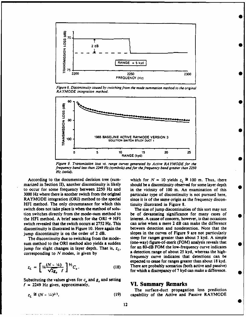
A problem that is difficult to overcome when using vicinity of 2300 Hz. The scheme used in RAYMODEhybrid solutions is the appearance of discontinuities to determine the number of modes trapped in a ductthat typically occur as the method of solution switches is somewhat unorthodox (as discussed in Davis andfrom one method to another. If the decision tree that Council, 1985b), so isolating the particular frequencydetermines the method of solution is properly designed at which the switch occurs from the mode-sum methodand correctly implemented, the magnitude of the jump to one of the integration methods requires a trial-and-discontinuities should be almost negligible. In Active error search. A few runs at several frequencies in theRAYMODE the switch from the normal-mode sum- vicinity of 2300 Hz revealed that the expected jumpmation method to one of the special integration actually occurs at a frequency between 2249 Hz andmethods occurs when the number of modes for a given 2250 Hz. The discontinuity is illustrated in Figure 8,k-segment (or duct) exceeds 10. where incoherent transmission loss (TL) is plotted

To get an idea of how serious this problem is with against frequency at a range of 5 kyd. The datathe Active RAYMODE model, consider the following shown are for frequencies varying from 2200 Hz toexample. The velocity profile is illustrated in Figure 7. 2300 Hz in 10-Hz steps, except for frequencies betweenThe main interest here is in the surface-duct portion 2240 Hz and 2260 Hz where the step size has been cutof the propagation channel. Hence, the lower part of down to 1 Hz. There is a jump discontinuity of aboutthe profile consists of negative gradients from the layer 2 dB between 2249 Hz and 2250 Hz.depth down to a high-loss bottom at a depth of 1000 m. The impact of switching from one computationalBoth source and receiver are in the surface duct at method to another is just as evident when transmis-depths of 6 m and 18 m, respectively A zero wind sion loss vs. range curves are examined over a bandspeed was selected to discourage contributions from the of frequencies on either side of the switching frequency.surface loss model. Similarly, a high-loss bottom was Figure 9 presents a plot of two incoherently summedspecified to diminish contributions from bottom- TL vs. range curves* for frequencies within a 50-Hzreflected paths. neighborhood on either side of the break frequency.

Active RAYMODE was executed at several frequen-cies in the neighborhood of 2300 Hz to expose anydiscontinuity that might arise as a consequence of using *Coherently summed TL is not offered as an option in Activedistinct methods of calculation. At this frequency the RAYMODE.

1

70.

o~ 2dBz

0

zx 75ky1

2200 2250 2300FREQUENCY (Hz)

Figure 8. Discontinuity caused by switching from the mode summation method to the originalRA YMODE integration method.

60

z 8 0 .074

t occu 1985 BASELINE ACTiVE RAYMODE VERSION 3

0 5 10 15 20 25RANGE (kyd)

Figure . Transmission loss vs. range curves generated by Active RA YMODE for thefrequency band less than 2249 Hz (symbols) and for the frequency band greater than 2250Hz (solid).

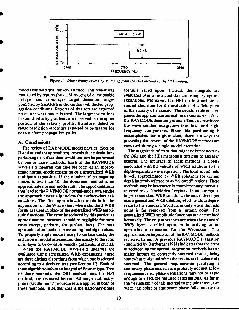
According to the documented decision tree (sum- which for N = 10 yields ZL 2 100 m. Thus, theremarized in Section 11), another discontinuity is likely should be a discontinuity observed for some layer depthto occur for some frequency between 2250 Hz and in the vicinity of 100 m. An examination of this3000 Hz where there is another switch from the original particular type of discontinuity is not pursued here,RAYMODE integration (ORI) method to the special since it is of the same origin as the frequency discon-HF method. The only circumstance for which this tinuity illustrated in Figure 8.switch does not take place is when the method of solu- The size of jump discontinuities of this sort may nottion switches directly from the mode-sum method to be of devastating significance for many cases ofthe HFO method. A brief search for the ORa s) HE interest. A cause of concern, however, is that occasionsswitch revealed that the switch occurs at 2752 Hz. This can arise when a mere 2 dB can make the differencediscontinuity is ustrated in Figure 10. Here again the between detection and nondetection. Note that thejump discontinuity is on the order of 2 dB. slopes in the curves of Figure 9 are not particularly

The discontinuity due to switching from the mode- steep for ranges greater than about 5 kyd. A simplesum method to the ORI method also yields a sudden (one-way) figure-of-merit (FOM) analysis reveals thatjump for slight changes in layer depth. That is, , for an 80-dB FOM the low-frequency curve indicatescorresponding to N modes, is given by a detection range of about 25 kyd, whereas the high-

frequency curve indicates that detections can be

ZL =~ N A [3 expected to cease for ranges greater than about 18 kyd.4( V - /4 . -(18) There are probably scenarios (both active and passive)

2g, for which a discrepancy of 7 kyd can make a difference.

Substituting the values given for c. and g. and settingf = 2249 Hz gives, approximately, V1. Summary Remarks

The surface-duct propagation loss predictionZL gl (N- )z' 3, (19) capability of the Active and Passive RAYMODE

12

I-70

,RANGE -5 kyd0

z

0

75

- 2700 2750 2800FREQUENCY (Hz)

Figure 10. Discontinuity caused by switching from the ORI method to the HF! method.

models has been qualitatively assessed; This review was formula relied upon. Instead, the integrals aremotivated by reports (Naval Messages) of questionable evaluated over a restricted domain using asymptoticin-layer and cross-layer target detection ranges expansions. Moreover, the HFI method includes apredicted by SHARPS under certain well-ducted prop- special algorithm for the evaluation of a field pointagation conditions. Reports of this sort are expected in the vicinity of a caustic. The decision rule encom-no matter what model is used. The largest variations passes the approximate normal-mode sum as well; thus,in sound-velocity gradients are observed in the upper the RAYMODE decision process effectively partitionsportion of the velocity profile; therefore, detection the wave-number integration into low- and high-range prediction errors are expected to be greater for frequency components. Since this partitioning isnear-surface propagation paths. accomplished for a given duct, there is always the

A. Conclusions possibility that several of the RAYMODE methods are

The review of RAYMODE model physics, (Section exercised during a single model execution.

II and attendant appendices), reveals that calculations The magnitude of error that might be introduced by

pertaining to surface-duct conditions can be performed the ORI and the HFI methods is difficult to assess in

by one or more methods. Each of the RAYMODE general. The accuracy of these methods is closelywave-field integrals can take the form of an approx- associated with the validity of WKB solutions to the

imate normal-mode expansion or a generalized WKB depth-separated wave equation. The local sound fieldmultipath expansion. If the number of propagating is well approximated by WKB solutions for certainmodes is less than 10, the dominant method is an depth intervals referred to as "allowed" regions. Theseapproximate normal-mode sum. The approximations methods may be inaccurate in complementary intervals,that lead to the RAYMODE normal-mode sum render referred to as "forbidden" regions. In an attempt tothe approach essentially useless for surface-duct cal- improve standard WKB solutions, the model developerculations. The first approximation made is in the uses a generalized WKB solution, which tends to degen-expression for the Wronskian, where standard W KB crate to the standard W KB form only when the fieldforms are used in place of the generalized WKB ampli- point is far removed from a turning point. Thetude functions. The error introduced by this particular generalized WKB amplitude functions are determinedapproximation, however, should be negligible for most iteratively. The only other instance when the standardcases except, perhaps, for surface ducts. The next WKB form is relied upon, is in arriving at anapproximation made is in assuming real eigenvalues. approximate expression for the Wronskian. ThisTo properly apply mode theory to surface ducts, the approximation impacts all of the RAYMODE methodsinclusion of modal attenuation, due mainly to the ratio reviewed herein. A previous RAYMODE evaluationof in-layer to below-layer velocity gradients, is crucial. conducted by Bartberger (1981) indicates that the error

When the RAYMODE wave-field integrals are introduced by the special integration methods has itsevaluated using generalized WKB expansions, there major impact on coherently summed results, beingare three distinct algorithms from which one is selected somewhat mitigated when the results are incoherentlyaccording to a decision tree (see Section II). Each of summed. The general requirements justifying athese algorithms solves an integral of Fourier type. Two stationary-phase analysis are probably not met at lowof these methods, the ORI method, and the HFI frequencies, i.e., phase oscillations may not be rapidmethod, are reviewed herein. Although stationary- enough to effect the required cancellations. As far asphase (saddle-point) procedures are applied in both of the "extension" of this method to include those casesthese methods, in neither case is the stationary-phase when the point of stationary phase falls outside the

13

limits of integration is concerned, the procedure used (reduce the loss) by 2 dB for the longer ranges. Justin RAYMODE appears to have been chosen out of as importantly, the interference nulls tend to get washedconvenience, i.e., so that the Fresnel integral algorithms out. For detection range calculations based on coherentcan be used. The specific steps taken by the model signal-to-noise ratios, the contribution of incoherentlydeveloper in applying stationary-phase methods are s.attered energy would be significant, but only if the 0not universally accepted as being the most effective correct statistical distributions are considered (as(see Weinberg, 1981). discussed in Pedersen and McGirr, 1983). If only

The surface reflection loss submodel is reviewed in averaged signal-to-noise ratios are considered, theSection I. An estimate of surface loss (SL) is deter- significance is less dramatic. Considerationmined from the sum of two independent terms, SL, should be given to including the scattering integrals,and SL 2 . The evaluation by Keenan (1983) of the since their omission can yield slightly pessimistic cross- 0SUBCOM surface loss model (the one used in layer predictions.RAYMODE) shows that the SL, term represents Discontinuities that occur when the method of solu-incoherently scattered energy characteristic of a tion switches from one form to another appear to beKirchhoff solution. Keenan further notes that this term on the order of a couple of decibels, at least as deter-is dominant for frequencies below about 1 kHz. Since mined by the brief assessment presented herein.incoherent scattering should dominate the solution only Numerical artifacts of this sort fall into the category 0for large values of the Rayleigh parameter, Keenan of nuisances and are typical of hybrid methods. Toconcludes that the SL, term is not intuitively satisfac- the extent that the size of these discontinuities does nottory as an estimator of rough surface loss. exceed about 2 dB, they are not considered to be major

The SL 2 term has no angle dependence, and it is deficiencies.probably supposed to represent the coherent compo- In any case, none of the Active RAYMODE modelnent of energy scattered at an average angle deficiencies discussed herein is likely to causecharacteristic of surface-duct and convergence zone anomalous cross-layer detection ranges, such as thosepaths. Speculation of this sort is interesting, although purportedly predicted by SHARPS. The verynot particularly productive. Until the model developer appearance of anomalous surface-duct detection rangessubjects his derivation to peer review, however, any generated by SHARPS naturally raises the question,critique of the model physics amounts to little more what set of surface-duct conditions could possiblythan speculation. Results generated by this model were produce greater detection ranges for cross-layer •evaluated, along with results generated by several other geometries than for in-layer geometries? For a well-surface loss models. Comparisons are included in a defined classic surface duct, an answer is notreport that presents the findings and recommendations immediately forthcoming. If care is not taken inof a surface loss model working group (Eller, 1984). identifying-acoustically-what does or does notInterestingly, the surface loss model recommended by constitute a well-defined surface duct, then interpreta-this working group has not been adopted. tions of the resulting acoustic predictions are

A special surface-duct leakage routine, included in more-or-less at the mercy of possibly invalid interpreta-a previous version of Passive RAYMODE, is con- tions of the controlling velocity profile. This latterspicuously missing from the present version. A review possibility essentially reflects the essence of theof the corresponding computer code reveals at least so-called sonic-layer-depth (SLD) problem.one error, along with expressions that bear a curious As a case in point, consider the following example.resemblance to those normally associated with WKB Suppose the input velocity profile (as generated by aphase integral methods. Corrections could be made pre-SHARPS program) takes the form illustrated inquite readily, although suggestions offering more Figure 11. The near-surface portion of this profilepromise are made in the recommendations section. consists of an isovelocity duct overlaying a weak

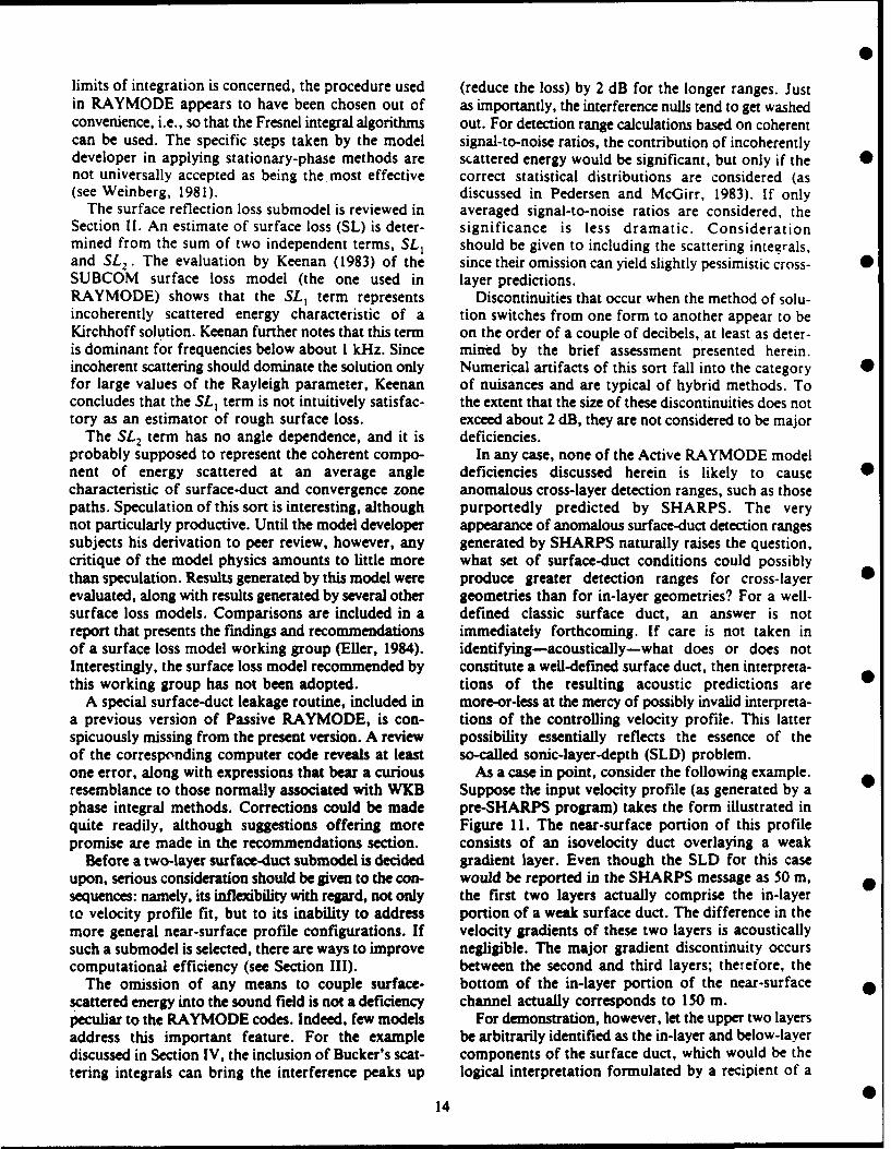
Before a two-layer surface-duct submodel is decided gradient layer. Even though the SLD for this caseupon, serious consideration should be given to the con- would be reported in the SHARPS message as 50 m,sequences: namely, its inflexibility with regard, not only the first two layers actually comprise the in-layerto velocity profile fit, but to its inability to address portion of a weak surface duct. The difference in themore general near-surface profile configurations. If velocity gradients of these two layers is acousticallysuch a submodel is selected, there are ways to improve negligible. The major gradient discontinuity occurscomputational efficiency (see Section III). between the second and third layers; therefore, the

The omission of any means to couple surface- bottom of the in-layer portion of the near-surfacescattered energy into the sound field is not a deficiency channel actually corresponds to 150 m.peculiar to the RAYMODE codes. Indeed, few models For demonstration, however, let the upper two layersaddress this important feature. For the example be arbitrarily identified as the in-layer and below-layerdiscussed in Section IV, the inclusion of Bucker's scat- components of the surface duct, which would be thetering integrals can bring the interference peaks up logical interpretation formulated by a recipient of a

14

SONAR DEPTH = 6 in 1985 BASELINE ACTIVE RAYMOOE VERSION 3TARGET DEPTH = 18 m/100 m

FREQUENCY = 3000 Hz 60

WIND SPEED = 0 kt

1535 m s

LAYER 1 )0 (a) "IN-LAYER"Cn 80-

a-- 50 m n (b) "CROSS-LAYER"

LAYER 2 z 90 -0

- - - - 150 m S2100 ,_ 1534.9 0 4

z 110.(b)

120(a)

1000m 130z (HIGH-LOSS BOTTOM) 0 10 20 30 40 50

1480 m/s RANGE (kyd)

Figure I. Sound velocity profile for an SLD test case. Figure 12. Transmission loss curves for an SLD test case.

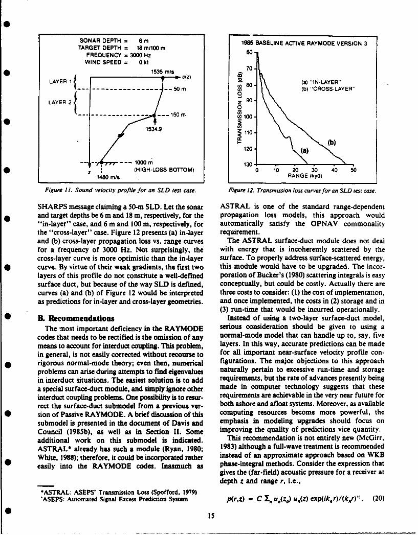
SHARPS message claiming a 50-m SLD. Let the sonar ASTRAL is one of the standard range-dependentand target depths be 6 m and 18 m, respectively, for the propagation loss models, this approach would"in-layer" case, and 6 m and 100 m, respectively, for automatically satisfy the OPNAV commonalitythe "cross-layer" case. Figure 12 presents (a) in-layer requirement.and (b) cross-layer propagation loss vs. range curves The ASTRAL surface-duct module does not dealfor a frequency of 3000 Hz. Not surprisingly, the with energy that is incoherently scattered by thecross-layer curve is more optimistic than the in-layer surface. To properly address surface-scattered energy,curve. By virtue of their weak gradients, the first two this module would have to be upgraded. The incor-layers of this profile do not constitute a well-defined poration of Bucker's (1980) scattering integrals is easysurface duct, but because of the way SLD is defined, conceptually, but could be costly. Actually there arecurves (a) and (b) of Figure 12 would be interpreted three costs to consider: (1) the cost of implementation,as predictions for in-layer and cross-layer geometries. and once implemented, the costs in (2) storage and in

(3) run-time that would be incurred operationally.B. Recommendations Instead of using a two-layer surface-duct model,

The most important deficiency in the RAYMODE serious consideration should be given to using acodes that needs to be rectified is the omission of any normal-mode model that can handle up to, say, fivemeans to account for interduct coupling. This problem, layers. In this way, accurate predictions can be madein general, is not easily corrected without recourse to for all important near-surface velocity profile con-rigorous normal-mode theory; even then, numerical figurations. The major objections to this approachproblems can arise during attempts to find eigenvalues naturally pertain to excessive run-time and storagein interduct situations. The easiest solution is to add requirements, but the rate of advances presently beinga special surface-duct module, and simply ignore other made in computer technology suggests that theseinterduct coupling problems. One possibility is to resur- requirements are achievable in the very near future forrect the surface-duct submodel from a previous ver- both ashore and afloat systems. Moreover, as availablesion of Passive RAYMODE. A brief discussion of this computing resources become more powerful, thesubmodel is presented in the document of Davis and emphasis in modeling upgrades should focus on

Council (1985b), as well as in Section II. Some improving the quality of predictions vice quantity.

additional work on this submodel is indicated. This recommendation is not entirely new (McGirr,ASTRAL already has such a module (Ryan, 1980; 1983) although a full-wave treatment is recommendedWhite, 1988); therefore, it could be incorporated rather instead of an approximate approach based on WKB

easily into the RAYMODE codes. Inasmuch as phase-integral methods. Consider the expression thatgives the (far-field) acoustic pressure for a receiver atdepth z and range r, i.e.,

*ASTRAL: ASEPS' Transmission Loss (Spofford. 1979)'ASEPS: Automated Signal Excess Prediction System p(r,z) = C I'R u.(z,) u.(z) exp(iknr)/(k,,r)'1, (20)

15

where z. is the source depth, and the u. are normal- is also d~cussed by McGirr (1983) and by Renner andized modal depth functions. The k, (eigenvalues) are Kirby (1983). Since the anomalous SHARPS predic-functions of frequency and the environmental-acoustic tions are in contrast with those generated by shipboardinput profile (velocity profile, bottom depth, bottom prediction systems, (the latter results are purportedlyloss, and surface loss), but they are independent of the more reasonable) the OPNAV imposed com- *source depth and receiver depth. The u,,(z) are func- monality requirement needs to be extended to includetions of the k,. Thus, there is a natural hierarchical any and all peripheral software and data bases thatordering of the required computations for any given can impact predictions generated by standard acousticrun. models. Thus, as a final recommendation, the organi-

Suppose that predictions are required for a single zation responsible for configuration control of Fleetsource depth and three receiver depths at some acoustic prediction systems should ensure that ali uch *frequency, say, fo, for which there are N modes. First software packages and data bases essentially producethe N eigenvalues are determined and stored. Then, identical results. For the case at hand, this action entailsthe depth functions {u,,(z 0)} are computed and replacing the BT-conversion software presently usedstored. Then, three sets of N depth functions {u,,(z)}, at FNOC with the appropriate software that isj = 1, 2 and 3, are computed and stored. For each used by (standard) shipboard prediction systems.receiver depth (z), a transmission loss vs. range curve 0can be determined from

VII. ReferencesTL -10 log Ipp . (21) Anderson, E. R. and M. A. Pedersen (1976).

Surface-Duct Sonar Measurements (SUDS I - 1972).where, for long ranges, the normalized acoustic Technical Report, Naval Undersea Center, San Diego,pressure is given by CA, NUC TP 463.

Barnard, G. R. and Deavenport, R. L. (1978).p = I. A,, u,(z) exp(ikr)/Vr, (22) Propagation of sound in underwater surface chan-

nels with rough boundaries. J. Acoust. Soc. Am.and where A,, = C u,(zo)/ kn. The expression for p 63:709-714.has been put into this form to emphasize that the A. Bartberger, C. L. (1981). An Investigation of theare simply retrieved from storage during this stage of Physics of the RA YMODE Model. Naval Air Develop-computation. The number of terms in the sum is ment Center, Warminster, PA, NADC Reportactually a function of range. That is, modal attenua- 82009-30.tion increases with range, therefore, fewer terms are Beckmann, P. and A. Spizzichino (1963). The Scat-needed as range increases. A relatively conservative tering of Electromagnetic Waves from Rough Surfaces.criterion used in determining when to stop the sum- Macmillan, New York.mation entails comparing the last four terms to the Bleistein, N. and R. A. Handelsman (1986). Asymp-cumulative sum. If the relative contribution is less than totic Expansions of Integrals. Dover, New York.0.0001, then the summation is stopped. Brekhovskikh, L. M. (1980). Waves in Layered

The computational strategy described above can be Media. Academic Press, Inc., New York, 2nd edition.exploited even more aggressively in the design of Brekhovskikh, L. M. and Yu. Lysanov (1982).prediction systems dedicated to the generation of data Fundamentals of Ocean Acoustics. Springer-Verlag, 0in support of predeployment acoustic assessments. New York.Assessments of this sort are typically based on archived Bucker, H. P. (1970). Sound propagation in a chan-data. Standard Navy data bases could be expanded to nel with lossy boundaries. J. Acoust. Soc. Am.include precalculated intermediate modal quantities 48:1187-1194.tailored to specific system parameters and most- Bucker, H. P. (1980). Wave propagation in a ductprobable target depths. This procedure is similar to with boundary scattering (with application to a sur-the one discussed in Section II. To incorporate updated face duct). J. Acoust. Soc. Am. 68:1768-1772.oceanographic data, however, would require adding Cox, C. S. and W. H. Munk (1954). Measurementa perturbation scheme, or, using a prediction system of the roughness of the sea surface from photographssuch as WRAP, which is presently under development of the sun glitter. J. Optic. Soc. Am. 44:838-850.by Kuperman et al. (1986) and Porter et al. (1987). Davis, J. A. and 0. P. Council (1985a). ACTIVE

Finally, insofar as anomalous SHARPS-generated, RA YMODE. Planning Systems Inc., McLean, VA.cross-layer detection ranges are concerned, this cir- PSI TR-$310045.cumstance is more than likely a consequence of the Davis, J. A. and 0. P. Council (1985b). PASSIVElong-standing SLD problem, as mentioned in the intro- RA YMODE. Planning Systems Inc., McLean, VA,duction and discussed in the conclusions. This problem PSI TR-S310046.

16

Deavenport, R. L. (1978). RA YMODE Physics Leibiger, G. A. (1968). Application of Normal ModeEvaluation. Naval Undersea Systems Center, New Theory to Propagation of 3.5 kHz Pulses in ShallowLondon, CT, Encl(2) to NUSC/NL ltr ser 9312-55. Water. Vitro Laboratories, VL-2476-9-O.

DiNapoli, F. R. and Deavenport, R. L. (1979). Leibiger, G. A. (1971). A Combined Ray Theory-Numerical Models of Underwater Acoustic Propaga- Normal Mode Approach to Long Range, Lowtion. In Ocean Acoustics, Chap. 3, by J. A. DeSanto Frequency Propagation Loss Prediction. Naval Under-(ed.), Springer-Verlag, New York. water Sound Center, New London, CT, NUSC

Eller, A. (1984). Findings and Recommendations of Technical Memorandum PA3-0109-71.the Surface Loss Model Working Group: Final Report.Naval Ocean Research and Development Activity, Marsh, H. W. (1950). Theory of Anomalous Pro-Stennis Space Center, MS, NORDA TN 279. pagation of Acoustic Waves in the Ocean. U.3.N.

Erdlyi, A. (1956). Asymptotic Expansions. Dover, Underwater Sound Laboratory, New London, CT,New York. USNUSL Report I11.

Freehafer, J. E. (1951). Phase-integral Methods, and Marsh, H. W. and M. Schulkin (1962). UnderwaterThe Field Integral, (Sect 2.10). In Propagation of Short Sound Transmission. AVCO Marine Electronics OfficeRadio Waves, D.E. Kerr (ed.), McGraw-Hill, New (unpublished technical memorandum).York, sect. 2.8 and 2.10. McGirr, R. W. (1983). Comments and Issues Perti-

Furry, W. H. (1945). Methods of Calculating nent to SHARPS III Near-surface PropagationCharacteristic Values for Bilinear M Curves. Modeling. Naval Ocean Research and DevelopmentMassachusetts Institute of Technology, Boston, MA, Activity, Stennis Space Center, MS, NORDAMIT Laboratory Report 680. Report 64.

Furry, W. H. (1946). Theory of Characteristic Func- McGirr, R. W., L. K. Arndt and E. D. Chaikations in Problems of Anomalous Propagation. (1972). Fast NISSM, A Utility Version of the NavyMassachusetts Institute of Technology, Boston, MA, Interim Surface Ship Sonar Prediction Model. NavalMIT Laboratory Report 795. Undersea Research and Development Center, San

Gordon, D. F. and H. P. Bucker (1984). Arctic Diego, CA, NUC TP-309.Acoustic Propagation Model with Ice Scattering, Naval Murphy, E. . nd J. A. Davis (1974). Modified rayOcean Systems Center, San Diego, CA, NOSC TR 985.

Hall, M. (1976). Mode theory of wave propagation theory for bounded media. J. Acoust. Soc. Am. 56:in a bilinear medium: The WKB approximation. 1747-1760.J. Acoust. Soc. Am. 60:810-814. Pedersen, M. A. and D. F. Gordon (1965). Normal

Hall, M. (1982). Normal mode theory: The role of mode theory applied to short-range propagation in anthe branch-line integral in Pedersen-Gordon type underwater acoustic surface duct. J. Acoust. Soc. Am.models. J. Acoust. Soc. Am. 72:1978-1988. 37:105-118.

Harvard University Computation Laboratory (1945). Pedersen, M. A. and R. W. McGirr (1982). Use ofTables of the Modified Hankel Functions of Order Theoretical Controls in Underwater Acoustic ModelOne-Third and of Their Derivatives, Vol. I1. Harvard Evaluation. Naval Ocean Systems Center, San Diego,University Press, Cambridge, MA. CA, NOSC TR 758.

Houston, R. A. (1915). A Treatise on Light. Pedersen, M. A. and R. W. McGirr (1983).Longmans, Green & Co., New York. Experimental and Theoretical Statistical Distributions

Keenan, R. E. (1983). Final Report Volume IV.- of Underwater Acoustic Propagation Losses. PresentedSUECOM, FAME, RA YMODE and FACT Corn- at the 1 th International Congress of Acoustics, Paris,parisons of Accuracy and Computation Time in a Paper 28-11Surface Duct Environment. Science Applications Inc., Pper 28-11McLean, VA, SAI-84-153-WA. Porter, M. B., W. A. Kuperman, F. Ingenitoand

Kibblewhite, A. C. and R. N. Denham (1965). A.A. Piacsek (1987). Rapid computation of acousticExperiment on propagation in a surface sound chan- fields in three-dimensional ocean environments.nel. J. Acoust. Soc. Am. 38:63-71. J. Acoust. Soc. Am. 81(SI):$9.

Kirby, W. D. (1982). Technical Description for the Renner, W. W. and W. D. Kirby (1983). SoundShip Helicopter Acoustic Range Prediction System Velocity Profile Filter Evaluation. Science Applica-(SHARPS 11I). Science Applications Inc., McLean, tions, Inc., McLean, VA, SAI-84-227-WA.VA, SAI-83-1071. Ryan, F. J. (1980). Virtual Mode Surface Duct

Kuperman, W. A., M. B. Porter, F. Ingenito and Model for FACT. Science Applications Inc., McLean,S. A. Piacsek (1986). Wide-area Rapid Ocean/Acoustic VA, SAI-81-259-WA.Prediction. In Proceedings of the Ocean Prediction Smith, P. W., Jr. (1974). Averaged sound transmis-Workshop, Institute of Naval Oceanography, Stennis sion in range-dependent channels. J. Acoust. Soc. Am.Space Center, MS. 55:1197-1204.

17

Spofford, C. W. (1979). The ASTRAL Model, Weinberg, Henry (1973). Navy Interim Surface ShipVolume I: Technical Description. Science Applications, Model (NISSM) II. Naval Undersea Systems Center,Inc., McLean, VA, SAI-79-742-WA. New London, CT, NUSC TR 4527.

Watson, W. H. and R. W. McGirr (1966). A Surface Weinberg, Henry (1981). Effective range derivativeChannel Propagation Loss Model L U.S. Navy for acoustic propagation loss in a horizontally stratifiedElectronics Laboratory, San Diego, CA, NEL TM 921.

Watson, W. H. and R. W. McGirr (1972). An Active ocean. J. Acoust. Soc. Am. 70:1736-1742.

Sonar Performance Prediction Model. Naval Undersea White, DeWayne (1988). ASTRAL 2.2: Technical

Research and Development Center, San Diego, CA, Description. Science Applications InternationalNUC TP 286. Corporation, La Jolla, CA (draft documentation).

18

Appendix ANormal-mode and Multipath Expansion Forms

19

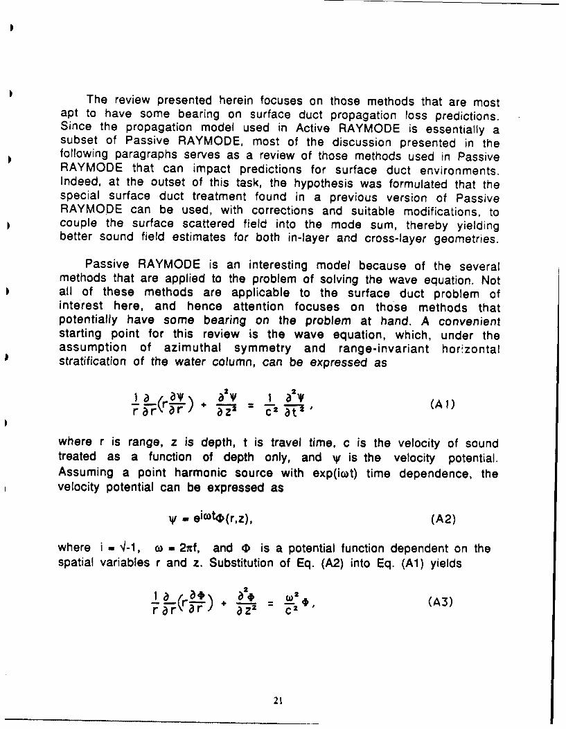
The review presented herein focuses on those methods that are mostapt to have some bearing on surface duct propagation loss predictions.Since the propagation model used in Active RAYMODE is essentially asubset of Passive RAYMODE, most of the discussion presented in thefollowing paragraphs serves as a review of those methods used in PassiveRAYMODE that can impact predictions for surface duct environments.Indeed, at the outset of this task, the hypothesis was formulated that thespecial surface duct treatment found in a previous version of PassiveRAYMODE can be used, with corrections and suitable modifications, tocouple the surface scattered field into the mode sum, thereby yieldingbetter sound field estimates for both in-layer and cross-layer geometries.

Passive RAYMODE is an interesting model because of the severalmethods that are applied to the problem of solving the wave equation. Notall of these methods are applicable to the surface duct problem ofinterest here, and hence attention focuses on those methods thatpotentially have some bearing on the problem at hand. A convenientstarting point for this review is the wave equation, which, under theassumption of azimuthal symmetry and range-invariant hor~zontalstratification of the water column, can be expressed as

where r is range, z is depth, t is travel time, c is the velocity of soundtreated as a function of depth only, and V is the velocity potential.Assuming a point harmonic source with exp(iot) time dependence, thevelocity potential can be expressed as

'V - eicOtO(r,z), (A2)

where i - 4-1, co - 2af, and 0 is a potential function dependent on thespatial variables r and z. Substitution of Eq. (A2) into Eq. (Al) yields

Iar(a) a = (A3)

21

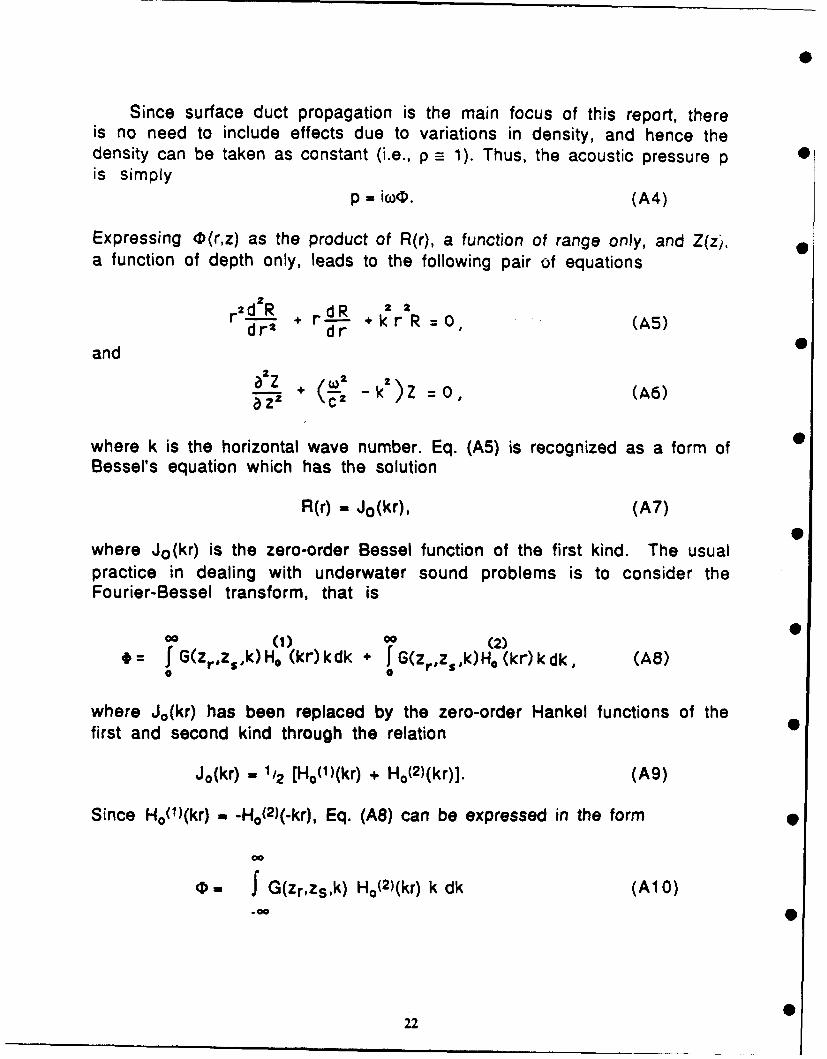
Since surface duct propagation is the main focus of this report, thereis no need to include effects due to variations in density, and hence thedensity can be taken as constant (i.e., p = 1). Thus, the acoustic pressure pis simply

p -iW(. (A4)

Expressing D(r,z) as the product of R(r), a function of range only, and Z(z),a function of depth only, leads to the following pair of equations

r 2 d 2R + rj 2dr + rdR + R =0, (A5)r' dr kr

and

ak )z = 0, (A6)

where k is the horizontal wave number. Eq. (A5) is recognized as a form ofBessel's equation which has the solution

R(r) . Jo(kr), (A7)

where Jo(kr) is the zero-order Bessel function of the first kind. The usualpractice in dealing with underwater sound problems is to consider theFourier-Bessel transform, that is

00 (1) 00 (2)= J G(ZrZs,k)Ho (kr)kdk + JG(zr,zs,k)H. (kr)kdk, (A8)

0

where Jo(kr) has been replaced by the zero-order Hankel functions of thefirst and second kind through the relation 0

Jo(kr) - 1/2 [Ho()(kr) + Ho(2)(kr)]. (A9)

Since Ho(M)(kr) - -Ho( 2)(-kr), Eq. (A8) can be expressed in the form

OW f G(zr,zsk) Ho(2)(kr) k dk (A10)

.00

22

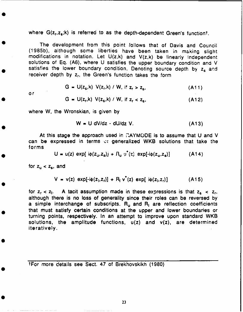
where G(zr,zs;k) is referred to as the depth-dependent Green's functiont.

The development from this point follows that of Davis and Council(1985b), although some liberties have been taken in making slightmodifications in notation. Let U(z,k) and V(z,k) be linearly independentsolutions of Eq. (A6), where U satisfies the upper boundary condition and Vsatisfies the lower boundary condition. Denoting source depth by zs andreceiver depth by zr, the Green's function takes the form

G - U(zs,k) V(zr,k) / W, if Zr > Zs, (All)or

* G - U(Zr,k) V(zs,k) / W, if Zr < Zs, (A1 2)

where W, the Wronskian, is given by

W - U dV/dz - dU/dz V. (A13)

At this stage the approach used in ,,AYMODE is to assume that U and Vcan be expressed in terms cr generalized WKB solutions that take theforms

U - u(z) exp[ io(zu,zs)j + flu u*(z) exp[-io(zu,zs)] (A14)

for zu < zs, and

V - V(Z) exP[-i¢(zl,Zr)] + R, v(z) exp[ iO(zl,Zr)] (Al 5)

for Zr < zj. A tacit assumption made in these expressions is that z. < Zr,although there is no loss of generality since their roles can be reversed bya simple interchange of subscripts. Ru and R, are reflection coefficientsthat must satisfy certain conditions at the upper and lower boundaries orturning points, respectively. In an attempt to improve upon standard WKBsolutions, the amplitude functions, u(z) and v(z), are determinediteratively.

tFor more details see Sect. 47 of Brekhovskikh (1980)

23

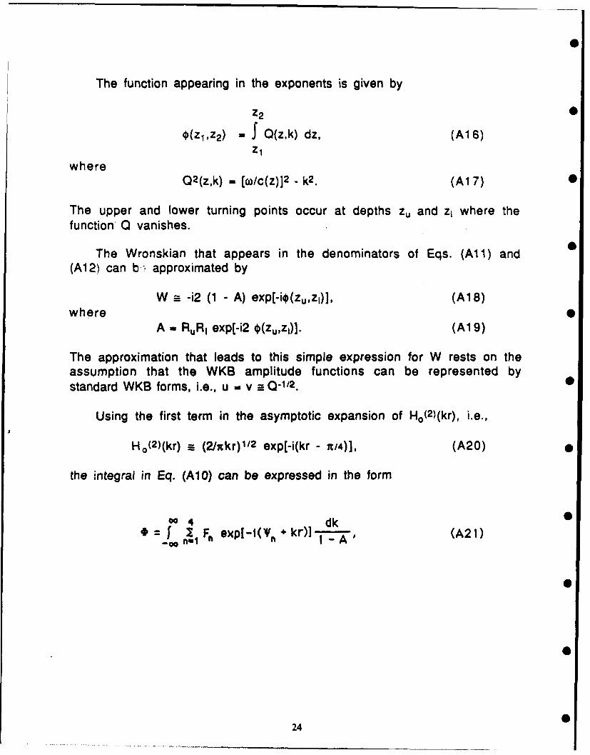
The function appearing in the exponents is given by

z2

-(ZI,Z2) J Q(z,k) dz, (A16)Zl

whereQ2(z,k) - [o/c(z)] 2 - k2 . (Al 7) 0

The upper and lower turning points occur at depths zu and z, where thefunction 0 vanishes.

The Wronskian that appears in the denominators of Eqs. (All) and(A12) can b- approximated by

W -i2 (1 - A) exp[-iO(zu,z1)], (A18)where •

A = RuR I exp[-i2 O(zu,zi)]. (A1 9)

The approximation that leads to this simple expression for W rests on theassumption that the WKB amplitude functions can be represented bystandard WKB forms, i.e., u = v -_-Q1/2. 0

Using the first term in the asymptotic expansion of Ho(2)(kr), i.e.,

Ho( 2)(kr) a (2/xkr) 1/2 exp[-i(kr - R/4)], (A20)

the integral in Eq. (A1O) can be expressed in the form

0dk 4 2I= F exp[-i(V. + kr)] - A (A2 )

24

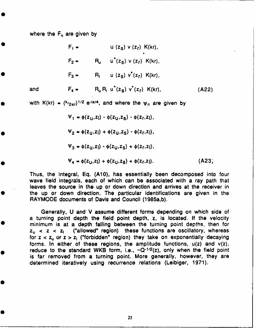
where the Fn are given by

F1 - u (Zs) v (Zr) K(kr),

F2 - Ru U*(Zs) V (Zr) K(kr),

F3 - R, u (Zs) v*(zr) K(kr),

and F4 - Ru R, u*(z s ) v*(zr) K(kr), (A22)

with K(kr) - (k/2xr)l/ 2 e-ix / 4, and where the Wn are given by

V1 - €(Zu,Zl) - O(Zu,Zs) - (Zr,Zl),

V2 - (Zu,Zl) + €(Zu,Zs) - O(Zr,Zl),

'V3 - €(Zu,Zl) - (Zu,Zs) + O(Zr,Zl),

'V4 - (Zu,Zl) + (Zu,Zs) + O(Zr,Zl). (A23;

Thus, the integral, Eq. (A10), has essentially been decomposed into fourwave field integrals, each of which can be associated with a ray path thatleaves the source in the up or down direction and arrives at the receiver inthe up or down direction. The particular identifications are given in theRAYMODE documents of Davis and Council (1985a,b).

Generally, U and V assume different forms depending on which side ofa turning point depth the field point depth, z, is located. If the velocityminimum is at a depth falling between the turning point depths, then forZu < z < z1 ("allowed" region) these functions are oscillatory, whereasfor z < zu or z > zi ("forbidden" region) they take on exponentially decayingforms. In either of these regions, the amplitude functions, u(z) and v(z),reduce to the standard WKB form, i.e., -Q-1 2 (z), only when the field pointis far removed from a turning point. More generally, however, they aredetermined iteratively using recurrence relations (Leibiger, 1971).

25

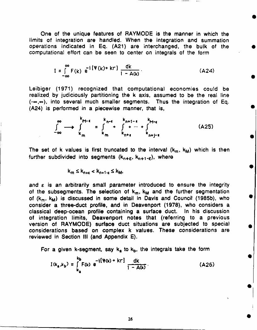
One of the unique features of RAYMODE is the manner in which thelimits of integration are handled. When the integration and summationoperations indicated in Eq. (A21) are interchanged, the bulk of thecomputational effort can be seen to center on integrals of the form

0 =-i IV (k)+ kr] dkI 1F - AN) (A24)

Leibiger (1971) recognized that computational economies could berealized by judiciously partitioning the k axis, assumed to be the real line(-o,.), into several much smaller segments. Thus the integration of Eq.(A24) is performed in a piecewise manner, that is,

,0 ko kM- k n-4 kn I k M-4

f f f + f + + f (A25)-W km km kn+1 kn+J- i

The set of k values is first truncated to the interval (km , kM) which is thenfurther subdivided into segments (kn+e, kn+l-e), where

km < kn+e < kn+l.e <5 kM,

and e is an arbitrarily small parameter introduced to ensure the integrityof the subsegments. The selection of km, kM and the further segmentationof (kin, kM) is discussed in some detail in Davis and Council (1985b), whoconsider a three-duct profile, and in Deavenport (1978), who considers aclassical deep-ocean profile containing a surface duct. In his discussionof integration limits, Deavenport notes that (referring to a previousversion of RAYMODE) surface duct situations are subjected to specialconsiderations based on complex k values. These considerations arereviewed in Section III (and Appendix E).

For a given k-segment, say ka to kb, the integrals take the formkb -l[(k) + kr] dk

I(kakb) [ F(k) S 1 - A(k) (A26)ka

26•

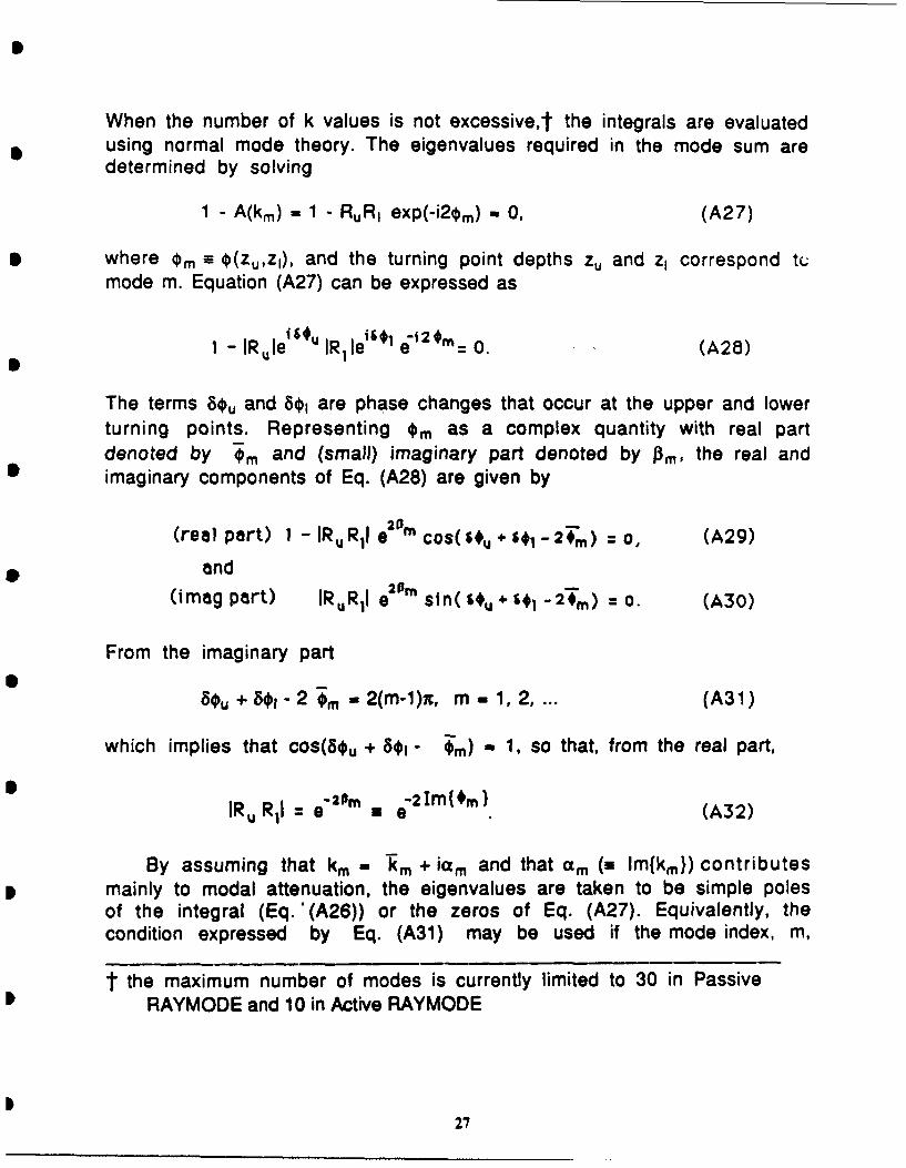
When the number of k values is not excessivet the integrals are evaluatedusing normal mode theory. The eigenvalues required in the mode sum aredetermined by solving

1 - A(km) - 1 - RuRi exp(-i2om) - 0, (A27)

where om a 0(zu,z1 ), and the turning point depths zu and z, correspond tQmode m. Equation (A27) can be expressed as

1 -JRuIeio u IRIle i $ e-i2#m= 0. (A28)

The terms Sou and 80, are phase changes that occur at the upper and lowerturning points. Representing *m as a complex quantity with real partdenoted by *m and (small) imaginary part denoted by A3m, the real andimaginary components of Eq. (A28) are given by

(real part) 1 - IRU Rll e2 0" cos( s* u + 6#1 - 2n) = o, (A2g)

and(imag part) IRURI si n ( OU + 4+1 - 21m) = 0. (A30)

From the imaginary partSou + 85,- 2 Om - 2(m-1)x, m 1, 2, (A31)

which implies that cos(8ou + Sol- Om) - 1, so that, from the real part,

IRU RI = 9'2M a -21m(#m) (A32)

By assuming that km -km + Jam and that am (a lm{km}) contributesmainly to modal attenuation, the eigenvalues are taken to be simple polesof the integral (Eq. '(A26)) or the zeros of Eq. (A27). Equivalently, thecondition expressed by Eq. (A31) may be used if the mode index, m,

t the maximum number of modes is currently limited to 30 in PassiveRAYMODE and 10 in Active RAYMODE

27

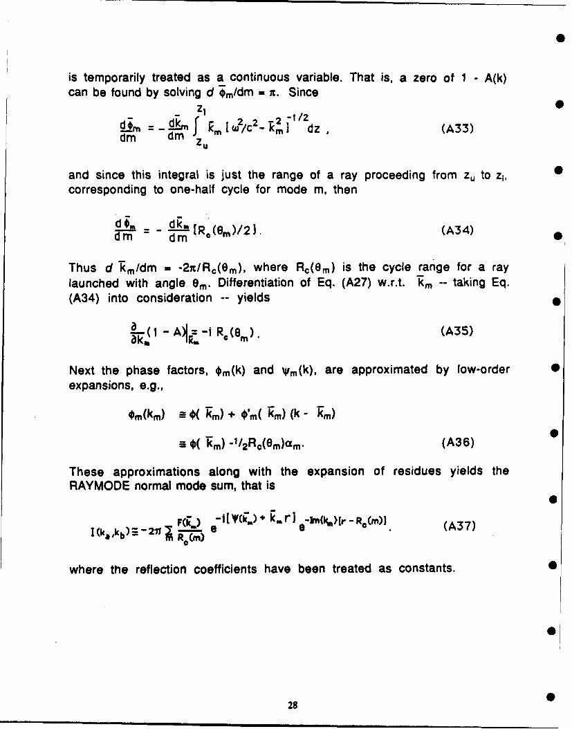
is temporarily treated as a continuous variable. That is, a zero of 1 - A(k)can be found by solving d im/dm - x. Since

- Z_ I 0d- c d 2 -/

=mkm dz , (A33)dm - din Zu

and since this integral is just the range of a ray proceeding from zu to zi,

corresponding to one-half cycle for mode m, then

d -'a d [R (er)/2 . (A34)

Thus d km/dm - "27t/Rc(Om), where Rc(em) is the cycle range for a raylaunched with angle em. Differentiation of Eq. (A27) w.r.t. km -- taking Eq.(A34) into consideration -- yields

a-(I - A .F: -i Re (8. (A35)akakf r

Next the phase factors, *m(k) and vrm(k), are approximated by low-orderexpansions, e.g.,

*m(km) a 0( Wm) + O'm( km) (k - km)

( m) -1/ 2Rc(Om)a m. (A36)

These approximations along with the expansion of residues yields theRAYMODE normal mode sum, that is

r(k',)e - [ Vk. k, r ] e-l~ka r - R (m)].(A 7

S(ka ,b) 211 ; RO/WR

A(37)

where the reflection coefficients have been treated as constants. 0

28

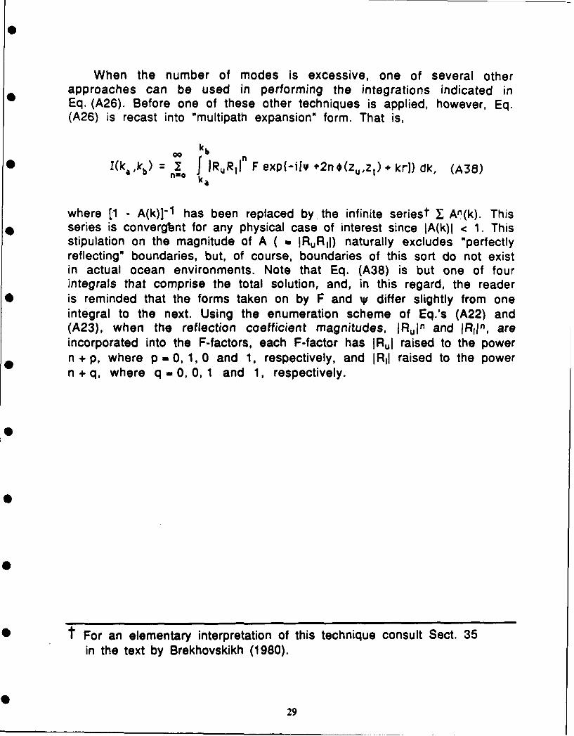
When the number of modes is excessive, one of several otherapproaches can be used in performing the integrations indicated inEq. (A26). Before one of these other techniques is applied, however, Eq.(A26) is recast into "multipath expansion" form. That is,

00 kb

*(kaOkb) = I f IRURII F exp(-i[f +2n#(zu,z ) + kr]) dk, (A38)nIO ka

where [1 - A(k)] "1 has been replaced by the infinite seriest I An(k). Thisseries is convergbnt for any physical case of interest since IA(k)l < 1. Thisstipulation on the magnitude of A ( a IRuRI) naturally excludes "perfectlyreflecting" boundaries, but, of course, boundaries of this sort do not existin actual ocean environments. Note that Eq. (A38) is but one of fourintegrals that comprise the total solution, and, in this regard, the readeris reminded that the forms taken on by F and V' differ slightly from oneintegral to the next. Using the enumeration scheme of Eq.'s (A22) and(A23), when the reflection coefficient magnitudes, IRuI n and lR1ln , areincorporated into the F-factors, each F-factor has IRuj raised to the powern + p, where p -0, 1, 0 and 1, respectively, and IRIJ raised to the powern + q, where q - 0, 0, 1 and 1, respectively.

t For an elementary interpretation of this technique consult Sect. 35in the text by Brekhovskikh (1980).

29

Appendix BSpecial RAYMODE Integration Methods

S3

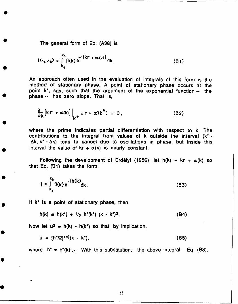
The general form of Eq. (A38) is

kb -t[kr + M(k)]I(ka~kb) f P(k)e dk. (B1)

0 ka

An approach often used in the evaluation of integrals of this form is themethod of stationary phase. A point of stationary phase occurs at thepoint k*, say, such that the argument of the exponential function -- thephase -- has zero slope. That is,

57 k kr + c*)II r + C(k) 0, (132)kk*

where the prime indicates partial differentiation with respect to k. Thecontributions to the integral from values of k outside the interval (k' -Ak, k* - Ak) tend to cancel due to oscillations in phase, but inside thisinterval the value of kr + ct(k) is nearly constant.

Following the development of Erdelyi (1956), let h(k) - kr + cz(k) sothat Eq. (B1) takes the form

_ kb -l h(k)I= f P(k)e dk. (13)

ka

If k* is a point of stationary phase, then

h(k) h(k*) + 1/2 h"(k °) (k - k*)2. (B4)

Now let u2 - h(k) - h(k*) so that, by implication,

u - [h-/211' 2 (k - k*), (B5)

where h" a hw(k)lk. With this substitution, the above integral, Eq. (B3),

33

becomes

u ei[h(k) + du. (16)

Uj

In the neighborhood of k*, 13(k) -+ 0(k*) and 2u/h'(k) assumes. an 0

indeterminate form. Applying L'Hospital's rule

2u/h'(k) - 2u'/h"(k) (B7)

which as k - k* evaluates to (k - k*)/u = (2/h")1/2, and this result in turn

implies that the largest acceptable value for Ak is (2/h") 1/2. Thus, theintegral in Eq. (B6) reduces to

I= 1(k * )' e -ih(k*)J eitU~du. (B8)U2

The variable of integration chosen for RAYMODE is obtained by settingy- (2/)1/2u, so that Eq. (B8) becomes

i P(k)V/ (k el~k* +)+k*rIfeuIS du, (B9)

which, of course, requires that a"(k) does not become vanishingly small ask -+ k*.

When the point of stationary phase falls outside the segment (ka,kb),the phase function is expanded about the end-point closest to k*. In thiscase, the Taylor series expansion contains a first-derivative term, butthrough a suitable transformation the integrand is cast in the same formas the one in Eq. (B9). Thus, in both the illuminated case, k* e (ka,kb), Sand in the shadow case, k* e (ka,kb), the integral that has to be

34

evaluated takes the form

I =f, /2dy. (B 10)

I This integral can be expressed in terms of the Fresnel integrals, that is,

I - C(Y2) - C(YI) - i[S(Y2 ) - S(y)], (Bl1)where

S 2c(r) oCSx dx, (B12)

and,

S J j. sin Mx 2 dx. (B13)

The limits of integration depend upon the location of k* relative to theinterval end-points ka and kb. Leibiger (1971) presents a table ofappropriate values of Yi and Y2 under various conditions on ka- k* andkb -k.

The special high frequency integration (HFI) method is essentially anextension of the original RAYMODE integration (ORI) method. As shown inSect. 45 of Brekhovskikh (1980), when a"(k) is finite the integral, Eq.(B1), evaluates to the "saddle point formula" given by

- [ ( k* ) ± n,/4JI = I/'(k:ll p(k) e (B 14)

where the sign in the exponent agrees with the sign of az(k*). When

Ia"(k) < e, for some small e > 0, the evaluation point (r,z), say, is veryclose to a caustic -- an indication that special handling is required. Tocover all possibilities the phase factor, a(k) + kr, is expanded to anadditional term, i.e.,

a(k) + kr S a(k*) + k*r + (a' +r)(k - k*)

+ a"(k - k*)2/2 + a"'(k - k*)3/6, (B15)

35

where the derivatives are evaluated at k - k*, and k* is a point ofstationary phase that lies within the interval of integration (ka,kb). Fromthe stationary phase condition, i.e., a' + rIk. - 0, the a-derivatives can beexpressed in terms of the r-derivatives. Let rc denote the value of rangewhen k = k*. Then at k - k*, a' - -rc, a" - -rc ' and a"' . -rc". Making thesesubstitutions and assuming that a" 0 0, Eq. (B15) becomes

a(k) + kr a a(k*) + k*r + (r- rc)(k - k) - rc"(k - k*)3/6. (B16)

Under these conditions the integral, Eq. (B1), can be put into the form

I =3(k*) e-i [a(k) + k'r

X f exp( i[(r - rc)(k - k*) + r,"(k - k*)3/6]). (B17)

Through suitable transformations applied to the variables r - rc and k -k* (see, for example, p.390 in Brekhovskikh, 1980), this integral can be

approximated by an Airy function.

In addition to the extended Taylor series expansion, there are somesubtle differences between this method and the approach taken in the ORImethod. In the "original" method, the derivative r' is determined usingfinite differences, whereas in the "high frequency" method it isdetermined analytically. Finite differencing is used in estimating r"however.

36

Appendix CBreakdown of Phase Factor

37

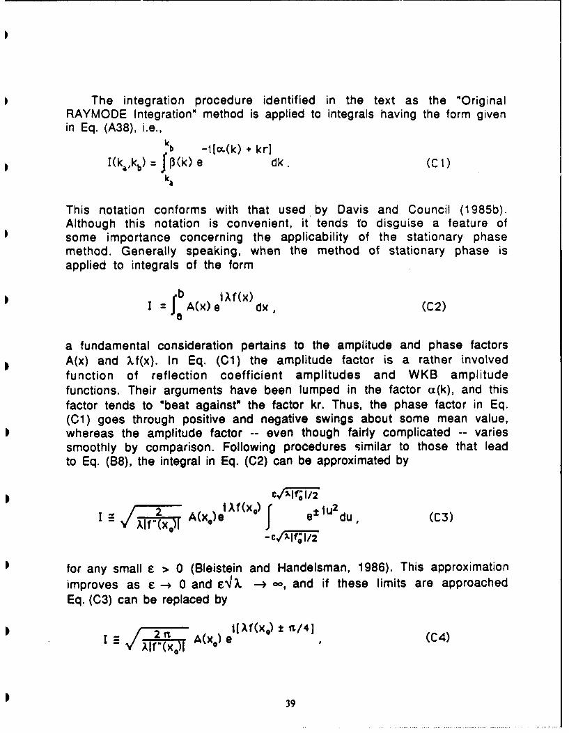
The integration procedure identified in the text as the "OriginalRAYMODE Integration" method is applied to integrals having the form givenin Eq. (A38), i.e.,

k b -i[.(k) + kr]

I(k,,kb) P(k) e dk. (C)ka

This notation conforms with that used by Davis and Council (1985b).Although this notation is convenient, it tends to disguise a feature ofsome importance concerning the applicability of the stationary phasemethod. Generally speaking, when the method of stationary phase isapplied to integrals of the form

i~f(x)

S=f A(x) e dx, (C2)

a fundamental consideration pertains to the amplitude and phase factorsA(x) and Xf(x). In Eq. (Cl) the amplitude factor is a rather involvedfunction of reflection coefficient amplitudes and WKB amplitudefunctions. Their arguments have been lumped in the factor ca(k), and thisfactor tends to "beat against" the factor kr. Thus, the phase factor in Eq.(Cl) goes through positive and negative swings about some mean value,whereas the amplitude factor -- even though fairly complicated -- variessmoothly by comparison. Following procedures similar to those that leadto Eq. (B8), the integral in Eq. (C2) can be approximated by

CVXlIf; 1/2

2 x A(xo)el f l e/2du (C3)

-C,'XIf; 1/2

for any small s > 0 (Bleistein and Handelsman, 1986). This approximationimproves as e -- 0 and e'/; -- 0 and if these limits are approachedEq. (C3) can be replaced by

2fL (IA0) el[I)X) ± i/4] (C4)Xf(x0 IA9

39

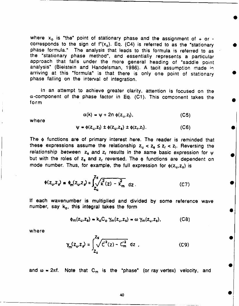
where xo is "the" point of stationary phase and the assignment of + or -corresponds to the sign of f"(xo). Eq. (C4) is referred to as the "stationary 0phase formula." The analysis that leads to this formula is referred to asthe "stationary phase method", and essentially represents a particularapproach that falls under the more general heading of "saddle pointanalysis" (Bleistein and Handelsman, 1986). A tacit assumption made inarriving at this "formula" is that there is only one point of stationaryphase falling on the interval of integration.

In an attempt to achieve greater clarity, attention is focused on thea-component of the phase factor in Eq. (Cl). This component takes theform

a(k) = + 2n O(zu,zj), (C5)where

-O (zuZI) ± O(Zu,Zs) ± O(Zr,Zl). (C6) 0

The 0 functions are of primary interest here. The reader is reminded thatthese expressions assume the relationship zu < zs 5 Zr < z1. Reversing therelationship between zs and Zr results in the same basic expression for Wrbut with the roles of z. and Zr reversed. The 0 functions are dependent onmode number. Thus, for example, the full expression for O(zu,zs) is

Zs

* z m(Z,z J k (z)- km dz (C7) 0ZU

If each wavenumber is multiplied and divided by some reference wavenumber, say k, this integral takes the form 0

Om(Zu,Zs) - koC O 'ym(Zu,Zs) -= c ym(Zu,Zs), (C8)

wherezS 0

(ZUz) J C2(z) _ C dZ (Cg)

zu

and co - 27f. Note that Cm is the "phase" (or ray vertex) velocity, and

40 0

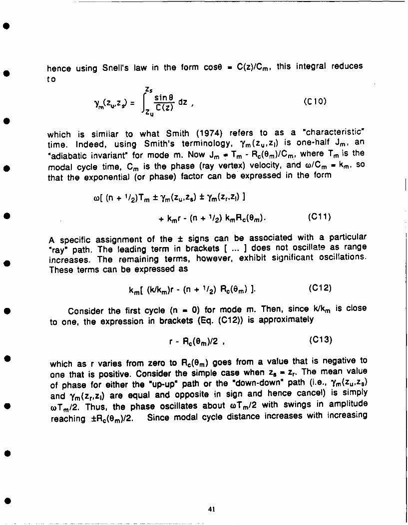
hence using Snell's law in the form cose - C(z)/Cm, this integral reducesto

SZY=Z~ jz sin dz, (CLO0)

which is similar to what Smith (1974) refers to as a "characteristic"

time. Indeed, using Smith's terminology, Ym(Zu,Zl) is one-half Jm, an"adiabatic invariant" for mode m. Now Jm Tm - Rc(Om)/Cm, where Tm is the

modal cycle time, Cm is the phase (ray vertex) velocity, and co/Cm - kin, so

that the exponential (or phase) factor can be expressed in the form

o[ (n + 1/2)Tm ± Ym(Zu,Zs) ± Ym(Zr,Zl) I

+ kmr - (n + 1/2) kmRc(em). (Cl1)

A specific assignment of the ± signs can be associated with a particular"ray" path. The leading term in brackets [ ... ] does not oscillate as range

increases. The remaining terms, however, exhibit significant oscillations.

These terms can be expressed as

km[ (k/km)r - (n + 1/2) Rc(em)]. (C12)

Consider the first cycle (n - 0) for mode m. Then, since k/km is close

to one, the expression in brackets (Eq. (C12)) is approximately

r - Rc(am)/2 , (C13)

which as r varies from zero to Rc(O) goes from a value that is negative to

one that is positive. Consider the simple case when Z. - Zr. The mean value

of phase for either the "up-up" path or the "down-down" path (i.e., Ym(Zu,Zs)

and Ym(Zr,Zl) are equal and opposite in sign and hence cancel) is simply

*)Tm/ 2 . Thus, the phase oscillates about o)Tm/ 2 with swings in amplitude

reaching ±Rc(em)/ 2 . Since modal cycle distance increases with increasing

41

mode number, m, these oscillations become large in magnitude for high-order modes - although their frequency of oscillation becomes less rapid. 0Conversely, osciliations for the low-order modes are not as extensive inmagnitude but they are fairly rapid. In either case the phase variation israpid relative to the amplitude variation, and hence as long as thereference wave number ko (= 2f/Co) is large, i.e., the frequency is "hig",the criteria necessary for Eq. (C4) are met. The validity of Eq. (C3),however, does not necessarily require that ko -* o-. Even for relativelymodest values of ko , as long as the interval of integration is properlyconfined, this integral yields an acceptable approximation. Obviously thereis some frequency below which this method fails. Hopefully the transitionto the RAYMODE "normal mode" sum occurs before that frequency isreached!

4

42S

Appendix DSurface Reflection Loss Submodel

43

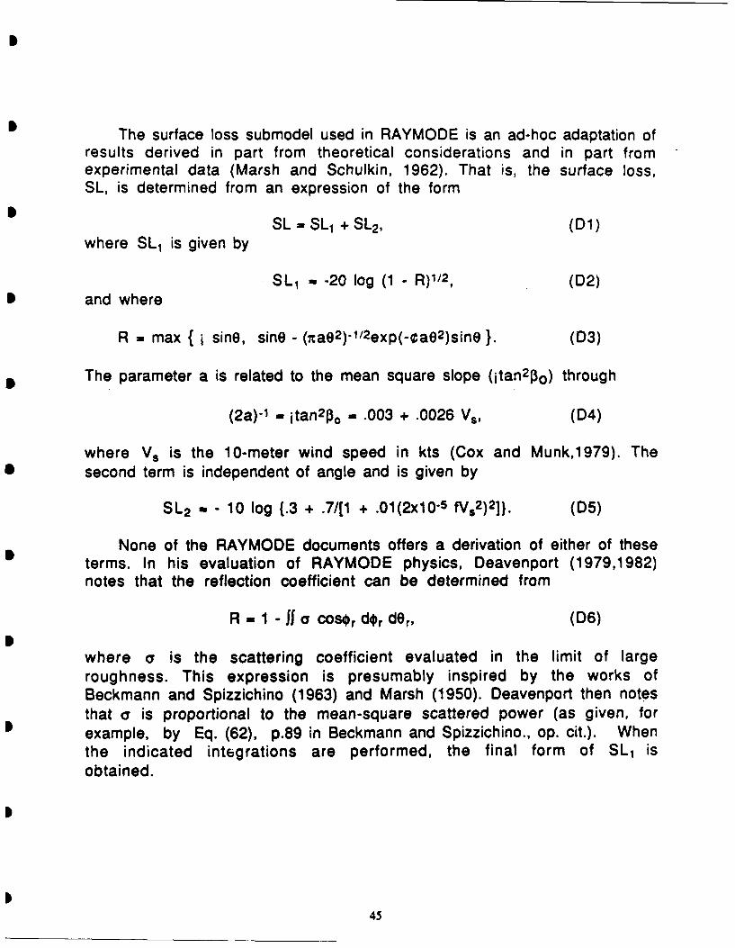
The surface loss submodel used in RAYMODE is an ad-hoc adaptation ofresults derived in part from theoretical considerations and in part fromexperimental data (Marsh and Schulkin, 1962). That is, the surface loss,SL, is determined from an expression of the form

SL = SL 1 + SL2 , (D1)where SL1 is given by

SL1 - -20 log (1 - R) 1/2 , (D2)and where

R - max { i sine, sine - (7rae 2 )-"/2exp(-¢ae2)sine }. (D3)

The parameter a is related to the mean square slope (itan2p3o) through

(2a) -1 - itan2po - .003 + .0026 Vs , (D4)

where Vs is the 10-meter wind speed in kts (Cox and Munk,1979). Thesecond term is independent of angle and is given by

SL 2 - - 10 log (.3 + .7/[1 + .01(2x10- s fVs2 ) 2]}. (D5)

None of the RAYMODE documents offers a derivation of either of theseterms. In his evaluation of RAYMODE physics, Deavenport (1979,1982)notes that the reflection coefficient can be determined from

R - 1 cOSr d r dr, (D6)

where a is the scattering coefficient evaluated in the limit of largeroughness. This expression is presumably inspired by the works ofBeckmann and Spizzichino (1963) and Marsh (1950). Deavenport then notesthat a is proportional to the mean-square scattered power (as given, forexample, by Eq. (62), p.89 in Beckmann and Spizzichino., op. cit.). Whenthe indicated integrations are performed, the final form of SL 1 isobtained.

45

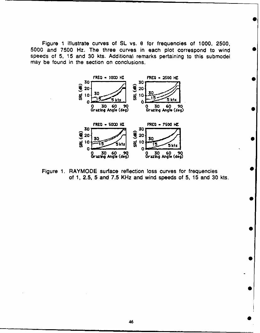
Figure 1 illustrate curves of SL vs. 0 for frequencies of 1000, 2500,5000 and 7500 Hz. The three curves in each plot correspond to windspeeds of 5, 15 and 30 kts. Additional remarks pertaining to this submodelmay be found in the section on conclusions.

% REO a 1OU0 HZ FREQ - SOa IW .

20 1o20...- C, I=l30 0I o

0 i ts ts0 30 60 90 0 30 60 90Grazing Anglo (dog) Grazing Angle (dog) 0

rREo -S 0 NZQ -7OIHZo 30 30

30 6 30 05 k15

S30 60 Q 30 60 90zing Anglo (dig) arazing Anglo (dog)

Figure 1. RAYMODE surface reflection loss curves for frequencies 0

of 1, 2.5, 5 and 7.5 KHz and wind speeds of 5, 15 and 30 kts.

0

0

0

0

46 0

Appendix EComplex Elgenvalues

S4

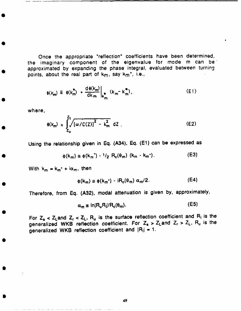
Once the appropriate "reflection" coefficients have been determined,the imaginary component of the eigenvalue for mode m can beapproximated by expanding the phase integral, evaluated between turningpoints, about the real part of kin, say kin*, i.e.,

+ d(*k (km k*)''. (El)

where,Z1 C ~ 22

*(km) = J/[w/C(Z)] 2 - km dZ (E2)Zu

Using the relationship given in Eq. (A34), Eq. (El) can be expressed as

*(km) =- O(km') - '/2 Rc(em) (km - kin). (E3)

With km - km + iam, then

0(km) = (km) - iRc(om) cam/2. (E4)

Therefore, from Eq. (A32), modal attenuation is given by, approximately,

am a InIRuRij/Rc(em). (E5)

For Z. < ZLand Zr < ZL, Ru is the surface reflection coefficient and R, is the

generalized WKB reflection coefficient. For Z. > ZLand Zr > ZL, Ru is the

generalized WKB reflection coefficient and IRI1 - 1.

49

Appendix FDeparture of n 2-linear Profile Model from Linearity

0

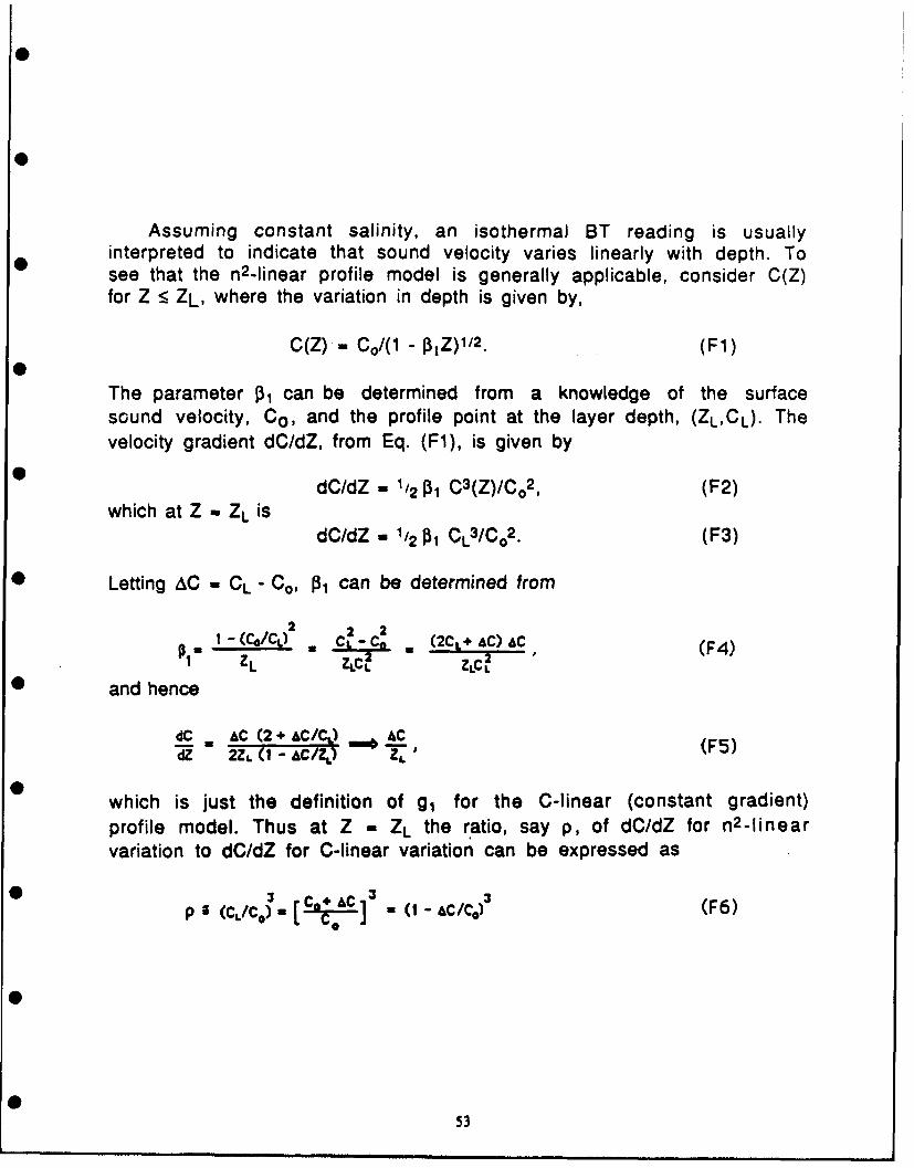
0

Assuming constant salinity, an isothermal BT reading is usuallyinterpreted to indicate that sound velocity varies linearly with depth. Tosee that the n2 -linear profile model is generally applicable, consider C(Z)for Z 5 ZL, where the variation in depth is given by,

C(Z) - Co/(1 - 1/Z) .'2 (Fl)

The parameter 13, can be determined from a knowledge of the surfacesound velocity, C o , and the profile point at the layer depth, (ZL,CL). Thevelocity gradient dC/dZ, from Eq. (Fl), is given by

dC/dZ - 1/2 13 C3(Z)/C 0 2, (F2)which at Z - ZL is

dC/dZ - 1/2 1 CL3 /Co2 . (F3)

Letting AC - CL - CO, 13i can be determined from

,1 -(c/c 1) ____ ___

ZC -Ca (2CL+ Ac) c(F4)I3L ZLC L zLC L *(

and hence

dC C (2 + AC/C AC (dZ " 2Z (! - /N

which is just the definition of g, for the C-linear (constant gradient)profile model. Thus at Z - ZL the ratio, say p, of dC/dZ for n2-linearvariation to dC/dZ for C-linear variation can be expressed as

P a (£ C [- O'] -(I- Ac/C) : (F6)

00

53

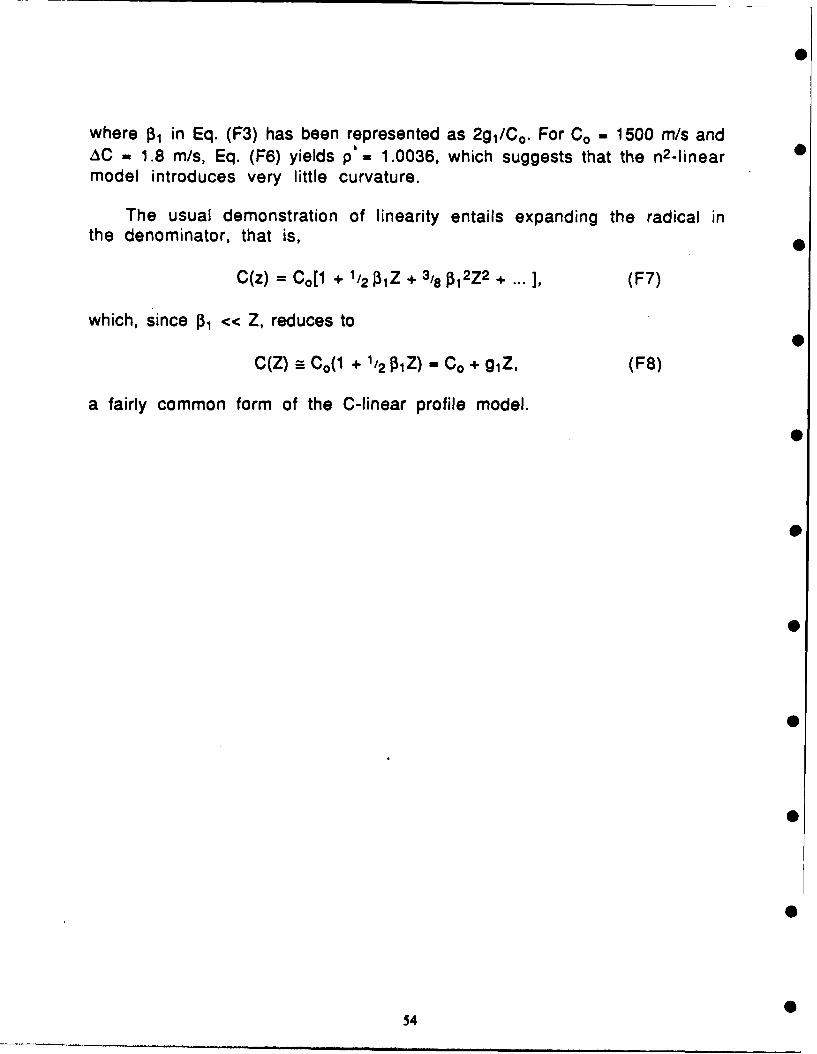
where 3, in Eq. (F3) has been represented as 2g1/Co. For Co - 1500 m/s andAC - 1.8 m/s, Eq. (F6) yields p - 1.0036, which suggests that the n2-linearmodel introduces very little curvature.

The usual demonstration of linearity entails expanding the radical inthe denominator, that is,

C(z) = Co[1 + 1/2 P1Z + 3/8 p12 Z 2 + ... ], (F7)

which, since 13i << Z, reduces toC(Z) = Co(1 + 1/2PIZ) - CO + 1Z, (F8)

a fairly common form of the C-linear profile model.

0

540

I

Appendix GModal Parameters for a C3 -linear Duct

I

I

I

p

I

p

p

I

I55

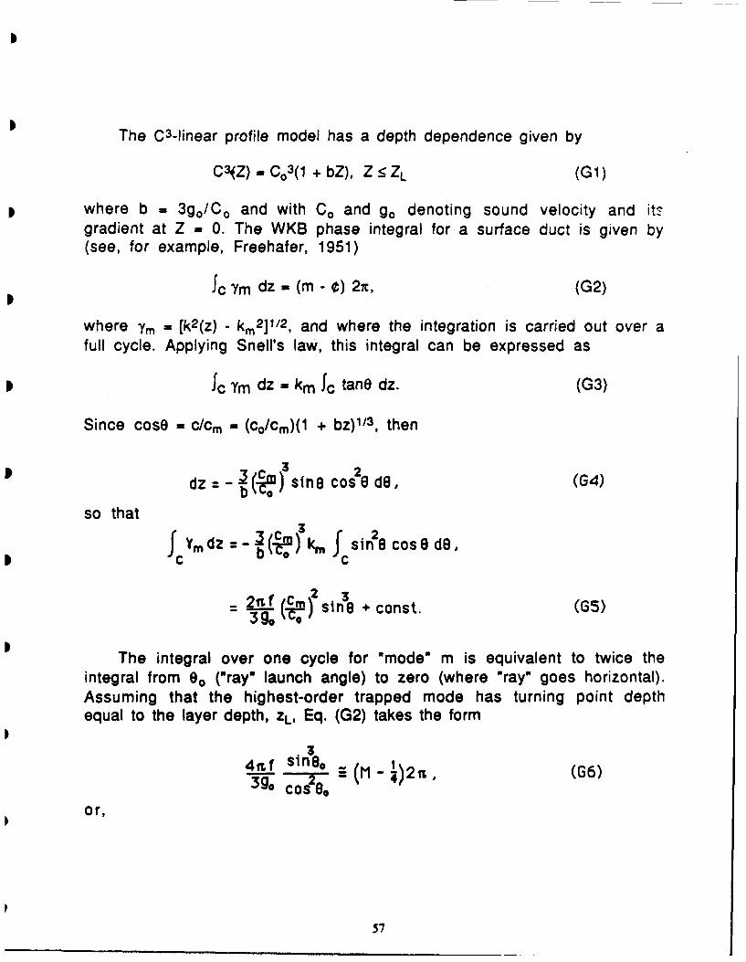
The C3-linear profile model has a depth dependence given by

C3Z) . C0 3(1 + bZ), Z _< ZL (Gi)

0 where b = 3go/C o and with Co and go denoting sound velocity and itlgradient at Z - 0. The WKB phase integral for a surface duct is given by(see, for example, Freehafer, 1951)

JC ym dz - (m - ¢) 2n, (G2)

where ym - (k2(z) - km2]"/2 , and where the integration is carried out over afull cycle. Applying Snell's law, this integral can be expressed as

0 'c Ym dz - km 'c tanO dz. (G3)

Since cose - c/cm - (co/cm)(1 + bz) 113 , then

dz =- - ~(~sine cos 8 d6, (G4)

so that

fr Ydz ~(Wkm fln 8 cos 8 d8,

W C. 2 sine + const. (G5)

The integral over one cycle for "mode" m is equivalent to twice theintegral from 00 ("ray" launch angle) to zero (where "ray" goes horizontal).Assuming that the highest-order trapped mode has turning point depthequal to the layer depth, zL, Eq. (G2) takes the form

3

3go = q (M - )2nL (G6)

or,

57

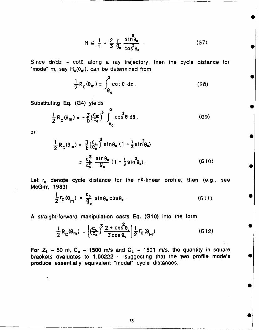
0

.3M + f-s neo (G7)1 3_ 2 lfB

~ ~g 0 Cos~e (G0

Since dr/dz = cotO along a ray trajectory, then the cycle distance for"mode" m, say Rc(Om), can be determined from

o•

I R (8m~ = cot 8 dz. (Ga)eo

Substituting Eq. (G4) yields02R (em~ c)---o r cos36 de, (G9)

or,

S2 no)

= J . o (sineo (I ISn 2eg). (GIO0)

Let rc denote cycle distance for the n2 -linear profile, then (e.g., seeMcGirr, 1983)

1 co- slneo coseo. (G 1 1)

A straight-forward manipulation casts Eq. (GIO) into the form

3 21 )2 + cos 80 lrc(9) (G12)Tc(em) 3cosq 2 eoM

For ZL - 50 m, Co - 1500 m/s and CL - 1501 m/s, the quantity in squarebrackets evaluates to 1.00222 -- suggesting that the two profile models 0produce essentially equivalent "modal" cycle distances.

58

Appendix HBucker's Scattering Integrals

0

05

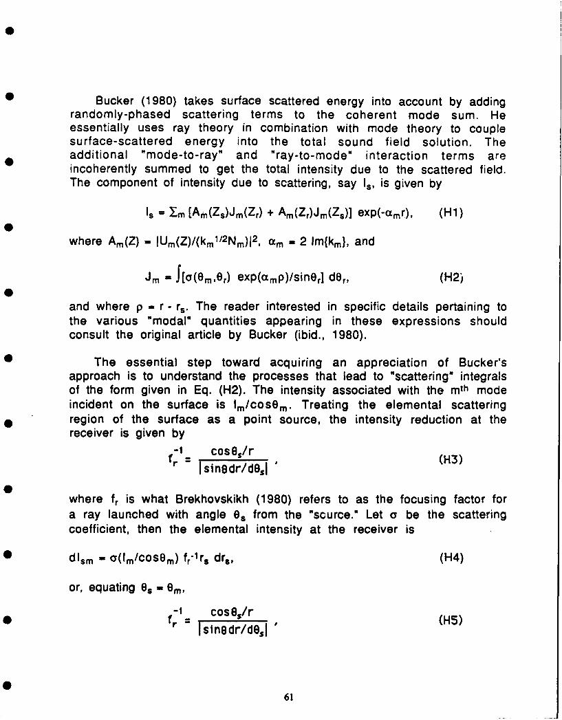
Bucker (1980) takes surface scattered energy into account by addingrandomly-phased scattering terms to the coherent mode sum. Heessentially uses ray theory in combination with mode theory to couplesurface-scattered energy into the total sound field solution. Theadditional "mode-to-ray" and "ray-to-mode" interaction terms areincoherently summed to get the total intensity due to the scattered field.The component of intensity due to scattering, say Is , is given by

Is= -Xm [Am(Zs)Jm(Zr) + Am(Zr)Jm(Zs)] exp(-amr), (H1)

where Am(Z) = IUm(Z)/(km"12 Nm)12 , am . 2 Im{km), and

J J[(Om,Or) exp(amp)/sin0r] dOr, (H2)

and where p = r - rs. The reader interested in specific details pertaining tothe various "modal" quantities appearing in these expressions shouldconsult the original article by Bucker (ibid., 1980).

The essential step toward acquiring an appreciation of Bucker'sapproach is to understand the processes that lead to "scattering" integralsof the form given in Eq. (H2). The intensity associated with the mth modeincident on the surface is Im/cosOm. Treating the elemental scatteringregion of the surface as a point source, the intensity reduction at thereceiver is given by

- cose,/rr - Isinedrd l (

where fr is what Brekhovskikh (1980) refers to as the focusing factor fora ray launched with angle Os from the "source." Let a be the scatteringcoefficient, then the elemental intensity at the receiver is

dlsm - a(Im/cosOm) fr'lrs drs, (H4)

or, equating 0. - Om,

- coses/r (15)r = Isinedr/deI(

61

Bucker (1980) expresses Im in terms of modal quantities, i.e.,

Im - (2n/rs) Am(zo) exp(-amrs), (H6)

and then integrates Eq. (H5) to get

Ism - (2ic/r) Am(zo)Jm(z)exp(-amr), (H7)

where Jm(z) -- not to be confused with a Bessel function -- is given byEq. (H2). The limits of integration are defined as the limiting values of theset of rays that directly connect the surface and either the source or thereceiver. That is, there are actually two interaction (or scattering)integrals. Near the source, rays propagate energy to the rough surface,whereupon the incoherent component of the surface scattered energy givesrise to normal modes which continue the propagation of waves toward thereceiver. This interactive effect represents a ray-to-mode exchange ofenergy. Near the receiver, the energy associated with a given mode isscattered by the rough surface, whereupon the incoherent component ofthe surface scattered energy gives rise to rays that propagate energy fromthe surface to the receiver. This interactive effect represents a mode-to-ray exchange of energy. The details of this procedure are omitted here butmay be found in the report by Gordon and Bucker (1984). 0

In his original article, Bucker (1980) assumes that the specularsurface reflection coefficient, Sm, is given by

Sm - -exp(-gm/2). (HS)

The parameter gm, referred to as the Rayleigh roughness parameter, isdefined as (e.g., see p. 82 in Beckmann and Spizzichino, 1963)

gm- (2k h sinOsm) 2, (H9)

where ks = o/Cs, esrn is the surface grazing angle of incidence for the mthmode, and h is the rms surface roughness. He also assumes Lambert's law(Houston, 1915) which, when the energy lost to specular reflection istaken into account, results in the following expression for a:

O(em,,) - 1/2 (1 - ISmI2) sine,. (H10)

62

Distribution List

Asst Secretary of the Navy Commanding Officer University of California(Research, Engineering & Systems) Naval Research Laboratory Scripps Institute of OceanographyNavy Department Washington DC 20375 Marine Physical LaboratoryWashington DC 20350-1000 Director P.O. Box 6049

DResrch LSan Diego CA 92106Chief of Naval Operations Naval Research Laboratory Attn: W. HodgekissNavy eparmentWashington DC 20375Navy Department Attn: Code 5160, W. KupermanWashington DC 20350-1000 Officer in ChargeAttn: OP-02 Commander Naval Surface Weapons Center Det

OP-71 Naval Oceanography Command White Oak LaboratoryOP-0962X, R. Feden Stennis Space Center MS 39529-5000 10901 New Hampshire Ave.OP-987 Attn: Code N31, CDR F. Zelie Silver Spring MD 20903-5000

Commanding Officer Attn: Code U31, R. AhlbergFleet Numerical Oceanography Center Library

Chief of Naval Operations Monterey CA 93943-5005U.S. Naval Observatory Attn: LCDR Braunstein Commanding Officer34th & Mass Ave., NW LCDR Hall Fleet Anti-Sub Warfare Training Center,Washington DC 20390-1800 LCDR Tompkins AtlanticAttn: OP-96 Naval Station

Commanding Officer Norfolk VA 23511-6495Commander Naval Oceanographic OfficeNaval Air Development Center Stennis Space Center MS 39522-5001 Defense Mapping Agency Sys CenWarminster PA 18974-5000 Attn: Code GGAP, B. Mullen 12100 Sunset Hill Rd. #200Attn: Code 3031, C. L. Bartberger Code A, J. Depner Reston VA 22090-3207

Code 7300, W. Jobst Attn: SGWNCommanding Officer Code 9200, L. Bernard Code 1ODI10P, Dr. E. SilvaNaval Coastal Systems Center Code 9210, A. Crumpler Mel WagnerPanama City FL 32407.5000 Commander Ed Danford

Naval Ocean Systems CenterCommander San Diego CA 92152-5000 Office of Naval TechnologySpac;e & Naval Warfare Sys Coin Attn: Code 541, H. Buckner 800 N. Quincy St.Washington DC 20363-5100 Code 541, F. Ryan Arlington VA 22217-5000Attn: Code 361, J. Reeves Attn: Code 20, Dr. P. Selwyn

Commanding Officer Code 228, Dr. M. BriscoeCommanding Officer ONR Branch Office Code 234, Dr. C. V. VotawNaval Environmental Prediction Box 39Research Facility FPO New York NY 09510-0700 Office of Naval ResearchMonterey CA 93943-5006 Commander 800 N. Quincy St.

David W. Taylor Naval Research Center Arlington VA 22217-5000Commander Bethesda MD 20084-5000 Attn: Code 10Naval Facilities Eng Command Code 1OD/10P, Dr. E. SilvaNaval Facilities Eng Command HO Commander Code 12200 Stovall St. Naval Surface Weapons Center Code 112, Dr. E. HartwigAlexandria VA 22332-2300 Dahlgren VA 22448-5000 Code 125, K. W. Lackie

Attn: LibraryCommanding Officer Commanding Officer CommanderNaval Ocean R&D Activity Naval Underwater Systems Center Naval Sea Systems CommandStennis Space Center MS 39529-5004 Newport RI 02841-5047 Naval Sea Systems Command HOAttn: Code 100 Washington DC 20362-5101

Code 105 Superintendent Attn: Code 63D3, P. TiedemanCode 110 Naval Postgraduate School Code PMS 411, Dr. E. EstaloteCode 112 Monterey CA 93943 Code 63R14, A. FranceschettiCode 113 Attn: H. Medwin (Dept.IPhysics)Code 114 C. Dunlap, (Dept.JOceanography) Commanding OfficerCode 115 DNaval Civil Engineering LaboratoryCode115Director of Navy Laboratories Port Hueneme CA 93043Code 117, J. Hammack Rm 1062, Crystal Plaza Bldg 5Code 125EX Department of the Navy CommanderCode 125L (13) Washington DC 20360Code 125P (1) Naval Air Systems CommandCode 200 Officer in Charge Naval Air Systems Command HO

Code 210 New London Laboratory Washington DC 20361-0001Code 211 Naval Underwater Sys Cen DetCode 220 New London CT 06320 Pennsylvania State University

Code 221 (5) Attn: Code 33A, B. Cole Applied Research LaboratoryCode 222 (3) Code 33A3, P. Herstein P.O. Box 30Code 223 (6) Code 3342, D. Lee State College PA 16801Code 224 (3) Code 6091, J. Doebler

Code 240 Code 6091, R. Almeida University of Texas at Austin

Code 244 Code 3342, R. Deavenport Applied Research Laboratories

Code 245 G. Leibiger P.O. Box 8029

Code 300 Austin TX 78713-8029Code 30,.Hika DirectorCode 350, D. Hickman National Ocean Data Center Johns Hopkins UniversityCode 351, J. Braud WSC1 Room 103 Applied Physics LaboratoryCode 351, M. Lohrenz 6001 Excutive Blvd. Johns Hopkins Rd.

Rockvllle MD 20852 Laurel MD 20707Brooke Farquhar Attn: G. W. Withee

NORDA Liaison Office Director University of WashingtonCrystal Plaza #5, Room 802 Woods Hole Oceanographic Inst Applied Physics Laboratory2211 Jefferson Davis Hwy. P.O. Box 32 1013 Northeast 40th St.Arlington VA 22202-5000 Woods Hole MA 02543 Seattle WA 98105

Office of Naval Research Science Applications SYNTEK Engineering & ComputerField Detachment International, Corp. Systems, Inc.Stennis Space Center MS 39529 PO Box 2351 2600 Garden RoadAttn: Code 125, E. Chaika LaJolla CA 92038 Suite 202

Monterey CA 93940Commander Science Applications Attn: N. GreenfetdtSubmarine Development Squadron 12 International, Corp.Box 70 1710 Goodridge Drive Defence Scientific EstablishmentNaval Submarine Base PO Box 1303 HMNZ DockyardNew London McLean VA 22102 Devonport, AucklandGroton CT 06340 Attn: Dr. A. Eller New ZealandGroto CT 6340Attn: R. Bannister

SYNTEK Engineering & Computer D. KewleyR. E. (Ruth) Keenan Systems, Inc.c/o Associated Scientists 2101 East Jefferson Street Defense Technical Information Co":erBox 721 Suite 300 Cameron Station (12)Woods Hole MA 02543 Attn: B. Scaife Alexandria VA 22314

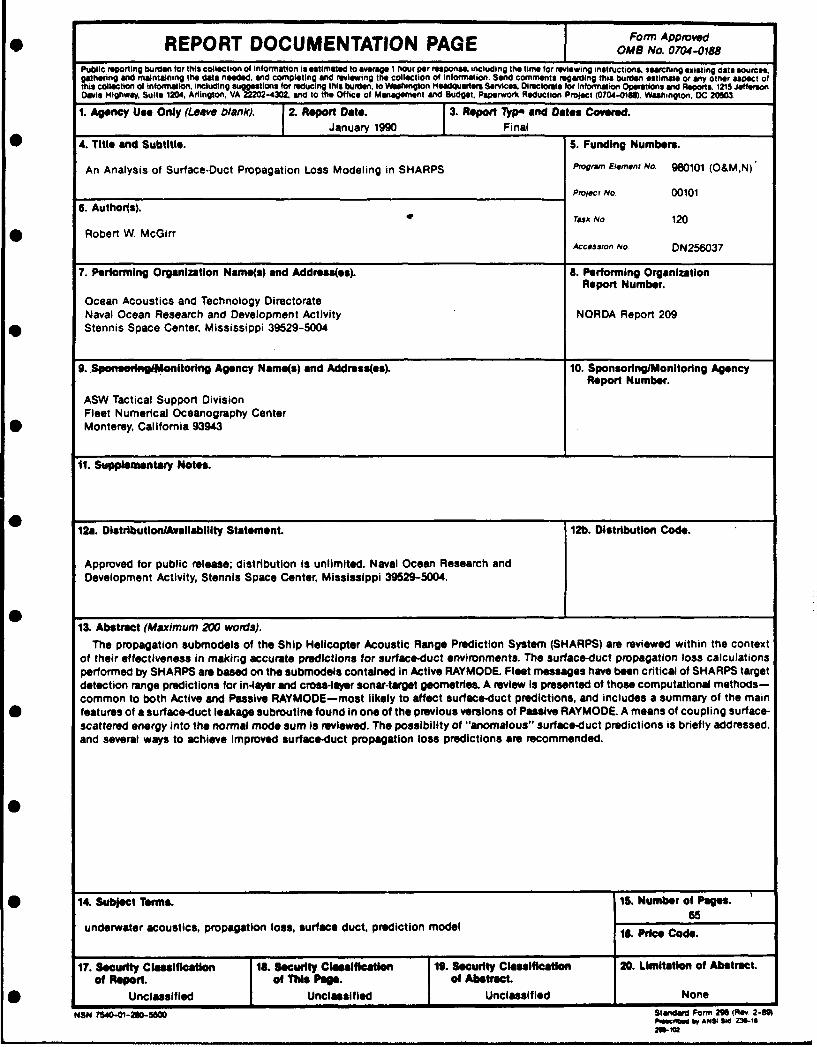
I Form ApprovedREPORT DOCUMENTATION PAGE j oMB No. 07oiUI", No. 0Sou-ces

Public.reporling burden for this collection of information isl estimated to avrag~e 1 hour per responsei including the time for reviewirng intructions.k searching existing dats sourcesgathering and maintaining the data needed, ando completing an reviewing the collection of information. Send comments regarding thisl burden estimate or any other aspect ofthie Collec¢tion of information, including sluggs~etionsl for reducing this burdenll to Wuhngton Meedquwters Seices. Directorate for Informnation 0Operationsl and Reports 1215 JeffersonODavis Highway. Suite 1204, Arlington, VA 22202-4302, sn to the Office of Management and Budget, Paperwork Reduction Proect (0704-018). Washington. DC 20803

1. Agency Us. Only (Leave blank). 2. Report Date. 3. Repor l~vp. and Dites Covered.I January 1990 IFinal

*4. Title and Subtitle. 5. Funding Numbers.

An Analysis of Surface-Duct Propagation Loss Modeling in SHARPS Pogram EIemenrt No. 980101 (O&M.N)

_prelect No 001016. Authoils).

Task No 120

Robert W. McGirrAccession No DN256037

7. Performing Organization Name(s) and Addrss(es). B. Performing OrganizationReport Number.

Ocean Acoustics and Technology DirectorateNaval Ocean Research and Development Activity NORDA Report 209Stennis Space Center Mississippi 39529-5004

9. g itoring Agency Name(s) and Address(es). 10. Sponsoring/Monitoring AgencyReport Number.

ASW Tactical Support DivisionFleet Numerical Oceanography CenterMonterey, California 93943

1l. Suppleimentary Notes.

12s. Distributlon/Avfllabllity Statement. 12b. Distribution Cod*.

Approved for public release; distribution is unlimited. Naval Ocean Research andDevelopment Activity, Stennis Space Center, Mississippi 39529-5004.

13. Abtract (Maximum 200 words).The propagation submodels of the Ship Helicopter Acoustic Range Prediction System (SHARPS) are reviewed within the context

of their effectiveness in making accurate predictions for surface-duct environments. The surface-duct propagation loss calculationsperformed by SHARPS are based on the submodels contained in Active RAYMODE. Fleet messages have been critical of SHARPS targetdetection range predictions for in-layer and cross-layer sonar-target geometries. A review is presented of those computational methods-common to both Active and Passive RAYMOE-most likely to affect surface-duct predictions, and includes a summary of the mainfeatures of a surface-duct leakage subroutine found in one of the previous versions of Passive RAYMODE. A means of coupling surface-scattered energy into the normal mode sum Is reviewed. The possibility of "anomalous" surface-duct predictions is briefly addressed.and several ways to achieve Improved surface-duct propagation loss predictions are recommended.

14. Subject Terms. 15. Number of Pages.65

underwater acoustics, propagation loss, surface duct, prediction model 16. Price Code.

17. Security Classification 1I.. Security Claelflcation 19. Security Classification 20. Limitation of Abetract.of Report. of TMs Page. of Abetract.

Unclassified Unclassified Unclassified None

N3N 7540-01-2M-SM Standard Form 206 (Rev 2-8W1PascaitWl Wi ANS 34d Z38-12W-14