1

A Computationally Efficient Framework for

Automatic Inertial Sensor CalibrationJames Balamuta, Stephane Guerrier, Roberto Molinari, Wenchao Yang

Abstract

The calibration of (low-cost) inertial sensors has become increasingly important over the past years since their

use has grown exponentially in many applications going from unmanned aerial vehicle navigation to 3D-animation.

However, this calibration procedure is often quite problematic since the signals issued from these sensors have a

complex spectral structure and the methods available to estimate the parameters of these models are either unstable,

computationally intensive and/or statistically inconsistent. This paper presents a new software platform for inertial

sensor calibration based on the Generalized Method of Wavelet Moments which provides a computationally efficient,

flexible, user-friendly and statistically sound tool to estimate and select from a wide range of complex models. In

addition, all this is possible also in a robust framework allowing to perform sensor calibration when the data is

affected by outliers. The software is developed within the open-source statistical software R and is based on C++

language allowing it to achieve high computational performance.

Keywords

Generalized method of wavelet moments, Wavelet variance, Allan variance, Error modeling, Time series, Estima-

tion methods, Micro-electro-mechanical systems, Kalman filter, R software.

I. INTRODUCTION

An inertial measurement unit (IMU) is a device whose composition is typically a triad of accelerometers and

gyroscopes which provide a measurement of the specific force of acceleration as well as the rate of angular

movement. With the advances in microtechnology, the premise of a low-cost miniaturized IMU is possible through

the construction of a Micro-Electro-Mechanical System (MEMS) device which is a compact and light version of

an IMU [1]. As a result of low cost, light weight and lower energy consumption, the number of applications privy

to inertial sensors have increased considerably, leading to a large amount of attention being afforded to device

performance by researchers. These developments have thus enabled inertial sensors to be embedded in countless

consumer-facing goods that range from smart phones to exercise equipment as autonomous automobiles, while also

finding further use in military applications such as unmanned aerial vehicles [2].

Despite the considerable amount of applications that MEMS sensors are used for, their small size and low cost

compared to the higher grade IMU comes at the price of fairly large and variable measurement errors. As a result,

J. Balamuta, S. Guerrier, and W. Yang are with the Department of Statistics, University of Illinois at Urbana-Champaign, 725 S. Wright St.,

Champaign IL, 61820, USA e-mail: balamut2@illinois.edu, stephane@illinois.edu

R. Molinari is with the Research Center for Statistics, University of Geneva, 1205 Geneva, Switzerland, e-mail: roberto.molinari@unige.ch

arX

iv:1

603.

0529

7v2

[st

at.A

P] 2

1 Ju

l 201

6

2

there is a considerable amount of research that solely focuses on modelling and compensating for these errors by

attempting to characterize their complex noise structure. To do so, there are different methods which have been

regularly used to date, albeit being affected by different drawbacks. The main and most statistically sound of the

latter approaches is represented by the Maximum Likelihood (ML) which has been widely studied and used for the

task of inertial sensor calibration. In [3], the ML was implemented through the use of the Expectation-Maximization

(EM) algorithm employed alongside a Kalman filter to attempt the parameter estimation of a State-Space Model

(SSM). Although this procedure works well in simple SSM settings, it tends to diverge in only moderately more

complex scenarios which are often more realistic for the characterization of inertial sensor error signals. A similar

approach was used in [4] and [5] to improve the results by implementing, respectively, a nonlinear adaptive Kalman

Filter (KF) and a log-sampling scheme without however overcoming the mentioned convergence and numerical

instability issues. Moreover, the ML can be time consuming to implement and may require considerable effort to

estimate a new model (see [3]). To mainly tackle the latter obstacle, another existing method is the “graphical”

Allan Variance Linear Regression (AVLR) which makes use of the slope in the linear regions of a log-log plot of

the Allan variance (AV) to estimate the parameters of the underlying processes. For this method, [2] and [6] provide

a thorough overview of the approach describing how to distinguish the different underlying processes via graphical

representations of the AV. Nevertheless, although still being widely used, [7] formally proved that this method is

inefficient and inconsistent in the vast majority of cases. Considering this, a different use of the AV was presented

in [8] where the parameters of a process composed by a white noise and a random walk were simultaneously

estimated in a method of moments fashion.

Given the limitations of existing techniques, a new estimation method was proposed by [9] called the Generalized

Method of Wavelet Moments (GMWM). Based on the idea of Generalized Method of Moments (GMM) estimators,

the GMWM makes use of the relation between the Wavelet Variance (WV) and the parameters of a process,

estimating the latter by minimizing the distance between the empirical and model-based WV (see Section II). It

must be noted that this method could also be based on the AV since the Haar WV is simply twice the AV. Having

said this, in a way this estimator can be viewed as a generalized version of [8] with additional benefits. Among

these benefits we can highlight its good statistical properties, its ease of implementation and its computational

efficiency. Moreover, the nature of this estimator has allowed to deliver additional statistical tools which are of

particular interest for the purpose of inertial sensor calibration. For instance, the development of a model selection

criterion to effectively rank models while taking into account their complexity. In addition, there exists a robust

estimation version of the GMWM that can be employed when dealing with data that suffers from some form of

contamination (e.g. outliers or influential points). Additional research is being developed to extend this estimation

framework to multivariate and non-stationary (dynamic) settings which are also of interest for sensor calibration.

Considering these results and properties, this paper introduces the software platform which allows practitioners

and researchers to have wide access to all the tools linked to the GMWM, going from the calculation of the WV

to the estimation of parameters and selection of simple and complex error models also in the presence of outliers.

In particular, this paper gives details on how these approaches have been implemented through specific algorithms

in order for them to be fully tailored to the features which characterize IMU measurement error signals. The

platform in which these procedures are delivered can be found in the newly developed “gmwm” package within the

R open source statistical software and makes use of the C++ language to ensure higher computational efficiency

3

(see Appendix A for some details). As described in Section III, developing an R package not only allows anyone

to access the methodologies and functions of the GMWM but also provides a platform which is efficient and can

easily be brought up to date with the most recent developments.

The paper is organized as follows. In Section II we give a brief overview of the GMWM and its related existing

tools while in Section III we introduce the software platform by presenting its main features in the relative subsections

going from model identification to model selection. Finally, Section IV concludes by giving an overview of the

upcoming developments of the GMWM which will be included in future software updates to deliver additional

important tools for inertial sensor calibration.

II. THE GENERALIZED METHOD OF WAVELET MOMENTS

In this section, we provide a brief description of the GMWM estimator along with an overview of the main

tools that have been derived and are implemented within the package (for a more thorough description the methods

and their properties refer to [9], [10], [11]). As mentioned in the previous section, the GMWM relies on the WV,

which is the variance of the wavelet coefficients (Wj,t), issued from a wavelet decomposition of a signal (see,

for example, [12] for an overview). In the context of the GMWM, this decomposition is currently based on the

Haar wavelet and therefore all the results in this paper rely on this type of filter. Furthermore, the platform can

provide unbiaed estimations of the WV based on the Discrete Wavelet Transform (DWT) or on the Maximum

Overlap Discrete Wavelet Transform (MODWT), with the latter being generally more efficient and therefore being

the default method. This estimator is implemented based on the proposal of [13] who defines the MODWT WV

estimator at scale j (ν2j ) as

ν2j =

1

T − Lj + 1

T∑t=Lj

W 2j,t. (1)

where T represents the length of the signal and Lj is the length of the (Haar) wavelet filter at scale j.

Having presented the WV estimator, we can now briefly describe the WV implied by a stochastic process Fθwhere θ ∈ Θ ⊆ p represents the parameter vector which defines the model. Denoting SFθ

(f) as the Power

Spectral Density (PSD) of the process (Yt), this parameter vector is mapped to the WV through the following

relationship

ν2j (θ) =

∫ 1/2

−1/2

SWj(f)df =

∫ 1/2

−1/2

|Hj(f)|2SFθ(f)df. (2)

where Hj is the transfer function of the wavelet filters at scale j and | · | denotes the modulus operator. We can

therefore see that the WV is a function of the model parameters thereby providing a theoretical quantity which can

be matched with its estimated counterpart. The GMWM is based exactly on the latter idea by attempting to inverse

the relation between the WV and the parameters to obtain θ(ν), where ν = [ν2j ]j=1,...,J . To do so, the GMWM

estimator θ is defined as

θ = argminθ∈Θ

(ν − ν(θ))T

Ω (ν − ν(θ)) , (3)

which therefore is the result of a generalized least squares minimization where Ω represents a positive definite

weighting matrix chosen in a suitable manner (see e.g. [9]). Conditioned on the positive definiteness of this matrix

and denoting the covariance matrix of ν as V , such that ν (θ) ≡ var (ν), the main role of Ω is to make the

4

GMWM estimator as efficient as possible and it was shown that Ω = V −1 is the matrix which allows the GMWM

estimator to achieve maximum asymptotic efficiency.

In [9] the large sample properties of the GMWM were studied showing that it is consistent and normally distributed

for a wide range of time series models. A robust version of the GMWM was also given in [14] allowing to limit the

influence of contamination in the observed signal on the estimation process while preserving suitable asymptotic

properties. Using these properties and the GMM form of the GMWM, additional useful results were derived for

inference purposes allowing to obtain, for example, confidence intervals for the parameters, goodness-of-fit of the

estimated models and selection criteria to determine which models are the “best”.

While the parameter confidence intervals are simply based on the asymptotic normality of the GMWM, the

goodness-of-fit test is based on the test for over-identifying restrictions for GMM-type estimators (also known as

J-test). The test statistic is given by

T(ν − ν(θ)

)TΩ∗(ν − ν(θ)

)D−−→H0

χ2J−p (4)

where the Ω∗ denotes an appropriate weighting matrix whose form can be found in [15]. The test statistic, as can

be seen, follows a χ2 distribution under the null hypothesis H0 which generally states that the difference between

the empirical WV and the WV implied by the estimated model is zero, meaning that the sample moments appear

to match the theoretical moments based on θ. The asymptotic properties associated with this test indicate that the

test will not reject H0 asymptotically if the empirical and theoretical moments align. However, it is known that

models are only an approximation of reality and, unless there exists a model that is “true”, the test will nearly

always reject this hypothesis when the sample size is extremely large. This is indeed the case for inertial sensor

calibration where the length of the measured error signals are in the order of millions. Given this setting, another

useful development of the GMWM is the proposal of a selection criterion in [10] called the Wavelet Information

Criterion (WIC) whose estimator is defined as follows

WIC = E[(ν − ν

(θ))T

Ω(ν − ν

(θ))]

︸ ︷︷ ︸A

+ 2 tr

[cov

[ν,Ων

(θ)]T]

︸ ︷︷ ︸B

(5)

where tr [·] denotes the trace operator. This estimator is an unbiased estimate of the “prediction” error made by

using the estimated parameters from one signal to predict the WV on another signal from the same data-generating

process. Term A is sometimes referred to as “apparent loss” and is a measure of how well the model fits the

observed signal. The latter typically diminishes as the model complexity increases (e.g. adding more underlying

models and parameters to the composite process of interest) while term B does the opposite and therefore grows as

the model complexity increases. The latter term is sometimes referred to as “optimism” and acts as a complexity-

based penalty. There are different manners to compute this term such as parametric bootstrap (see [10], [16]) or

using its asymptotic approximation given in [17]. Considering these terms, the goal would be to select the model

with the smallest WIC value, meaning that we are selecting the model with the smallest estimated prediction error.

To summarize, the GMWM provides a set of extremely useful tools for the task of modelling the purely stochastic

errors of inertial sensors for calibration purposes. Based on these theoretical results, the next section presents the

5

new software platform with which it is possible to easily make use of all the advantages of this new approach to

signal characterization and modelling.

III. IMPLEMENTATION OF THE GMWM

The new software platform is developed and made available within the R statistical software which is an open

source implementation made available by the R Foundation [18]. In this framework, the new platform is implemented

within the R package called “gmwm” whose main functions have been implemented based on C++ language to ensure

a high computational efficiency. This is possible by making use of Rcpp [19] and RcppArmadillo [20] that provide a

seamless means to link R to C++ interfaces and the C++ matrix algebra library known as Armadillo [21]. Therefore,

having been streamlined in C++, all methods written within the package are highly efficient and are considerably

faster than the few existing counterparts implemented in R (see Appendix A).

Using this flexible and efficient framework, the gmwm package contains all the features that are available within

its predecessor, [22], while adding a considerable amount of new features and functions. The main features of the

new platform can be summarized as follows:

1) Signal decomposition across dyadic scales τj = 2j , j = 1, ..., J :

• Supported wavelet filters: Daubechies (d), Fejer-Korovkin (fk), Battle-Lemarie (bl), Least Asymmetric

(la), and Minimum Bandwidth (mb)

• Discrete Wavelet Transform (DWT);

• Maximum Overlap DWT (MODWT).

2) Computation of summary statistics:

• Allan Variance (AV): computed under the traditional definition or the modified definition as described

in [23] (denoted as σy);

• Hadamard Variance (HV): a modification of the AV as described in [23];

• Wavelet Variance (WV): computed based on the different filters and transforms (with an option for it

to be computed robustly in case of outliers in the signal).

3) Identifying the Models:

• WV plots: the log-log WV plots are used in the same way as the AV plots where the slopes of the

linear parts and the non-linear parts indicate the presence of certain processes in the model which

underlies the observed signal (see, for example, [6]).

4) Estimating the Models:

• Parameter estimation: under a supplied model, identified from the WV plot, the “gmwm()” function

contains many options to estimate the model parameters;

• Statistical Inference: either asymptotic or bootstrapped inference is available to create parameter

confidence intervals and model goodness-of-fit tests.

5) Model Selection:

• Graphical WV fit: Having estimated the model, the WV implied by the latter can be compared to the

observed WV to understand how well it describes the error signal;

6

• Selection procedure: under a specific set of models (or a general model) a criterion is computed to

obtain the “best” models for the signal as described in [24].

The first step to take in order to make use of these features is, of course, to load the calibration measurements onto

the platform using either the function read.imu() (specifically tailored to loading certain IMU measurements)

or the general R function read.table(). In the context of this paper, in order to better describe these features

within the following sections, we will make use of real-life IMU data which is made available within a package

called “imudata”1. Each dataset comes from a different sensor (e.g. MTi-G Micro-Electro-Mechanical System

(MEMS), NavChip, etc.) and has varying lengths of measurement. For the purposes of this paper, we focus on

examples using the NavChip and MTi-G datasets that contain respectively around 3, 100, 000 and 900, 000 static

observations with six columns representing the measurements for each accelerometer and gyroscope axis. The MTi-

G MEMS data was previously analyzed in [9] (we will refer to this dataset as mtig), while the NavChip data is

a recent acquire which was sampled at 250Hz for roughly 3.5 hours (we will refer to this dataset as navchip).

A. Identifying the Models

Once the data is available in the R session (see Appendix B), we can start the procedure of modelling the

stochastic error issued from an inertial sensor which, first of all, consists in understanding what kind of model

could best describe the observed signal. This is not necessarily an easy task but a simple and useful tool which is

often employed for this purpose is the log-log plot of the AV versus its scales [6]. Indeed, according to the form of

the AV, a researcher can understand what kind of underlying processes are contributing to the overall error model

where a linear or non-linear behaviour in certain regions of the plot can be linked to specific processes. The WV

based on the Haar wavelet decomposition is simply a rescaled version of the AV (i.e. σy = 2ν) and therefore the

gmwm package makes use of the same visualization technique (i.e. a log-log plot of the WV versus its corresponding

scales). In order to begin the visualization process, one must first obtain the WV of the process(es) by using the

“wvar()” function. The results of this calculation can then be plotted by using the function “plot()” to obtain

the plot in Fig. 1a, which depicts the WV for each signal separately. By adding the parameter of “split = F”

to the “plot()” function, one is able to have the WV superimposed according to whether the sensor is either

a gyroscope or an accelerometer as in Fig. 1b. It is also possible to compute the robust WV (see [11], [25]) by

adding the “robust = T” parameter to the “wvar()” function. Within the same function, it is also possible to

specify the degree of efficiency of the robust estimator with respect to the standard one where an efficiency close

to 0.5 ensures a high level of robustness and viceversa for a value close to 1. Computing the WV from a robust

perspective is helpful to check whether there appears to be contamination (e.g. outliers or extreme observations) in

the captured signal. Indeed, to understand if modeling within a robust paradigm is required, one should compare

the standard WV with the robust version by using the function “compare.wvar()” to produce Fig. 2. If the

robust WV is visually different from the standard WV, then a robust analysis of the signals is preferable.

1“imudata” R package is available at: https://github.com/smac-group/datarepo or by using “gmwm::install_imudata()” in R

7

X Y Z

10-8

10-6

10-4

10-2

10-8

10-6

10-4

Accelerom

eterG

yrosco

pe

10-2 10-1 100 101 102 103 104 10-2 10-1 100 101 102 103 104 10-2 10-1 100 101 102 103 104

Scale (s)

Wav

elet

Var

iance

(r

ad2/s

2)

Haar Wavelet Variance Representation

1

(a) WV by Sensor and Axis

10-8

10-6

10-4

10-2

10-8

10-6

10-4

Accelero

meter

Gyroscop

e

10-2 10-1 100 101 102 103 104

Scale (s)

Wav

elet

Var

iance

(r

ad2/s

2)

Axis

X

Y

Z

Haar Wavelet Variance Representation

2

(b) Overlaid WV by Sensor

Fig. 1: Plots produced by using the function plot() on the WV issued from the function wvar() on the NavChip

IMU. (a) Plot with parameter split=TRUE; (b) Plot with parameter split=FALSE.

10-9

10-8

10-7

10-6

10-5

100 101 102 103 104 105 106

Scale (s)

Wav

elet

Var

iance

(r

ad2/s

2)

Classical

Robust

Haar Wavelet Variance Representation

4

Fig. 2: Plot produced by the function compare.wvar() on objects containing the standard and robust WV

respectively.

B. Estimating the models

The new platform, as seen in the previous section, makes available some flexible plotting tools which are

already used (in different forms) to identify the models characterizing inertial sensor stochastic errors. However,

the parameters of these models are obviously not known and need to be estimated. As described in Section II, the

GMWM allows for the estimation of these parameters in an efficient and consistent manner and the function which

implements this method is called gmwm(). There are multiple arguments to this function which provide the users

with a flexible range of options to tailor the estimation to their needs. In the case of IMUs, there exists a function

8

with preset values ideal to model IMU error signals called gmwm.imu(). Both of these functions rely on users

supplying an error model which can be specified using a combination of all or a subset of the following processes:

• GM(β,σ2GM ): a Gauss-Markov process;

• AR1(φ,σ2): a first-order autoregressive process;

• WN(ν2): a white noise process;

• QN(Q2): quantization noise process;

• RW(γ2): a random walk process;

• DR(ω): a drift process;

• AR(p): a p-order autoregressive process;

• MA(q): a q-order moving average process;

• ARMA(p, q): an autoregressive-moving average process.

It must be underlined that a first-order autoregressive process (AR1()) is simply a reparametrization of the

Gauss-Markov process (GM()). Denoting the frequency as f , the parameterization of the AR1()’s φ is related to

the GM()’s β through the following expression

φ = exp (−β∆t)

where ∆t = 1f . Similarly, the σ2 term of the AR1() is related to the GM()’s σ2

GM by the expression

σ2 = σ2GM (1− exp (−2β∆t)) .

With this in mind, if the frequency f of the data is equivalent to 1, then the GM() process will be equivalent to

the AR1(). This is the default frequency assumed by the software unless otherwise specified during the estimation

procedure.

The latent processes underlying the error signal, whose parameters need to be estimated, can be specified by

simply adding the different processes mentioned above via the “+” operator. However, there are some limits to how

many times a process can be included in a model. In particular, only the GM() or AR1() models can be included

more than once (say k times) by specifying, for example, k*GM() while the other processes can only be included

once within the same model. With these conditions in mind, once the model is specified the software will perform a

grid search to obtain appropriate starting values for the optimization procedure in (3) (see Appendix C for details).

However, one can also supply starting values for the GMWM optimization by writing the exact values within the

bracket (e.g. “AR1(phi=0.9,sigma2=0.1)+WN(sigma2 = 1)”).

To provide an example of model estimation using the above features, let us consider the navchip data and

take the second column (Y-axis gyroscope). In order to describe the latter we consider a reasonably complex model

made by the sum of three Gauss-Markov processes in addition to a white noise, a quantization noise and random

walk process which we estimate as follows:

> gyro.y = gmwm.imu(3*GM()+WN()+QN()+RW(), navchip[,2])

As for the wvar() function, also in this case it is possible to opt for a robust model estimation by simply

adding the “robust = T” parameter. The estimates for both of the models are presented in Tab. I alongside

their standard deviation. For the most part, the estimates between the classical and robust GMWM seem to agree

9

since there does not appear to be a significant difference between them. The only exception is represented by the

third Gauss-Markov process where β3 and σ2GM,3 differ between the two estimations. These differences can be

also noticed in Fig. 2 where the standard and robust WV appear to slightly differ (keeping in mind the logarithmic

scale). It therefore appears that a robust analysis might be more appropriate.

Estimates

Classical Robust (eff = 0.6)

β1 2.50 · 10−1 (1.30 · 10−13) 3.11 · 10−1 (1.93 · 10−13)

σ2GM,1 7.08 · 10−9 (5.92 · 10−13) 6.57 · 10−9 (6.58 · 10−13)

β2 6.28 · 10−3 (1.83 · 10−13) 7.26 · 10−3 (2.74 · 10−13)

σ2GM,2 1.28 · 10−8 (1.10 · 10−13) 1.12 · 10−8 (1.19 · 10−13)

β3 8.48 · 100 (1.52 · 10−14) 1.25 · 101 (3.32 · 10−14)

σ2GM,3 6.48 · 10−9 (1.44 · 10−11) 1.33 · 10−8 (2.73 · 10−11)

σ2 6.94 · 10−7 (2.01 · 10−9 ) 5.30 · 10−7 (2.52 · 10−9 )

Q2 2.29 · 10−6 (8.79 · 10−9 ) 2.74 · 10−6 (1.24 · 10−8 )

γ2 3.90 · 10−14 (4.50 · 10−14) 5.44 · 10−14 (5.10 · 10−14)

Tab. I: Standard vs robust parameter estimates for the NavChip Y-axis gyroscope. The robust estimator is based on

an efficiency of 0.6 compared to the standard estimator.

Once the model is estimated, the software provides the tools to graphically validate it. Indeed, a first way to

understand if the model fits the observed error signal well is to compare the observed WV and the WV implied by

the estimated model as shown in Fig. 3a. This plot can be produced simply by applying the plot() function to

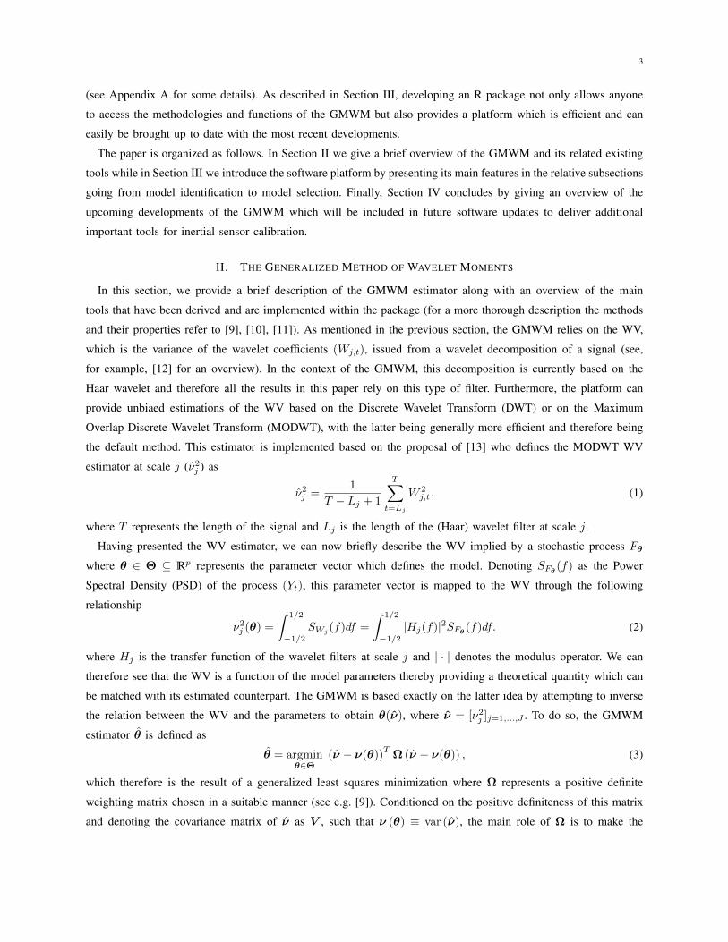
the object containing the estimated model. Additionally, one can seek to improve the fit by graphically observing

individual processes which contribute to the model by using the parameter “process.decomp = T”, which

gives Fig. 3b.

Aside from this graphical validation tool, the software provides rigorous statistical measures to assess the

significance of the estimated parameters and of the model as a whole. Supposing that the model has been saved

in an object called “gyro.y”, it is possible to obtain parameter confidence intervals (CIs) and a goodness-of-

fit test (see equation (4)) by using the function “summary(gyro.y, inference = T)”. The CIs provide a

measure of how accurate the parameters estimations are thereby giving information as to whether or not parameters

associated with a specific underlying process are significantly different from zero (e.g. H0 : θ = 0). Thus, this gives

a reasonable indication of whether a process should be kept in the model or not. However, with this being said, it is

known in the statistics literature that confidence intervals are conditional on the presence of other parameters in the

model. As a result, the main conclusion of whether a model is accurate should be obtained from the goodness-of-fit

test as it assesses how well the overall model explains the signal.

The tools provided by the new platform and described in this section are extremely important to understand

which models can be considered as good candidates to best describe the observed signal. The following step is to

select the “best” model(s) and the tools provided for this purpose are described in the next section.

10

10-9

10-8

10-7

10-6

10-5

10-2 10-1 100 101 102 103 104

Scale (s)

Wav

elet

Var

iance

(r

ad2/s

2)

Empirical WV

CI(,0.95)

Implied WV

Haar Wavelet Variance Classical Representation

1

(a) Comparison of observed WV (blue line) and model-implied WV

(orange line)

10-9

10-8

10-7

10-6

10-5

10-2 10-1 100 101 102 103 104

Scale (s)

Wav

elet

Vari

ance

(r

ad

2/s2

)

Empirical WV

CI(,0.95)

AR1

AR1

AR1

WN

QN

RW

Implied WV

Haar Wavelet Variance Classical Representation

2

(b) WV comparison with underlying process breakdown

Fig. 3: WV implied by the estimated 3*AR1()+WN()+QN()+RW() model compared to the empirical WV of the

NavChip Y-axis gyroscope.

C. Selecting the Model

The main goal of model selection is to identify the most appropriate model, among those that have been estimated,

to describe and predict future stochastic error measurements. Using the WIC, the two main options available to

rank the models according to this criterion are the following:

1) Manual: the function rank.models() allows to enter a set of candidate models from which the user

would like to select the best.

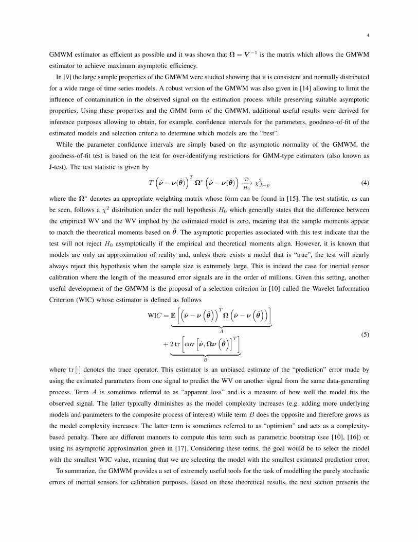
2) Automatic: the function auto.imu() allows to define an overall general model, sayMK , in which all K

candidate models are nested (e.g. Mk ⊆MK , for k = 1, . . . ,K). An example of this approach applied to

the mtig data is given in Fig. 4 where the implied WV of the selected models is compared to the observed

WV for each accelerometer and gyroscope.

Considering these two options, for both of them the platform also allows to choose the approach to estimate term

B in (5) as mentioned in Section II. The first option is given by the parametric bootstrap where H simulations are

performed on the kth candidate model Fθk to obtain estimates of ν(h) and ν(θ)(h)k that are then used to estimate the

“optimism” term. This option has been shown to possess good properties in various simulation studies and can be

used by specifying the parameter “bootstrap = T”. However, the latter is very demanding from a computational

standpoint while the asymptotic option, due to its closed analytical form, is less computationally intensive and has

some optimal theoretical properties as shown in [17]. Indeed, in terms of computational time, the asymptotic option

is roughly K times faster than the bootstrap option while at the same time being asymptotically loss efficient with

a null probability of underfitting.

In conclusion, given the features presented in this section and the previous ones, the challenge of correctly

estimating models for inertial sensor stochastic errors can more easily be met through this new platform. The latter

11

X Y Z

10-7

10-6

10-5

10-4

10-3

10-2

10-9

10-8

10-7

10-6

10-5

Accelerom

eterG

yroscop

e

10-1 100 101 102 103 10-1 100 101 102 103 10-1 100 101 102 103

Scale (s)

Wav

elet

Var

iance

(r

ad2/s

2)

Automatic Model Selection Results

5

Fig. 4: Results of running auto.imu() on the “mtig” data. Dashed line is the implied WV while the solid line

is the empirical WV.

not only easily estimates the complex error models which usually characterize IMUs but also delivers additional

tools to allow researchers to better understand these error models and to support their decisions for sensor calibration

purposes. As a support to the reader and potential user, an example of the code used to generate the results in the

previous sections can be found in Appendix D.

IV. UPCOMING FEATURES

The platform responds to the current needs for inertial sensor calibration while adding useful features which were

not available before. However, the idea of modelling latent processes which is behind the GMWM allows it to be

particularly suitable for extensions to more complicated settings. Different developments are indeed underway, or

close to completion, concerning issues which are extremely relevant for inertial sensor calibration. The following

sections briefly describe these extensions which will soon be implemented within the new software platform.

A. Multivariate GMWM

Currently sensor calibration is carried out separately for each accelerometer and gyroscope that build an IMU.

This procedure is valid if one supposes that the error signals of each of these components are independent from

each other which may not always be a realistic assumption to make. Using the latent process structure, the idea is to

explain the possible dependence of gyroscopes and accelerometers through a common model which is shared among

them. To provide an example, we could suppose that the error signals of the triad of gyroscopes (Y(x)t , Y

(y)t , Y

(z)t )

12

can be expressed as follows:Y

(x)t = Vt +W

(x)t

Y(y)t = Vt +W

(y)t

Y(z)t = Vt +W

(z)t

where Vt is the process which is shared between the gyroscopes and W (i)t is the specific process that characterizes

the error signal of the ith-axis gyroscope. The idea of expressing the model in this manner defines a new method for

the modelling of multivariate time series that is inspired by dynamic factor analysis. In this manner, we don’t only

explain the dependence between the sensor components but we also reduce the number of parameters to estimate

and obtain better fits. This feature will be added to the proposed platform once the theoretical properties of the

method are confirmed.

B. Calibration under dynamics

The correlation of IMU errors with system dynamics is a topic of great importance that may increase with the

spreading use of low-cost inertial sensors. Recent studies confirmed that system dynamics may have an important

influence on the characteristics of the error signal issued from inertial sensors (see [26]). The possibility of adapting

noise models according to the dynamics that the system is subject to should therefore be considered in the navigation

filters to enhance the performance of stochastic modeling. The proposed methodology is based on a non-stationary

adaptation of the GMWM framework. Let us consider the following example of a non-stationary AR1 process:

Yt = ρtYt−1 + εt, εtiid∼ (0, σ2

ε )

where ρt is the autoregressive parameter that now depends on the time t through a function m(·) : R 7→ (−1, 1).

Indeed, we define ρt = m(Zt−1β) where Zt−1 denotes a vector of dynamics and β is the parameter that explains

the impact of these dynamics on the parameters of the error signal model. This approach can be extended to other

parameters of typical error models considered for inertial sensor calibration. The properties of the WV estimator

ν and the implied WV ν(θ) considering such circumstances are being developed and will be later included in the

proposed platform.

C. Additional features

Other features are envisaged for the future updates of the package that are based on recently developed methods

and improvements on existing results. For example, it has been shown in [27] that adding further process moments

to the WV vector, such as the the mean or autocovariances, greatly improve the efficiency of the GMWM estimator.

This estimator is called the Augmented GMWM (GMWM+) and will be implemented as an additional option in

the gmwm.imu() function with the possibility of specifying the requirement on additional moments of the WV

vector. Furthermore, a test will be implemented to determine whether two error signals are generated from the same

model or not. Finally, additional features are planned such as the possibility to employ other kinds of wavelet filters

and use the robust WV as a basis for fault detection and isolation.

13

V. CONCLUSIONS

This paper presented the main features and function descriptions of the new software platform for inertial sensor

calibration based on the GMWM. This software is contained in an open-source R package called “gmwm” which

provides all the tools for the modelling of the complex stochastic error signals that characterize IMUs, although

this does not exclude the possibility of using it to estimate complex stochastic error models from other engineering

applications. As a statistically sound alternative to the AVLR and as a computationally efficient and numerically

stable alternative to the ML, the new platform based on C++ language allows to visualize data using the WV as

the main summary statistic in order to identify the possible models which can then be quickly and consistently

estimated. With graphical tools to assess how well the models fit the observed signals, the package also provides

functions to (automatically) select the best model(s) based on their estimated prediction error. These approaches

have been implemented in a computationally efficient manner and this paper has also provided details on how

these methods have been adapted to the specific and complex characteristics of IMU error signals through tailored

algorithms. All this allows to identify the model and estimate its parameters which can then be inserted into a

navigation filter (usually an extended Kalman filter) to improve the navigation accuracy of the sensors.

REFERENCES

[1] N. El-Sheimy and X. Niu, “The Promise of MEMS to the Navigation Community,” Inside GNSS, vol. 2, no. 2, pp. 46–56, 2007.

[2] O. J. Woodman, “An Introduction to Inertial Navigation,” University of Cambridge, Computer Laboratory, Tech. Rep. UCAMCL-TR-696,

vol. 14, p. 15, 2007.

[3] Y. Stebler, S. Guerrier, J. Skaloud, and M.-P. Victoria-Feser, “Constrained Expectation-Maximization Algorithm for Stochastic Inertial

Error Modeling: Study of Feasibility,” Measurement Science and Technology, vol. 22, no. 8, pp. 1–12, 2011.

[4] Y. Zaho, M. Horemuz, and L. E. Sjoberg, “Stochastic Modelling and Analysis of IMU Sensor Errors,” Archives of Photogrammetry,

Cartography and Remote Sensing, vol. 22, pp. 437–449, 2011.

[5] J. Nikolic, P. Furgale, A. Melzer, and R. Siegwart, “Maximum Likelihood Identification of Inertial Sensor Noise Model Parameters,”

Sensors Journal, IEEE, vol. 16, no. 1, pp. 163–176, 2016.

[6] N. El-Sheimy, H. Hou, and X. Niu, “Analysis and Modeling of Inertial Sensors using Allan Variance,” IEEE Transactions on

Instrumentation and Measurement, vol. 57, no. 1, pp. 140–149, January 2008.

[7] Guerrier, S. and Molinari, R. and Stebler, Y., “Theoretical Limitations of Allan Variance-based Regression for Time Series Model

Estimation,” IEEE Signal Processing Letters (to appear), pp. 1–10, 2016.

[8] R. J. Vaccaro and A. S. Zaki, “Statistical Modeling of Rate Gyros,” IEEE Transactions on Instrumentation and Measurement, vol. 61,

no. 3, pp. 673–684, 2012.

[9] S. Guerrier, J. Skaloud, Y. Stebler, and M.-P. Victoria-Feser, “Wavelet Variance based Estimation for Composite Stochastic Processes,”

Journal of the American Statistical Association, vol. 108, no. 503, pp. 1021–1030, 2013.

[10] S. Guerrier, R. Molinari, and J. Skaloud, “Automatic Identification and Calibration of Stochastic Parameters in Inertial Sensors,” Navigation,

vol. 62, no. 4, pp. 265–272, 2015.

[11] S. Guerrier and R. Molinari, “Robust Inference for Time Series Models: a Wavelet-based Framework,” Submitted Manuscript, pp. 1–62,

2015.

[12] D. B. Percival and A. T. Walden, Wavelet Methods for Time Series Analysis. Cambridge University Press, 2000.

[13] D. B. Percival, “On Estimation of the Wavelet Variance,” Biometrika, vol. 82, pp. 619–631, 1995.

[14] S. Guerrier and R. Molinari, “Fast and robust parametric estimation for time series and spatial models,” Submitted manuscript, 2016.

14

[15] L. P. Hansen, “Large Sample Properties of Generalized Method of Moments Estimators,” Econometrica: Journal of the Econometric

Society, pp. 1029–1054, 1982.

[16] B. Efron, “The Estimation of Prediction Error,” Journal of the American Statistical Association, vol. 99, no. 467, pp. 619–632, 2004.

[17] Zhang, X. and Guerrier, S., “Covariance Penalty Based Model Selection Criterion for Indirect Estimators,” Submitted Working Paper, pp.

1–30, 2015.

[18] R. C. Team, R: A Language and Environment for Statistical Computing, R Foundation for Statistical Computing, Vienna, Austria, 2014.

[Online]. Available: http://www.R-project.org

[19] D. Eddelbuettel, R. Francois, J. Allaire, J. Chambers, D. Bates, and K. Ushey, “Rcpp: Seamless R and C++ integration,” Journal of

Statistical Software, vol. 40, no. 8, pp. 1–18, 2011.

[20] D. Eddelbuettel and C. Sanderson, “RcppArmadillo: Accelerating R with High-Performance C++ Linear Algebra,” Computational Statistics

& Data Analysis, vol. 71, pp. 1054–1063, 2014.

[21] C. Sanderson, Armadillo: An Open Source C++ Linear Algebra Library for Fast Prototyping and Computationally Intensive Experiments,

2010.

[22] Y. Stebler, S. Guerrier, J. Skaloud, and M.-P. Victoria-Feser, Generalized Method of Wavelet Moments (GMWM) Modelling Software,

1st ed., EPFL, CH-1015 Lausanne, Switzerland, 2012.

[23] W. Riley, Handbook of Frequency. NIST, 2008.

[24] S. Guerrier, R. Molinari, J. Skaloud, and M.-P. Victoria-Feser, “An Algorithm for Automatic Inertial Sensors Calibration,” in ION GNSS,

2013.

[25] D. Mondal and D. B. Percival, “M-Estimation of Wavelet Variance,” Annals of the Institute of Statistical Mathematics, vol. 64, no. 1, pp.

27–53, 2012.

[26] Y. Stebler, S. Guerrier, J. Skaloud, R. Molinari, and M. P. Victoria-Feser, “Study of MEMS-based Inertial Sensors Operating in Dynamic

Conditions,” in Position, Location and Navigation Symposium - PLANS 2014, 2014 IEEE/ION, 2014, pp. 1227–1231.

[27] S. Guerrier, R. Molinari, and Y. Stebler, “Wavelet-based Improvements for Inertial Sensor Error Modelling,” Submitted working paper,

2016.

[28] W. Kusnierczyk, rbenchmark: Benchmarking Routine for R, 2012, R package version 1.0.0.

[29] Y. Stebler, S. Guerrier, J. Skaloud, and M. P. Victoria-Feser, “Generalized Method of Wavelet Moments for Inertial Navigation Filter

Design,” IEEE Transactions on Aerospace and Electronic Systems, vol. 50, no. 3, pp. 2269–2283, 2014.

15

APPENDIX A

BENCHMARKS

One of the driving design principles behind the proposed platform is its computational efficiency. To achieve this

goal, the computational backend is written completely in C++ using the Armadillo matrix library (see [21]). The

implementation of each function is highly efficient due to the manner in which they are implemented. Specifically,

multiple functions for the same task were created within C++ and then benchmarked. The benchmarking was

conducted using the “rbenchmark” package [28] with each function being called 100 times. The function that used

the least amount of time among the C++ implementations was then included within the package. This bottom-up

approach used to create the package not only delivers a very efficient implementation of the GMWM estimator

but also of different wavelet-based methods and random process generation. To illustrate, we provide details on

the overall computational time across a wide range of sample sizes to estimate a 3*GM() model under both

the standard and robust settings in two different modes: user-supplied and guessed parameters. The user-supplied

parameters were taken to be the exact parameters whereas the guessed parameters relied on the initial starting

algorithm described in Appendix C. The latter algorithm was based on a range of initial guesses going from 100

to 1,000,000. The time reported in Tab. II and III is by the number of seconds required to estimate the model.

Type 100 1,000 10,000 100,000 1,000,000

Exact Values 0.0100 0.0188 0.0300 0.1408 1.5473

Guessed 1,000 0.0342 0.0369 0.0594 0.1714 1.5965

Guessed 10,000 0.0755 0.0794 0.1250 0.2511 1.6647

Guessed 20,000 0.1216 0.1386 0.2005 0.3411 1.7917

Tab. II: Standard estimation of a 3*GM() model using “gmwm.imu()” in seconds

Type 1,000 10,000 100,000 1,000,000

Exact Values 0.0327 0.0816 0.6839 11.4097

Guessed 1,000 0.0546 0.1081 0.6875 11.4575

Guessed 10,000 0.1135 0.1791 0.7687 11.5385

Guessed 20,000 0.1666 0.2516 0.8556 11.5957

Tab. III: Robust estimation of a 3*GM() model using “gmwm.imu()” in seconds

APPENDIX B

HOW TO IMPORT IMU DATA

The first step towards the modelling of the inertial sensor stochastic error is loading the data onto the platform.

This is done by:

16

1) Loading data in .txt or .csv format;

2) Reading in IMU binary files.

In the first case, the user must also cast the data as an “imu” object whereas this is automatically done when

loading the data in the second case. Below is an example that displays each of these cases.

# Case 1a: Reads in data that is separated by tab

ds = read.table("path/to/file.txt")

# Case 1b: Reads in data that is separated by comma

ds = read.csv("path/to/file.csv")

# Case 2: Cast data loaded into R to IMU object-type

# for use in the gmwm routines

sensors = imu(ds, accelerometer = 1:3, gyroscope = 1:3,

freq = 100)

# Case 3: Read an imu binary file and cast object as

# an IMU-type

sensors = read.imu("˜/path/to/file.imu", "IMU_TYPE")

The binary file reader currently supports the binary record format used by well known commercial software

such as Applanix (PosProc) and Novatel/Waypoint (IExplorer). This format is aptly described as a seven column

layout where the first column of the data contains time data, columns 2-4 contain gyroscope values and columns

5-7 contain accelerometer values for axes X, Y, and Z. Upon loading, appropriate scaling factors are applied to the

data. As a result, the following types of IMU can be loaded via their binary: IMAR, LN200, LN200IG, IXSEA,

NAVCHIP INT and NAVCHIP FLT. For more details, please see the read.imu() help documentation.

APPENDIX C

OPTIMIZATION STARTING VALUES ALGORITHM

To start any optimization procedure starting values are needed and this is the case also for the GMWM procedure

with the optimization in (3). The platform uses an algorithm to find appropriate starting values and this is described

in three parts below: a general overview of the algorithm (Algorithm 1), a heuristic approach to determining the

dominating process (Algorithm 2), and a focus on a specific step based on the required processes to be estimated

(Algorithm 3).

17

Inputs : An empty parameter vector θ that defines the model, the wavelet variance for the first two scales,

and the slope of the data(

min(x)−max(x)length (x)

).

Output: Starting values to estimate the parameter vector θ

Step 1: Compute the total variance σ2T = var ν for all scales obtained with Equation 1.

Step 2: Determine the process that dominates the initial scales using Algorithm 2.

Step 3a: Randomly sample G times from the parameter spaces depending on the type of process. At the start

of each new round of guessing for all parameters, use the domination result from Step 2 to select the starting

condition of the “GM” / “AR1” process:

if QN dominates thenDraw R ∼ U [0, 1]

if R ≤ 0.75 thenStart AR1 or GM on condition 2 in Algorithm 3

else if WN dominates thenStart AR1 or GM on condition 2 in Algorithm 3

Step 3b: See Algorithm 3 for details on parameter selection for each process.

Step 4: Select the starting parameter vector θ(0) with the smallest objective function value given by the

flattening algorithm described in [29]:

θ(0) = arg minθ∈Θ

(1− ν (θ)

ν

)T (1− ν (θ)

ν

)(6)

Algorithm 1: Starting Values Algorithm

Inputs : Process’ wavelet variance, and the slope of the data(

min(x)−max(x)length (x)

).

Output: Process that dominates the initial scales.

Step 2a: Compute the slope, s, between the first wavelet variance, ν1, and the upper and lower confidence

bounds of the second, a =[

ην2χ2η(0.975)

, ην2χ2η(0.025)

], using s = log(a)−log(ν1)

log(4) , where

η = max((N − Lj + 1) /2j , 1

)Step 2b: Determine whether QN, WN, or AR1/GM dominates the initial scales based on a slope heuristic:

if max (s) < −.5 thenQN Dominates

else if min (s) > −.5 thenAR1/GM Dominates

elseWN Dominates

Algorithm 2: Process Domination Algorithm

18

Inputs : An empty parameter vector θ that defines the model, the process’ wavelet variance, and the slope of

the data.

Output: A parametric model Fθ

Step 3b: Select the appropriate realization generator based on process type

if AR1 or GM then

if AR/GM on condition 1 thenDraw U ∼ U (0, 1/3) for φ = 1−

√1−3U5

Draw σ2 ∼ U(σ2T (1−φ)2

2 , σ2T (1− φ)

2)

else if AR/GM on condition 2 thenDraw φi ∼ U (max (0.9, φi−1) , 0.999995)

Draw σ2 ∼ U(

0,σ2T (1−φ2

i )100

)else

Draw U ∼ U (0, 1/3) for φi = (.999995− φi−1)(√

1− 3U)

+ φi−1

Draw σ2 ∼ U(σ2T (1−φ)2

2 , σ2T (1− φ)

2)

Increase the condition by 1.

else if DR thenCalculate the slope of the data: R = max(x)−min(x)

length(x)

Draw ω ∼ U(R

100 ,R2

)else if RW then

Draw γ2 ∼ U(

σ2T

105·N ,σ2T

N

)else if WN then

if WN Dominates then

Draw σ2 ∼ U(σ2T

2 , σ2T

)else

Draw σ2 ∼ U(σ2T

105 ,σ2T

10

)else

if QN Dominates then

Draw Q2 ∼ U(σ2T

8 ,σ2T

3

)else

Draw Q2 ∼ U(

σ2T

2·105 ,σ2T

100

)

Algorithm 3: Process-specific Starting Values Algorithm

19

APPENDIX D

CODE USED IN PAPER

The following code was used to generate some of the results and figures included in the paper and provides

insight to the use of the “gmwm” platform. Please note that the following code was executed under version 3.0.0

of both the “gmwm” and “imudata” R package.

# 0. Preparing the workspace

# Load R Package

library("gmwm")

# Load in MTIG data. If the data package is not installed,

# then install it.

if(!require("imudata"))

install_imudata()

library("imudata")

# Read in Binary IMU Data

navchip = read.imu("˜/IMU_data/navchip_4h.imu","NAVCHIP_FLT")

# 1. WAV-AR All Navchip

# Obtain the wavelet variance of all sensors

# in imu object.

wv.navchip = wvar(navchip)

# Plot the Wavelet Variance of each sensor

plot(wv.navchip)

# 2. Generate models for each sensor

navchip.gx = gmwm.imu(2*GM() + WN() + DR() + QN() + RW(),

navchip[,1])

navchip.gy = gmwm.imu(3*GM() + WN() + QN() + RW(),

navchip[,2])

navchip.gz = gmwm.imu(2*GM() + WN() + DR() + QN() + RW(),

navchip[,3])

navchip.ax = gmwm.imu(4*GM() + QN() + RW(), navchip[,4])

navchip.ay = gmwm.imu(4*GM() + QN() + RW(), navchip[,5])

navchip.az = gmwm.imu(3*GM() + QN(), navchip[,6])

# Robust model generation

navchip.gy.r = gmwm.imu(3*GM() + WN() + QN() + RW(),

navchip[,2], robust = T)

# Summary statistics

sm.navchip.gy = summary(navchip.gy, inference = T)

sm.navchip.gy.r = summary(navchip.gy.r, inference = T)

20

# 3. Compare Classical with Robust WV

compare.wvar(navchip.gy, navchip.gy.r)

# 4. Load and cast data for MTiG

data("imu6")

# Cast as an IMU

sensors = imu(imu6, gyros = 1:3, accels = 4:6, freq = 100)

# 5. Obtain WV and plot WV

wv.sensors = wvar(sensors)

plot(wv.sensors)

# 6. Automatic Model Selection with Overall Model Guess

models.sensors = auto.imu(sensors,

model = 4 * AR1() + WN() + RW())

# 7. Visually see the best models

plot(models.sensors)