1

A Dual Camera System for High SpatiotemporalResolution Video Acquisition

Ming Cheng, Zhan Ma, M. Salman Asif, Yiling Xu, Haojie Liu, Wenbo Bao, and Jun Sun

Abstract—This paper presents a dual camera system for high spatiotemporal resolution (HSTR) video acquisition, where one camerashoots a video with high spatial resolution and low frame rate (HSR-LFR) and another one captures a low spatial resolution and highframe rate (LSR-HFR) video. Our main goal is to combine videos from LSR-HFR and HSR-LFR cameras to create an HSTR video. Wepropose an end-to-end learning framework, AWnet, mainly consisting of a FlowNet and a FusionNet that learn an adaptive weightingfunction in pixel domain to combine inputs in a frame recurrent fashion. To improve the reconstruction quality for cameras used inreality, we also introduce noise regularization under the same framework. Our method has demonstrated noticeable performance gainsin terms of both objective PSNR measurement in simulation with different publicly available video and light-field datasets and subjectiveevaluation with real data captured by dual iPhone 7 and Grasshopper3 cameras. Ablation studies are further conducted to investigateand explore various aspects (such as reference structure, camera parallax, exposure time, etc) of our system to fully understand itscapability for potential applications.

Index Terms—Dual camera system, high spatiotemporal resolution, super-resolution, optical flow, spatial information, end-to-endlearning

F

1 INTRODUCTION

High-speed cameras play an important role in various modernimaging and photography tasks including sports photography, filmspecial effects, scientific research, and industrial monitoring. Theyallow us to see very fast phenomena that are easily overlooked andcan not be captured at ordinary speed, such as a droplet, full-speedfan rotation, or even a gun fire. These cameras can capture videosat high frame-rates that range from several hundred to severalthousand frames per second (FPS), while an ordinary cameraoperates at 30 to 60 FPS. The high frame-rates often come at theexpense of spatial resolution; especially, consumer-level camerasthat sacrifice the spatial resolution to maintain the high framerate acquisition. For example, popular iPhone 7 can capture 4Kvideos at 30 FPS, but can only offer 720p resolution at 240 FPSbecause of the limitation of the data I/O throughput. Some special-purpose and professional high-speed cameras can capture highspatiotemporal resolution (HSTR) videos, but they are typicallyvery expensive (e.g., Phantom Flex4K1 with price starting at$110K) and beyond the budget of a majority of consumers.

A naıve solution to obtain a HSTR video from a video withhigh spatial resolution and low frame rate (HSR-LFR) or lowspatial resolution and high frame rate (LSR-HFR) is to upsamplealong temporal or spatial direction, respectively. Upsampling intemporal resolution or frame rate upconversion of an HSR-LFR

M. Cheng, Z. Ma and H. Liu are with Nanjing University, Nanjing, Jiangsu,China. M. S. Asif is with the University of California at Riverside. M. Cheng isalso with Shanghai JiaoTong University, Shanghai, China. Y. Xu, W. Bao andJ. Sun are with Shanghai JiaoTong University, Shanghai, China. Z. Ma is thecorresponding author of this paper. M. S. Asif and Y. Xu are co-correspondingauthors of this paper.This paper is supported in part by National Natural Science Foundation ofChina (61971282), National Key Research and Development Project of ChinaScience and Technology Exchange Center (2018YFE0206700) and ScientificResearch Plan of the Science and Technology Commission of ShanghaiMunicipality (18511105402).

1. https://www.phantomhighspeed.com/products/cameras/4kmedia/flex4k

(b) LSR‐HFR 

(C) HSTR 

HSR‐LFR camera LSR‐HFR camera

(a) HSR‐LFR

FlowNetUpScale

FusionNet

AWnet

Warp Flow

Fig. 1. Snapshots of high spatial resolution-low frame rate (HSR-LFR) and low spatial resolution-high frame rate (LSR-HFR) videos andsynthesized high spatiotemporal resolution (HSTR) video. A womanis throwing a ping-pong ball in indoor space. (a) HSR-LFR video4K@30FPS frame with zoomed-in region showing motion blur; (b) LSR-HFR video 720p@240FPS frame with zoomed-region showing spatialblur; (c) HSTR video 4K@240FPS frame.

arX

iv:1

909.

1305

1v2

[ee

ss.I

V]

24

Mar

202

0

2

video (e.g., 4K at 30FPS) involves imputing missing framesby interpolating motion between the observed frames, whichis challenging because of the motion blur introduced by longexposure and inaccuracies in motion representation under thecommonly-used uniform translational motion assumption [47].On the other hand, upsampling spatial resolution of a LSR-HFRvideo can be performed using a variety of existing super-resolutionmethodologies [33], [51], but they often provide smoothed imagesin which high frequency spatial details of the captured sceneare missing. Figure 1 highlights these effects, where HSR-LFR(4K at 30FPS) video contains motion blur in the regions of fastmotion and LSR-HFR (720p at 240FPS) has a uniform spatial blurbecause of limited spatial resolution.

In this paper, we propose a dual camera system for HSTRvideo YHSTR(t) acquisition, as shown in Fig. 1, where one cameracaptures a HSR-LFR video XHSR−LFR(t) with rich spatial infor-mation (i.e., sharp spatial details for textures and edges), andthe other one records a HFR-LSR video xLSR−HFR(t) with fine-grain temporal information (i.e., intricate motion flows). We thenfuse these two videos via a learning-based approach to produce afinal HSTR video with both appealing spatial details and accuratemotion. In another words, we aim to transfer the rich spatial detailsfrom HSR-LFR frame to the associated LSR-HFR frames whileretaining accurate motion in the entire sequence.

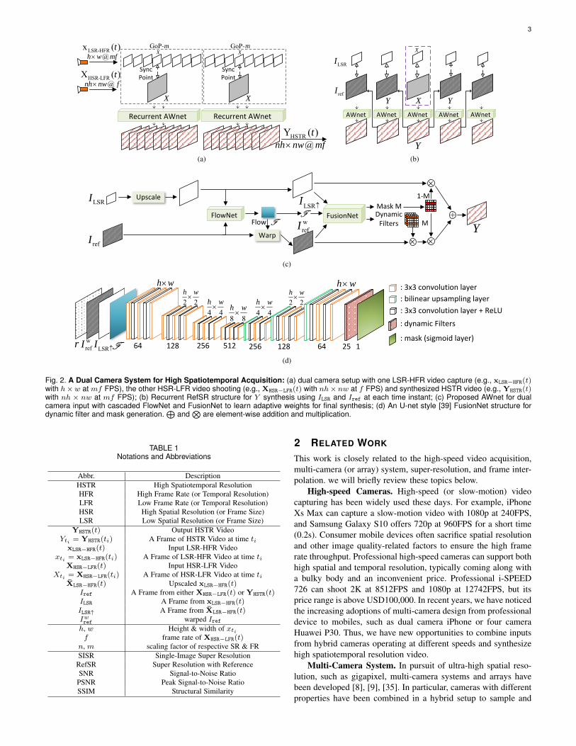
Our method performs spatiotemporal super-resolution in aframe recurrent manner within a synchronized GoP (group ofpictures) to exploit the spatial-temporal priors in Fig. 2(a). Adetailed block diagram of our proposed method is shown inFig. 2(b). The synthesis process has two main parts: FlowNetand FusionNet, which are placed consecutively in Fig. 2(c). ILSRdenotes a frame captured with LSR-HFR camera. The FlowNetaccepts an upsampled LSR-HFR image (ILSR↑) and a referenceimage (Iref) to provide the optical flow (denoted as F ) and awarped reference image (Iwref). The reference image can eitherbe a frame from the HSR-LFR camera at a synchronized timeinstant or a synthesized frame Y . Our dual camera based systemcan be viewed as a method in the class of ”super-resolution withreference” (RefSR) methods [7], [51]. The FusionNet accepts theoptical flow, upsampled LSR-HFR image, and warped referenceimage, and learns dynamic filters and masking pattern that areused to adaptively weigh the contribution of ILSR and Iref fora high-quality reconstruction Y . We use PWC-Net [42] as ourFlowNet and a U-net as our FusionNet [39]. More details aboutnetwork architecture are provided in Section 3 and in Fig. 2(d).Our method learns adaptive weights to combine the hybrid inputs,therefore, we refer to it as an adaptive weighting network (AWnet).

Our proposed AWnet is trained using Vimeo90K dataset. Wefirst evaluate the performance of our method using simulationson publicly available datasets. Then we measure the performanceof our method on videos captured with our custom dual-cameraprototype. In our experimental evaluations, we observe that thequality of HSTR video degrades when we directly use modelstrained with Vimeo90K training images. One reason for theperformance degradation is the presence of large sensor noise inILSR when LSR-HFR video is captured with short exposure time(especially under low light conditions). Vimeo90K training data isvirtually free of noise and other nonidealities that a real data cap-ture encounters. To make our system robust to noise, we introducenoise at various levels in original Vimeo90K training data whenperforming the end-to-end learning. Such noise regularization canintelligently shift weights between ILSR and Iref, offering much

better reconstruction quality, under the same framework.Extensive simulations are conducted using both simulation

data from publicly accessible videos, dual-camera captures,and light field datasets (such as Vimeo90K [47], KITTI [36],Flower [41], LFVideo [43] and Stanford Light Field [1] datasets2),and real data (captured with custom-built dual iPhone 7 orGrasshopper3 cameras). Our proposed AWnet demonstrates no-ticeable performance gains over the existing super-resolution andframe interpolation methods, in objective and subjective measures.In our tests with simulations using Vimeo90K testing samples,our proposed model offers ∼ 0.7 dB PSNR gain compared to thestate-of-the-art CrossNet [51] and ∼ 6 dB PSNR compared to thepopular single-image super-resolution (SISR) method EDSR [33].Our proposed AWnet provides the best performance on other videoand lightfield datasets. In our tests with real data, we observeperceptual enhancements for various scenarios with indoor andoutdoor activities under different lighting conditions.

We also offer ablation studies to fully understand the capabilityof our dual camera AWnet system, by analyzing various aspectsin practice, such as the impacts of upscaling filters, referencestructure, camera parallaxes, exposure time, etc. All these testsdemonstrate the efficiency of our dual camera system for super-resolution and frame interpolation, to maintain sharp spatial detailsand accurate temporal motions jointly, leading to the state-of-the-art performance.

Main contributions of this work are highlighted below.• A practical system for high spatiotemporal video acquisition

uses a dual off-the-shelf camera setup. Videos from two cam-eras, operating at different spatial and temporal resolution,are combined using an end-to-end learning-based adaptiveweighting to preserve spatial and temporal information inboth inputs for a high-quality reconstruction.

• Cascaded FlowNet and FusionNet are applied to learn em-bedded spatial and temporal features for adaptive weightsderivation in a frame recurrent way. These weights can beregularized using added noise to efficiently handle noiseand other nonidealities in real data captured with consumercameras.

• Our dual camera AWnet system demonstrates the state-of-the-art performance for super-resolution and frame interpo-lation, using both simulation data from public and real datacaptured by cameras.

• We analyze the robustness and efficiency of our systemthrough a series of ablation studies to explore the impactsof upscaling filters, reference structure, camera parallaxes,exposure time, etc, which promises generalization in a varietyof practical scenarios.

The remainder of this paper is structured as follows. Section 2provides a brief overview of related work in literature, includingsystem prototypes and applications. Section 3 details our proposedsystem and associated learning algorithms, followed by trainingprocessing in Section 4. The experimental results on simulationdata and real data captured by cameras are shown in Section 5.We further break down our system to analyze and study itsvarious aspects, such as the camera parallax, scaling filters, etc,in Section 6. Finally, conclusion is drawn in Section 7. Table 1contains a list of all the notions and acronyms used throughoutthis paper.

2. Note that these datasets are widely used in literature for performancebenchmark [51].

3

GoP-m GoP-m

Sync Point

X X

X X

@nh nw fHSR-LFRX ( )t

LSR-HFRx ( )t@h w mf

Sync Point

Recurrent AWnet Recurrent AWnet

@nh nw mfHSTRY ( )t

(a)

X

XY Y

Y

LSRI

refI

AWnetAWnetAWnetAWnetAWnet

(b)

LSRI

refI

Upscale

Warp

LSRI

wrefIF Dynamic 

Filters

Mask M

1‐M

MY

FFlowFlowNet FusionNet

+

(c)

: dynamic Filters

: mask (sigmoid layer)64 128 256 512 256 128 64

: 3x3 convolution layer

: bilinear upsampling layer

25 1FLSRI

wrefI

: 3x3 convolution layer + ReLU

r

h w

2 2

h w

4 4

h w

8 8

h w

2 2

h w

4 4

h w

h w

(d)

Fig. 2. A Dual Camera System for High Spatiotemporal Acquisition: (a) dual camera setup with one LSR-HFR video capture (e.g., xLSR−HFR(t)with h×w at mf FPS), the other HSR-LFR video shooting (e.g., XHSR−LFR(t) with nh× nw at f FPS) and synthesized HSTR video (e.g., YHSTR(t)with nh × nw at mf FPS); (b) Recurrent RefSR structure for Y synthesis using ILSR and Iref at each time instant; (c) Proposed AWnet for dualcamera input with cascaded FlowNet and FusionNet to learn adaptive weights for final synthesis; (d) An U-net style [39] FusionNet structure fordynamic filter and mask generation.

⊕and

⊗are element-wise addition and multiplication.

TABLE 1Notations and Abbreviations

Abbr. DescriptionHSTR High Spatiotemporal ResolutionHFR High Frame Rate (or Temporal Resolution)LFR Low Frame Rate (or Temporal Resolution)HSR High Spatial Resolution (or Frame Size)LSR Low Spatial Resolution (or Frame Size)

YHSTR(t) Output HSTR VideoYti = YHSTR(ti) A Frame of HSTR Video at time ti

xLSR−HFR(t) Input LSR-HFR Videoxti = xLSR−HFR(ti) A Frame of LSR-HFR Video at time ti

XHSR−LFR(t) Input HSR-LFR VideoXti = XHSR−LFR(ti) A Frame of HSR-LFR Video at time ti

XLSR−HFR(t) Upscaled xLSR−HFR(t)Iref A Frame from either XHSR−LFR(t) or YHSTR(t)ILSR A Frame from xLSR−HFR(t)ILSR↑ A Frame from XLSR−HFR(t)Iwref warped Irefh, w Height & width of xtif frame rate of XHSR−LFR(t)

n, m scaling factor of respective SR & FRSISR Single-Image Super Resolution

RefSR Super Resolution with ReferenceSNR Signal-to-Noise Ratio

PSNR Peak Signal-to-Noise RatioSSIM Structural Similarity

2 RELATED WORK

This work is closely related to the high-speed video acquisition,multi-camera (or array) system, super-resolution, and frame inter-polation. we will briefly review these topics below.

High-speed Cameras. High-speed (or slow-motion) videocapturing has been widely used these days. For example, iPhoneXs Max can capture a slow-motion video with 1080p at 240FPS,and Samsung Galaxy S10 offers 720p at 960FPS for a short time(0.2s). Consumer mobile devices often sacrifice spatial resolutionand other image quality-related factors to ensure the high framerate throughput. Professional high-speed cameras can support bothhigh spatial and temporal resolution, typically coming along witha bulky body and an inconvenient price. Professional i-SPEED726 can shoot 2K at 8512FPS and 1080p at 12742FPS, but itsprice range is above USD100,000. In recent years, we have noticedthe increasing adoptions of multi-camera design from professionaldevice to mobiles, such as dual camera iPhone or four cameraHuawei P30. Thus, we have new opportunities to combine inputsfrom hybrid cameras operating at different speeds and synthesizehigh spatiotemporal resolution video.

Multi-Camera System. In pursuit of ultra-high spatial reso-lution, such as gigapixel, multi-camera systems and arrays havebeen developed [8], [9], [35]. In particular, cameras with differentproperties have been combined in a hybrid setup to sample and

4

synthesize images from a variety of light components, such ashyperspectral imaging [12], low light imaging [32], and lightfields [45], [51]. Pelican imaging and Light are two recent com-panies that launched products with multiple cameras on boardcapturing a diverse set of images and synthesizing a desired imagewith high dynamic range, long-range depth, or light field [45] .The hybrid camera or multi-camera systems have also been usedto combine different imaging sources to perform super-resolutionand frame interpolation (for frame rate up-conversion) [51]. Ourproposed work also belongs to the hybrid camera setup thatcaptures two video streams, one at HSR-LFR and the other one atLSR-HFR, and combine them to synthesize a final HSTR video.

Super-Resolution. Single image super resolution (SISR)methods upscale individual images, which include traditionalmethods based on bilinear and bicubic filters and recently-introduced learning-based techniques [31], [33]. SISR methodscan be easily extended to support video or multi-frame super-resolution [11], [27], [40]. In the case of multi-camera setup,super-resolution can be performed using some source as a ref-erence [7], [17]. Low resolution images/videos can be upscaledwith references (e.g., RefSR) from other viewpoints, leadingto significant quality improvement [7], [49]–[51]. Such RefSRapproaches have also been widely used in lightfield imaging [7],[51].

Frame Interpolation. Linear translation motion is a con-ventional assumption that has been extensively used in differentinterpolation-based methods to impute missing frames for framerate up-conversion. Motion estimation can be performed usingclassical block-based or dense optical flow-based methods [2]–[5], [25], [37], [47]. Classical optimization-based and modernlearning-based methods mainly try to retain smooth motion alongthe temporal trajectory while resolving occlusion-induced arti-facts. Accurate motion flow estimation remains a challenging taskbecause of the inconsistent object movements and motion-inducedocclusion. As we discussed below, this issue can be significantlyalleviated with the help of a high frame-rate video as a reference.

3 DUAL CAMERA SYSTEM FOR HIGH SPATIOTEM-PORAL RESOLUTION VIDEO

We propose a dual camera system for HSTR video acquisition,as illustrated in Fig. 2. One camera records a HSR-LFR videoXHSR−LFR(t) with nh×nw at f FPS, while the other one capturesa LSR-HFR video xLSR−HFR(t) with h×w atmf FPS. We learn anadaptive model to weigh contributions from the two input videosand synthesize a final HSTR output video YHSTR(t) with nh×nwat mf FPS. We use integer multipliers, m and n, for simplicityin this work, but different multipliers can be easily used. Insubsequent sections, we first offer experimental observations that asingle camera setup could not provide high-quality reconstructionof HSTR video via naıve spatial super-revolution or temporalframe interpolation. Then we discuss our dual camera systemand algorithm development. Note that even though we particularlyemphasize current work in a dual camera setup, this work can begeneralized to other multi-camera configurations since the RefSRstructure can be flexibly extended.

3.1 Single Camera System

Let us consider the following model for an image frame capturedat time instance t of a camera as

I(t) =

∫ t

t−TS(τ)dτ + n(t), (1)

where S(τ) is the instantaneous photon density reflected fromthe physical scene, T denotes the exposure time, and n(t) isthe noise accumulated in the camera during a single exposureand the subsequent readout process. In other words, image isrepresented as the accumulated photons during the exposure time(according to the shutter speed). A typical consumer camera usedin mobile devices3 usually automatically adjusts the aperture size,ISO settings, and shutter speed according to a specific “shootingmode”. Thus, exposure time duration T is uncertain and changesaccording to the scene content.

For example, normal video capture in iPhone 7 offers HSR(e.g., 4K) at f = 30FPS (i.e., HSR-LFR video), leading to richspatial details but blurred motion. On the other hand, the slow-motion mode provides LSR (e.g., < 720p) at mf = 240FPS(LSR-HFR video), resulting in accurate motion acquisition atthe expense of spatial information, dynamic range, and SNR.Figure 1 shows two snapshots for respective HSR-LFR and LSR-HFR videos. As we can see, the spatial quality of the LSR-HFRframe is poor because some spatial information is missing in theslow-motion mode. Similarly, motion blur is clearly observed forthe HSR-LFR frame because of insufficient temporal sampling.

Our experimental results in Tables 2, 3 and Figs. 6, 7, 8 showthat frame-by-frame super-resolution or temporal interpolation offrames from a single camera could not provide the same qualityas the dual camera setup, both objectively and subjectively.

These observations suggest that we are not capable of recon-structing high-quality HSTR video by applying spatial interpola-tion on the LSR-HFR video or temporal interpolation on HSR-LFR video. Therefore, we propose to use a dual camera system inwhich the main problem is to synthesize two input videos whilepreserving the sharp spatial details from the HSR-LFR video andreal motions from the LSR-HFR video.

3.2 Dual Camera System

For a dual camera system setup, given a LSR-HFR videoxLSR−HFR(t) recorded at mf FPS and an additional HSR-LFRvideo XHSR−LFR(t) recorded at f FPS from another view, wewish to generate a final HSTR video YHSTR(t) at mf FPS. Torecover high-quality HSTR video, we seek to preserve the realmotion field from the LSR-HFR camera input and the detailedspatial information from the HSR-LSR input. To do that, weneed to design an effective mechanism to extract, transfer, andfuse appropriate information or features intelligently from the twoinputs.

Dual cameras are configured and synchronized with a certainbaseline distance to capture the instantaneous frames of the samescene. Because of the different frame rates for the respective HSR-LFR and LSR-HFR cameras, the exposure time of the HSR-LFR frame are often much longer than the LSR-HFR frames,especially in the low-light settings. Based on the imaging model

3. We use mobile phone camera as an example for its massive marketadoption.

5

in (1), we can also consider the HSR-LFR frame as the high-spatial-resolution version of the summation of associated LSR-HFR frames, which will model the motion blur.

We divide the entire processing into two major steps: (1)optical flow estimation to compensate for motion and parallaxes tofacilitate image fusion; (2) fusion processing to compute appropri-ate weighting functions (e.g., dynamic filter and mask in our work)through extensive feature learning. We propose to apply learnednetworks to perform aforementioned temporal and spatial featureextraction, transfer, and fusion. For convenience, we note them as“FlowNet” and “FusionNet” respectively, shown in Fig. 2(c).

We will synthesize the HSTR video in batches of group-of-pictures (GoP), as shown in Fig. 2(a). Because the same processingpattern is applied in each GoP, we will explain the specific stepsfor a single GoP. A GoP is a set of frames from the LSR-HFRvideo that are aligned to a specific time stamp of the HSR-LFRvideo. Since we assume that the LSR-HFR video is recorded atmf FPS and the HSR-LFR at f FPS, we find it convenient touse a GoP with m frames that we call GoP-m in the remainderof this paper. A GoP-m consists of m LSR-HFR frames that arealigned with one HSR-LFR frame. In particular, we assume thatthe HSR-LFR frame timestamp is in the middle of the timestampsfor all the LSR-HFR frames in a GoP-m. For instance, a GoP-mthat contains LSR-HFR frames at times [t− k′∆t, . . . , t+ k∆t]are synchronized with HSR-LFR frame at t, where k′ = dm2 e−1,k = bm2 c, and ∆t is the time interval between two adjacent HSR-LFR frames. To maximize the use of spatial information fromsynchronized HSR-LFR frames, we use the synchronized HSR-LFR frame at t to first super-resolve its synchronized LSR-HFRframe at time t and then super-resolve its adjacent m − 1 framesin a frame-recurrent manner.

3.2.1 Updating Synchronization FrameWe start with the synchronization frame for every HSR-LFR videoframe. Let us denote an HSR-LFR frame at time ti as Xti =XHSR−LFR(ti). We upscale the LSR-HFR video to the same spatialsize as HSR-LFR, i.e.,

X(t) = U(xLSR−HFR(t)), (2)

where U(·) denotes a spatial upscaling operator that either per-forms bilinear/bicubic interpolation or some other type of SISRmethods (e.g., EDSR [33]). Let us denote the upscaled LSR-HFRframes as Xti = X(ti). At synchronization time ti, we use theXti and Xti to produce an HSTR frame Yti = YHSTR(ti), asshown in Fig. 2(b).

The remaining HSTR frames in the GoP-m, are then generatedin a frame-recurrent manner to fully exploit and leverage temporalpriors of reconstructions. In other words, we first create super-resolved version of the synchronization frame and then reconstructone HSTR frame at a time using its immediate super-resolvedneighbor. The GoP-m centered at timestamp ti can be written as[Xti−k′∆t, . . . , Xti+k∆t], where k′ = dm2 e − 1, k = bm2 c, and∆t = (ti+1 − ti)/m. Thus, we start at the center and estimateYti+∆t and Yti−∆t using Yti ; then we estimate Yti+k∆t usingYti+(k−1)∆t and Yti−k′∆t using Yti−(k′−1)∆t for all the framesin the GoP-m.

The entire process described above is analogous to a RefSRmethod, where the reference is a high spatial resolution frameeither from a snapshot captured by a HSR-LFR camera or froma synthesized HSTR frame. We use a frame-recurrent method forsuper-resolution because the motion between two adjacent frames

in LSR-HFR video is often small and the estimates are reliable,which provides a robust recovery. In comparison, motion estimatesbetween the synchronization frame and all the other frames in aGoP-m can be large and unreliable, which seriously affects theperformance of RefSR [51].

3.2.2 FlowNetA popular approach to obtain the temporal motion fields orfeatures is by using the optical flow [10]. Let us assume that wecan compute optical flow between two frames Iref, ILSR↑ as

F = FlowNet (Iref, ILSR↑) , (3)

where Iref refers to a reference frame and ILSR↑ denote theupscaled LSR-HFR frame at any specific time stamp. For thesynchronization timestamp ti, ILSR↑ = Xti and Iref = Xti .For the frames at timestamp ti + k∆t, ILSR↑ = Xt=ti+k∆t andIref = Yti+(k−1)∆t with 1 ≤ k ≤ bm/2c. Similarly for theframes at timestamps ti − k′∆t, ILSR↑ = XLSR−HFR(ti − k′∆t)and Iref = Yti−(k′−1)∆t with 1 ≤ k′ ≤ dm/2e − 1.

A number of deep neural networks have been proposed todeal with the optical flow [22], [37], [42]. We adopt a pretrainedoptical flow model PWC-Net [42] as the FlowNet in our framerecurrent AWnet, and then use our data to fine-tune the modelthrough retraining. Pretraining the optical flow network with masslabeled data greatly improves the convergence speed and accuracyof the flow calculation in our work. The size of the estimatedoptical flow by PWC-Net is 1

4 th of the input image along bothspatial dimensions. We use a simple bilinear upsampling methodto upscale the low-resolution optical flow field to the same size ofthe input images.

Spatial details of the reference frame can be transferred usingextracted optical flow through the warping operation. Let usdenote the warped reference image as Iwref. Since the opticalflow is upsampled using a bilinear filter, it often leads to an over-smoothed output.

3.2.3 FusionNetTo preserve the fine motion details, we borrow the idea of dynamicfiltering to refine our flow. Dynamic filtering for motion estimationand motion compensation has been recently used in [24]. Itestimates an independent convolution kernel for each pixel, whichcan correctly describe the motion behaviors of each pixel individ-ually. It especially shows accurate estimation and compensationof small motions, but it is not as effective as global opticalflow for estimating large motion because of the limited size ofconvolutional filters. Thus we use dynamic filters to complementthe optical flow devised in FlowNet for better performance. As faras we know, we are the first to combine flow network for flowestimation and dynamic filter network for motion refinement.

We observe in our experiments that even with the refinementof the optical flow using dynamic filters, the warped Iwref failsin region with occlusions and suffers from motion and warpingartifacts. In such regions, we need the information from ILSR↑.Therefore, we learn a mask to create a weighted combination ofthe warped reference image and ILSR↑ for every pixel. Our Fu-sionNet is designed to perform motion refinement using dynamicfilters and provide an adaptive weighting mask as an output. Thestructure of FusionNet is illustrated in Fig. 2(d).

To utilize all the information in the available frames, weexplicitly feed warped reference frame Iwref = Warp(Iref,F ),

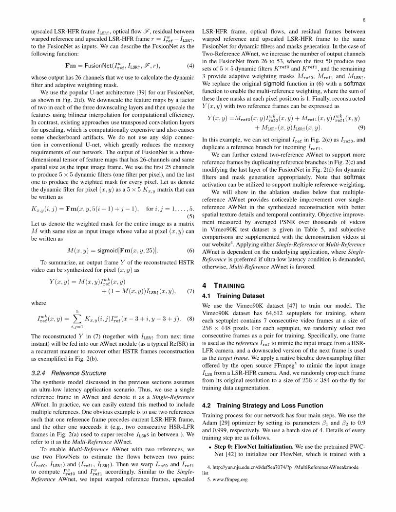
6

upscaled LSR-HFR frame ILSR↑, optical flow F , residual betweenwarped reference and upscaled LSR-HFR frame r = Iwref−ILSR↑,to the FusionNet as inputs. We can describe the FusionNet as thefollowing function:

Fm = FusionNet(Iwref, ILSR↑,F , r), (4)

whose output has 26 channels that we use to calculate the dynamicfilter and adaptive weighting mask.

We use the popular U-net architecture [39] for our FusionNet,as shown in Fig. 2(d). We downscale the feature maps by a factorof two in each of the three downscaling layers and then upscale thefeatures using bilinear interpolation for computational efficiency.In contrast, existing approaches use transposed convolution layersfor upscaling, which is computationally expensive and also causessome checkerboard artifacts. We do not use any skip connec-tion in conventional U-net, which greatly reduces the memoryrequirements of our network. The output of FusionNet is a three-dimensional tensor of feature maps that has 26-channels and samespatial size as the input image frame. We use the first 25 channelsto produce 5× 5 dynamic filters (one filter per pixel), and the lastone to produce the weighted mask for every pixel. Let us denotethe dynamic filter for pixel (x, y) as a 5× 5 Kx,y matrix that canbe written as

Kx,y(i, j) = Fm(x, y, 5(i− 1) + j − 1), for i, j = 1, . . . , 5.(5)

Let us denote the weighted mask for the entire image as a matrixM with same size as input image whose value at pixel (x, y) canbe written as

M(x, y) = sigmoid[Fm(x, y, 25)]. (6)

To summarize, an output frame Y of the reconstructed HSTRvideo can be synthesized for pixel (x, y) as

Y (x, y) = M(x, y)Iwkref(x, y)

+ (1−M(x, y))ILSR↑(x, y), (7)

where

Iwkref(x, y) =

5∑i,j=1

Kx,y(i, j)Iwref(x− 3 + i, y − 3 + j). (8)

The reconstructed Y in (7) (together with ILSR↑ from next timeinstant) will be fed into our AWnet module (as a typical RefSR) ina recurrent manner to recover other HSTR frames reconstructionas exemplified in Fig. 2(b).

3.2.4 Reference StructureThe synthesis model discussed in the previous sections assumesan ultra-low latency application scenario. Thus, we use a singlereference frame in AWnet and denote it as a Single-ReferenceAWnet. In practice, we can easily extend this method to includemultiple references. One obvious example is to use two referencessuch that one reference frame precedes current LSR-HFR frame,and the other one succeeds it (e.g., two consecutive HSR-LFRframes in Fig. 2(a) used to super-resolve ILSRs in between ). Werefer to it as the Multi-Reference AWnet.

To enable Multi-Reference AWnet with two references, weuse two FlowNets to estimate the flows between two pairs:(Iref0, ILSR↑) and (Iref1, ILSR↑). Then we warp Iref0 and Iref1to compute Iwref0 and Iwref1 accordingly. Similar to the Single-Reference AWnet, we input warped reference frames, upscaled

LSR-HFR frame, optical flows, and residual frames betweenwarped reference and upscaled LSR-HFR frame to the sameFusionNet for dynamic filters and masks generation. In the case ofTwo-Reference AWnet, we increase the number of output channelsin the FusionNet from 26 to 53, where the first 50 produce twosets of 5× 5 dynamic filters Kref0 and Kref1, and the remaining3 provide adaptive weighting masks Mref0, Mref1 and MLSR↑.We replace the original sigmoid function in (6) with a softmaxfunction to enable the multi-reference weighting, where the sum ofthese three masks at each pixel position is 1. Finally, reconstructedY (x, y) with two reference frames can be expressed as

Y (x, y) =Mref0(x, y)Iwkref0(x, y) +Mref1(x, y)Iwk

ref1(x, y)

+MLSR↑(x, y)ILSR↑(x, y). (9)

In this example, we can set original Iref in Fig. 2(c) as Iref0, andduplicate a reference branch for incoming Iref1.

We can further extend two-reference AWnet to support morereference frames by duplicating reference branches in Fig. 2(c) andmodifying the last layer of the FusionNet in Fig. 2(d) for dynamicfilters and mask generation appropriately. Note that softmaxactivation can be utilized to support multiple reference weighting.

We will show in the ablation studies below that multiple-reference AWnet provides noticeable improvement over single-reference AWNet in the synthesized reconstruction with betterspatial texture details and temporal continuity. Objective improve-ment measured by averaged PSNR over thousands of videosin Vimeo90K test dataset is given in Table 5, and subjectivecomparisons are supplemented with the demonstration videos atour website4. Applying either Single-Reference or Multi-ReferenceAWnet is dependent on the underlying application, where Single-Reference is preferred if ultra-low latency condition is demanded,otherwise, Multi-Reference AWnet is favored.

4 TRAINING

4.1 Training Dataset

We use the Vimeo90K dataset [47] to train our model. TheVimeo90K dataset has 64,612 septuplets for training, whereeach septuplet contains 7 consecutive video frames at a size of256 × 448 pixels. For each septuplet, we randomly select twoconsecutive frames as a pair for training. Specifically, one frameis used as the reference Iref to mimic the input image from a HSR-LFR camera, and a downscaled version of the next frame is usedas the target frame. We apply a native bicubic downsampling filteroffered by the open source FFmpeg5 to mimic the input imageILSR from a LSR-HFR camera. And, we randomly crop each framefrom its original resolution to a size of 256 × 384 on-the-fly fortraining data augmentation.

4.2 Training Strategy and Loss Function

Training process for our network has four main steps. We use theAdam [29] optimizer by setting its parameters β1 and β2 to 0.9and 0.999, respectively. We use a batch size of 4. Details of everytraining step are as follows.• Step 0: FlowNet Initialization. We use the pretrained PWC-

Net [42] to initialize our FlowNet, which is trained with a

4. http://yun.nju.edu.cn/d/def5ea7074/?p=/MultiReferenceAWnet&mode=list

5. www.ffmpeg.org

7

TABLE 2Objective Performance Comparison of Super-Resolution Methods on

Vimeo90K Dataset [47].

Methods 4× 8×PSNR SSIM PSNR SSIM

SR EDSR [33] 33.11 0.9413 28.20 0.8702ToFlow-SR [47] 33.08 0.9417 - -

RefSRPM [7] 35.06 0.9670 31.30 0.9380

CrossNet [51] 39.17 0.9852 36.15 0.9766AWnet 39.88 0.9862 36.63 0.9768

TABLE 3Objective Performance Comparison of Frame Interpolation using

Vimeo90K [47] (downscaled 4th frame used as reference in AWnet).

PSNR SSIMToFlow-Intp. [47] 33.46 0.9615

AWnet with 1/64 reference 36.63 0.9768AWnet with 1/16 reference 39.88 0.9862

large set of data with ground truth optical flow. The inputs ofPWC-Net are two consecutive frames at the same resolution.

• Step 1: FlowNet Fine-tuning. The reference frame Iref andlow-resolution target frame ILSR have a large gap in theirsizes. Thus, we implement a fine-tuning step to improve theFlowNet. First, we upscale ILSR to ILSR↑ with the same sizeas Iref. Then we compute optical flow between ILSR↑ andIref using PWC-Net. The computed optical flow F is thenused to warp Iref and produce Iwref. Then we apply an `1norm-based warping loss to fine-tune the FlowNet, which isshown below:

Lwarp = ||Igt − Iwref||1, (10)

where Igt is the high-resolution ground truth of ILSR. A smalllearning rate of 1e− 6 is used to fine-tune the FlowNet with40k iterations. A similar loss function has been used in [23].

• Step 2: FusionNet Pretraining. A pretraining step is alsoused for FusionNet. To train the FusionNet, we fix theFlowNet and let the network select appropriate parametersfor FusionNet during training. We use an `1 loss between theoutput Y and the ground truth Igt, given as

Lrec = ||Igt − Y ||1. (11)

We set the learning rate to 1e − 4 and train the network for100k iterations, according to our extensive simulation studies.

• Step 3: End-to-End Joint Training. Starting with ourpretrained models, we jointly train FlowNet and FusionNetby minimizing the same end-to-end `1 loss in (11). In thisstep, we set learning rate to 10−5 for FusionNet and 3×10−6

for FlowNet over 100k iterations. With such pre- and joint-training, network model can converge faster with more robustand reliable behavior.

All networks are implemented and verified using PyTorch. Insubsequent sections, we describe the experiments we performed toevaluate different aspects of proposed AWnet for our dual camerasystem.

5 EXPERIMENTS

We conduct experiments on two types of videos. One type isthe “simulation data” that has images/videos from the existing

and public accessible datasets (e.g., Vimeo90K, KITTI, Flower,LFVideo and Stanford Light Field datasets); the other type isthe “real data” captured by real cameras (e.g., iPhone 7 andGrasshopper3 cameras) under different settings.

5.1 Performance Comparison using Simulation Data

We first compare our method with the state-of-the-art SISRmethod EDSR [33], task-oriented video super-resolution methodToFlow-SR [47], conventional RefSR patchmatch (PM) [7], andthe state-of-the-art learning-based RefSR CrossNet [51]. To befair, we retrain CrossNet with our dataset following the trainingstrategy suggested in [51].

Super-resolution: We first use the test set with 7,824 septu-plets from Vimeo90K [47] for performance comparison. We selectthe fourth image in each septuplet for evaluation following thesuggestion in [4], [47]. For video super-resolution method, theinput is the downscaled septuplet sequence and the target is thesuper-resolved fourth frame. For a single frame or image RefSR,we downscale the fourth frame and use the fifth frame as thereference frame. The results are presented in Table 2. We usePSNR and Structural Similarity (SSIM) [44] as our performancemetrics for evaluation. Results show that our method has superiorperformance in both PSNR and SSIM for 4× super-resolutionalong both spatial dimensions. For PSNR, it yields ≈ 0.7 dB, 4.8dB, 6.8 dB, and 6.7 dB gains against CrossNet, PM, ToFlow-SR,and EDSR, respectively. Similar gains are produced for 8× super-resolution factor, demonstrating the generalization of our work tovarious application scenarios.

In addition to the experiments using Vimeo90K testing sam-ples, we also tested other datasets such as KITTI, Flower, LFVideoand Stanford Light Field data to evaluate the performance of ourproposed AWnet. We discuss those experiments in Section 6 wherewe analyze the impact of camera parallax.

Frame interpolation: Our AWnet can also be used to inter-polate missing intermediate frames (usually at high spatial reso-lution) with the help from another LSR-HFR input. Such frameinterpolation is also supported by optical flow based methods,such as ToFlow-Intp in [47]. We use the third and the fifthframes from the testing septuplets to interpolate missing fourthframe. But for our method, we downscale fourth frame (e.g., 8×resolution downscaling at both spatial dimension) as another input.The results in Table 3 suggest that even a thumbnail-size imageof its original source (e.g., 1/8 × 1/8 the size of the originalimage), can improve the quality of the interpolated intermediateframe significantly. A remarkable 6.4 dB PSNR gain is recordedcompared to ToFlow-Intp [47] when scaling the fourth image toits 1/4×1/4 size (i.e., 16× fewer pixels) and 3.2 dB PSNR gainsfor the case when scaling fourth image to its 1/8× 1/8 size (i.e.,64× fewer pixels).

Model efficiency: Our AWnet demands less system resourcewith less space and time complexity requirements. For example,AWnet model has 109.5 MB parameters, about 25% reductionwhen compared with the CrossNet model at a size of 140.8 MBparameters. When upscaling a snapshot at a factor of 8× spatiallyto the size of 640×448, AWnet consumes about 0.12 second with1499 MB running memory (e.g., about 60% reduction againstthe running memory consumption of CrossNet), while CrossNetis about 0.18 second with 4511 MB running memory. As ancomparative anchor, traditional PM [7] uses 55.9 seconds due toiterative patch match.

8

(a) (b) (c) (d) (e)

Fig. 3. Dual Camera Alignment. (a) HSR-LFR frame Iref; (b) LSR-HFRframe ILSR; (c) HSR-LFR frame Iref frame warped using optical flowonly; (d) HSR-LFR frame Iref warped using mesh-based homography;(e) HSR-LFR frame warped using both mesh-based homography andoptical flow. (a) and (b) are captured using dual iPhone 7 with differentviews.

(a) (b)

(g) (h)(e) (f)

(c) (d)

Fig. 4. Synthesized Quality and Weighting Map W . (a) to (d) are ex-emplified for Vimeo90K simulation data: (a) is the up-scaled ILSR↑ usingbicubic method from ILSR by 8× for both spatial dimensions; (b) is thewarped reference frame Iwref; (c) is the output synthesized frame Y ; (d)is the adaptive weighting mapW on (b); (e) to (h) are the visualization forcamera captured real data with 3× resolution scaling from ILSR to ILSR↑:(e) is the up-scaled image ILSR↑ from the captured LSR-HFR frame; (f)is the warped reference frame Iwref; (g) is the output synthesized frameY ; (h) is the adaptive weighting map W on (f).

5.2 Performance Studies using Real DataWe perform the real video data capture using dual iPhone 7 andGrasshopper3 cameras. One represents a consumer mobile cameraused massively and the other one a camera commonly used forscientific or industrial imaging applications.

5.2.1 Camera AlignmentDual camera setup requires careful calibration to map their relativecoordinates and poses; especially, if we move the system aroundfor shooting different scenes. As suggested by [34], we choosemesh-based homography for alignment. which greatly improvesthe accuracy of subsequent optical flow derivation as shownin Fig. 3. More specifically, we extract SURF features [6] forboth HSR-LFR and LSR-HFR frames, and then use the matchedfeature points to derive the homography transformation matrixfor alignment. Fig. 3(c) shows that optical flow-based alignment

(a) Y with σ2 = 0 (b) Y with σ2 = 0.001 (c) Y with σ2 = 0.01

(d) W with σ2 = 0 (e) W with σ2 = 0.001 (f) W with σ2 = 0.01

Fig. 5. Noise Regularization. (a)-(c) Reconstructions of synthesizedY with noise level σ2 at 0, 0.001 and 0.01; (d)-(f) Weighting map Wwith noise level σ2 at 0, 0.001 and 0.01. Video frames are capturedusing dual iPhone 7. Noise regularization shifts more weights to Iwref ingeneral to improve the image quality, especially for those backgroundstationary areas. But for those regions with occlusions (edge of theathletes), motion blurs (soccer ball) and warping artifacts (grassland),reconstruction still prefers pixels from ILSR↑ to minimize the training loss.Ghosting artifact appear around the player’s head in (b, c), which occurif the AWnet selects blurry regions from ILSR↑ for the pixels that are notcorrectly aligned in Iwref.

fails to produce a good image. We then show the HSR-LFRframe aligned using the mesh-based homography in Fig. 3(d).Fig. 3(e) reveals that homography-based alignment followed byoptical flow-based refinement greatly improves the image quality.

In temporal dimension, for dual iPhone 7 configuration, we usea millisecond timer to synchronize two cameras. Synchronizationwith industrial cameras is much easier where we can apply thehardware clock timer.

Our dual camera system is connected to a high performancecomputer for both HSR-LFR and LSR-HFR video caching. Thecomputer is using an Intel Xeon E5-2620 running at 2.10 GHzwith a GeForce GTX 1080Ti GPU. Without any platform andalgorithmic optimization, it now takes about 7.4 seconds to syn-thesize a 3840 × 2160 frame from a pair of 1280 × 720 framesat 240FPS and 3840× 2160 at 30FPS videos.

5.2.2 Noise RegularizationWe first directly applied our model on data captured with realcamera, but we found that the quality of synthesized images wasnot as good as we had in the case of simulation data, as shownin Fig. 4 (see (c) versus (g)). We observe that the reconstructionof data captured with iPhone 7 camera is blurry in Fig. 4(g), eventhough the reference image after warping retains sharp details, asshown in Fig. 4(f).

Recall that the synthesized video frame Y in (7) is a weightedcombination of the warped reference Iwref and upscaled LSR-HFRinput ILSR↑. The relative weighting factor describing the weightcontribution from the warped reference for a pixel at (x, y)-thposition can be written as

W (x, y) =

M(x, y)∑5

i,j=1Kx,y(i, j)

(1−M(x, y)) +M(x, y)∑5

i,j=1Kx,y(i, j). (12)

Note that the value of W (x, y) lies within [0, 1]. The largerthe W (x, y) is, the more the Iwref contributes and vice versa. Asrevealed in Fig. 4(e), and Fig. 4(f), our model shifts more weightsto ILSR↑, rather Iwref for captured real image synthesis, resulting inover smoothed reconstruction of Y .

9

We also observe that Iwref in Fig. 4(f) not only preserves thesharp details but also the rich colors compared to Y in Fig. 4(g).One potential cause for this is that the camera parameters adjustautomatically during recording to improve the image quality (e.g.,ISO setting, aperture size, etc.). Therefore, the resulting LSR-HFRvideo has a narrow dynamic range and low SNR, as shown inFig. 4(e) versus Fig. 4(f) from an associated HSR-LFR camera. Inanother words, the overall quality of ILSR (or ILSR↑) is much worsecompared to the corresponding Iref (or Iwref).

In the case of simulation data, we do not face this problembecause both ILSR and Iref are generated from the same groundtruth. Such phenomena are also observed when using other RefSRmethods (e.g., PM, CrossNet) to super-resolve real data. The dif-ferences between the simulated data and the real sensor data affectthe accuracy of optical flow and the performance of FusionNet.The FusionNet relies on the similarity between ILSR↑ and Iwref tocombine them. The higher resolution of real sensor data and thedifference between camera parameters cause errors in optical flowestimation and mislead the FusionNet to pay less attention to Iwrefas shown in Fig. 4(h). Thus, it seems that models trained using“clean” simulation data can not be directly extended to cameracaptured real data.

To apply our model on real data, we formulate a “regular-ization” problem that searches for a better weighting factor Wbetween ILSR↑ and Iwref in (7). We propose to add noise n in ILSR↑for regularization during the training progress. Thus, end-to-endlearning optimization in (11) can be updated using regularizedY and Iwref. The only difference here is that instead of usingnoiseless ILSR↑, we inject noise and use ILSR↑ + n in all thecomputations. With such noise regularization on ILSR↑, networklearns to shift more weights to Iwref to improve the quality ofsynthesized reconstruction. Adding synthetic noise at the time oftraining provides robustness and acts as data augmentation [15],[16], [19], [26], [38], [46], [48], [52].

We train our network with Gaussian noise at different vari-ances σ2s, e.g., 0, 0.001, and 0.01. Snapshots of reconstructed Yand weighting factor W with various σ2s are shown in Fig. 5.More comparisons can be seen in the supplementary material. Wecan see that reconstruction shifts more weights to Iwref (e.g., ele-ments in W gets closer to 1 in Fig. 5(d)–(f) as the noise increases(i.e., σ2 increases), yielding better image quality with higherdynamic range, better color and sharper details (see Fig. 5(a)–(c)).Misalignment due to camera parallax and occlusions can introduceartifacts in the recovered images as can be seen around the player’shead. If we increase σ2 further, the quality of images deteriorates.Therefore, to demonstrate the effect of noise regularization, weapply the noise regularization with σ2 = 0.01 for all evaluationsand comparisons in subsequent sections.

5.2.3 Subjective Evaluation

For data captured with the real cameras, we compare the per-formance of our method with the EDSR [33], PM [7]6, andCrossNet [51].

Super-Resolution. Dual iPhone 7 cameras are used in thisstudy. One camera captures a 4K video at 30FPS as the HSR-LFRinput, and the other synchronized camera records 720p video at240FPS as the LSR-HFR input.

6. Because the size of camera captured video frame is larger than thesimulation content in Vimeo90K, we enlarge the patch size from 8 to 16 andsearch range from 16 to 64 for patch matching.

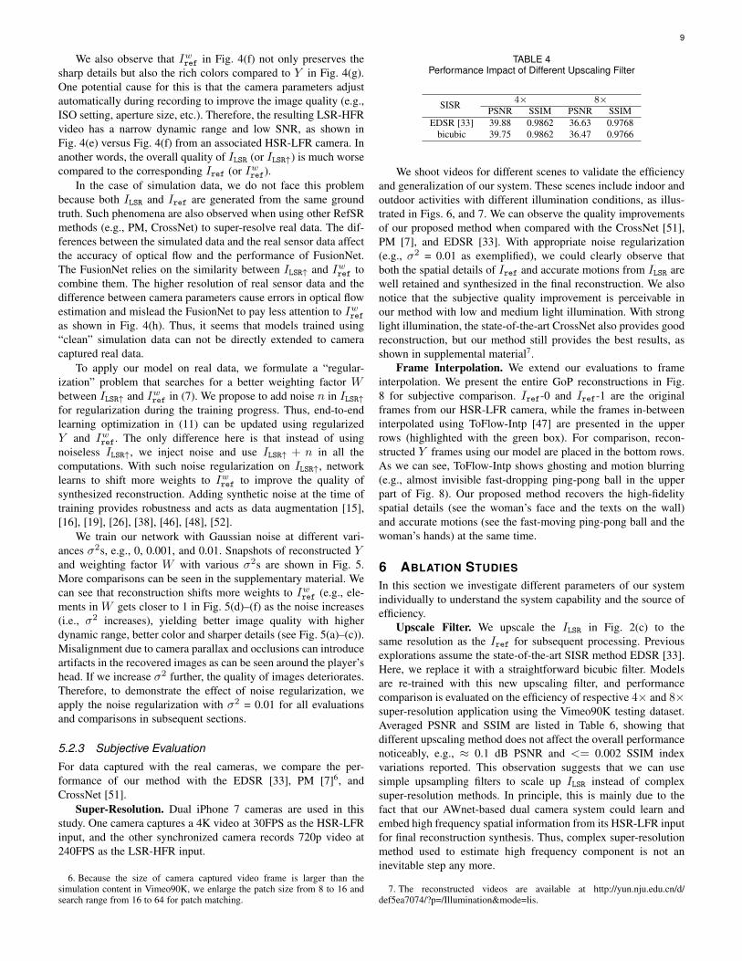
TABLE 4Performance Impact of Different Upscaling Filter

SISR 4× 8×PSNR SSIM PSNR SSIM

EDSR [33] 39.88 0.9862 36.63 0.9768bicubic 39.75 0.9862 36.47 0.9766

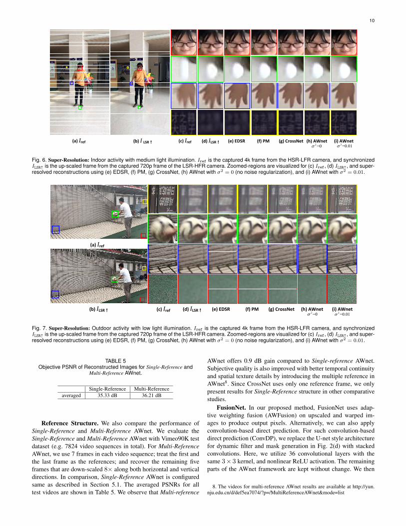
We shoot videos for different scenes to validate the efficiencyand generalization of our system. These scenes include indoor andoutdoor activities with different illumination conditions, as illus-trated in Figs. 6, and 7. We can observe the quality improvementsof our proposed method when compared with the CrossNet [51],PM [7], and EDSR [33]. With appropriate noise regularization(e.g., σ2 = 0.01 as exemplified), we could clearly observe thatboth the spatial details of Iref and accurate motions from ILSR arewell retained and synthesized in the final reconstruction. We alsonotice that the subjective quality improvement is perceivable inour method with low and medium light illumination. With stronglight illumination, the state-of-the-art CrossNet also provides goodreconstruction, but our method still provides the best results, asshown in supplemental material7.

Frame Interpolation. We extend our evaluations to frameinterpolation. We present the entire GoP reconstructions in Fig.8 for subjective comparison. Iref-0 and Iref-1 are the originalframes from our HSR-LFR camera, while the frames in-betweeninterpolated using ToFlow-Intp [47] are presented in the upperrows (highlighted with the green box). For comparison, recon-structed Y frames using our model are placed in the bottom rows.As we can see, ToFlow-Intp shows ghosting and motion blurring(e.g., almost invisible fast-dropping ping-pong ball in the upperpart of Fig. 8). Our proposed method recovers the high-fidelityspatial details (see the woman’s face and the texts on the wall)and accurate motions (see the fast-moving ping-pong ball and thewoman’s hands) at the same time.

6 ABLATION STUDIES

In this section we investigate different parameters of our systemindividually to understand the system capability and the source ofefficiency.

Upscale Filter. We upscale the ILSR in Fig. 2(c) to thesame resolution as the Iref for subsequent processing. Previousexplorations assume the state-of-the-art SISR method EDSR [33].Here, we replace it with a straightforward bicubic filter. Modelsare re-trained with this new upscaling filter, and performancecomparison is evaluated on the efficiency of respective 4× and 8×super-resolution application using the Vimeo90K testing dataset.Averaged PSNR and SSIM are listed in Table 6, showing thatdifferent upscaling method does not affect the overall performancenoticeably, e.g., ≈ 0.1 dB PSNR and <= 0.002 SSIM indexvariations reported. This observation suggests that we can usesimple upsampling filters to scale up ILSR instead of complexsuper-resolution methods. In principle, this is mainly due to thefact that our AWnet-based dual camera system could learn andembed high frequency spatial information from its HSR-LFR inputfor final reconstruction synthesis. Thus, complex super-resolutionmethod used to estimate high frequency component is not aninevitable step any more.

7. The reconstructed videos are available at http://yun.nju.edu.cn/d/def5ea7074/?p=/Illumination&mode=lis.

10

(d) ILSR↑ (e) EDSR (f) PM (g) CrossNet (h) AWnet2=0

(i) AWnet2=0.01

(b) I LSR↑(a) Iref (c) Iref

Fig. 6. Super-Resolution: Indoor activity with medium light illumination. Iref is the captured 4k frame from the HSR-LFR camera, and synchronizedILSR↑ is the up-scaled frame from the captured 720p frame of the LSR-HFR camera. Zoomed-regions are visualized for (c) Iref, (d) ILSR↑, and super-resolved reconstructions using (e) EDSR, (f) PM, (g) CrossNet, (h) AWnet with σ2 = 0 (no noise regularization), and (i) AWnet with σ2 = 0.01.

(e) EDSR (f) PM (g) CrossNet (h) AWnet2 =0

(i) AWnet 2=0.01

(a) Iref

(c) Iref  (d) ILSR↑(b) ILSR↑

Fig. 7. Super-Resolution: Outdoor activity with low light illumination. Iref is the captured 4k frame from the HSR-LFR camera, and synchronizedILSR↑ is the up-scaled frame from the captured 720p frame of the LSR-HFR camera. Zoomed-regions are visualized for (c) Iref, (d) ILSR↑, and super-resolved reconstructions using (e) EDSR, (f) PM, (g) CrossNet, (h) AWnet with σ2 = 0 (no noise regularization), and (i) AWnet with σ2 = 0.01.

TABLE 5Objective PSNR of Reconstructed Images for Single-Reference and

Multi-Reference AWnet.

Single-Reference Multi-Referenceaveraged 35.33 dB 36.21 dB

Reference Structure. We also compare the performance ofSingle-Reference and Multi-Reference AWnet. We evaluate theSingle-Reference and Multi-Reference AWnet with Vimeo90K testdataset (e.g. 7824 video sequences in total). For Multi-ReferenceAWnet, we use 7 frames in each video sequence; treat the first andthe last frame as the references; and recover the remaining fiveframes that are down-scaled 8× along both horizontal and verticaldirections. In comparison, Single-Reference AWnet is configuredsame as described in Section 5.1. The averaged PSNRs for alltest videos are shown in Table 5. We observe that Multi-reference

AWnet offers 0.9 dB gain compared to Single-reference AWnet.Subjective quality is also improved with better temporal continuityand spatial texture details by introducing the multiple reference inAWnet8. Since CrossNet uses only one reference frame, we onlypresent results for Single-Reference structure in other comparativestudies.

FusionNet. In our proposed method, FusionNet uses adap-tive weighting fusion (AWFusion) on upscaled and warped im-ages to produce output pixels. Alternatively, we can also applyconvolution-based direct prediction. For such convolution-baseddirect prediction (ConvDP), we replace the U-net style architecturefor dynamic filter and mask generation in Fig. 2(d) with stackedconvolutions. Here, we utilize 36 convolutional layers with thesame 3× 3 kernel, and nonlinear ReLU activation. The remainingparts of the AWnet framework are kept without change. We then

8. The videos for multi-reference AWnet results are available at http://yun.nju.edu.cn/d/def5ea7074/?p=/MultiReferenceAWnet&mode=list

11

AWnet σ2=0.01

Iref‐0 Iref‐1ToFlow‐Intp

Fig. 8. Frame interpolation. Indoor activity with medium light illumination. The most left and the most right of first rows are the captured HSR-LFR frames. Seven frames in-between are interpolated using ToFlow-Intp [47]; The second rows are the synthesized HSTR frames using ourAWnet, which is trained with noise regularization with the variance of 0.01. Zoom in the pictures, and you will see more image details. (More insupplemental material.)

TABLE 6Objective Comparison between Adaptive Weighting Fusion and

Convolution-based Direct Prediction for Output Pixel Reconstruction.

4× 8×PSNR SSIM PSNR SSIM

AWFusion 39.88 0.9862 36.63 0.9768ConvDP 39.67 0.9856 36.45 0.9756

evaluate the default AWFusion and ConvDP using the Vimeo90Ktest dataset (e.g., 7824 video sequences in total). Table 6 providesthe averaged PSNR and SSIM results of the reconstructions usingrespective methods. Although the quantitative gains in terms ofPSNR and SSIM are not very large, Fig. 9 shows noticeablequality improvement of synthesized frame with less noise andsharp/clear reconstruction for the AWFusion compared to ConvDP(e.g., Fig. 9(c) vs (d)).

Camera Parallax. Dual camera setup is used in our system.Thus camera parallax could be an issue that affects the systemperformance. We show in our studies below by using simulationdata from available KITTI [36], Flower [41], LFVideo [43],Stanford light field [1] datasets, and real data captured by ourdual camera system with various parallax settings to demonstratethe robustness of our method.

Comparison Using Simulation Data: We test our AWneton Flower [41], LFVideo [43] and Stanford light field (LegoGantry) [1] datasets following the same configuration in [51].The Flower and LFVideo datasets are light field images cap-

tured using Lytro ILLUM camera. Each light field image has376×541 spatial samples and 14×14 angular samples (grid).The same as the methods applied in [41], [51], we extract thecentral 8×8 grid of angular samples to avoid invalid images.Parallax is offered by setting the reference image Iref at (0,0), and associated low-resolution correspondence at (i, i), with0 < i ≤ 7 by shifting position to another different angularsample. For example, Flower(1,1) and LFVideo(7,7) in Table 7,represent low-resolutions at (1,1) and (7,7) with respect to therespective references at (0,0). Images in both Flower and LFVideodatasets exhibit small parallax settings [41], [51]. On the otherhand, Stanford light field dataset contains the light field imagesshot using a Canon Digital Rebel XTi with a canon 10-22 mmlens. It is placed using a movable Mindstorms motor on theLego gantry, where the parallax is introduced by the baselinedistances along with the camera movement. Under such equipmentsettings, the captured light-field images have much larger parallaxthan those captured by Lytro ILLUM camera. Both Table 7 andTable 8 also shows the leading performance of our proposedAWnet at a variety of parallax between testing and referenceimages, further demonstrating the generalization of our networkin different application scenarios. Especially, on average, up to1.3 dB PSNR improvement is obtained of our AWnet against theCrossNet in Table 8 for large parallax setting. This is mainly due tothe reason that CrossNet was not initially designed for RefSR withlarger parallax. Thus, additional parallax augmentation procedurewas suggested in [51] for re-training.

12

(a) (b) (c) (d) (e)

Fig. 9. Subjective Evaluation of Adaptive Weighting Fusion and Convolution-based Direction Prediction Using Synthetic Vimeo90K Test Dataset.(a) Iref; (b) ILSR; (c) Convolution-based Direct Prediction; (d) Adaptive Weighting Fusion; (e) Ground truth. The upper part is a raining scene withzoomed rain drop and label. The bottom part is a gym scene with zoomed face of a trainee.

TABLE 7Objective Performance Comparison of 4× and 8× Super-Resolution Methods on Flower and LFVideo Datasets

Methods Scale Flower(1,1) Flower(7,7) LFVideo(1,1) LFVideo(7,7)PSNR SSIM PSNR SSIM PSNR SSIM PSNR SSIM

SRCNN [14] 4× 32.76 0.89 32.96 0.90 32.98 0.86 33.27 0.86VDSR [28] 4× 33.34 0.90 33.58 0.91 33.58 0.87 33.87 0.88MDSR [33] 4× 34.40 0.92 34.65 0.92 34.62 0.89 34.91 0.90

PM [7] 4× 38.03 0.97 35.23 0.94 38.22 0.95 37.08 0.94CrossNet [51] 4× 41.23 0.9625 38.09 0.9475 41.57 0.9758 39.17 0.9627

AWnet 4× 41.33 0.9631 38.31 0.9492 41.63 0.9757 39.36 0.9635SRCNN [14] 8× 28.17 0.77 28.25 0.77 29.43 0.75 29.63 0.76VDSR [28] 8× 28.58 0.78 28.68 0.78 29.83 0.77 30.04 0.77MDSR [33] 8× 29.15 0.79 29.26 0.80 30.43 0.78 30.65 0.79

PM [7] 8× 35.26 0.95 30.41 0.85 36.72 0.94 34.48 0.91CrossNet [51] 8× 39.35 0.9571 34.11 0.9149 40.63 0.9727 36.97 0.9465

AWnet 8× 39.29 0.9571 34.53 0.9199 40.48 0.9725 37.25 0.9487

TABLE 8Objective Performance (PSNR) Comparison of 8× Super-Resolution

Methods on Stanford Light Field Dataset

Methods parallax = (1,0) (3,0) (5,0)MDSR [33] 29.66 29.66 29.67

PM [7] 34.61 32.55 30.42CrossNet [51] 39.33 36.77 35.15

AWnet 39.53 37.65 36.47

TABLE 9Performance Evaluation Using KITTI dataset for Super-Resolution

4× 8×PSNR SSIM PSNR SSIM

EDSR [33] 27.03 0.8519 23.47 0.7377CrossNet [51] 27.43 0.8631 24.92 0.7981

AWnet 28.19 0.8882 26.01 0.8356

KITTI dataset has 54cm baseline distance for two cameras.We apply our method and CrossNet with pretrained modelsusing Vimeo90K dataset directly to KITTI test data with 400stereo image pairs. We use the high-resolution left-view imagesas the reference for the low-resolution right-view images. Sinceboth CrossNet and our method expect the image resolution tobe divisible by 64, thus, we crop images to 1216 × 320 fortesting. Table 9 gives the PSNR and SSIM for super-resolutionevaluation. Our method still offers better PSNR (e.g., > 1 dBgain for 8× resolution scaling factor) and SSIM compared to theCrossNet. EDSR results are offered as a reference point, revealingthat RefSR still exhibits superior performance, even with a largecamera parallax (i.e., 54cm baseline in KITTI data). Results inTable 9 and Table 2 suggest that both PSNR and SSIM are droppedsignificantly when evaluating models on KITTI compared to theVimeo90K test data. This is because the introduction of the (large)camera parallax leads to the inaccurate flow estimation for laterprocessing. Similar observations are reported in CrossNet [51]

13

where PSNR and SSIM drop as the camera parallax increases.Comparison Using Real Data: We choose a pair of Grasshop-

per3 cameras to perform more parallax studies due to its easysetup using industrial cameras. We use two Grasshopper3 GS3-U3-51S5C cameras with respective 20mm and 6mm lens installed.There is nearly 4× resolution gap between these two cameras, e.g.,one is at 2304×2048, and the other one is at 576×512. We fix theframe rate of the HSR-LFR camera at 240FPS and the frame rateof the LSR-HFR camera at 30FPS. Viewing distance from thecameras to the scene is about 2 meters, and the baseline distancebetween these two cameras are adjusted at 5cm, 10cm, 15cm,20cm and 25cm for a variety of parallax configurations. Figure 10plots the reconstructed images at different baseline distances. Aswe can see, our system has reliable performance at a variety ofparallax settings. Image quality can be enhanced noticeably withnoise regularization, as shown in enlarged thumbnails in Figure 10.And in the region with repeated patterns, the checkerboard, thereare some ghosts on the results of CrossNet, but our networkdoes not have this problem. Timer digits are over-smoothed byCrossNet, especially for the scenarios with larger baseline distance(e.g., 25cm), but ours still retain the sharp presentation.

Exposure time. The exposure time affects the number ofarrival photons, thus having impacts on the image quality for eachsnapshot and subsequent synthesis performance. Identical dualcamera setup is used as in parallax study, but with the baselinedistance fixed at 4.4cm. We fix the aperture sizes of the twocameras and set the ISO gain to automatic mode.

The exposure time of the HSR-LFR camera is fixed as defaultto record 30FPS reference video with 2304×1920 resolution at30FPS. For comparative studies, We set the exposure time of theLSR-HFR camera to 10ms, 5ms, 2.5ms , 1ms and 0.5ms respec-tively, to record video with 576×480 resolution with 100FPS.Both captured and reconstructed images are shown in Fig. 11.From the captured LSR-HFR frames, we can see that the signal-to-noise ratio (SNR) of the images decrease greatly (Fig. 11(d)) asthe decrease of the exposure time.

Experiments reveal that CrossNet can remove some noise butthe capacity is limited. This may be due to the smoothing effectof global convolutions applied, leading to blurred timing digitsand jewelry contour (see Fig. 11(e)). Our AWnet can effectivelyalleviate the noise (even with strong level) and maintain thesharpness, yielding much high-quality HSTR frames. The noiseinduced by the lower SNR (with shorter exposure time), is greatlyremoved by our method (as illustrated in Fig. 11(d)-(e)), providingvisually pleasant reconstruction with appealing spatial and tempo-ral details. From these snapshots (and zoomed thumbnails), wecan see that our system is robust and reliable to various exposuresettings as well.

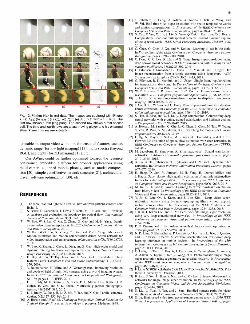
Motion blur. Camera acquisition with insufficient temporalresolution would introduce the motion blur as the zoomed regionsof HSR-LFR frames in Fig. 12(a). Our work is trying to leveragethe LSR-HFR video with accurate motion details to resolve it.Towards this goal, dedicated FlowNet and FusionNet are devisedto extract and aggregate information (see Fig. 2(c)) for adaptiveweighted synthesis. Optical flow extracted by the FlowNet is usedto warp the Iref followed by the dynamic filter and mask generatedby the FusionNet to weigh the respective information from Irefand ILSR appropriately.

As shown in Fig. 12, motion blurs are clearly observed inFig. 12(a) around fast moving objects. Such effect is slightlyreduced in Fig. 12(c) when flow information from LSR-HFR is

utilized to warp the Iref. Further improvement is achieved inFig. 12(d) by utilizing the dynamic filter to restore the textures onblurred objects using information from the LSR-HFR input (seeFig. 12(b)(c)(d)). Sometimes, artifacts are induced due to overfiltering, but subsequent adaptive mask in Fig. 12(e) will thenintelligently combine pixels from ILSR↑ and Iwk

ref for even betterreconstruction shown in Fig. 12(f).

Resolution Gap. An interesting observation is that our modeltrained with image pairs (see Section 4) having 8× resolutiongap (noted as 8×-Model) provides much better reconstructionquality subjectively (Fig. 13(f)) compared to the model trainedusing image pairs with 4× resolution gap (noted as 4×-Model)(Fig. 13(e)). For both models, noise level is set with σ2 = 0.01for regularization. For illustrative comparison, we downscale theIref to its 1

16 th (e.g., 4× downscaling at each spatial dimension)and 1

64 th (e.g., 8× downscaling at each spatial dimension) sizes.Perceptually, a snapshot from the LSR-HFR camera in Fig. 13(d)is close to 8× downscaled Iref in Fig. 13(c), but worse than4× downscaled Iref in Fig. 13(b). Thus, when we use 4×-Model, our network will evenly weigh information from Iref andILSR yielding a smooth reconstruction with moderate quality inFig. 13(e); but for 8×-Model, since the 8× downscaled version intraining is with pretty bad quality, more weights will be given toIref in stationary areas and to ILSR in motion areas for adaptivefusion synthesis, leading to much sharp details in reconstructionas shown in Fig. 13(f). In other words, this is another example ofadaptive weighting between the HSR-LFR and LSR-HFR camerainputs for final reconstruction quality improvement, where thoseweights can be regularized during training using sample pairs withdifferent resolution gaps.

7 CONCLUSION

A dual camera system is developed in this work for high spa-tiotemporal resolution video acquisition where one camera cap-tures the HSR-LFR video, and the other one records the LSR-HFR video. An end-to-end learning framework, AWnet, is thenproposed to learn the spatial and temporal information fromboth camera inputs, and drive the final appealing reconstructionby intelligently synthesizing the content from either HSR-LFRor LSR-HFR frame. Towards this goal, separable FlowNet andFusionNet are devised in our framework, to explicitly exploitthe information from two cameras so as to derive the adaptiveweighting functions for reconstruction synthesis.

Our system demonstrates the superior performance, in compar-ison to the existing works, such as the state-of-the-art CrossNet,PM, EDSR, and ToFlow-SR for super-resolution, and ToFlow-Intpfor frame interpolation, showing noticeable gains both subjectivelyand objectively, using simulation data and camera captured realdata. ew We also analyze various aspects of our system bybreaking down its modular components, such as upscaling filter,reference structure, camera parallax, exposure time, etc. Thesestudies pave the way for the application of our model to differentscenarios.

In general, our system belongs to a hybrid camera or multi-camera category, even though our current emphasis is the pro-duction of video at both high spatial resolution and high framerate. But this approach can be easily extended to view synthesissince the different viewpoints can be also generalized using flowrepresentation. Another interesting avenue is to extend currentRefSR mechanism in AWnet to include more cameras (e.g., > 2)

14

(a) Iref (b) ILSR↑ (d) AWnet σ2=0 (e) AWnet σ2=0.01(c) CrossNet

5cm

25cm

Fig. 10. Camera Parallax. Image reconstruction for our dual camera system when placing cameras with baseline distance at 5cm and 25cm. OurLSR-HFR camera operates at 240FPS. These images are captured using dual Grasshopper3 GS3-U3-51S5C cameras. The frames in the firstcolumn are the captured HSR-LFR frames. The frames in the second column are the captured LSR-HFR frames. Look at the repeated patterns onthe checkerboard snapshots, there are some ghosts on the results of CrossNet because its multi-scale warping in feature domain, but our methoddoes not have this problem. And our method has strong robustness when parallax is large. Zoom in the pictures, you will see more details inthe larger images. More parallax settings in supplemental material.

(c) Iref (d) ILSR↑ (f) AWnet σ2=0.01(e) CrossNet(a) Iref (b) ILSR↑

10ms

0.5ms

Fig. 11. Exposure Time. Various exposure time exemplified using our dual camera system. These images are captured using dual Grasshopper3GS3-U3-51S5C cameras. The frames in the first column are the captured HSR-LFR frames using default exposure, the frames in the second columnare the captured LSR-HFR frames with various exposure adjustments. Noise increases as exposure time decreases. CrossNet could remove somenoise but generally lead to blurred artifacts induced by the global convolutions. Our AWnet can effective remove noise and improve the picturequality greatly. More exposure time settings in supplemental material.

15

(a) (b) (c) (d) (e) (f)

Fig. 12. Motion blur in real data. The images are captured with iPhone7. (a) IHSR; (b) ILSR↑; (c) Iwref; (d) Iwk

ref ; (e) M ; (f) Y with σ2 = 0.01. Thefirst row shows a fast ping-pong. The second row shows a fast soccerball. The third and fourth rows are a fast-moving player and his enlargedshoe. Zoom in to see more details.

to enable the output video with more dimensional features, such asdynamic range (for low light imaging) [13], multi-spectra (beyondRGB), and depth (for 3D imaging) [18], etc.

Our AWnet could be further optimized towards the resourceconstrained embedded platform for broader applications usingmulti-camera equipped mobile phones, such as model compres-sion [20], simple yet effective network structure [21], architecture-driven software optimization [30], etc.

REFERENCES

[1] The (new) stanford light field archive. http://http://lightfield.stanford.edu/lfs.html.

[2] S. Baker, D. Scharstein, J. Lewis, S. Roth, M. J. Black, and R. Szeliski.A database and evaluation methodology for optical flow. InternationalJournal of Computer Vision, 92(1):1–31, 2011.

[3] W. Bao, W.-S. Lai, C. Ma, X. Zhang, Z. Gao, and M.-H. Yang. Depth-aware video frame interpolation. In IEEE Conferene on Computer Visionand Pattern Recognition, 2019.

[4] W. Bao, W.-S. Lai, X. Zhang, Z. Gao, and M.-H. Yang. Memc-net:Motion estimation and motion compensation driven neural network forvideo interpolation and enhancement. arXiv preprint arXiv:1810.08768,2018.

[5] W. Bao, X. Zhang, L. Chen, L. Ding, and Z. Gao. High-order model anddynamic filtering for frame rate up-conversion. IEEE Transactions onImage Processing, 27(8):3813–3826, 2018.

[6] H. Bay, A. Ess, T. Tuytelaars, and L. Van Gool. Speeded-up robustfeatures (surf). Computer vision and image understanding, 110(3):346–359, 2008.

[7] V. Boominathan, K. Mitra, and A. Veeraraghavan. Improving resolutionand depth-of-field of light field cameras using a hybrid imaging system.In 2014 IEEE International Conference on Computational Photography(ICCP), pages 1–10. IEEE, 2014.

[8] D. J. Brady, M. E. Gehm, R. A. Stack, D. L. Marks, D. S. Kittle, D. R.Golish, E. Vera, and S. D. Feller. Multiscale gigapixel photography.Nature, 486(7403):386, 2012.

[9] D. J. Brady, W. Pang, H. Li, Z. Ma, Y. Tao, and X. Cao. Parallel cameras.Optica, 5(2):127–137, Feb 2018.

[10] A. Burton and J. Radford. Thinking in Perspective: Critical Essays in theStudy of Thought Processes. Psychology in progress. Methuen, 1978.

[11] J. Caballero, C. Ledig, A. Aitken, A. Acosta, J. Totz, Z. Wang, andW. Shi. Real-time video super-resolution with spatio-temporal networksand motion compensation. In Proceedings of the IEEE Conference onComputer Vision and Pattern Recognition, pages 4778–4787, 2017.

[12] X. Cao, T. Yue, X. Lin, S. Lin, X. Yuan, Q. Dai, L. Carin, and D. J. Brady.Computational snapshot multispectral cameras: Toward dynamic captureof the spectral world. IEEE Signal Processing Magazine, 33(5):95–108,2016.

[13] C. Chen, Q. Chen, J. Xu, and V. Koltun. Learning to see in the dark.In Proceedings of the IEEE Conference on Computer Vision and PatternRecognition, pages 3291–3300, 2018.

[14] C. Dong, C. C. Loy, K. He, and X. Tang. Image super-resolution usingdeep convolutional networks. IEEE transactions on pattern analysis andmachine intelligence, 38(2):295–307, 2015.

[15] G. Eilertsen, J. Kronander, G. Denes, R. K. Mantiuk, and J. Unger. Hdrimage reconstruction from a single exposure using deep cnns. ACMTransactions on Graphics (TOG), 36(6):1–15, 2017.

[16] G. Eilertsen, R. K. Mantiuk, and J. Unger. Single-frame regularizationfor temporally stable cnns. In Proceedings of the IEEE Conference onComputer Vision and Pattern Recognition, pages 11176–11185, 2019.

[17] W. T. Freeman, T. R. Jones, and E. C. Pasztor. Example-based super-resolution. IEEE Computer graphics and Applications, (2):56–65, 2002.

[18] T. Fujii. 3d image processing–from capture to display–. ElectronicImaging, 2019(3):625–1, 2019.

[19] J. Gu, H. Lu, W. Zuo, and C. Dong. Blind super-resolution with iterativekernel correction. In Proceedings of the IEEE conference on computervision and pattern recognition, pages 1604–1613, 2019.

[20] S. Han, H. Mao, and W. J. Dally. Deep compression: Compressing deepneural networks with pruning, trained quantization and huffman coding.arXiv preprint arXiv:1510.00149, 2015.

[21] A. Howard, M. Sandler, G. Chu, L.-C. Chen, B. Chen, M. Tan, W. Wang,Y. Zhu, R. Pang, V. Vasudevan, et al. Searching for mobilenetv3. arXivpreprint arXiv:1905.02244, 2019.

[22] E. Ilg, N. Mayer, T. Saikia, M. Keuper, A. Dosovitskiy, and T. Brox.Flownet 2.0: Evolution of optical flow estimation with deep networks. InIEEE Conference on Computer Vision and Pattern Recognition (CVPR),Jul 2017.

[23] M. Jaderberg, K. Simonyan, A. Zisserman, et al. Spatial transformernetworks. In Advances in neural information processing systems, pages2017–2025, 2015.

[24] X. Jia, B. De Brabandere, T. Tuytelaars, and L. V. Gool. Dynamic filternetworks. In Advances in Neural Information Processing Systems, pages667–675, 2016.

[25] H. Jiang, D. Sun, V. Jampani, M.-H. Yang, E. Learned-Miller, andJ. Kautz. Super slomo: High quality estimation of multiple intermediateframes for video interpolation. In Proceedings of the IEEE Conferenceon Computer Vision and Pattern Recognition, pages 9000–9008, 2018.

[26] M. Jin, Z. Hu, and P. Favaro. Learning to extract flawless slow motionfrom blurry videos. In Proceedings of the IEEE Conference on ComputerVision and Pattern Recognition, pages 8112–8121, 2019.

[27] Y. Jo, S. Wug Oh, J. Kang, and S. Joo Kim. Deep video super-resolution network using dynamic upsampling filters without explicitmotion compensation. In Proceedings of the IEEE Conference onComputer Vision and Pattern Recognition, pages 3224–3232, 2018.

[28] J. Kim, J. Kwon Lee, and K. Mu Lee. Accurate image super-resolutionusing very deep convolutional networks. In Proceedings of the IEEEconference on computer vision and pattern recognition, pages 1646–1654, 2016.

[29] D. P. Kingma and J. Ba. Adam: A method for stochastic optimization.arXiv preprint arXiv:1412.6980, 2014.

[30] N. D. Lane, S. Bhattacharya, P. Georgiev, C. Forlivesi, L. Jiao, L. Qendro,and F. Kawsar. Deepx: A software accelerator for low-power deeplearning inference on mobile devices. In Proceedings of the 15thInternational Conference on Information Processing in Sensor Networks,page 23. IEEE Press, 2016.

[31] C. Ledig, L. Theis, F. Huszar, J. Caballero, A. Cunningham, A. Acosta,A. Aitken, A. Tejani, J. Totz, Z. Wang, et al. Photo-realistic single imagesuper-resolution using a generative adversarial network. In Proceedingsof the IEEE conference on computer vision and pattern recognition,pages 4681–4690, 2017.

[32] F. Li. A HYBRID CAMERA SYSTEM FOR LOW-LIGHT IMAGING. PhDthesis, University of Delaware, 2011.

[33] B. Lim, S. Son, H. Kim, S. Nah, and K. Mu Lee. Enhanced deep residualnetworks for single image super-resolution. In Proceedings of the IEEEConference on Computer Vision and Pattern Recognition Workshops,pages 136–144, 2017.

[34] S. Liu, L. Yuan, P. Tan, and J. Sun. Bundled camera paths for videostabilization. ACM Transactions on Graphics (TOG), 32(4):78, 2013.

[35] S. Lu. High-speed video from asynchronous camera array. In 2019 IEEEWinter Conference on Applications of Computer Vision (WACV), pages

16

(a) (b) (c) (d) (e) (f)

Fig. 13. Resolution Gap Impact. (a) Iref, (b) Iref with 4× resolution downscaling and upscaling to original size by EDSR, (c) Iref with 8× resolutiondownscaling and upscaling to original size by EDSR, (d) ILSR, (e) Y with 4×-Model, (f) Y with 8×-Model.

2196–2205. IEEE, 2019.[36] M. Menze and A. Geiger. Object scene flow for autonomous vehicles.

In Proceedings of the IEEE Conference on Computer Vision and PatternRecognition, pages 3061–3070, 2015.

[37] S. Niklaus and F. Liu. Context-aware synthesis for video frame interpo-lation. In Proceedings of the IEEE Conference on Computer Vision andPattern Recognition, pages 1701–1710, 2018.

[38] H. Noh, T. You, J. Mun, and B. Han. Regularizing deep neural networksby noise: Its interpretation and optimization. In Advances in NeuralInformation Processing Systems, pages 5109–5118, 2017.

[39] O. Ronneberger, P. Fischer, and T. Brox. U-net: Convolutional networksfor biomedical image segmentation. In International Conference onMedical image computing and computer-assisted intervention, pages234–241. Springer, 2015.

[40] M. S. Sajjadi, R. Vemulapalli, and M. Brown. Frame-recurrent videosuper-resolution. In Proceedings of the IEEE Conference on ComputerVision and Pattern Recognition, pages 6626–6634, 2018.

[41] P. P. Srinivasan, T. Wang, A. Sreelal, R. Ramamoorthi, and R. Ng.Learning to synthesize a 4d rgbd light field from a single image. InProceedings of the IEEE International Conference on Computer Vision,pages 2243–2251, 2017.

[42] D. Sun, X. Yang, M.-Y. Liu, and J. Kautz. Pwc-net: Cnns for opticalflow using pyramid, warping, and cost volume. In Proceedings of theIEEE Conference on Computer Vision and Pattern Recognition, pages8934–8943, 2018.

[43] T.-C. Wang, J.-Y. Zhu, N. K. Kalantari, A. A. Efros, and R. Ramamoorthi.Light field video capture using a learning-based hybrid imaging system.ACM Transactions on Graphics (TOG), 36(4):133, 2017.

[44] Z. Wang, A. C. Bovik, H. R. Sheikh, E. P. Simoncelli, et al. Imagequality assessment: from error visibility to structural similarity. IEEEtransactions on image processing, 13(4):600–612, 2004.

[45] G. Wu, B. Masia, A. Jarabo, Y. Zhang, L. Wang, Q. Dai, T. Chai, andY. Liu. Light field image processing: An overview. IEEE Journal ofSelected Topics in Signal Processing, 11(7):926–954, 2017.

[46] Q. Xie, E. Hovy, M.-T. Luong, and Q. V. Le. Self-training with noisy stu-dent improves imagenet classification. arXiv preprint arXiv:1911.04252,2019.

[47] T. Xue, B. Chen, J. Wu, D. Wei, and W. T. Freeman. Video enhancementwith task-oriented flow. International Journal of Computer Vision(IJCV), 127(8):1106–1125, 2019.

[48] K. Zhang, W. Zuo, and L. Zhang. Deep plug-and-play super-resolutionfor arbitrary blur kernels. In Proceedings of the IEEE Conference onComputer Vision and Pattern Recognition, pages 1671–1681, 2019.

[49] H. Zheng, M. Guo, H. Wang, Y. Liu, and L. Fang. Combiningexemplar-based approach and learning-based approach for light fieldsuper-resolution using a hybrid imaging system. In Proceedings of theIEEE International Conference on Computer Vision, pages 2481–2486,2017.

[50] H. Zheng, M. Ji, H. Wang, Y. Liu, and L. Fang. Learning cross-scalecorrespondence and patch-based synthesis for reference-based super-resolution. In BMVC, 2017.

[51] H. Zheng, M. Ji, H. Wang, Y. Liu, and L. Fang. Crossnet: An end-to-endreference-based super resolution network using cross-scale warping. InProceedings of the European Conference on Computer Vision (ECCV),pages 88–104, 2018.

[52] S. Zheng, Y. Song, T. Leung, and I. Goodfellow. Improving therobustness of deep neural networks via stability training. In Proceedingsof the ieee conference on computer vision and pattern recognition, pages4480–4488, 2016.

17

Ming Cheng is a Ph.D. candidate of ElectricalEngineering with the Institute of Image Com-munication and Network Engineering, ShanghaiJiao Tong University, Shanghai, China. She re-ceived the B.S. degree in the University of Elec-tronic Science and Technology of China, China,in 2016. Her research interests include computervision, video processing and multi-cameras.

Zhan Ma (SM’19) is now on the faculty of Elec-tronic Science and Engineering School, NanjingUniversity, Jiangsu, 210093, China. He receivedthe B.S. and M.S. from Huazhong Universityof Science and Technology (HUST), Wuhan,China, in 2004 and 2006 respectively, and thePh.D. degree from the New York University, NewYork, in 2011. From 2011 to 2014, he has beenwith Samsung Research America, Dallas TX,and Futurewei Technologies, Inc., Santa Clara,CA, respectively. His current research focuses

on the next-generation video coding, energy-efficient communication,gigapixel streaming and deep learning. He is a co-recipient of 2018ACM SIGCOMM Student Research Competition Finalist, 2018 PCMBest Paper Finalist, and 2019 IEEE Broadcast Technology Society BestPaper Award.

M. Salman Asif is currently an Assistant Pro-fessor in the Department of Electrical and Com-puter Engineering at the University of Califor-nia, Riverside. Prior to joining UC Riverside, hewas a postdoctoral research associate in theDSP group at Rice University. Before that hebriefly worked as a Research Engineer at Sam-sung Research America, Dallas. He receivedthe Ph.D. at the Georgia Institute of Technologyunder the supervision of Justin Romberg. Hisresearch interests broadly lie in the areas of

information processing and computational sensing with applications insignal processing, machine learning, and computational imaging.

Yiling Xu is a full researcher of School ofElectronic Information and Electronic Engineer-ing, Shanghai Jiao Tong University, Shanghai,200145, China. She received the B.S., M.S. andPh.D. from the University of Electronic Scienceand Technology of China, China, in 1999, 2001and 2004 respectively. From 2004 to 2013, shewas with Multimedia Communication ResearchInstitute of Samsung Electronics Inc, Korea. Hermain research interests include architecture de-sign for next generation multimedia systems, dy-

namic data encapsulation, adaptive cross layer design, dynamic adap-tion for heterogenous networks and N-screen content presentation.

Haojie Liu is a Ph.D candidate in School of Elec-tronic Science and Engineering, Nanjing Univer-sity, Nanjing, China. He received the B.S degreein Nanjing University in 2016. His research inter-ests includes video communication and process-ing, machine learning and computer vision.

Wenbo Bao is a Ph.D. candidate of ElectricalEngineering with the Institute of Image Com-munication and Network Engineering, ShanghaiJiao Tong University, Shanghai, China. He re-ceived the B.S. degree in Electronic InformationEngineering from Huazhong University of Sci-ence and Technology, Hubei, China, in 2014.His research interests include computer vision,machine learning, and video processing.

Jun Sun is currently a professor and Ph.D.advisor of Shanghai Jiao Tong University. Hereceived his B.S. in 1989 from University ofElectronic Sciences and technology of China,Chengdu, China, and a Ph.D. degree in 1995from Shanghai Jiao Tong University, all in electri-cal engineering. In 1996, he was elected as themember of HDTV Technical Executive ExpertsGroup (TEEG) of China. Since then, he hasbeen acting as one of the main technical expertsfor the Chinese government in the field of digital

television and multimedia communications. In the past five years, he hasbeen responsible for several national projects in DTV and IPTV fields. Hehas published over 50 technical papers in the area of digital televisionand multimedia communications and received 2nd Prize of NationalSci. & Tech. Development Award in 2003, 2008. His research interestsinclude digital television, image communication, and video encoding.