1

A Guided Tour of Several New and Interesting Routing Problems

by

Bruce Golden, University of Maryland

Edward Wasil, American University

Presented at NOW 2006Saint-Rémy de Provence, August 2006

2

Outline of Lecture

The close enough traveling salesman problem (CETSP)

The CETSP over a street network

The colorful traveling salesman problem (CTSP)

The consistent vehicle routing problem (CVRP)

Conclusions

3

My Student Collaborators

Chris GroerDamon Gulczynski Jeff HeathCarter PriceRobert ShuttleworthYupei Xiong

4

Until recently, utility meter readers had to visit each customer location and read the meter at that site

Now, radio frequency identification (RFID) technology allows the meter reader to get close to each customer and remotely read the meter

A simple model

Customers are points in Euclidean space

There is a central depot

There is a fixed radius r which defines “close enough”

The goal is to minimize distance traveled

The Close Enough Traveling Salesman Problem

5

Create a set S of “supernodes” such that each customer is within r units of at least one supernode

This set should be as small in cardinality as possible

Solve the TSP over S and the central depot

Use post-processing to reposition the supernodes in order to reduce total distance

An illustration follows

CETSP Heuristic

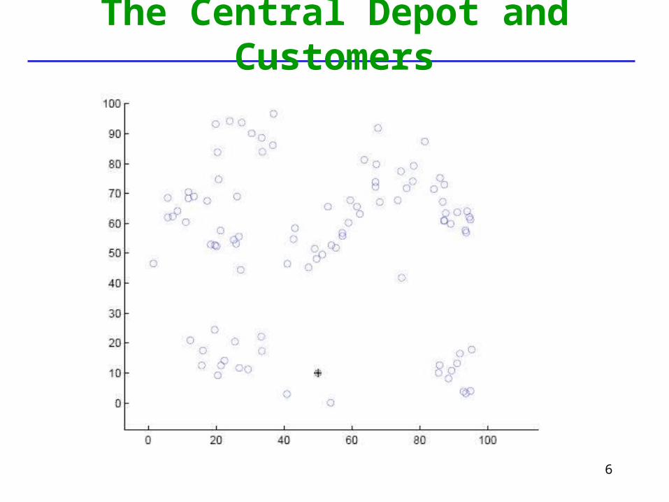
6

The Central Depot and Customers

7

Use Geometry to Find Supernodes

8

Solve the TSP

9

Reposition Supernodes and Solve Again

10

Computational Experiments

We focused on the location and relocation of the supernodes

Several heuristics were compared

Random and clustered data sets were tested

The number of customers and the radius were varied

The best heuristic seems to work well

In the real-world, meter reading takes place over a street network

11

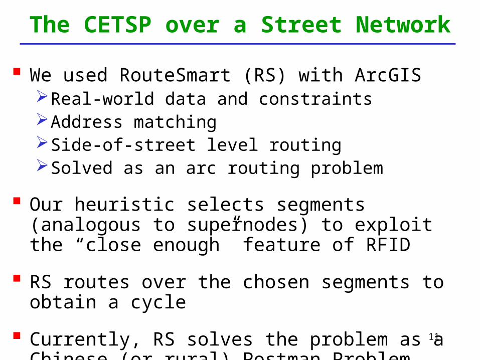
We used RouteSmart (RS) with ArcGISReal-world data and constraintsAddress matchingSide-of-street level routingSolved as an arc routing problem

Our heuristic selects segments (analogous to supernodes) to exploit the “close enough” feature of RFID

RS routes over the chosen segments to obtain a cycle

Currently, RS solves the problem as a Chinese (or rural) Postman Problem

The CETSP over a Street Network

12

How do we choose the street segments to feed into RS?

We tested several ideas

Two are simple greedy procedures

Greedy A: Choose the street segment that covers the most customers, remove those customers, and repeat until all customers are covered

Greedy B: Same as above, but order street segments based on the number of customers covered per unit length

Heuristic Implementation

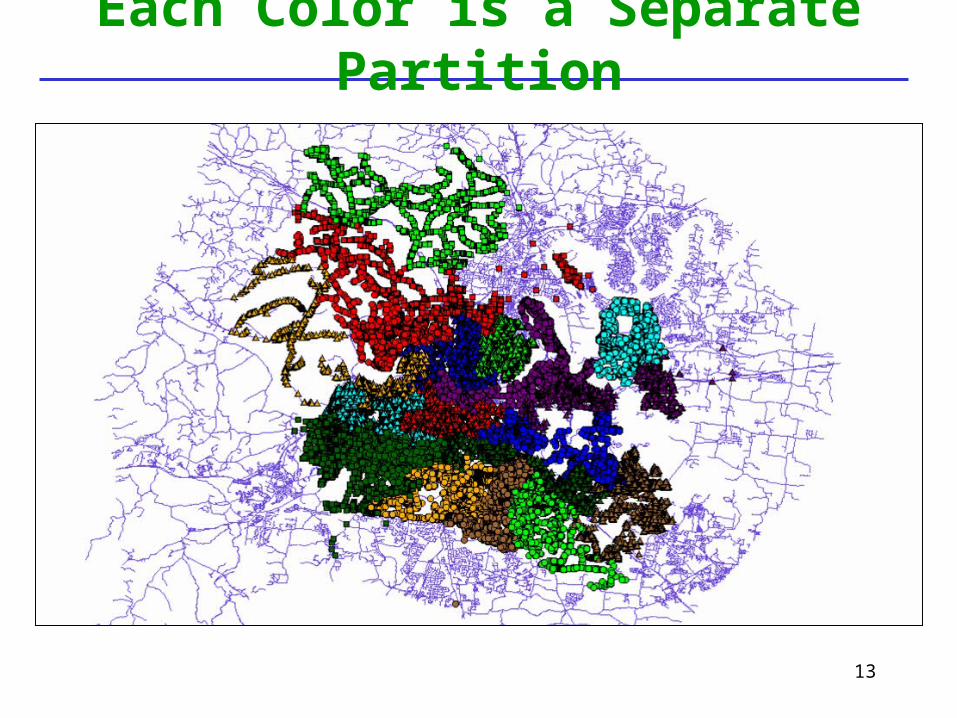
13

Each Color is a Separate Partition

14

A Single Partition

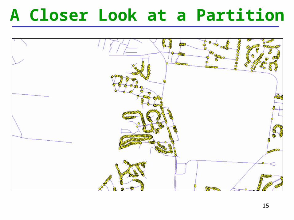
15

A Closer Look at a Partition

16

The Area Covered with RFID

17

The Area Covered by the Entire Partition

18

500 foot radius

Method Miles HoursNumber of Segments

Miles of Segments

Deadhead Miles

RS 204.8 9:22 1099 107.3 97.5

Greedy A 161.8 7:16 485 66.3 95.5

Greedy B 158.5 7:06 470 64.4 94.1

Essential − − 256 47.9 −

Some Preliminary Results

350 foot radius

RS 204.8 9:22 1099 107.3 97.5

Greedy A 171.9 7:45 621 78.1 93.8

Greedy B 171.2 7:43 610 78.0 93.2

Essential − − 451 67.9 −

19

The Colorful Traveling Salesman Problem

Given an undirected complete graph with colored edges as input

Each edge has a single color

Different edges can have the same color

Find a Hamiltonian tour with the minimum number of colors

This problem is related to the Minimum Label Spanning Tree problem

A hypothetical scenario follows

20

For his birthday, Michel wants to visit n cities without repetition and return home

All pairs of cities are directly connected by railroad or bus lines (edges)

There are l transport companies

Each company controls a subset of the edges

Each company charges the same monthly fee for using its edges

CTSP Motivation

21

CTSP Motivation - - continued

We can think of the edges owned by Company 1 as red, those owned by Company 2 as blue, and so on

The objective is to construct a Hamiltonian tour that uses the smallest number of colors

After much thought, Michel realizes that the CTSP is NP-complete since if he could solve the CTSP optimally, he could determine whether a graph has a Hamiltonian tour

He then solves the CTSP using his favorite metaheuristic and his birthday journey begins

Joyeux Anniversaire Michel!

22

Preliminary Results

We developed a path extension algorithm (PEA) and a genetic algorithm (GA) to solve the CTSP

We solved problems with 50, 100, 150, and 200 nodes and from 25 to 250 colors

Our experiments were run on a Pentium 4 PC with 1.80 GHz and 256 MB RAM

In general, GA outperforms PEA

Average running time for the GA on a graph with 200 nodes and 250 colors was 17.2 seconds

23

The Consistent Vehicle Routing Problem

This problem comes from a major package delivery company in the U.S.

Start with a capacitated vehicle routing problem (VRP)

Add two service quality constraintsEach customer must receive service from the same driver

each dayEach customer must receive service at roughly the same

time each day

24

The Consistent Vehicle Routing Problem

Assumptions

A week of service requirements is known in advanceAn unlimited number of vehicles each with fixed

capacity (or time limit) c

The Goal

Produce a set of routes for each day such that total weekly cost is minimized subject to the capacity and consistency constraints

25

A Simple Heuristic for the CVRP

Identify all customer locations requiring service on more than one day

Solve a capacitated VRP (capacity = (1 + λ) c) over these locations using sweep, savings, and 2-opt procedures

This results in a template of routes Create daily routes from the template

Remove customers who do not require service on that day

Insert all customers who require service only on that day

26

The Artificial Capacity

If we expect the daily routes to involve more insertions than removals from the template, then we set λ < 0

If we expect there to be more removals than insertions, then set λ > 0

In our experiments, we found that λ = 0.1 worked well

27

Implicit Rules that Guide the Heuristic

If customers i and j are on the same route on one day, then they must be on the same route every day both require service

If customer i is visited before customer j on one day, then this precedence must be satisfied every day both customers require service

Next, we examine how well these simple rules work

28

How Consistent are the Solutions?

The “same driver” requirement is automatically satisfied

The “same time” requirement is more complex Observation: The amount of service time variation

depends on the amount of customer overlap amongst the five daysLarge overlap → slight variationSmall overlap → increased variation

We performed several computational experiments

29

Experiment #1 Each customer requires service on each day with

equal probability p We varied p from 0.7 to 0.9 in steps of 0.02 Vehicle capacity is 500 minutes Vehicles travel one Euclidean unit of distance per

minute It takes one minute to service a customer There are k = 700 customers in total This results in about 100 to 125 customers per route Ten repetitions for each value of p

30

pMax Service

Time VariationMean Service

Time VariationMean Number

Customers/Route

Mean Number Vehicles

0.7 44.5 14.6 106.4 4.8

0.8 39.7 13.8 114.2 5.0

0.9 30.8 10.6 124.4 5.2

Service Time Variation

Bottom line: The level of consistency is quite high

31

Experiment #2 This experiment is of greater practical interest Here we have business customers and residential

customers Based on real-world data

70% are business customers30% are residential customersBusiness customers require service with probability 0.9

each dayResidential customers require service with probability

0.1 each day

We generated five data sets, each with 1000 customers

32

Data Set

Max Service Time Variation

Mean Service Time Variation

1 43.7 18.7

2 42.7 22.3

3 47.1 17.1

4 34.6 17.5

5 51.7 24.9

Avg. 44.0 20.1

Service Time Variation

Here, consistent service is important to business customers, not residential customers

33

The (Approximate) Cost of Consistency If we relax the consistency requirements, what would

the solutions look like? We looked at 10 homogeneous data sets with p = 0.7

and k = 800 On average, total cost is reduced by about 3.5% On the other hand, the mean service time variation

increases from 15 minutes to 3 hours We looked at 10 heterogeneous data sets also, and the

results were essentially the same Bottom line: The two simple rules ensure a high

degree of consistency

34

Conclusions

I have been working on vehicle routing problems since 1974

But, the area is as fresh and exciting to me NOW as it was when I began

Very interesting and practical new vehicle routing problems continue to emerge, as illustrated in this talk

I expect this to continue for quite some time Clever metaheuristics can often be used to obtain

excellent solutions to these new problems