1

A Review on Deep Learning TechniquesApplied to Semantic Segmentation

A. Garcia-Garcia, S. Orts-Escolano, S.O. Oprea, V. Villena-Martinez, and J. Garcia-Rodriguez

Abstract—Image semantic segmentation is more and more being of interest for computer vision and machine learning researchers.Many applications on the rise need accurate and efficient segmentation mechanisms: autonomous driving, indoor navigation, and evenvirtual or augmented reality systems to name a few. This demand coincides with the rise of deep learning approaches in almost everyfield or application target related to computer vision, including semantic segmentation or scene understanding. This paper provides areview on deep learning methods for semantic segmentation applied to various application areas. Firstly, we describe the terminologyof this field as well as mandatory background concepts. Next, the main datasets and challenges are exposed to help researchersdecide which are the ones that best suit their needs and their targets. Then, existing methods are reviewed, highlighting theircontributions and their significance in the field. Finally, quantitative results are given for the described methods and the datasets inwhich they were evaluated, following up with a discussion of the results. At last, we point out a set of promising future works and drawour own conclusions about the state of the art of semantic segmentation using deep learning techniques.

Index Terms—Semantic Segmentation, Deep Learning, Scene Labeling, Object Segmentation

F

1 INTRODUCTION

NOWADAYS, semantic segmentation – applied to still2D images, video, and even 3D or volumetric data

– is one of the key problems in the field of computervision. Looking at the big picture, semantic segmentationis one of the high-level task that paves the way towardscomplete scene understanding. The importance of sceneunderstanding as a core computer vision problem is high-lighted by the fact that an increasing number of applicationsnourish from inferring knowledge from imagery. Some ofthose applications include autonomous driving [1] [2] [3],human-machine interaction [4], computational photography[5], image search engines [6], and augmented reality to namea few. Such problem has been addressed in the past usingvarious traditional computer vision and machine learningtechniques. Despite the popularity of those kind of methods,the deep learning revolution has turned the tables so thatmany computer vision problems – semantic segmentationamong them – are being tackled using deep architectures,usually Convolutional Neural Networks (CNNs) [7] [8] [9][10] [11], which are surpassing other approaches by a largemargin in terms of accuracy and sometimes even efficiency.However, deep learning is far from the maturity achievedby other old-established branches of computer vision andmachine learning. Because of that, there is a lack of unifyingworks and state of the art reviews. The ever-changing stateof the field makes initiation difficult and keeping up withits evolution pace is an incredibly time-consuming task dueto the sheer amount of new literature being produced. Thismakes it hard to keep track of the works dealing with se-

• A. Garcia-Garcia, S.O. Oprea, V. Villena-Martinez, and J. Garcia-Rodriguez are with the Department of Computer Technology, Universityof Alicante, Spain.E-mail: {agarcia, soprea, vvillena, jgarcia}@dtic.ua.es

• S. Orts-Escolano is with the Department of Computer Science andArtificial Intelligence, Universit of Alicante, Spain.E-mail: sorts@ua.es.

mantic segmentation and properly interpret their proposals,prune subpar approaches, and validate results.

To the best of our knowledge, this is the first review tofocus explicitly on deep learning for semantic segmentation.Various semantic segmentation surveys already exist suchas the works by Zhu et al. [12] and Thoma [13], which doa great work summarizing and classifying existing meth-ods, discussing datasets and metrics, and providing designchoices for future research directions. However, they lacksome of the most recent datasets, they do not analyzeframeworks, and none of them provide details about deeplearning techniques. Because of that, we consider our workto be novel and helpful thus making it a significant contri-bution for the research community.

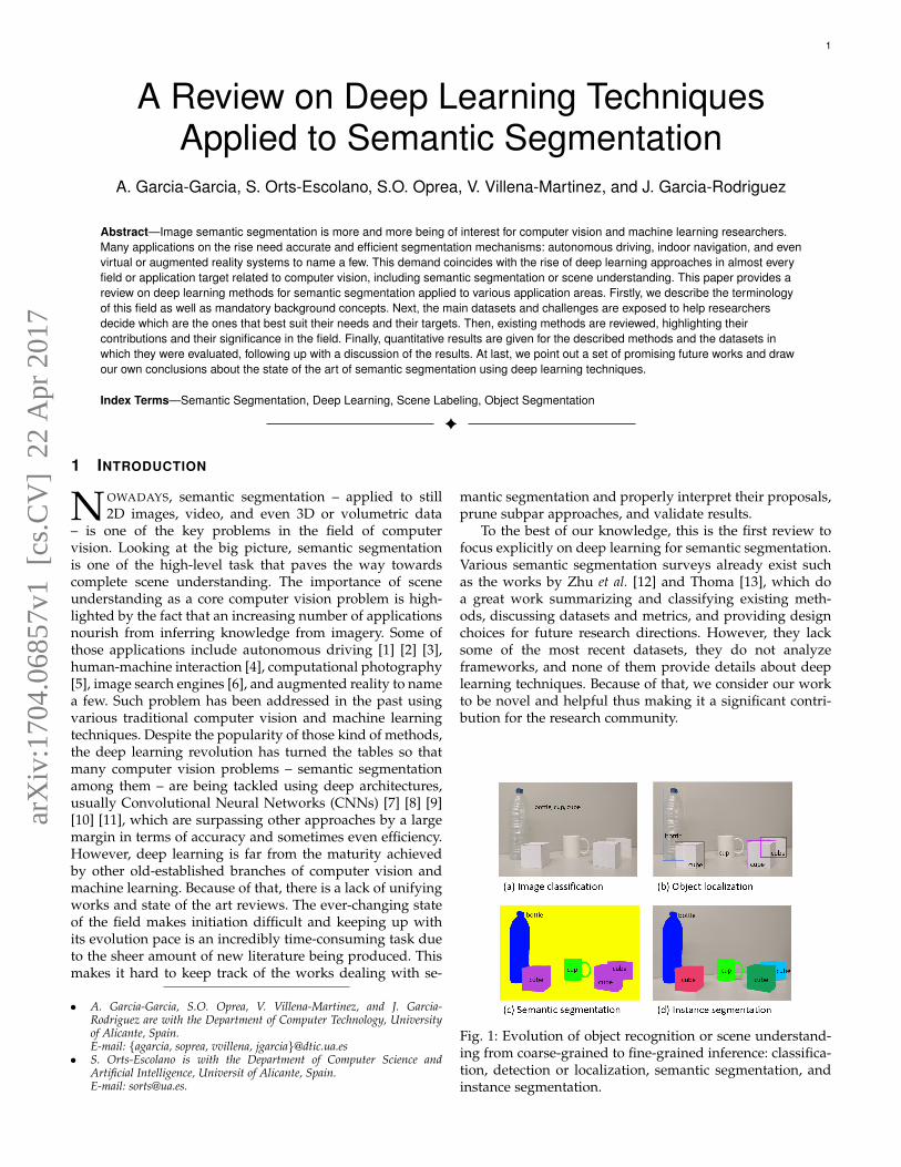
Fig. 1: Evolution of object recognition or scene understand-ing from coarse-grained to fine-grained inference: classifica-tion, detection or localization, semantic segmentation, andinstance segmentation.

arX

iv:1

704.

0685

7v1

[cs

.CV

] 2

2 A

pr 2

017

2

The key contributions of our work are as follows:

• We provide a broad survey of existing datasets thatmight be useful for segmentation projects with deeplearning techniques.

• An in-depth and organized review of the most sig-nificant methods that use deep learning for semanticsegmentation, their origins, and their contributions.

• A thorough performance evaluation which gathersquantitative metrics such as accuracy, execution time,and memory footprint.

• A discussion about the aforementioned results, aswell as a list of possible future works that might setthe course of upcoming advances, and a conclusionsummarizing the state of the art of the field.

The remainder of this paper is organized as follows.Firstly, Section 2 introduces the semantic segmentation prob-lem as well as notation and conventions commonly used inthe literature. Other background concepts such as commondeep neural networks are also reviewed. Next, Section 3describes existing datasets, challenges, and benchmarks.Section 4 reviews existing methods following a bottom-up complexity order based on their contributions. Thissection focuses on describing the theory and highlightsof those methods rather than performing a quantitativeevaluation. Finally, Section 5 presents a brief discussion onthe presented methods based on their quantitative resultson the aforementioned datasets. In addition, future researchdirections are also laid out. At last, Section 6 summarizesthe paper and draws conclusions about this work and thestate of the art of the field.

2 TERMINOLOGY AND BACKGROUND CONCEPTS

In order to properly understand how semantic segmenta-tion is tackled by modern deep learning architectures, it isimportant to know that it is not an isolated field but rather anatural step in the progression from coarse to fine inference.The origin could be located at classification, which consistsof making a prediction for a whole input, i.e., predictingwhich is the object in an image or even providing a rankedlist if there are many of them. Localization or detection is thenext step towards fine-grained inference, providing not onlythe classes but also additional information regarding thespatial location of those classes, e.g., centroids or boundingboxes. Providing that, it is obvious that semantic segmen-tation is the natural step to achieve fine-grained inference,its goal: make dense predictions inferring labels for everypixel; this way, each pixel is labeled with the class of its en-closing object or region. Further improvements can be made,such as instance segmentation (separate labels for differentinstances of the same class) and even part-based segmenta-tion (low-level decomposition of already segmented classesinto their components). Figure 1 shows the aforementionedevolution. In this review, we will mainly focus on genericscene labeling, i.e., per-pixel class segmentation, but we willalso review the most important methods on instance andpart-based segmentation.

In the end, the per-pixel labeling problem can be reducedto the following formulation: find a way to assign a statefrom the label space L = {l1, l2, ..., lk} to each one of the

elements of a set of random variables X = {x1, x2, ..., xN}.Each label l represents a different class or object, e.g., aero-plane, car, traffic sign, or background. This label space hask possible states which are usually extended to k + 1 andtreating l0 as background or a void class. Usually, X is a 2Dimage of W ×H = N pixels x. However, that set of randomvariables can be extended to any dimensionality such asvolumetric data or hyperspectral images.

Apart from the problem formulation, it is importantto remark some background concepts that might help thereader to understand this review. Firstly, common networks,approaches, and design decisions that are often used as thebasis for deep semantic segmentation systems. In addition,common techniques for training such as transfer learning.At last, data pre-processing and augmentation approaches.

2.1 Common Deep Network Architectures

As we previously stated, certain deep networks have madesuch significant contributions to the field that they havebecome widely known standards. It is the case of AlexNet,VGG-16, GoogLeNet, and ResNet. Such was their impor-tance that they are currently being used as building blocksfor many segmentation architectures. For that reason, wewill devote this section to review them.

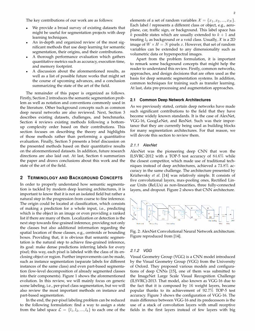
2.1.1 AlexNetAlexNet was the pioneering deep CNN that won theILSVRC-2012 with a TOP-5 test accuracy of 84.6% whilethe closest competitor, which made use of traditional tech-niques instead of deep architectures, achieved a 73.8% ac-curacy in the same challenge. The architecture presented byKrizhevsky et al. [14] was relatively simple. It consists offive convolutional layers, max-pooling ones, Rectified Lin-ear Units (ReLUs) as non-linearities, three fully-connectedlayers, and dropout. Figure 2 shows that CNN architecture.

Fig. 2: AlexNet Convolutional Neural Network architecture.Figure reproduced from [14].

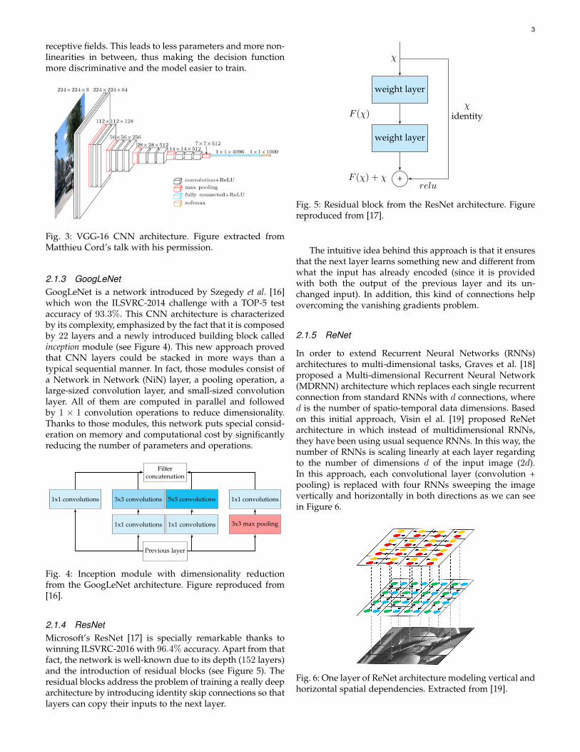
2.1.2 VGGVisual Geometry Group (VGG) is a CNN model introducedby the Visual Geometry Group (VGG) from the Universityof Oxford. They proposed various models and configura-tions of deep CNNs [15], one of them was submitted tothe ImageNet Large Scale Visual Recognition Challenge(ILSVRC)-2013. That model, also known as VGG-16 due tothe fact that it is composed by 16 weight layers, becamepopular thanks to its achievement of 92.7% TOP-5 testaccuracy. Figure 3 shows the configuration of VGG-16. Themain difference between VGG-16 and its predecessors is theuse of a stack of convolution layers with small receptivefields in the first layers instead of few layers with big

3

receptive fields. This leads to less parameters and more non-linearities in between, thus making the decision functionmore discriminative and the model easier to train.

Fig. 3: VGG-16 CNN architecture. Figure extracted fromMatthieu Cord’s talk with his permission.

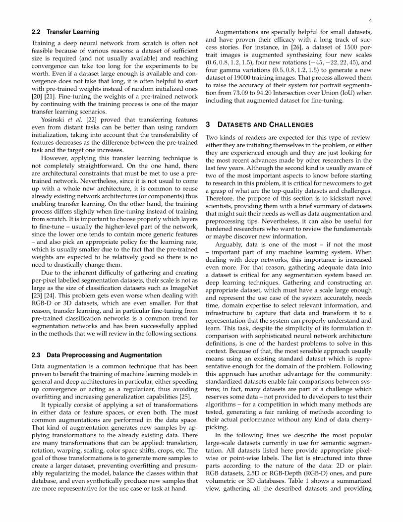
2.1.3 GoogLeNetGoogLeNet is a network introduced by Szegedy et al. [16]which won the ILSVRC-2014 challenge with a TOP-5 testaccuracy of 93.3%. This CNN architecture is characterizedby its complexity, emphasized by the fact that it is composedby 22 layers and a newly introduced building block calledinception module (see Figure 4). This new approach provedthat CNN layers could be stacked in more ways than atypical sequential manner. In fact, those modules consist ofa Network in Network (NiN) layer, a pooling operation, alarge-sized convolution layer, and small-sized convolutionlayer. All of them are computed in parallel and followedby 1 × 1 convolution operations to reduce dimensionality.Thanks to those modules, this network puts special consid-eration on memory and computational cost by significantlyreducing the number of parameters and operations.

Filterconcatenation

3x3 convolutions 5x5 convolutions1x1 convolutions 1x1 convolutions

1x1 convolutions 1x1 convolutions 3x3 max pooling

Previous layer

Fig. 4: Inception module with dimensionality reductionfrom the GoogLeNet architecture. Figure reproduced from[16].

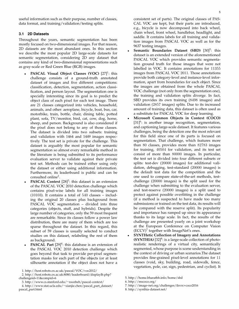
2.1.4 ResNetMicrosoft’s ResNet [17] is specially remarkable thanks towinning ILSVRC-2016 with 96.4% accuracy. Apart from thatfact, the network is well-known due to its depth (152 layers)and the introduction of residual blocks (see Figure 5). Theresidual blocks address the problem of training a really deeparchitecture by introducing identity skip connections so thatlayers can copy their inputs to the next layer.

weight layer

weight layer

+F (χ) + χ

χ

F (χ)χ

identity

relu

Fig. 5: Residual block from the ResNet architecture. Figurereproduced from [17].

The intuitive idea behind this approach is that it ensuresthat the next layer learns something new and different fromwhat the input has already encoded (since it is providedwith both the output of the previous layer and its un-changed input). In addition, this kind of connections helpovercoming the vanishing gradients problem.

2.1.5 ReNet

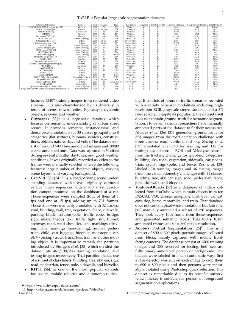
In order to extend Recurrent Neural Networks (RNNs)architectures to multi-dimensional tasks, Graves et al. [18]proposed a Multi-dimensional Recurrent Neural Network(MDRNN) architecture which replaces each single recurrentconnection from standard RNNs with d connections, whered is the number of spatio-temporal data dimensions. Basedon this initial approach, Visin el al. [19] proposed ReNetarchitecture in which instead of multidimensional RNNs,they have been using usual sequence RNNs. In this way, thenumber of RNNs is scaling linearly at each layer regardingto the number of dimensions d of the input image (2d).In this approach, each convolutional layer (convolution +pooling) is replaced with four RNNs sweeping the imagevertically and horizontally in both directions as we can seein Figure 6.

Fig. 6: One layer of ReNet architecture modeling vertical andhorizontal spatial dependencies. Extracted from [19].

4

2.2 Transfer Learning

Training a deep neural network from scratch is often notfeasible because of various reasons: a dataset of sufficientsize is required (and not usually available) and reachingconvergence can take too long for the experiments to beworth. Even if a dataset large enough is available and con-vergence does not take that long, it is often helpful to startwith pre-trained weights instead of random initialized ones[20] [21]. Fine-tuning the weights of a pre-trained networkby continuing with the training process is one of the majortransfer learning scenarios.

Yosinski et al. [22] proved that transferring featureseven from distant tasks can be better than using randominitialization, taking into account that the transferability offeatures decreases as the difference between the pre-trainedtask and the target one increases.

However, applying this transfer learning technique isnot completely straightforward. On the one hand, thereare architectural constraints that must be met to use a pre-trained network. Nevertheless, since it is not usual to comeup with a whole new architecture, it is common to reusealready existing network architectures (or components) thusenabling transfer learning. On the other hand, the trainingprocess differs slightly when fine-tuning instead of trainingfrom scratch. It is important to choose properly which layersto fine-tune – usually the higher-level part of the network,since the lower one tends to contain more generic features– and also pick an appropriate policy for the learning rate,which is usually smaller due to the fact that the pre-trainedweights are expected to be relatively good so there is noneed to drastically change them.

Due to the inherent difficulty of gathering and creatingper-pixel labelled segmentation datasets, their scale is not aslarge as the size of classification datasets such as ImageNet[23] [24]. This problem gets even worse when dealing withRGB-D or 3D datasets, which are even smaller. For thatreason, transfer learning, and in particular fine-tuning frompre-trained classification networks is a common trend forsegmentation networks and has been successfully appliedin the methods that we will review in the following sections.

2.3 Data Preprocessing and Augmentation

Data augmentation is a common technique that has beenproven to benefit the training of machine learning models ingeneral and deep architectures in particular; either speedingup convergence or acting as a regularizer, thus avoidingoverfitting and increasing generalization capabilities [25].

It typically consist of applying a set of transformationsin either data or feature spaces, or even both. The mostcommon augmentations are performed in the data space.That kind of augmentation generates new samples by ap-plying transformations to the already existing data. Thereare many transformations that can be applied: translation,rotation, warping, scaling, color space shifts, crops, etc. Thegoal of those transformations is to generate more samples tocreate a larger dataset, preventing overfitting and presum-ably regularizing the model, balance the classes within thatdatabase, and even synthetically produce new samples thatare more representative for the use case or task at hand.

Augmentations are specially helpful for small datasets,and have proven their efficacy with a long track of suc-cess stories. For instance, in [26], a dataset of 1500 por-trait images is augmented synthesizing four new scales(0.6, 0.8, 1.2, 1.5), four new rotations (−45,−22, 22, 45), andfour gamma variations (0.5, 0.8, 1.2, 1.5) to generate a newdataset of 19000 training images. That process allowed themto raise the accuracy of their system for portrait segmenta-tion from 73.09 to 94.20 Intersection over Union (IoU) whenincluding that augmented dataset for fine-tuning.

3 DATASETS AND CHALLENGES

Two kinds of readers are expected for this type of review:either they are initiating themselves in the problem, or eitherthey are experienced enough and they are just looking forthe most recent advances made by other researchers in thelast few years. Although the second kind is usually aware oftwo of the most important aspects to know before startingto research in this problem, it is critical for newcomers to geta grasp of what are the top-quality datasets and challenges.Therefore, the purpose of this section is to kickstart novelscientists, providing them with a brief summary of datasetsthat might suit their needs as well as data augmentation andpreprocessing tips. Nevertheless, it can also be useful forhardened researchers who want to review the fundamentalsor maybe discover new information.

Arguably, data is one of the most – if not the most– important part of any machine learning system. Whendealing with deep networks, this importance is increasedeven more. For that reason, gathering adequate data intoa dataset is critical for any segmentation system based ondeep learning techniques. Gathering and constructing anappropriate dataset, which must have a scale large enoughand represent the use case of the system accurately, needstime, domain expertise to select relevant information, andinfrastructure to capture that data and transform it to arepresentation that the system can properly understand andlearn. This task, despite the simplicity of its formulation incomparison with sophisticated neural network architecturedefinitions, is one of the hardest problems to solve in thiscontext. Because of that, the most sensible approach usuallymeans using an existing standard dataset which is repre-sentative enough for the domain of the problem. Followingthis approach has another advantage for the community:standardized datasets enable fair comparisons between sys-tems; in fact, many datasets are part of a challenge whichreserves some data – not provided to developers to test theiralgorithms – for a competition in which many methods aretested, generating a fair ranking of methods according totheir actual performance without any kind of data cherry-picking.

In the following lines we describe the most popularlarge-scale datasets currently in use for semantic segmen-tation. All datasets listed here provide appropriate pixel-wise or point-wise labels. The list is structured into threeparts according to the nature of the data: 2D or plainRGB datasets, 2.5D or RGB-Depth (RGB-D) ones, and purevolumetric or 3D databases. Table 1 shows a summarizedview, gathering all the described datasets and providing

5

useful information such as their purpose, number of classes,data format, and training/validation/testing splits.

3.1 2D DatasetsThroughout the years, semantic segmentation has beenmostly focused on two-dimensional images. For that reason,2D datasets are the most abundant ones. In this sectionwe describe the most popular 2D large-scale datasets forsemantic segmentation, considering 2D any dataset thatcontains any kind of two-dimensional representations suchas gray-scale or Red Green Blue (RGB) images.

• PASCAL Visual Object Classes (VOC) [27]1: thischallenge consists of a ground-truth annotateddataset of images and five different competitions:classification, detection, segmentation, action classi-fication, and person layout. The segmentation one isspecially interesting since its goal is to predict theobject class of each pixel for each test image. Thereare 21 classes categorized into vehicles, household,animals, and other: aeroplane, bicycle, boat, bus, car,motorbike, train, bottle, chair, dining table, pottedplant, sofa, TV/monitor, bird, cat, cow, dog, horse,sheep, and person. Background is also considered ifthe pixel does not belong to any of those classes.The dataset is divided into two subsets: trainingand validation with 1464 and 1449 images respec-tively. The test set is private for the challenge. Thisdataset is arguably the most popular for semanticsegmentation so almost every remarkable method inthe literature is being submitted to its performanceevaluation server to validate against their privatetest set. Methods can be trained either using onlythe dataset or either using additional information.Furthermore, its leaderboard is public and can beconsulted online2.

• PASCAL Context [28]3: this dataset is an extensionof the PASCAL VOC 2010 detection challenge whichcontains pixel-wise labels for all training images(10103). It contains a total of 540 classes – includ-ing the original 20 classes plus background fromPASCAL VOC segmentation – divided into threecategories (objects, stuff, and hybrids). Despite thelarge number of categories, only the 59 most frequentare remarkable. Since its classes follow a power lawdistribution, there are many of them which are toosparse throughout the dataset. In this regard, thissubset of 59 classes is usually selected to conductstudies on this dataset, relabeling the rest of themas background.

• PASCAL Part [29]4: this database is an extension ofthe PASCAL VOC 2010 detection challenge whichgoes beyond that task to provide per-pixel segmen-tation masks for each part of the objects (or at leastsilhouette annotation if the object does not have a

1. http://host.robots.ox.ac.uk/pascal/VOC/voc2012/2. http://host.robots.ox.ac.uk:8080/leaderboard/displaylb.php?

challengeid=11&compid=63. http://www.cs.stanford.edu/∼roozbeh/pascal-context/4. http://www.stat.ucla.edu/∼xianjie.chen/pascal part dataset/

pascal part.html

consistent set of parts). The original classes of PAS-CAL VOC are kept, but their parts are introduced,e.g., bicycle is now decomposed into back wheel,chain wheel, front wheel, handlebar, headlight, andsaddle. It contains labels for all training and valida-tion images from PASCAL VOC as well as for the9637 testing images.

• Semantic Boundaries Dataset (SBD) [30]5: thisdataset is an extended version of the aforementionedPASCAL VOC which provides semantic segmenta-tion ground truth for those images that were notlabelled in VOC. It contains annotations for 11355images from PASCAL VOC 2011. Those annotationsprovide both category-level and instance-level infor-mation, apart from boundaries for each object. Sincethe images are obtained from the whole PASCALVOC challenge (not only from the segmentation one),the training and validation splits diverge. In fact,SBD provides its own training (8498 images) andvalidation (2857 images) splits. Due to its increasedamount of training data, this dataset is often used asa substitute for PASCAL VOC for deep learning.

• Microsoft Common Objects in Context (COCO)[31]6: is another image recognition, segmentation,and captioning large-scale dataset. It features variouschallenges, being the detection one the most relevantfor this field since one of its parts is focused onsegmentation. That challenge, which features morethan 80 classes, provides more than 82783 imagesfor training, 40504 for validation, and its test setconsist of more than 80000 images. In particular,the test set is divided into four different subsets orsplits: test-dev (20000 images) for additional vali-dation, debugging, test-standard (20000 images) isthe default test data for the competition and theone used to compare state-of-the-art methods, test-challenge (20000 images) is the split used for thechallenge when submitting to the evaluation server,and test-reserve (20000 images) is a split used toprotect against possible overfitting in the challenge(if a method is suspected to have made too manysubmissions or trained on the test data, its results willbe compared with the reserve split). Its popularityand importance has ramped up since its appearancethanks to its large scale. In fact, the results of thechallenge are presented yearly on a joint workshopat the European Conference on Computer Vision(ECCV)7 together with ImageNet’s ones.

• SYNTHetic Collection of Imagery and Annotations(SYNTHIA) [32]8: is a large-scale collection of photo-realistic renderings of a virtual city, semanticallysegmented, whose purpose is scene understanding inthe context of driving or urban scenarios.The datasetprovides fine-grained pixel-level annotations for 11classes (void, sky, building, road, sidewalk, fence,vegetation, pole, car, sign, pedestrian, and cyclist). It

5. http://home.bharathh.info/home/sbd6. http://mscoco.org/7. http://image-net.org/challenges/ilsvrc+coco20168. http://synthia-dataset.net/

6

TABLE 1: Popular large-scale segmentation datasets.

Name and Reference Purpose Year Classes Data Resolution Sequence Synthetic/Real Samples (training) Samples (validation) Samples (test)PASCAL VOC 2012 Segmentation [27] Generic 2012 21 2D Variable 7 R 1464 1449 Private

PASCAL-Context [28] Generic 2014 540 (59) 2D Variable 7 R 10103 N/A 9637PASCAL-Part [29] Generic-Part 2014 20 2D Variable 7 R 10103 N/A 9637

SBD [30] Generic 2011 21 2D Variable 7 R 8498 2857 N/AMicrosoft COCO [31] Generic 2014 +80 2D Variable 7 R 82783 40504 81434

SYNTHIA [32] Urban (Driving) 2016 11 2D 960× 720 7 S 13407 N/A N/ACityscapes (fine) [33] Urban 2015 30 (8) 2D 2048× 1024 3 R 2975 500 1525

Cityscapes (coarse) [33] Urban 2015 30 (8) 2D 2048× 1024 3 R 22973 500 N/ACamVid [34] Urban (Driving) 2009 32 2D 960× 720 3 R 701 N/A N/A

CamVid-Sturgess [35] Urban (Driving) 2009 11 2D 960× 720 3 R 367 100 233KITTI-Layout [36] [37] Urban/Driving 2012 3 2D Variable 7 R 323 N/A N/A

KITTI-Ros [38] Urban/Driving 2015 11 2D Variable 7 R 170 N/A 46KITTI-Zhang [39] Urban/Driving 2015 10 2D/3D 1226× 370 7 R 140 N/A 112

Stanford background [40] Outdoor 2009 8 2D 320× 240 7 R 725 N/A N/ASiftFlow [41] Outdoor 2011 33 2D 256× 256 7 R 2688 N/A N/A

Youtube-Objects-Jain [42] Objects 2014 10 2D 480× 360 3 R 10167 N/A N/AAdobe’s Portrait Segmentation [26] Portrait 2016 2 2D 600× 800 7 R 1500 300 N/A

MINC [43] Materials 2015 23 2D Variable 7 R 7061 2500 5000DAVIS [44] [45] Generic 2016 4 2D 480p 3 R 4219 2023 2180NYUDv2 [46] Indoor 2012 40 2.5D 480× 640 7 R 795 654 N/ASUN3D [47] Indoor 2013 – 2.5D 640× 480 3 R 19640 N/A N/A

SUNRGBD [48] Indoor 2015 37 2.5D Variable 7 R 2666 2619 5050RGB-D Object Dataset [49] Household objects 2011 51 2.5D 640× 480 3 R 207920 N/A N/A

ShapeNet Part [50] Object/Part 2016 16/50 3D N/A 7 S 31, 963 N/A N/AStanford 2D-3D-S [51] Indoor 2017 13 2D/2.5D/3D 1080× 1080 3 R 70469 N/A N/A

3D Mesh [52] Object/Part 2009 19 3D N/A 7 S 380 N/A N/ASydney Urban Objects Dataset [53] Urban (Objects) 2013 26 3D N/A 7 R 41 N/A N/A

Large-Scale Point Cloud Classification Benchmark [54] Urban/Nature 2016 8 3D N/A 7 R 15 N/A 15

features 13407 training images from rendered videostreams. It is also characterized by its diversity interms of scenes (towns, cities, highways), dynamicobjects, seasons, and weather.

• Cityscapes [33]9: is a large-scale database whichfocuses on semantic understanding of urban streetscenes. It provides semantic, instance-wise, anddense pixel annotations for 30 classes grouped into 8categories (flat surfaces, humans, vehicles, construc-tions, objects, nature, sky, and void). The dataset con-sist of around 5000 fine annotated images and 20000coarse annotated ones. Data was captured in 50 citiesduring several months, daytimes, and good weatherconditions. It was originally recorded as video so theframes were manually selected to have the followingfeatures: large number of dynamic objects, varyingscene layout, and varying background.

• CamVid [55] [34]10: is a road/driving scene under-standing database which was originally capturedas five video sequences with a 960 × 720 resolu-tion camera mounted on the dashboard of a car.Those sequences were sampled (four of them at 1fps and one at 15 fps) adding up to 701 frames.Those stills were manually annotated with 32 classes:void, building, wall, tree, vegetation, fence, sidewalk,parking block, column/pole, traffic cone, bridge,sign, miscellaneous text, traffic light, sky, tunnel,archway, road, road shoulder, lane markings (driv-ing), lane markings (non-driving), animal, pedes-trian, child, cart luggage, bicyclist, motorcycle, car,SUV/pickup/truck, truck/bus, train, and other mov-ing object. It is important to remark the partitionintroduced by Sturgess et al. [35] which divided thedataset into 367/100/233 training, validation, andtesting images respectively. That partition makes useof a subset of class labels: building, tree, sky, car, sign,road, pedestrian, fence, pole, sidewalk, and bicyclist.

• KITTI [56]: is one of the most popular datasetsfor use in mobile robotics and autonomous driv-

9. https://www.cityscapes-dataset.com/10. http://mi.eng.cam.ac.uk/research/projects/VideoRec/

CamVid/

ing. It consists of hours of traffic scenarios recordedwith a variety of sensor modalities, including high-resolution RGB, grayscale stereo cameras, and a 3Dlaser scanner. Despite its popularity, the dataset itselfdoes not contain ground truth for semantic segmen-tation. However, various researchers have manuallyannotated parts of the dataset to fit their necessities.Alvarez et al. [36] [37] generated ground truth for323 images from the road detection challenge withthree classes: road, vertical, and sky. Zhang et al.[39] annotated 252 (140 for training and 112 fortesting) acquisitions – RGB and Velodyne scans –from the tracking challenge for ten object categories:building, sky, road, vegetation, sidewalk, car, pedes-trian, cyclist, sign/pole, and fence. Ros et al. [38]labeled 170 training images and 46 testing images(from the visual odometry challenge) with 11 classes:building, tree, sky, car, sign, road, pedestrian, fence,pole, sidewalk, and bicyclist.

• Youtube-Objects [57] is a database of videos col-lected from YouTube which contain objects from tenPASCAL VOC classes: aeroplane, bird, boat, car, cat,cow, dog, horse, motorbike, and train. That databasedoes not contain pixel-wise annotations but Jain et al.[42] manually annotated a subset of 126 sequences.They took every 10th frame from those sequencesand generated semantic labels. That totals 10167annotated frames at 480× 360 pixels resolution.

• Adobe’s Portrait Segmentation [26]11: this is adataset of 800 × 600 pixels portrait images collectedfrom Flickr, mainly captured with mobile front-facing cameras. The database consist of 1500 trainingimages and 300 reserved for testing, both sets arefully binary annotated: person or background. Theimages were labeled in a semi-automatic way: firsta face detector was run on each image to crop themto 600 × 800 pixels and then persons were manu-ally annotated using Photoshop quick selection. Thisdataset is remarkable due to its specific purposewhich makes it suitable for person in foregroundsegmentation applications.

11. http://xiaoyongshen.me/webpage portrait/index.html

7

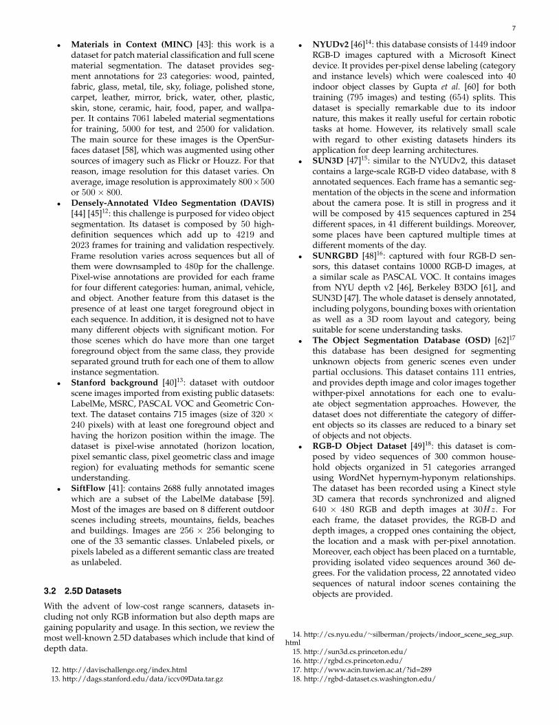
• Materials in Context (MINC) [43]: this work is adataset for patch material classification and full scenematerial segmentation. The dataset provides seg-ment annotations for 23 categories: wood, painted,fabric, glass, metal, tile, sky, foliage, polished stone,carpet, leather, mirror, brick, water, other, plastic,skin, stone, ceramic, hair, food, paper, and wallpa-per. It contains 7061 labeled material segmentationsfor training, 5000 for test, and 2500 for validation.The main source for these images is the OpenSur-faces dataset [58], which was augmented using othersources of imagery such as Flickr or Houzz. For thatreason, image resolution for this dataset varies. Onaverage, image resolution is approximately 800×500or 500× 800.

• Densely-Annotated VIdeo Segmentation (DAVIS)[44] [45]12: this challenge is purposed for video objectsegmentation. Its dataset is composed by 50 high-definition sequences which add up to 4219 and2023 frames for training and validation respectively.Frame resolution varies across sequences but all ofthem were downsampled to 480p for the challenge.Pixel-wise annotations are provided for each framefor four different categories: human, animal, vehicle,and object. Another feature from this dataset is thepresence of at least one target foreground object ineach sequence. In addition, it is designed not to havemany different objects with significant motion. Forthose scenes which do have more than one targetforeground object from the same class, they provideseparated ground truth for each one of them to allowinstance segmentation.

• Stanford background [40]13: dataset with outdoorscene images imported from existing public datasets:LabelMe, MSRC, PASCAL VOC and Geometric Con-text. The dataset contains 715 images (size of 320 ×240 pixels) with at least one foreground object andhaving the horizon position within the image. Thedataset is pixel-wise annotated (horizon location,pixel semantic class, pixel geometric class and imageregion) for evaluating methods for semantic sceneunderstanding.

• SiftFlow [41]: contains 2688 fully annotated imageswhich are a subset of the LabelMe database [59].Most of the images are based on 8 different outdoorscenes including streets, mountains, fields, beachesand buildings. Images are 256 × 256 belonging toone of the 33 semantic classes. Unlabeled pixels, orpixels labeled as a different semantic class are treatedas unlabeled.

3.2 2.5D Datasets

With the advent of low-cost range scanners, datasets in-cluding not only RGB information but also depth maps aregaining popularity and usage. In this section, we review themost well-known 2.5D databases which include that kind ofdepth data.

12. http://davischallenge.org/index.html13. http://dags.stanford.edu/data/iccv09Data.tar.gz

• NYUDv2 [46]14: this database consists of 1449 indoorRGB-D images captured with a Microsoft Kinectdevice. It provides per-pixel dense labeling (categoryand instance levels) which were coalesced into 40indoor object classes by Gupta et al. [60] for bothtraining (795 images) and testing (654) splits. Thisdataset is specially remarkable due to its indoornature, this makes it really useful for certain robotictasks at home. However, its relatively small scalewith regard to other existing datasets hinders itsapplication for deep learning architectures.

• SUN3D [47]15: similar to the NYUDv2, this datasetcontains a large-scale RGB-D video database, with 8annotated sequences. Each frame has a semantic seg-mentation of the objects in the scene and informationabout the camera pose. It is still in progress and itwill be composed by 415 sequences captured in 254different spaces, in 41 different buildings. Moreover,some places have been captured multiple times atdifferent moments of the day.

• SUNRGBD [48]16: captured with four RGB-D sen-sors, this dataset contains 10000 RGB-D images, ata similar scale as PASCAL VOC. It contains imagesfrom NYU depth v2 [46], Berkeley B3DO [61], andSUN3D [47]. The whole dataset is densely annotated,including polygons, bounding boxes with orientationas well as a 3D room layout and category, beingsuitable for scene understanding tasks.

• The Object Segmentation Database (OSD) [62]17

this database has been designed for segmentingunknown objects from generic scenes even underpartial occlusions. This dataset contains 111 entries,and provides depth image and color images togetherwithper-pixel annotations for each one to evalu-ate object segmentation approaches. However, thedataset does not differentiate the category of differ-ent objects so its classes are reduced to a binary setof objects and not objects.

• RGB-D Object Dataset [49]18: this dataset is com-posed by video sequences of 300 common house-hold objects organized in 51 categories arrangedusing WordNet hypernym-hyponym relationships.The dataset has been recorded using a Kinect style3D camera that records synchronized and aligned640 × 480 RGB and depth images at 30Hz. Foreach frame, the dataset provides, the RGB-D anddepth images, a cropped ones containing the object,the location and a mask with per-pixel annotation.Moreover, each object has been placed on a turntable,providing isolated video sequences around 360 de-grees. For the validation process, 22 annotated videosequences of natural indoor scenes containing theobjects are provided.

14. http://cs.nyu.edu/∼silberman/projects/indoor scene seg sup.html

15. http://sun3d.cs.princeton.edu/16. http://rgbd.cs.princeton.edu/17. http://www.acin.tuwien.ac.at/?id=28918. http://rgbd-dataset.cs.washington.edu/

8

3.3 3D Datasets

Pure three-dimensional databases are scarce, this kind ofdatasets usually provide Computer Aided Design (CAD)meshes or other volumetric representations, such as pointclouds. Generating large-scale 3D datasets for segmentationis costly and difficult, and not many deep learning methodsare able to process that kind of data as it is. For thosereasons, 3D datasets are not quite popular at the moment. Inspite of that fact, we describe the most promising ones forthe task at hand.

• ShapeNet Part [50]19: is a subset of the ShapeNet [63]repository which focuses on fine-grained 3D objectsegmentation. It contains 31, 693 meshes sampledfrom 16 categories of the original dataset (airplane,earphone, cap, motorbike, bag, mug, laptop, table,guitar, knife, rocket, lamp, chair, pistol, car, andskateboard). Each shape class is labeled with two tofive parts (totalling 50 object parts across the wholedataset), e.g., each shape from the airplane class islabeled with wings, body, tail, and engine. Ground-truth labels are provided on points sampled from themeshes.

• Stanford 2D-3D-S [51]20: is a multi-modal and large-scale indoor spaces dataset extending the Stanford3D Semantic Parsing work [64]. It provides a va-riety of registered modalities – 2D (RGB), 2.5D(depth maps and surface normals), and 3D (meshesand point clouds) – with semantic annotations. Thedatabase is composed of 70, 496 full high-definitionRGB images (1080×1080 resolution) along with theircorresponding depth maps, surface normals, meshes,and point clouds with semantic annotations (per-pixel and per-point). That data were captured in sixindoor areas from three different educational andoffice buildings. That makes a total of 271 rooms andapproximately 700 million points annotated withlabels from 13 categories: ceiling, floor, wall, column,beam, window, door, table, chair, bookcase, sofa,board, and clutter.

• A Benchmark for 3D Mesh Segmentation [52]21:this benchmark is composed by 380 meshes classifiedin 19 categories (human, cup, glasses, airplane, ant,chair, octopus, table, teddy, hand, plier, fish, bird,armadillo, bust, mech, bearing, vase, fourleg). Eachmesh has been manually segmented into functionalparts, the main goal is to provide a sample distribu-tion over ”how humans decompose each mesh intofunctional parts”.

• Sydney Urban Objects Dataset [53]22: this datasetcontains a variety of common urban road objectsscanned with a Velodyne HDK-64E LIDAR. There are631 individual scans (point clouds) of objects acrossclasses of vehicles, pedestrians, signs and trees. Theinteresting point of this dataset is that, for each

19. http://cs.stanford.edu/∼ericyi/project page/part annotation/20. http://buildingparser.stanford.edu21. http://segeval.cs.princeton.edu/22. http://www.acfr.usyd.edu.au/papers/

SydneyUrbanObjectsDataset.shtml

object, apart from the individual scan, a full 360-degrees annotated scan is provided.

• Large-Scale Point Cloud Classification Benchmark[54]23: this benchmark provides manually annotated3D point clouds of diverse natural and urban scenes:churches, streets, railroad tracks, squares, villages,soccer fields, castles among others. This dataset fea-tures statically captured point clouds with very finedetails and density. It contains 15 large-scale pointclouds for training and another 15 for testing. Itsscale can be grasped by the fact that it totals morethan one billion labelled points.

4 METHODS

The relentless success of deep learning techniques in varioushigh-level computer vision tasks – in particular, super-vised approaches such as Convolutional Neural Networks(CNNs) for image classification or object detection [14][15] [16] – motivated researchers to explore the capabilitiesof such networks for pixel-level labelling problems likesemantic segmentation. The key advantage of these deeplearning techniques, which gives them an edge over tradi-tional methods, is the ability to learn appropriate featurerepresentations for the problem at hand, e.g., pixel labellingon a particular dataset, in an end-to-end fashion instead ofusing hand-crafted features that require domain expertise,effort, and often too much fine-tuning to make them workon a particular scenario.

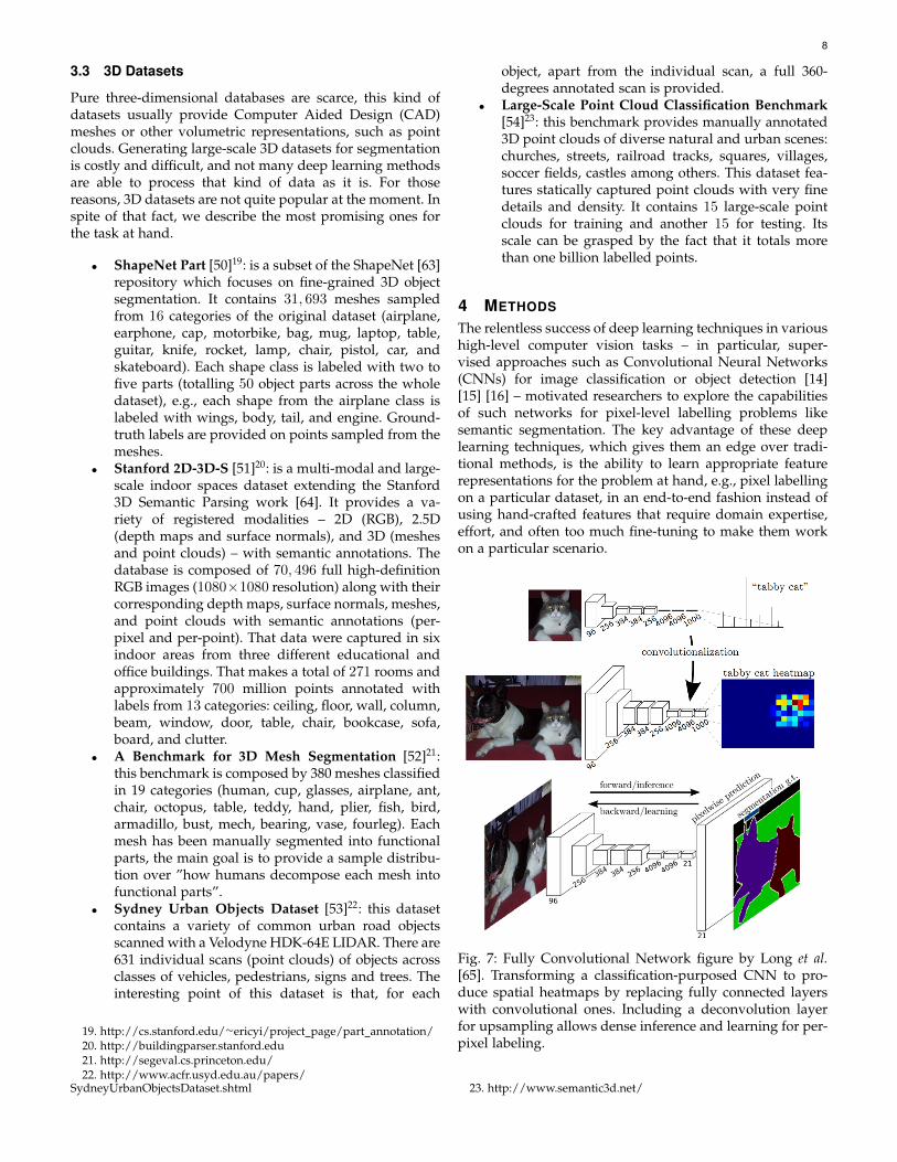
Fig. 7: Fully Convolutional Network figure by Long et al.[65]. Transforming a classification-purposed CNN to pro-duce spatial heatmaps by replacing fully connected layerswith convolutional ones. Including a deconvolution layerfor upsampling allows dense inference and learning for per-pixel labeling.

23. http://www.semantic3d.net/

9

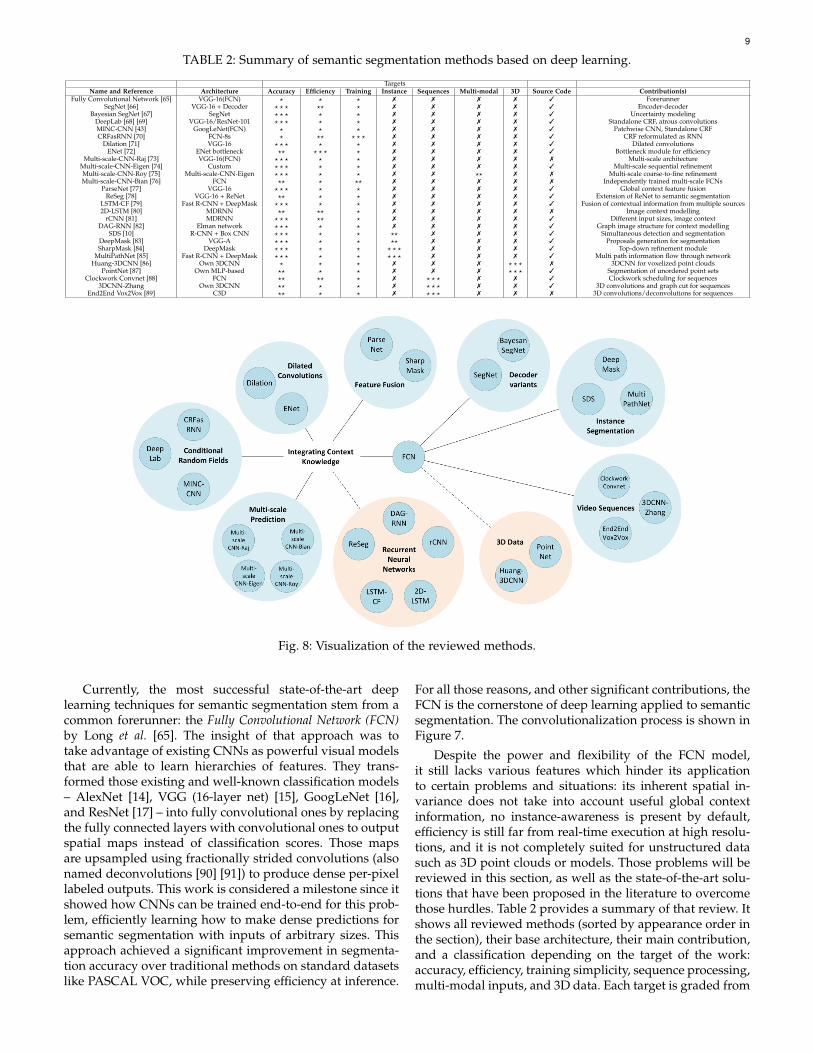
TABLE 2: Summary of semantic segmentation methods based on deep learning.

TargetsName and Reference Architecture Accuracy Efficiency Training Instance Sequences Multi-modal 3D Source Code Contribution(s)

Fully Convolutional Network [65] VGG-16(FCN) ? ? ? 7 7 7 7 3 ForerunnerSegNet [66] VGG-16 + Decoder ? ? ? ?? ? 7 7 7 7 3 Encoder-decoder

Bayesian SegNet [67] SegNet ? ? ? ? ? 7 7 7 7 3 Uncertainty modelingDeepLab [68] [69] VGG-16/ResNet-101 ? ? ? ? ? 7 7 7 7 3 Standalone CRF, atrous convolutionsMINC-CNN [43] GoogLeNet(FCN) ? ? ? 7 7 7 7 3 Patchwise CNN, Standalone CRFCRFasRNN [70] FCN-8s ? ?? ? ? ? 7 7 7 7 3 CRF reformulated as RNN

Dilation [71] VGG-16 ? ? ? ? ? 7 7 7 7 3 Dilated convolutionsENet [72] ENet bottleneck ?? ? ? ? ? 7 7 7 7 3 Bottleneck module for efficiency

Multi-scale-CNN-Raj [73] VGG-16(FCN) ? ? ? ? ? 7 7 7 7 7 Multi-scale architectureMulti-scale-CNN-Eigen [74] Custom ? ? ? ? ? 7 7 7 7 3 Multi-scale sequential refinementMulti-scale-CNN-Roy [75] Multi-scale-CNN-Eigen ? ? ? ? ? 7 7 ?? 7 7 Multi-scale coarse-to-fine refinementMulti-scale-CNN-Bian [76] FCN ?? ? ?? 7 7 7 7 7 Independently trained multi-scale FCNs

ParseNet [77] VGG-16 ? ? ? ? ? 7 7 7 7 3 Global context feature fusionReSeg [78] VGG-16 + ReNet ?? ? ? 7 7 7 7 3 Extension of ReNet to semantic segmentation

LSTM-CF [79] Fast R-CNN + DeepMask ? ? ? ? ? 7 7 7 7 3 Fusion of contextual information from multiple sources2D-LSTM [80] MDRNN ?? ?? ? 7 7 7 7 7 Image context modelling

rCNN [81] MDRNN ? ? ? ?? ? 7 7 7 7 3 Different input sizes, image contextDAG-RNN [82] Elman network ? ? ? ? ? 7 7 7 7 3 Graph image structure for context modelling

SDS [10] R-CNN + Box CNN ? ? ? ? ? ?? 7 7 7 3 Simultaneous detection and segmentationDeepMask [83] VGG-A ? ? ? ? ? ?? 7 7 7 3 Proposals generation for segmentationSharpMask [84] DeepMask ? ? ? ? ? ? ? ? 7 7 7 3 Top-down refinement module

MultiPathNet [85] Fast R-CNN + DeepMask ? ? ? ? ? ? ? ? 7 7 7 3 Multi path information flow through networkHuang-3DCNN [86] Own 3DCNN ? ? ? 7 7 7 ? ? ? 7 3DCNN for voxelized point clouds

PointNet [87] Own MLP-based ?? ? ? 7 7 7 ? ? ? 3 Segmentation of unordered point setsClockwork Convnet [88] FCN ?? ?? ? 7 ? ? ? 7 7 3 Clockwork scheduling for sequences

3DCNN-Zhang Own 3DCNN ?? ? ? 7 ? ? ? 7 7 3 3D convolutions and graph cut for sequencesEnd2End Vox2Vox [89] C3D ?? ? ? 7 ? ? ? 7 7 7 3D convolutions/deconvolutions for sequences

Fig. 8: Visualization of the reviewed methods.

Currently, the most successful state-of-the-art deeplearning techniques for semantic segmentation stem from acommon forerunner: the Fully Convolutional Network (FCN)by Long et al. [65]. The insight of that approach was totake advantage of existing CNNs as powerful visual modelsthat are able to learn hierarchies of features. They trans-formed those existing and well-known classification models– AlexNet [14], VGG (16-layer net) [15], GoogLeNet [16],and ResNet [17] – into fully convolutional ones by replacingthe fully connected layers with convolutional ones to outputspatial maps instead of classification scores. Those mapsare upsampled using fractionally strided convolutions (alsonamed deconvolutions [90] [91]) to produce dense per-pixellabeled outputs. This work is considered a milestone since itshowed how CNNs can be trained end-to-end for this prob-lem, efficiently learning how to make dense predictions forsemantic segmentation with inputs of arbitrary sizes. Thisapproach achieved a significant improvement in segmenta-tion accuracy over traditional methods on standard datasetslike PASCAL VOC, while preserving efficiency at inference.

For all those reasons, and other significant contributions, theFCN is the cornerstone of deep learning applied to semanticsegmentation. The convolutionalization process is shown inFigure 7.

Despite the power and flexibility of the FCN model,it still lacks various features which hinder its applicationto certain problems and situations: its inherent spatial in-variance does not take into account useful global contextinformation, no instance-awareness is present by default,efficiency is still far from real-time execution at high resolu-tions, and it is not completely suited for unstructured datasuch as 3D point clouds or models. Those problems will bereviewed in this section, as well as the state-of-the-art solu-tions that have been proposed in the literature to overcomethose hurdles. Table 2 provides a summary of that review. Itshows all reviewed methods (sorted by appearance order inthe section), their base architecture, their main contribution,and a classification depending on the target of the work:accuracy, efficiency, training simplicity, sequence processing,multi-modal inputs, and 3D data. Each target is graded from

10

one to three stars (?) depending on how much focus puts thework on it, and a mark (7) if that issue is not addressed. Inaddition, Figure 8 shows a graph of the reviewed methodsfor the sake of visualization.

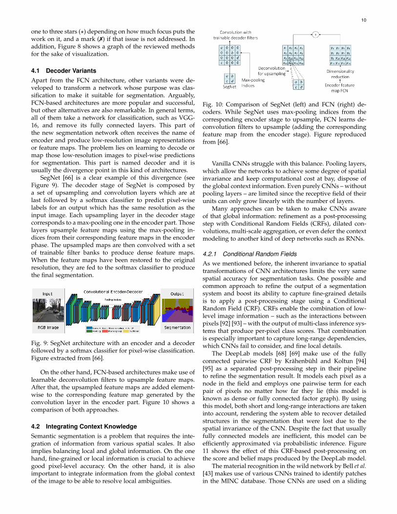
4.1 Decoder VariantsApart from the FCN architecture, other variants were de-veloped to transform a network whose purpose was clas-sification to make it suitable for segmentation. Arguably,FCN-based architectures are more popular and successful,but other alternatives are also remarkable. In general terms,all of them take a network for classification, such as VGG-16, and remove its fully connected layers. This part ofthe new segmentation network often receives the name ofencoder and produce low-resolution image representationsor feature maps. The problem lies on learning to decode ormap those low-resolution images to pixel-wise predictionsfor segmentation. This part is named decoder and it isusually the divergence point in this kind of architectures.

SegNet [66] is a clear example of this divergence (seeFigure 9). The decoder stage of SegNet is composed bya set of upsampling and convolution layers which are atlast followed by a softmax classifier to predict pixel-wiselabels for an output which has the same resolution as theinput image. Each upsampling layer in the decoder stagecorresponds to a max-pooling one in the encoder part. Thoselayers upsample feature maps using the max-pooling in-dices from their corresponding feature maps in the encoderphase. The upsampled maps are then convolved with a setof trainable filter banks to produce dense feature maps.When the feature maps have been restored to the originalresolution, they are fed to the softmax classifier to producethe final segmentation.

Fig. 9: SegNet architecture with an encoder and a decoderfollowed by a softmax classifier for pixel-wise classification.Figure extracted from [66].

On the other hand, FCN-based architectures make use oflearnable deconvolution filters to upsample feature maps.After that, the upsampled feature maps are added element-wise to the corresponding feature map generated by theconvolution layer in the encoder part. Figure 10 shows acomparison of both approaches.

4.2 Integrating Context KnowledgeSemantic segmentation is a problem that requires the inte-gration of information from various spatial scales. It alsoimplies balancing local and global information. On the onehand, fine-grained or local information is crucial to achievegood pixel-level accuracy. On the other hand, it is alsoimportant to integrate information from the global contextof the image to be able to resolve local ambiguities.

Fig. 10: Comparison of SegNet (left) and FCN (right) de-coders. While SegNet uses max-pooling indices from thecorresponding encoder stage to upsample, FCN learns de-convolution filters to upsample (adding the correspondingfeature map from the encoder stage). Figure reproducedfrom [66].

Vanilla CNNs struggle with this balance. Pooling layers,which allow the networks to achieve some degree of spatialinvariance and keep computational cost at bay, dispose ofthe global context information. Even purely CNNs – withoutpooling layers – are limited since the receptive field of theirunits can only grow linearly with the number of layers.

Many approaches can be taken to make CNNs awareof that global information: refinement as a post-processingstep with Conditional Random Fields (CRFs), dilated con-volutions, multi-scale aggregation, or even defer the contextmodeling to another kind of deep networks such as RNNs.

4.2.1 Conditional Random FieldsAs we mentioned before, the inherent invariance to spatialtransformations of CNN architectures limits the very samespatial accuracy for segmentation tasks. One possible andcommon approach to refine the output of a segmentationsystem and boost its ability to capture fine-grained detailsis to apply a post-processing stage using a ConditionalRandom Field (CRF). CRFs enable the combination of low-level image information – such as the interactions betweenpixels [92] [93] – with the output of multi-class inference sys-tems that produce per-pixel class scores. That combinationis especially important to capture long-range dependencies,which CNNs fail to consider, and fine local details.

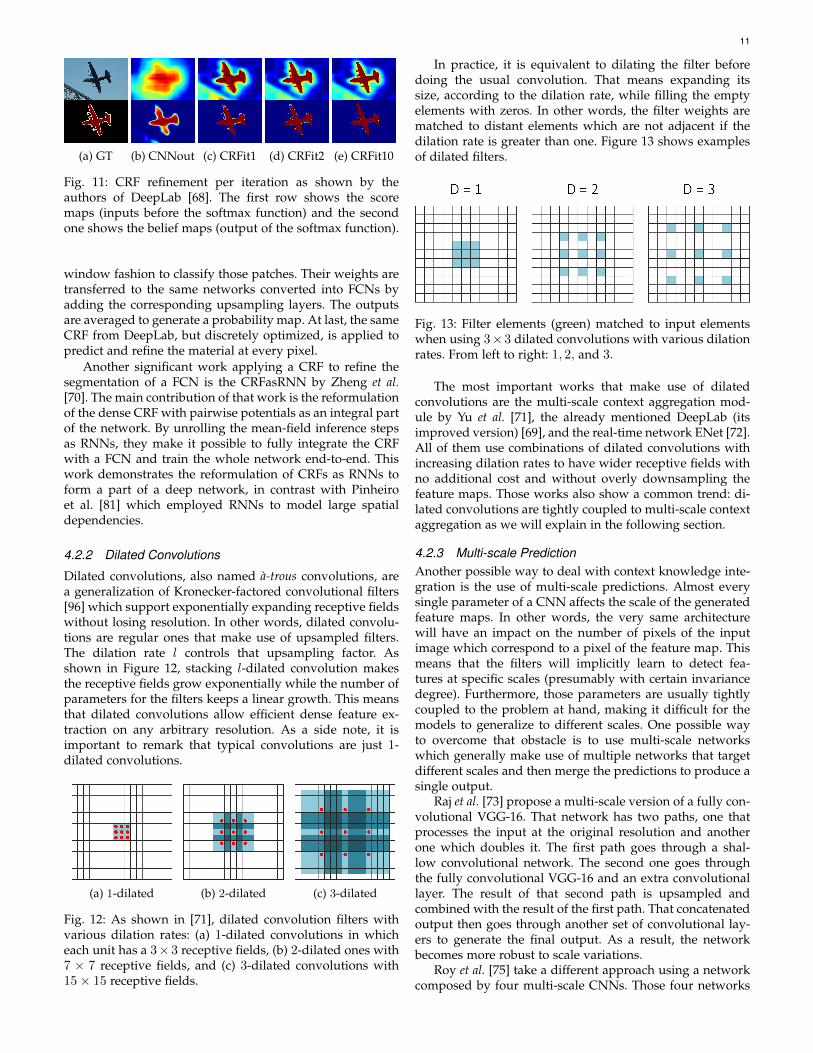
The DeepLab models [68] [69] make use of the fullyconnected pairwise CRF by Krahenbuhl and Koltun [94][95] as a separated post-processing step in their pipelineto refine the segmentation result. It models each pixel as anode in the field and employs one pairwise term for eachpair of pixels no matter how far they lie (this model isknown as dense or fully connected factor graph). By usingthis model, both short and long-range interactions are takeninto account, rendering the system able to recover detailedstructures in the segmentation that were lost due to thespatial invariance of the CNN. Despite the fact that usuallyfully connected models are inefficient, this model can beefficiently approximated via probabilistic inference. Figure11 shows the effect of this CRF-based post-processing onthe score and belief maps produced by the DeepLab model.

The material recognition in the wild network by Bell et al.[43] makes use of various CNNs trained to identify patchesin the MINC database. Those CNNs are used on a sliding

11

(a) GT (b) CNNout (c) CRFit1 (d) CRFit2 (e) CRFit10

Fig. 11: CRF refinement per iteration as shown by theauthors of DeepLab [68]. The first row shows the scoremaps (inputs before the softmax function) and the secondone shows the belief maps (output of the softmax function).

window fashion to classify those patches. Their weights aretransferred to the same networks converted into FCNs byadding the corresponding upsampling layers. The outputsare averaged to generate a probability map. At last, the sameCRF from DeepLab, but discretely optimized, is applied topredict and refine the material at every pixel.

Another significant work applying a CRF to refine thesegmentation of a FCN is the CRFasRNN by Zheng et al.[70]. The main contribution of that work is the reformulationof the dense CRF with pairwise potentials as an integral partof the network. By unrolling the mean-field inference stepsas RNNs, they make it possible to fully integrate the CRFwith a FCN and train the whole network end-to-end. Thiswork demonstrates the reformulation of CRFs as RNNs toform a part of a deep network, in contrast with Pinheiroet al. [81] which employed RNNs to model large spatialdependencies.

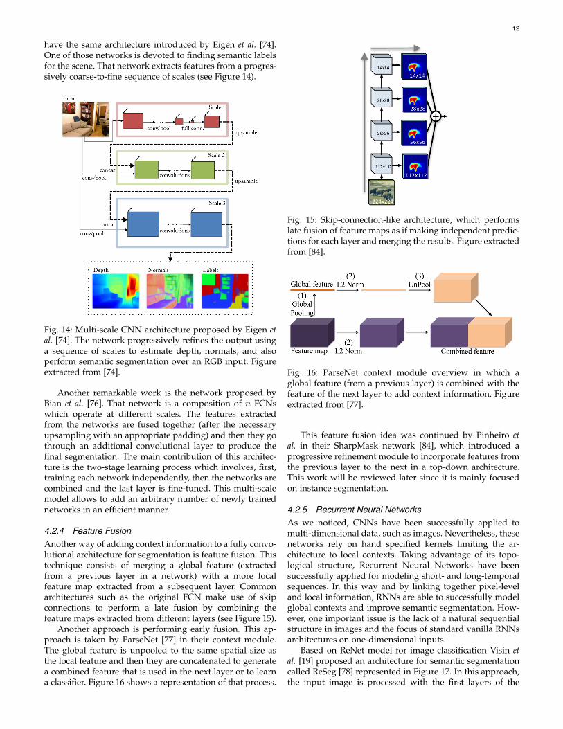
4.2.2 Dilated Convolutions

Dilated convolutions, also named a-trous convolutions, area generalization of Kronecker-factored convolutional filters[96] which support exponentially expanding receptive fieldswithout losing resolution. In other words, dilated convolu-tions are regular ones that make use of upsampled filters.The dilation rate l controls that upsampling factor. Asshown in Figure 12, stacking l-dilated convolution makesthe receptive fields grow exponentially while the number ofparameters for the filters keeps a linear growth. This meansthat dilated convolutions allow efficient dense feature ex-traction on any arbitrary resolution. As a side note, it isimportant to remark that typical convolutions are just 1-dilated convolutions.

(a) 1-dilated (b) 2-dilated (c) 3-dilated

Fig. 12: As shown in [71], dilated convolution filters withvarious dilation rates: (a) 1-dilated convolutions in whicheach unit has a 3× 3 receptive fields, (b) 2-dilated ones with7 × 7 receptive fields, and (c) 3-dilated convolutions with15× 15 receptive fields.

In practice, it is equivalent to dilating the filter beforedoing the usual convolution. That means expanding itssize, according to the dilation rate, while filling the emptyelements with zeros. In other words, the filter weights arematched to distant elements which are not adjacent if thedilation rate is greater than one. Figure 13 shows examplesof dilated filters.

Fig. 13: Filter elements (green) matched to input elementswhen using 3×3 dilated convolutions with various dilationrates. From left to right: 1, 2, and 3.

The most important works that make use of dilatedconvolutions are the multi-scale context aggregation mod-ule by Yu et al. [71], the already mentioned DeepLab (itsimproved version) [69], and the real-time network ENet [72].All of them use combinations of dilated convolutions withincreasing dilation rates to have wider receptive fields withno additional cost and without overly downsampling thefeature maps. Those works also show a common trend: di-lated convolutions are tightly coupled to multi-scale contextaggregation as we will explain in the following section.

4.2.3 Multi-scale PredictionAnother possible way to deal with context knowledge inte-gration is the use of multi-scale predictions. Almost everysingle parameter of a CNN affects the scale of the generatedfeature maps. In other words, the very same architecturewill have an impact on the number of pixels of the inputimage which correspond to a pixel of the feature map. Thismeans that the filters will implicitly learn to detect fea-tures at specific scales (presumably with certain invariancedegree). Furthermore, those parameters are usually tightlycoupled to the problem at hand, making it difficult for themodels to generalize to different scales. One possible wayto overcome that obstacle is to use multi-scale networkswhich generally make use of multiple networks that targetdifferent scales and then merge the predictions to produce asingle output.

Raj et al. [73] propose a multi-scale version of a fully con-volutional VGG-16. That network has two paths, one thatprocesses the input at the original resolution and anotherone which doubles it. The first path goes through a shal-low convolutional network. The second one goes throughthe fully convolutional VGG-16 and an extra convolutionallayer. The result of that second path is upsampled andcombined with the result of the first path. That concatenatedoutput then goes through another set of convolutional lay-ers to generate the final output. As a result, the networkbecomes more robust to scale variations.

Roy et al. [75] take a different approach using a networkcomposed by four multi-scale CNNs. Those four networks

12

have the same architecture introduced by Eigen et al. [74].One of those networks is devoted to finding semantic labelsfor the scene. That network extracts features from a progres-sively coarse-to-fine sequence of scales (see Figure 14).

Fig. 14: Multi-scale CNN architecture proposed by Eigen etal. [74]. The network progressively refines the output usinga sequence of scales to estimate depth, normals, and alsoperform semantic segmentation over an RGB input. Figureextracted from [74].

Another remarkable work is the network proposed byBian et al. [76]. That network is a composition of n FCNswhich operate at different scales. The features extractedfrom the networks are fused together (after the necessaryupsampling with an appropriate padding) and then they gothrough an additional convolutional layer to produce thefinal segmentation. The main contribution of this architec-ture is the two-stage learning process which involves, first,training each network independently, then the networks arecombined and the last layer is fine-tuned. This multi-scalemodel allows to add an arbitrary number of newly trainednetworks in an efficient manner.

4.2.4 Feature FusionAnother way of adding context information to a fully convo-lutional architecture for segmentation is feature fusion. Thistechnique consists of merging a global feature (extractedfrom a previous layer in a network) with a more localfeature map extracted from a subsequent layer. Commonarchitectures such as the original FCN make use of skipconnections to perform a late fusion by combining thefeature maps extracted from different layers (see Figure 15).

Another approach is performing early fusion. This ap-proach is taken by ParseNet [77] in their context module.The global feature is unpooled to the same spatial size asthe local feature and then they are concatenated to generatea combined feature that is used in the next layer or to learna classifier. Figure 16 shows a representation of that process.

Fig. 15: Skip-connection-like architecture, which performslate fusion of feature maps as if making independent predic-tions for each layer and merging the results. Figure extractedfrom [84].

Fig. 16: ParseNet context module overview in which aglobal feature (from a previous layer) is combined with thefeature of the next layer to add context information. Figureextracted from [77].

This feature fusion idea was continued by Pinheiro etal. in their SharpMask network [84], which introduced aprogressive refinement module to incorporate features fromthe previous layer to the next in a top-down architecture.This work will be reviewed later since it is mainly focusedon instance segmentation.

4.2.5 Recurrent Neural NetworksAs we noticed, CNNs have been successfully applied tomulti-dimensional data, such as images. Nevertheless, thesenetworks rely on hand specified kernels limiting the ar-chitecture to local contexts. Taking advantage of its topo-logical structure, Recurrent Neural Networks have beensuccessfully applied for modeling short- and long-temporalsequences. In this way and by linking together pixel-leveland local information, RNNs are able to successfully modelglobal contexts and improve semantic segmentation. How-ever, one important issue is the lack of a natural sequentialstructure in images and the focus of standard vanilla RNNsarchitectures on one-dimensional inputs.

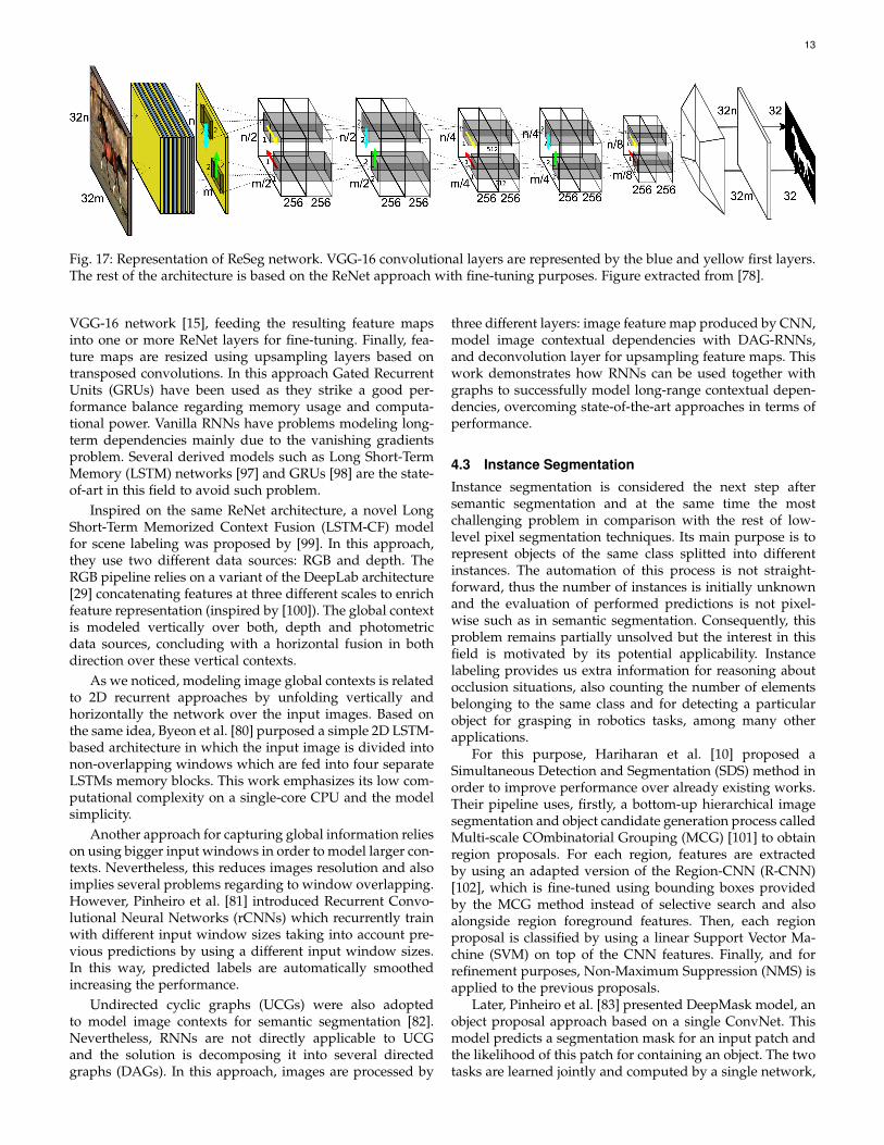
Based on ReNet model for image classification Visin etal. [19] proposed an architecture for semantic segmentationcalled ReSeg [78] represented in Figure 17. In this approach,the input image is processed with the first layers of the

13

Fig. 17: Representation of ReSeg network. VGG-16 convolutional layers are represented by the blue and yellow first layers.The rest of the architecture is based on the ReNet approach with fine-tuning purposes. Figure extracted from [78].

VGG-16 network [15], feeding the resulting feature mapsinto one or more ReNet layers for fine-tuning. Finally, fea-ture maps are resized using upsampling layers based ontransposed convolutions. In this approach Gated RecurrentUnits (GRUs) have been used as they strike a good per-formance balance regarding memory usage and computa-tional power. Vanilla RNNs have problems modeling long-term dependencies mainly due to the vanishing gradientsproblem. Several derived models such as Long Short-TermMemory (LSTM) networks [97] and GRUs [98] are the state-of-art in this field to avoid such problem.

Inspired on the same ReNet architecture, a novel LongShort-Term Memorized Context Fusion (LSTM-CF) modelfor scene labeling was proposed by [99]. In this approach,they use two different data sources: RGB and depth. TheRGB pipeline relies on a variant of the DeepLab architecture[29] concatenating features at three different scales to enrichfeature representation (inspired by [100]). The global contextis modeled vertically over both, depth and photometricdata sources, concluding with a horizontal fusion in bothdirection over these vertical contexts.

As we noticed, modeling image global contexts is relatedto 2D recurrent approaches by unfolding vertically andhorizontally the network over the input images. Based onthe same idea, Byeon et al. [80] purposed a simple 2D LSTM-based architecture in which the input image is divided intonon-overlapping windows which are fed into four separateLSTMs memory blocks. This work emphasizes its low com-putational complexity on a single-core CPU and the modelsimplicity.

Another approach for capturing global information relieson using bigger input windows in order to model larger con-texts. Nevertheless, this reduces images resolution and alsoimplies several problems regarding to window overlapping.However, Pinheiro et al. [81] introduced Recurrent Convo-lutional Neural Networks (rCNNs) which recurrently trainwith different input window sizes taking into account pre-vious predictions by using a different input window sizes.In this way, predicted labels are automatically smoothedincreasing the performance.

Undirected cyclic graphs (UCGs) were also adoptedto model image contexts for semantic segmentation [82].Nevertheless, RNNs are not directly applicable to UCGand the solution is decomposing it into several directedgraphs (DAGs). In this approach, images are processed by

three different layers: image feature map produced by CNN,model image contextual dependencies with DAG-RNNs,and deconvolution layer for upsampling feature maps. Thiswork demonstrates how RNNs can be used together withgraphs to successfully model long-range contextual depen-dencies, overcoming state-of-the-art approaches in terms ofperformance.

4.3 Instance Segmentation

Instance segmentation is considered the next step aftersemantic segmentation and at the same time the mostchallenging problem in comparison with the rest of low-level pixel segmentation techniques. Its main purpose is torepresent objects of the same class splitted into differentinstances. The automation of this process is not straight-forward, thus the number of instances is initially unknownand the evaluation of performed predictions is not pixel-wise such as in semantic segmentation. Consequently, thisproblem remains partially unsolved but the interest in thisfield is motivated by its potential applicability. Instancelabeling provides us extra information for reasoning aboutocclusion situations, also counting the number of elementsbelonging to the same class and for detecting a particularobject for grasping in robotics tasks, among many otherapplications.

For this purpose, Hariharan et al. [10] proposed aSimultaneous Detection and Segmentation (SDS) method inorder to improve performance over already existing works.Their pipeline uses, firstly, a bottom-up hierarchical imagesegmentation and object candidate generation process calledMulti-scale COmbinatorial Grouping (MCG) [101] to obtainregion proposals. For each region, features are extractedby using an adapted version of the Region-CNN (R-CNN)[102], which is fine-tuned using bounding boxes providedby the MCG method instead of selective search and alsoalongside region foreground features. Then, each regionproposal is classified by using a linear Support Vector Ma-chine (SVM) on top of the CNN features. Finally, and forrefinement purposes, Non-Maximum Suppression (NMS) isapplied to the previous proposals.

Later, Pinheiro et al. [83] presented DeepMask model, anobject proposal approach based on a single ConvNet. Thismodel predicts a segmentation mask for an input patch andthe likelihood of this patch for containing an object. The twotasks are learned jointly and computed by a single network,

14

sharing most of the layers except last ones which are task-specific.

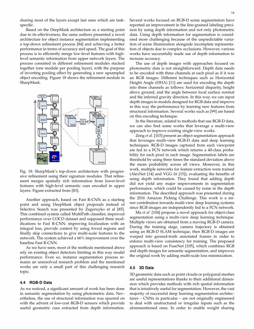
Based on the DeepMask architecture as a starting pointdue to its effectiveness, the same authors presented a novelarchitecture for object instance segmentation implementinga top-down refinement process [84] and achieving a betterperformance in terms of accuracy and speed. The goal of thisprocess is to efficiently merge low-level features with high-level semantic information from upper network layers. Theprocess consisted in different refinement modules stackedtogether (one module per pooling layer), with the purposeof inverting pooling effect by generating a new upsampledobject encoding. Figure 18 shows the refinement module inSharpMask.

Fig. 18: SharpMask’s top-down architecture with progres-sive refinement using their signature modules. That refine-ment merges spatially rich information from lower-levelfeatures with high-level semantic cues encoded in upperlayers. Figure extracted from [83].

Another approach, based on Fast R-CNN as a startingpoint and using DeepMask object proposals instead ofSelective Search was presented by Zagoruyko et al [85].This combined system called MultiPath classifier, improvedperformance over COCO dataset and supposed three mod-ifications to Fast R-CNN: improving localization with anintegral loss, provide context by using foveal regions andfinally skip connections to give multi-scale features to thenetwork. The system achieved a 66% improvement over thebaseline Fast R-CNN.

As we have seen, most of the methods mentioned aboverely on existing object detectors limiting in this way modelperformance. Even so, instance segmentation process re-mains an unresolved research problem and the mentionedworks are only a small part of this challenging researchtopic.

4.4 RGB-D DataAs we noticed, a significant amount of work has been donein semantic segmentation by using photometric data. Nev-ertheless, the use of structural information was spurred onwith the advent of low-cost RGB-D sensors which provideuseful geometric cues extracted from depth information.

Several works focused on RGB-D scene segmentation havereported an improvement in the fine-grained labeling preci-sion by using depth information and not only photometricdata. Using depth information for segmentation is consid-ered more challenging because of the unpredictable varia-tion of scene illumination alongside incomplete representa-tion of objects due to complex occlusions. However, variousworks have successfully made use of depth information toincrease accuracy.

The use of depth images with approaches focused onphotometric data is not straightforward. Depth data needsto be encoded with three channels at each pixel as if it wasan RGB images. Different techniques such as HorizontalHeight Angle (HHA) [11] are used for encoding the depthinto three channels as follows: horizontal disparity, heightabove ground, and the angle between local surface normaland the inferred gravity direction. In this way, we can inputdepth images to models designed for RGB data and improvein this way the performance by learning new features fromstructural information. Several works such as [99] are basedon this encoding technique.

In the literature, related to methods that use RGB-D data,we can also find some works that leverage a multi-viewapproach to improve existing single-view works.

Zeng et al. [103] present an object segmentation approachthat leverages multi-view RGB-D data and deep learningtechniques. RGB-D images captured from each viewpointare fed to a FCN network which returns a 40-class proba-bility for each pixel in each image. Segmentation labels arethreshold by using three times the standard deviation abovethe mean probability across all views. Moreover, in thiswork, multiple networks for feature extraction were trained(AlexNet [14] and VGG-16 [15]), evaluating the benefits ofusing depth information. They found that adding depthdid not yield any major improvements in segmentationperformance, which could be caused by noise in the depthinformation. The described approach was presented duringthe 2016 Amazon Picking Challenge. This work is a mi-nor contribution towards multi-view deep learning systemssince RGB images are independently fed to a FCN network.

Ma et al. [104] propose a novel approach for object-classsegmentation using a multi-view deep learning technique.Multiple views are obtained from a moving RGB-D camera.During the training stage, camera trajectory is obtainedusing an RGB-D SLAM technique, then RGB-D images arewarped into ground-truth annotated frames in order toenforce multi-view consistency for training. The proposedapproach is based on FuseNet [105], which combines RGBand depth images for semantic segmentation, and improvesthe original work by adding multi-scale loss minimization.

4.5 3D Data

3D geometric data such as point clouds or polygonal meshesare useful representations thanks to their additional dimen-sion which provides methods with rich spatial informationthat is intuitively useful for segmentation. However, the vastmajority of successful deep learning segmentation architec-tures – CNNs in particular – are not originally engineeredto deal with unstructured or irregular inputs such as theaforementioned ones. In order to enable weight sharing

15

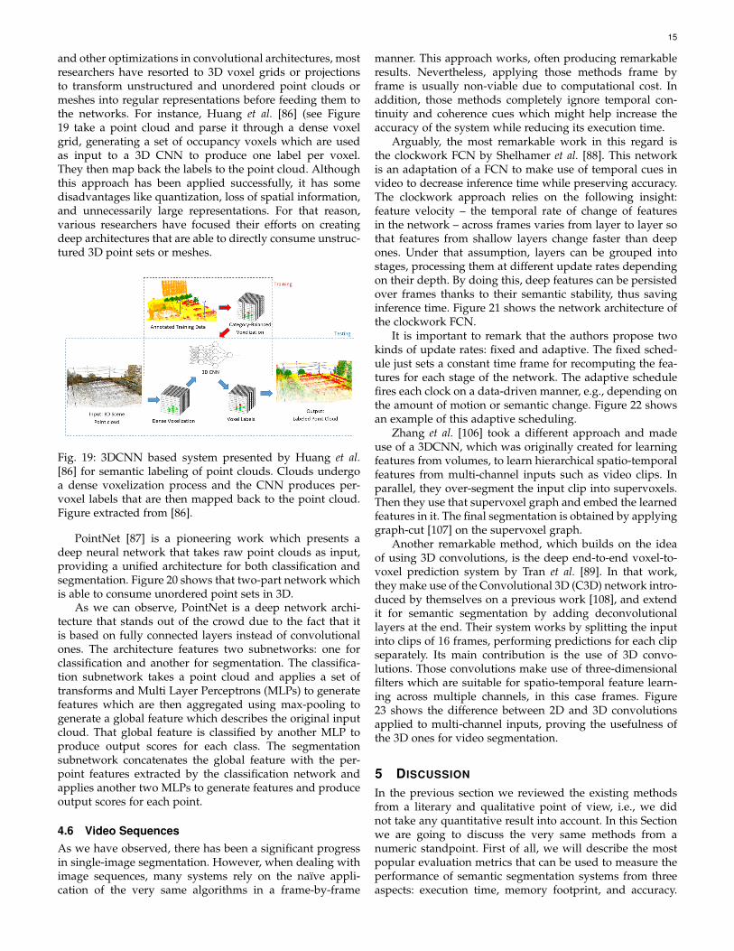
and other optimizations in convolutional architectures, mostresearchers have resorted to 3D voxel grids or projectionsto transform unstructured and unordered point clouds ormeshes into regular representations before feeding them tothe networks. For instance, Huang et al. [86] (see Figure19 take a point cloud and parse it through a dense voxelgrid, generating a set of occupancy voxels which are usedas input to a 3D CNN to produce one label per voxel.They then map back the labels to the point cloud. Althoughthis approach has been applied successfully, it has somedisadvantages like quantization, loss of spatial information,and unnecessarily large representations. For that reason,various researchers have focused their efforts on creatingdeep architectures that are able to directly consume unstruc-tured 3D point sets or meshes.

Fig. 19: 3DCNN based system presented by Huang et al.[86] for semantic labeling of point clouds. Clouds undergoa dense voxelization process and the CNN produces per-voxel labels that are then mapped back to the point cloud.Figure extracted from [86].

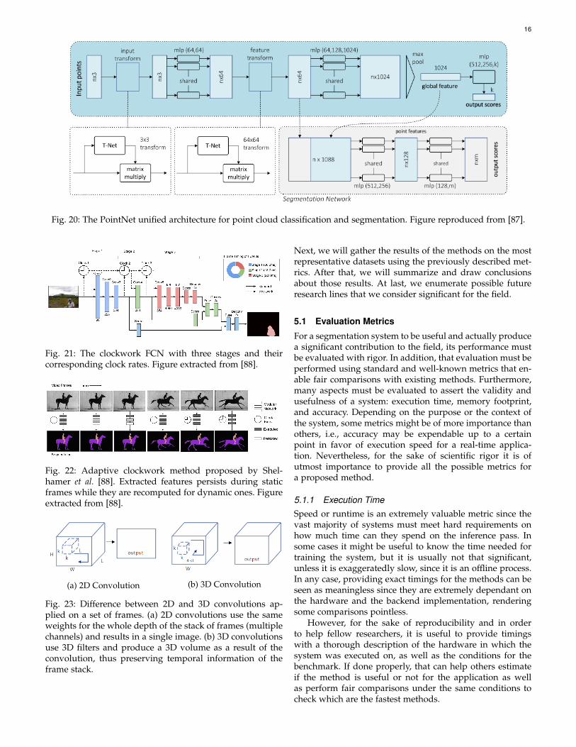
PointNet [87] is a pioneering work which presents adeep neural network that takes raw point clouds as input,providing a unified architecture for both classification andsegmentation. Figure 20 shows that two-part network whichis able to consume unordered point sets in 3D.

As we can observe, PointNet is a deep network archi-tecture that stands out of the crowd due to the fact that itis based on fully connected layers instead of convolutionalones. The architecture features two subnetworks: one forclassification and another for segmentation. The classifica-tion subnetwork takes a point cloud and applies a set oftransforms and Multi Layer Perceptrons (MLPs) to generatefeatures which are then aggregated using max-pooling togenerate a global feature which describes the original inputcloud. That global feature is classified by another MLP toproduce output scores for each class. The segmentationsubnetwork concatenates the global feature with the per-point features extracted by the classification network andapplies another two MLPs to generate features and produceoutput scores for each point.

4.6 Video SequencesAs we have observed, there has been a significant progressin single-image segmentation. However, when dealing withimage sequences, many systems rely on the naıve appli-cation of the very same algorithms in a frame-by-frame

manner. This approach works, often producing remarkableresults. Nevertheless, applying those methods frame byframe is usually non-viable due to computational cost. Inaddition, those methods completely ignore temporal con-tinuity and coherence cues which might help increase theaccuracy of the system while reducing its execution time.

Arguably, the most remarkable work in this regard isthe clockwork FCN by Shelhamer et al. [88]. This networkis an adaptation of a FCN to make use of temporal cues invideo to decrease inference time while preserving accuracy.The clockwork approach relies on the following insight:feature velocity – the temporal rate of change of featuresin the network – across frames varies from layer to layer sothat features from shallow layers change faster than deepones. Under that assumption, layers can be grouped intostages, processing them at different update rates dependingon their depth. By doing this, deep features can be persistedover frames thanks to their semantic stability, thus savinginference time. Figure 21 shows the network architecture ofthe clockwork FCN.

It is important to remark that the authors propose twokinds of update rates: fixed and adaptive. The fixed sched-ule just sets a constant time frame for recomputing the fea-tures for each stage of the network. The adaptive schedulefires each clock on a data-driven manner, e.g., depending onthe amount of motion or semantic change. Figure 22 showsan example of this adaptive scheduling.

Zhang et al. [106] took a different approach and madeuse of a 3DCNN, which was originally created for learningfeatures from volumes, to learn hierarchical spatio-temporalfeatures from multi-channel inputs such as video clips. Inparallel, they over-segment the input clip into supervoxels.Then they use that supervoxel graph and embed the learnedfeatures in it. The final segmentation is obtained by applyinggraph-cut [107] on the supervoxel graph.

Another remarkable method, which builds on the ideaof using 3D convolutions, is the deep end-to-end voxel-to-voxel prediction system by Tran et al. [89]. In that work,they make use of the Convolutional 3D (C3D) network intro-duced by themselves on a previous work [108], and extendit for semantic segmentation by adding deconvolutionallayers at the end. Their system works by splitting the inputinto clips of 16 frames, performing predictions for each clipseparately. Its main contribution is the use of 3D convo-lutions. Those convolutions make use of three-dimensionalfilters which are suitable for spatio-temporal feature learn-ing across multiple channels, in this case frames. Figure23 shows the difference between 2D and 3D convolutionsapplied to multi-channel inputs, proving the usefulness ofthe 3D ones for video segmentation.

5 DISCUSSION

In the previous section we reviewed the existing methodsfrom a literary and qualitative point of view, i.e., we didnot take any quantitative result into account. In this Sectionwe are going to discuss the very same methods from anumeric standpoint. First of all, we will describe the mostpopular evaluation metrics that can be used to measure theperformance of semantic segmentation systems from threeaspects: execution time, memory footprint, and accuracy.

16

Fig. 20: The PointNet unified architecture for point cloud classification and segmentation. Figure reproduced from [87].

Fig. 21: The clockwork FCN with three stages and theircorresponding clock rates. Figure extracted from [88].

Fig. 22: Adaptive clockwork method proposed by Shel-hamer et al. [88]. Extracted features persists during staticframes while they are recomputed for dynamic ones. Figureextracted from [88].

(a) 2D Convolution (b) 3D Convolution

Fig. 23: Difference between 2D and 3D convolutions ap-plied on a set of frames. (a) 2D convolutions use the sameweights for the whole depth of the stack of frames (multiplechannels) and results in a single image. (b) 3D convolutionsuse 3D filters and produce a 3D volume as a result of theconvolution, thus preserving temporal information of theframe stack.

Next, we will gather the results of the methods on the mostrepresentative datasets using the previously described met-rics. After that, we will summarize and draw conclusionsabout those results. At last, we enumerate possible futureresearch lines that we consider significant for the field.

5.1 Evaluation Metrics

For a segmentation system to be useful and actually producea significant contribution to the field, its performance mustbe evaluated with rigor. In addition, that evaluation must beperformed using standard and well-known metrics that en-able fair comparisons with existing methods. Furthermore,many aspects must be evaluated to assert the validity andusefulness of a system: execution time, memory footprint,and accuracy. Depending on the purpose or the context ofthe system, some metrics might be of more importance thanothers, i.e., accuracy may be expendable up to a certainpoint in favor of execution speed for a real-time applica-tion. Nevertheless, for the sake of scientific rigor it is ofutmost importance to provide all the possible metrics fora proposed method.

5.1.1 Execution TimeSpeed or runtime is an extremely valuable metric since thevast majority of systems must meet hard requirements onhow much time can they spend on the inference pass. Insome cases it might be useful to know the time needed fortraining the system, but it is usually not that significant,unless it is exaggeratedly slow, since it is an offline process.In any case, providing exact timings for the methods can beseen as meaningless since they are extremely dependant onthe hardware and the backend implementation, renderingsome comparisons pointless.

However, for the sake of reproducibility and in orderto help fellow researchers, it is useful to provide timingswith a thorough description of the hardware in which thesystem was executed on, as well as the conditions for thebenchmark. If done properly, that can help others estimateif the method is useful or not for the application as wellas perform fair comparisons under the same conditions tocheck which are the fastest methods.

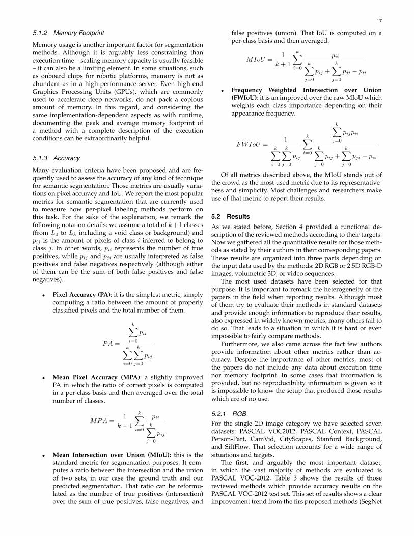
17

5.1.2 Memory Footprint

Memory usage is another important factor for segmentationmethods. Although it is arguably less constraining thanexecution time – scaling memory capacity is usually feasible– it can also be a limiting element. In some situations, suchas onboard chips for robotic platforms, memory is not asabundant as in a high-performance server. Even high-endGraphics Processing Units (GPUs), which are commonlyused to accelerate deep networks, do not pack a copiousamount of memory. In this regard, and considering thesame implementation-dependent aspects as with runtime,documenting the peak and average memory footprint ofa method with a complete description of the executionconditions can be extraordinarily helpful.

5.1.3 Accuracy

Many evaluation criteria have been proposed and are fre-quently used to assess the accuracy of any kind of techniquefor semantic segmentation. Those metrics are usually varia-tions on pixel accuracy and IoU. We report the most popularmetrics for semantic segmentation that are currently usedto measure how per-pixel labeling methods perform onthis task. For the sake of the explanation, we remark thefollowing notation details: we assume a total of k+1 classes(from L0 to Lk including a void class or background) andpij is the amount of pixels of class i inferred to belong toclass j. In other words, pii represents the number of truepositives, while pij and pji are usually interpreted as falsepositives and false negatives respectively (although eitherof them can be the sum of both false positives and falsenegatives)..

• Pixel Accuracy (PA): it is the simplest metric, simplycomputing a ratio between the amount of properlyclassified pixels and the total number of them.

PA =

k∑i=0

pii

k∑i=0

k∑j=0

pij

• Mean Pixel Accuracy (MPA): a slightly improvedPA in which the ratio of correct pixels is computedin a per-class basis and then averaged over the totalnumber of classes.

MPA =1

k + 1

k∑i=0

piik∑

j=0

pij

• Mean Intersection over Union (MIoU): this is thestandard metric for segmentation purposes. It com-putes a ratio between the intersection and the unionof two sets, in our case the ground truth and ourpredicted segmentation. That ratio can be reformu-lated as the number of true positives (intersection)over the sum of true positives, false negatives, and

false positives (union). That IoU is computed on aper-class basis and then averaged.

MIoU =1

k + 1

k∑i=0

piik∑

j=0

pij +

k∑j=0

pji − pii

• Frequency Weighted Intersection over Union(FWIoU): it is an improved over the raw MIoU whichweights each class importance depending on theirappearance frequency.

FWIoU =1

k∑i=0

k∑j=0

pij

k∑i=0

k∑j=0

pijpii

k∑j=0

pij +

k∑j=0

pji − pii

Of all metrics described above, the MIoU stands out ofthe crowd as the most used metric due to its representative-ness and simplicity. Most challenges and researchers makeuse of that metric to report their results.

5.2 ResultsAs we stated before, Section 4 provided a functional de-scription of the reviewed methods according to their targets.Now we gathered all the quantitative results for those meth-ods as stated by their authors in their corresponding papers.These results are organized into three parts depending onthe input data used by the methods: 2D RGB or 2.5D RGB-Dimages, volumetric 3D, or video sequences.

The most used datasets have been selected for thatpurpose. It is important to remark the heterogeneity of thepapers in the field when reporting results. Although mostof them try to evaluate their methods in standard datasetsand provide enough information to reproduce their results,also expressed in widely known metrics, many others fail todo so. That leads to a situation in which it is hard or evenimpossible to fairly compare methods.

Furthermore, we also came across the fact few authorsprovide information about other metrics rather than ac-curacy. Despite the importance of other metrics, most ofthe papers do not include any data about execution timenor memory footprint. In some cases that information isprovided, but no reproducibility information is given so itis impossible to know the setup that produced those resultswhich are of no use.

5.2.1 RGBFor the single 2D image category we have selected sevendatasets: PASCAL VOC2012, PASCAL Context, PASCALPerson-Part, CamVid, CityScapes, Stanford Background,and SiftFlow. That selection accounts for a wide range ofsituations and targets.

The first, and arguably the most important dataset,in which the vast majority of methods are evaluated isPASCAL VOC-2012. Table 3 shows the results of thosereviewed methods which provide accuracy results on thePASCAL VOC-2012 test set. This set of results shows a clearimprovement trend from the firs proposed methods (SegNet

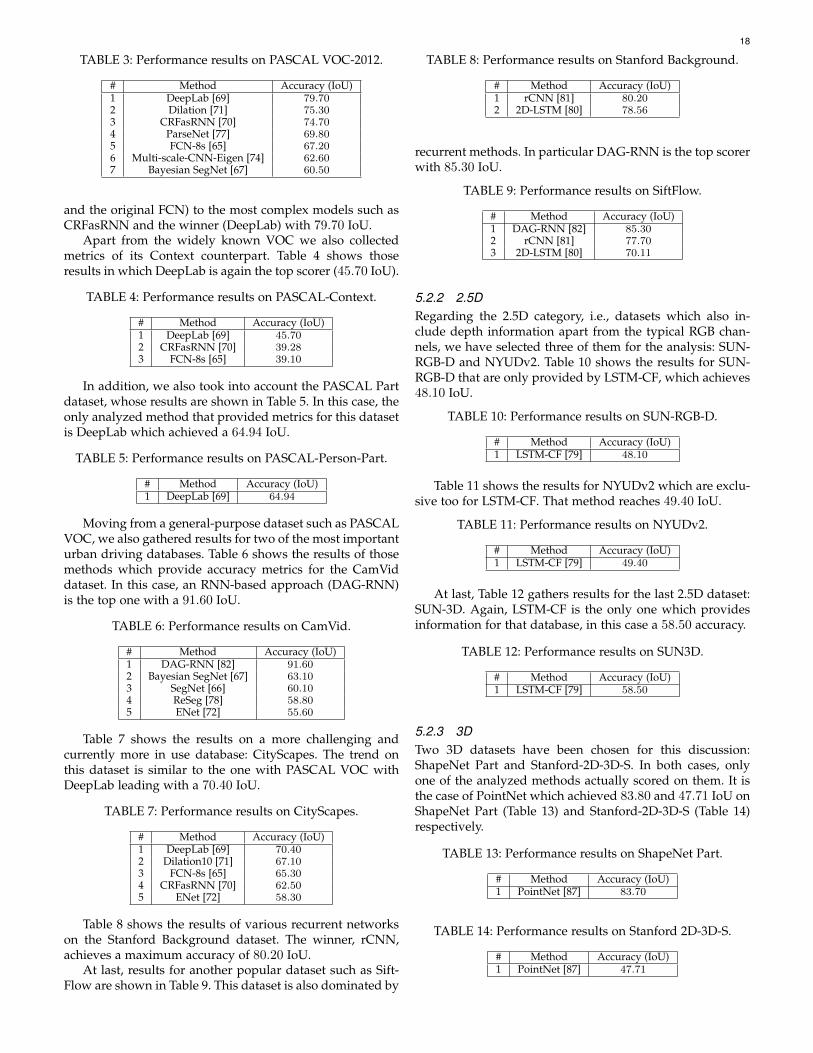
18

TABLE 3: Performance results on PASCAL VOC-2012.

# Method Accuracy (IoU)1 DeepLab [69] 79.702 Dilation [71] 75.303 CRFasRNN [70] 74.704 ParseNet [77] 69.805 FCN-8s [65] 67.206 Multi-scale-CNN-Eigen [74] 62.607 Bayesian SegNet [67] 60.50

and the original FCN) to the most complex models such asCRFasRNN and the winner (DeepLab) with 79.70 IoU.

Apart from the widely known VOC we also collectedmetrics of its Context counterpart. Table 4 shows thoseresults in which DeepLab is again the top scorer (45.70 IoU).

TABLE 4: Performance results on PASCAL-Context.

# Method Accuracy (IoU)1 DeepLab [69] 45.702 CRFasRNN [70] 39.283 FCN-8s [65] 39.10

In addition, we also took into account the PASCAL Partdataset, whose results are shown in Table 5. In this case, theonly analyzed method that provided metrics for this datasetis DeepLab which achieved a 64.94 IoU.

TABLE 5: Performance results on PASCAL-Person-Part.

# Method Accuracy (IoU)1 DeepLab [69] 64.94

Moving from a general-purpose dataset such as PASCALVOC, we also gathered results for two of the most importanturban driving databases. Table 6 shows the results of thosemethods which provide accuracy metrics for the CamViddataset. In this case, an RNN-based approach (DAG-RNN)is the top one with a 91.60 IoU.

TABLE 6: Performance results on CamVid.

# Method Accuracy (IoU)1 DAG-RNN [82] 91.602 Bayesian SegNet [67] 63.103 SegNet [66] 60.104 ReSeg [78] 58.805 ENet [72] 55.60

Table 7 shows the results on a more challenging andcurrently more in use database: CityScapes. The trend onthis dataset is similar to the one with PASCAL VOC withDeepLab leading with a 70.40 IoU.

TABLE 7: Performance results on CityScapes.

# Method Accuracy (IoU)1 DeepLab [69] 70.402 Dilation10 [71] 67.103 FCN-8s [65] 65.304 CRFasRNN [70] 62.505 ENet [72] 58.30

Table 8 shows the results of various recurrent networkson the Stanford Background dataset. The winner, rCNN,achieves a maximum accuracy of 80.20 IoU.

At last, results for another popular dataset such as Sift-Flow are shown in Table 9. This dataset is also dominated by

TABLE 8: Performance results on Stanford Background.

# Method Accuracy (IoU)1 rCNN [81] 80.202 2D-LSTM [80] 78.56

recurrent methods. In particular DAG-RNN is the top scorerwith 85.30 IoU.

TABLE 9: Performance results on SiftFlow.

# Method Accuracy (IoU)1 DAG-RNN [82] 85.302 rCNN [81] 77.703 2D-LSTM [80] 70.11

5.2.2 2.5DRegarding the 2.5D category, i.e., datasets which also in-clude depth information apart from the typical RGB chan-nels, we have selected three of them for the analysis: SUN-RGB-D and NYUDv2. Table 10 shows the results for SUN-RGB-D that are only provided by LSTM-CF, which achieves48.10 IoU.

TABLE 10: Performance results on SUN-RGB-D.

# Method Accuracy (IoU)1 LSTM-CF [79] 48.10

Table 11 shows the results for NYUDv2 which are exclu-sive too for LSTM-CF. That method reaches 49.40 IoU.

TABLE 11: Performance results on NYUDv2.

# Method Accuracy (IoU)1 LSTM-CF [79] 49.40

At last, Table 12 gathers results for the last 2.5D dataset:SUN-3D. Again, LSTM-CF is the only one which providesinformation for that database, in this case a 58.50 accuracy.

TABLE 12: Performance results on SUN3D.

# Method Accuracy (IoU)1 LSTM-CF [79] 58.50

5.2.3 3DTwo 3D datasets have been chosen for this discussion:ShapeNet Part and Stanford-2D-3D-S. In both cases, onlyone of the analyzed methods actually scored on them. It isthe case of PointNet which achieved 83.80 and 47.71 IoU onShapeNet Part (Table 13) and Stanford-2D-3D-S (Table 14)respectively.

TABLE 13: Performance results on ShapeNet Part.

# Method Accuracy (IoU)1 PointNet [87] 83.70

TABLE 14: Performance results on Stanford 2D-3D-S.

# Method Accuracy (IoU)1 PointNet [87] 47.71

19

5.2.4 Sequences

The last category included in this discussion is video orsequences. For that part we gathered results for two datasetswhich are suitable for sequence segmentation: CityScapesand YouTube-Objects. Only one of the reviewed methods forvideo segmentation provides quantitative results on thosedatasets: Clockwork Convnet. That method reaches 64.40IoU on CityScapes (Table 15), and 68.50 on YouTube-Objects(Table 16).

TABLE 15: Performance results on Cityscapes.

# Method Accuracy (IoU)1 Clockwork Convnet [88] 64.40

TABLE 16: Performance results on Youtube-Objects.

# Method Accuracy (IoU)1 Clockwork Convnet [88] 68.50

5.3 Summary

In light of the results, we can draw various conclusions.The most important of them is related to reproducibility. Aswe have observed, many methods report results on non-standard datasets or they are not even tested at all. Thatmakes comparisons impossible. Furthermore, some of themdo not describe the setup for the experimentation or donot provide the source code for the implementation, thussignificantly hurting reproducibility. Methods should reporttheir results on standard datasets, exhaustively describe thetraining procedure, and also make their models and weightspublicly available to enable progress.

Another important fact discovered thanks to this studyis the lack of information about other metrics such as exe-cution time and memory footprint. Almost no paper reportsthis kind of information, and those who do suffer from thereproducibility issues mentioned before. This void is dueto the fact that most methods focus on accuracy withoutany concern about time or space. However, it is importantto think about where are those methods being applied. Inpractice, most of them will end up running on embeddeddevices, e.g., self-driving cars, drones, or robots, which arefairly limited from both sides: computational power andmemory.

Regarding the results themselves, we can conclude thatDeepLab is the most solid method which outperformsthe rest on almost every single RGB images dataset by asignificant margin. The 2.5D or multimodal datasets aredominated by recurrent networks such as LSTM-CF. 3Ddata segmentation still has a long way to go with Point-Net paving the way for future research on dealing withunordered point clouds without any kind of preprocessingor discretization. Finally, dealing with video sequences isanother green area with no clear direction, but ClockworkConvnets are the most promising approach thanks to theirefficiency and accuracy duality. 3D convolutions are worthremarking due to their power and flexibility to processmultichannel inputs, making them successful at capturingboth spatial and temporal information.

5.4 Future Research Directions

Based on the reviewed research, which marks the state of theart of the field, we present a list of future research directionsthat would be interesting to pursue.

• 3D datasets: methods that make full use of 3D infor-mation are starting to rise but, even if new proposalsand techniques are engineered, they still lack oneof the most important components: data. There is astrong need for large-scale datasets for 3D semanticsegmentation, which are harder to create than theirlower dimensional counterparts. Although there arealready some promising works, there is still roomfor more, better, and varied data. It is important toremark the importance of real-world 3D data sincemost of the already existing works are syntheticdatabases. A proof of the importance of 3D is thefact that the ILSVRC will feature 3D data in 2018.

• Sequence datasets: the same lack of large-scale datathat hinders progress on 3D segmentation also im-pacts video segmentation. There are only a fewdatasets that are sequence-based and thus helpful fordeveloping methods which take advantage of tempo-ral information. Bringing up more high-quality datafrom this nature, either 2D or 3D, will unlock newresearch lines without any doubt.

• Point cloud segmentation using Graph ConvolutionalNetworks (GCNs): as we already mentioned, dealingwith 3D data such as point clouds poses an unsolvedchallenge. Due to its unordered and unstructurednature, traditional architectures such as CNNs can-not be applied unless some sort of discretizationprocess is applied to structure it. One promising lineof research aims to treat point clouds as graphs andapply convolutions over them [109] [110] [111]. Thishas the advantage of preserving spatial cues in everydimension without quantizing data.

• Context knowledge: while FCNs are a consolidatedapproach for semantic segmentation, they lack sev-eral features such as context modelling that helpincreasing accuracy. The reformulation of CRFs asRNNs to create end-to-end solutions seems to be apromising direction to improve results on real-lifedata. Multi-scale and feature fusion approaches havealso shown remarkable progress. In general, all thoseworks represent important steps towards achievingthe ultimate goal, but there are some problems thatstill require more research.

• Real-time segmentation: In many applications, preci-sion is important; however, it is also crucial that theseimplementations are able to cope with common cam-era frame rates (at least 25 frames per second). Mostof the current methods are far from that framerate,e.g., FCN-8s takes roughly 100 ms to process a low-resolution PASCAL VOC image whilst CRFasRNNneeds more than 500 ms. Therefore, during the nextyears, we expect a stream of works coming out,focusing more on real-time constraints. These futureworks will have to find a trade-off between accuracyand runtime.

20

• Memory: some platforms are bounded by hard mem-ory constraints. Segmentation networks usually doneed significant amounts of memory to be executedfor both inference and training. In order to fit themin some devices, networks must be simplified. Whilethis can be easily accomplished by reducing theircomplexity (often trading it for accuracy), anotherapproaches can be taken. Pruning is a promising re-search line that aims to simplify a network, making itlightweight while keeping the knowledge, and thusthe accuracy, of the original network architecture[112] [113] [114].

• Temporal coherency on sequences: some methods haveaddressed video or sequence segmentation but eithertaking advantage of that temporal cues to increaseaccuracy or efficiency. However, none of them haveexplicitly tackled the coherency problem. For a seg-mentation system to work on video streams it isimportant, not only to produce good results frameby frame, but also make them coherent through thewhole clip without producing artifacts by smoothingpredicted per-pixel labels along the sequence.

• Multi-view integration: Use of multiple views in re-cently proposed segmentation works is mostly lim-ited to RGB-D cameras and in particular focused onsingle-object segmentation.

6 CONCLUSION

To the best of our knowledge, this is the first review paperin the literature which focuses on semantic segmentationusing deep learning. In comparison with other surveys, thispaper is devoted to such a rising topic as deep learning,covering the most advanced and recent work on that front.We formulated the semantic segmentation problem andprovided the reader with the necessary background knowl-edge about deep learning for such task. We covered thecontemporary literature of datasets and methods, providinga comprehensive survey of 28 datasets and 27 methods.Datasets were carefully described, stating their purposesand characteristics so that researchers can easily pick the onethat best suits their needs. Methods were surveyed from twoperspectives: contributions and raw results, i.e., accuracy.We also presented a comparative summary of the datasetsand methods in tabular forms, classifying them accordingto various criteria. In the end, we discussed the resultsand provided useful insight in shape of future researchdirections and open problems in the field. In conclusion,semantic segmentation has been approached with manysuccess stories but still remains an open problem whosesolution would prove really useful for a wide set of real-world applications. Furthermore, deep learning has provedto be extremely powerful to tackle this problem so we canexpect a flurry of innovation and spawns of research linesin the upcoming years.

ACKNOWLEDGMENTS

This work has been funded by the Spanish GovernmentTIN2016-76515-R grant for the COMBAHO project, sup-ported with Feder funds. It has also been supported by

a Spanish national grant for PhD studies FPU15/04516.In addition, it was also funded by the grant Ayudas paraEstudios de Master e Iniciacion a la Investigacion from theUniversity of Alicante.

REFERENCES

[1] A. Ess, T. Muller, H. Grabner, and L. J. Van Gool, “Segmentation-based urban traffic scene understanding.” in BMVC, vol. 1, 2009,p. 2.

[2] A. Geiger, P. Lenz, and R. Urtasun, “Are we ready for au-tonomous driving? the kitti vision benchmark suite,” in 2012IEEE Conference on Computer Vision and Pattern Recognition, June2012, pp. 3354–3361.

[3] M. Cordts, M. Omran, S. Ramos, T. Rehfeld, M. Enzweiler,R. Benenson, U. Franke, S. Roth, and B. Schiele, “The cityscapesdataset for semantic urban scene understanding,” in Proceedingsof the IEEE Conference on Computer Vision and Pattern Recognition,2016, pp. 3213–3223.

[4] M. Oberweger, P. Wohlhart, and V. Lepetit, “Hands deepin deep learning for hand pose estimation,” arXiv preprintarXiv:1502.06807, 2015.

[5] Y. Yoon, H.-G. Jeon, D. Yoo, J.-Y. Lee, and I. So Kweon, “Learn-ing a deep convolutional network for light-field image super-resolution,” in Proceedings of the IEEE International Conference onComputer Vision Workshops, 2015, pp. 24–32.

[6] J. Wan, D. Wang, S. C. H. Hoi, P. Wu, J. Zhu, Y. Zhang, and J. Li,“Deep learning for content-based image retrieval: A comprehen-sive study,” in Proceedings of the 22nd ACM international conferenceon Multimedia. ACM, 2014, pp. 157–166.

[7] F. Ning, D. Delhomme, Y. LeCun, F. Piano, L. Bottou, and P. E.Barbano, “Toward automatic phenotyping of developing em-bryos from videos,” IEEE Transactions on Image Processing, vol. 14,no. 9, pp. 1360–1371, 2005.

[8] D. Ciresan, A. Giusti, L. M. Gambardella, and J. Schmidhuber,“Deep neural networks segment neuronal membranes in electronmicroscopy images,” in Advances in neural information processingsystems, 2012, pp. 2843–2851.

[9] C. Farabet, C. Couprie, L. Najman, and Y. LeCun, “Learninghierarchical features for scene labeling,” IEEE transactions onpattern analysis and machine intelligence, vol. 35, no. 8, pp. 1915–1929, 2013.

[10] B. Hariharan, P. Arbelaez, R. Girshick, and J. Malik, “Simulta-neous detection and segmentation,” in European Conference onComputer Vision. Springer, 2014, pp. 297–312.

[11] S. Gupta, R. Girshick, P. Arbelaez, and J. Malik, “Learning richfeatures from rgb-d images for object detection and segmenta-tion,” in European Conference on Computer Vision. Springer, 2014,pp. 345–360.

[12] H. Zhu, F. Meng, J. Cai, and S. Lu, “Beyond pixels:A comprehensive survey from bottom-up to semanticimage segmentation and cosegmentation,” Journal of VisualCommunication and Image Representation, vol. 34, pp. 12 –27, 2016. [Online]. Available: http://www.sciencedirect.com/science/article/pii/S1047320315002035

[13] M. Thoma, “A survey of semantic segmentation,” CoRR, vol.abs/1602.06541, 2016. [Online]. Available: http://arxiv.org/abs/1602.06541

[14] A. Krizhevsky, I. Sutskever, and G. E. Hinton, “Imagenet classifi-cation with deep convolutional neural networks,” in Advances inneural information processing systems, 2012, pp. 1097–1105.

[15] K. Simonyan and A. Zisserman, “Very deep convolutionalnetworks for large-scale image recognition,” arXiv preprintarXiv:1409.1556, 2014.

[16] C. Szegedy, W. Liu, Y. Jia, P. Sermanet, S. Reed, D. Anguelov,D. Erhan, V. Vanhoucke, and A. Rabinovich, “Going deeper withconvolutions,” in Proceedings of the IEEE Conference on ComputerVision and Pattern Recognition, 2015, pp. 1–9.

[17] K. He, X. Zhang, S. Ren, and J. Sun, “Deep residual learningfor image recognition,” in Proceedings of the IEEE Conference onComputer Vision and Pattern Recognition, 2016, pp. 770–778.

[18] A. Graves, S. Fernandez, and J. Schmidhuber, “Multi-dimensional recurrent neural networks,” CoRR, vol.abs/0705.2011, 2007. [Online]. Available: http://arxiv.org/abs/0705.2011

21

[19] F. Visin, K. Kastner, K. Cho, M. Matteucci, A. C. Courville, andY. Bengio, “Renet: A recurrent neural network based alternativeto convolutional networks,” CoRR, vol. abs/1505.00393, 2015.[Online]. Available: http://arxiv.org/abs/1505.00393

[20] A. Ahmed, K. Yu, W. Xu, Y. Gong, and E. Xing, “Training hi-erarchical feed-forward visual recognition models using transferlearning from pseudo-tasks,” in European Conference on ComputerVision. Springer, 2008, pp. 69–82.

[21] M. Oquab, L. Bottou, I. Laptev, and J. Sivic, “Learning andtransferring mid-level image representations using convolutionalneural networks,” in Proceedings of the IEEE conference on computervision and pattern recognition, 2014, pp. 1717–1724.

[22] J. Yosinski, J. Clune, Y. Bengio, and H. Lipson, “How transferableare features in deep neural networks?” in Advances in neuralinformation processing systems, 2014, pp. 3320–3328.

[23] J. Deng, W. Dong, R. Socher, L.-J. Li, K. Li, and L. Fei-Fei, “Im-agenet: A large-scale hierarchical image database,” in ComputerVision and Pattern Recognition, 2009. CVPR 2009. IEEE Conferenceon. IEEE, 2009, pp. 248–255.

[24] O. Russakovsky, J. Deng, H. Su, J. Krause, S. Satheesh, S. Ma,Z. Huang, A. Karpathy, A. Khosla, M. Bernstein et al., “Imagenetlarge scale visual recognition challenge,” International Journal ofComputer Vision, vol. 115, no. 3, pp. 211–252, 2015.

[25] S. C. Wong, A. Gatt, V. Stamatescu, and M. D. McDonnell,“Understanding data augmentation for classification: when towarp?” CoRR, vol. abs/1609.08764, 2016. [Online]. Available:http://arxiv.org/abs/1609.08764

[26] X. Shen, A. Hertzmann, J. Jia, S. Paris, B. Price, E. Shechtman, andI. Sachs, “Automatic portrait segmentation for image stylization,”in Computer Graphics Forum, vol. 35, no. 2. Wiley Online Library,2016, pp. 93–102.

[27] M. Everingham, S. M. A. Eslami, L. Van Gool, C. K. I. Williams,J. Winn, and A. Zisserman, “The pascal visual object classes chal-lenge: A retrospective,” International Journal of Computer Vision,vol. 111, no. 1, pp. 98–136, Jan. 2015.

[28] R. Mottaghi, X. Chen, X. Liu, N.-G. Cho, S.-W. Lee, S. Fidler,R. Urtasun, and A. Yuille, “The role of context for object detectionand semantic segmentation in the wild,” in IEEE Conference onComputer Vision and Pattern Recognition (CVPR), 2014.

[29] X. Chen, R. Mottaghi, X. Liu, S. Fidler, R. Urtasun, and A. Yuille,“Detect what you can: Detecting and representing objects usingholistic models and body parts,” in IEEE Conference on ComputerVision and Pattern Recognition (CVPR), 2014.

[30] B. Hariharan, P. Arbelaez, L. Bourdev, S. Maji, and J. Malik,“Semantic contours from inverse detectors,” in 2011 InternationalConference on Computer Vision. IEEE, 2011, pp. 991–998.

[31] T.-Y. Lin, M. Maire, S. Belongie, J. Hays, P. Perona, D. Ramanan,P. Dollar, and C. L. Zitnick, “Microsoft coco: Common objects incontext,” in European Conference on Computer Vision. Springer,2014, pp. 740–755.

[32] G. Ros, L. Sellart, J. Materzynska, D. Vazquez, and A. M. Lopez,“The synthia dataset: A large collection of synthetic images forsemantic segmentation of urban scenes,” in Proceedings of the IEEEConference on Computer Vision and Pattern Recognition, 2016, pp.3234–3243.

[33] M. Cordts, M. Omran, S. Ramos, T. Scharwachter, M. Enzweiler,R. Benenson, U. Franke, S. Roth, and B. Schiele, “The cityscapesdataset,” in CVPR Workshop on The Future of Datasets in Vision,2015.

[34] G. J. Brostow, J. Fauqueur, and R. Cipolla, “Semantic objectclasses in video: A high-definition ground truth database,” Pat-tern Recognition Letters, vol. 30, no. 2, pp. 88–97, 2009.

[35] P. Sturgess, K. Alahari, L. Ladicky, and P. H. Torr, “Combiningappearance and structure from motion features for road sceneunderstanding,” in BMVC 2012-23rd British Machine Vision Con-ference. BMVA, 2009.

[36] J. M. Alvarez, T. Gevers, Y. LeCun, and A. M. Lopez, “Roadscene segmentation from a single image,” in European Conferenceon Computer Vision. Springer, 2012, pp. 376–389.

[37] G. Ros and J. M. Alvarez, “Unsupervised image transformationfor outdoor semantic labelling,” in Intelligent Vehicles Symposium(IV), 2015 IEEE. IEEE, 2015, pp. 537–542.

[38] G. Ros, S. Ramos, M. Granados, A. Bakhtiary, D. Vazquez, andA. M. Lopez, “Vision-based offline-online perception paradigmfor autonomous driving,” in Applications of Computer Vision(WACV), 2015 IEEE Winter Conference on. IEEE, 2015, pp. 231–238.

[39] R. Zhang, S. A. Candra, K. Vetter, and A. Zakhor, “Sensor fusionfor semantic segmentation of urban scenes,” in Robotics andAutomation (ICRA), 2015 IEEE International Conference on. IEEE,2015, pp. 1850–1857.

[40] S. Gould, R. Fulton, and D. Koller, “Decomposing a scene intogeometric and semantically consistent regions,” in Computer Vi-sion, 2009 IEEE 12th International Conference on. IEEE, 2009, pp.1–8.

[41] C. Liu, J. Yuen, and A. Torralba, “Nonparametric scene parsing:Label transfer via dense scene alignment,” in Computer Vision andPattern Recognition, 2009. CVPR 2009. IEEE Conference on. IEEE,2009, pp. 1972–1979.

[42] S. D. Jain and K. Grauman, “Supervoxel-consistent foregroundpropagation in video,” in European Conference on Computer Vision.Springer, 2014, pp. 656–671.

[43] S. Bell, P. Upchurch, N. Snavely, and K. Bala, “Material recog-nition in the wild with the materials in context database,” inProceedings of the IEEE conference on computer vision and patternrecognition, 2015, pp. 3479–3487.

[44] F. Perazzi, J. Pont-Tuset, B. McWilliams, L. Van Gool, M. Gross,and A. Sorkine-Hornung, “A benchmark dataset and evaluationmethodology for video object segmentation,” in Computer Visionand Pattern Recognition, 2016.

[45] J. Pont-Tuset, F. Perazzi, S. Caelles, P. Arbelaez, A. Sorkine-Hornung, and L. Van Gool, “The 2017 davis challenge on videoobject segmentation,” arXiv:1704.00675, 2017.

[46] N. Silberman, D. Hoiem, P. Kohli, and R. Fergus, “Indoor seg-mentation and support inference from rgbd images,” in EuropeanConference on Computer Vision. Springer, 2012, pp. 746–760.

[47] J. Xiao, A. Owens, and A. Torralba, “Sun3d: A database of bigspaces reconstructed using sfm and object labels,” in 2013 IEEEInternational Conference on Computer Vision, Dec 2013, pp. 1625–1632.

[48] S. Song, S. P. Lichtenberg, and J. Xiao, “Sun rgb-d: A rgb-dscene understanding benchmark suite,” in Proceedings of the IEEEconference on computer vision and pattern recognition, 2015, pp. 567–576.

[49] K. Lai, L. Bo, X. Ren, and D. Fox, “A large-scale hierarchicalmulti-view rgb-d object dataset,” in Robotics and Automation(ICRA), 2011 IEEE International Conference on. IEEE, 2011, pp.1817–1824.

[50] L. Yi, V. G. Kim, D. Ceylan, I.-C. Shen, M. Yan, H. Su, C. Lu,Q. Huang, A. Sheffer, and L. Guibas, “A scalable active frame-work for region annotation in 3d shape collections,” SIGGRAPHAsia, 2016.

[51] I. Armeni, A. Sax, A. R. Zamir, and S. Savarese, “Joint 2D-3D-Semantic Data for Indoor Scene Understanding,” ArXiv e-prints,Feb. 2017.

[52] X. Chen, A. Golovinskiy, and T. Funkhouser, “A benchmarkfor 3D mesh segmentation,” ACM Transactions on Graphics (Proc.SIGGRAPH), vol. 28, no. 3, Aug. 2009.

[53] A. Quadros, J. Underwood, and B. Douillard, “An occlusion-aware feature for range images,” in Robotics and Automation, 2012.ICRA’12. IEEE International Conference on. IEEE, May 14-18 2012.

[54] T. Hackel, J. D. Wegner, and K. Schindler, “Contour detectionin unstructured 3d point clouds,” in Proceedings of the IEEEConference on Computer Vision and Pattern Recognition, 2016, pp.1610–1618.

[55] G. J. Brostow, J. Shotton, J. Fauqueur, and R. Cipolla, “Segmenta-tion and recognition using structure from motion point clouds,”in European Conference on Computer Vision. Springer, 2008, pp.44–57.

[56] A. Geiger, P. Lenz, C. Stiller, and R. Urtasun, “Vision meetsrobotics: The kitti dataset,” The International Journal of RoboticsResearch, vol. 32, no. 11, pp. 1231–1237, 2013.

[57] A. Prest, C. Leistner, J. Civera, C. Schmid, and V. Ferrari, “Learn-ing object class detectors from weakly annotated video,” in Com-puter Vision and Pattern Recognition (CVPR), 2012 IEEE Conferenceon. IEEE, 2012, pp. 3282–3289.

[58] S. Bell, P. Upchurch, N. Snavely, and K. Bala, “OpenSurfaces: Arichly annotated catalog of surface appearance,” ACM Trans. onGraphics (SIGGRAPH), vol. 32, no. 4, 2013.

[59] B. C. Russell, A. Torralba, K. P. Murphy, and W. T. Freeman,“Labelme: a database and web-based tool for image annotation,”International journal of computer vision, vol. 77, no. 1, pp. 157–173,2008.

22

[60] S. Gupta, P. Arbelaez, and J. Malik, “Perceptual organization andrecognition of indoor scenes from rgb-d images,” in Proceedingsof the IEEE Conference on Computer Vision and Pattern Recognition,2013, pp. 564–571.

[61] A. Janoch, S. Karayev, Y. Jia, J. T. Barron, M. Fritz, K. Saenko, andT. Darrell, A Category-Level 3D Object Dataset: Putting the Kinectto Work. London: Springer London, 2013, pp. 141–165. [Online].Available: http://dx.doi.org/10.1007/978-1-4471-4640-7 8

[62] A. Richtsfeld, “The object segmentation database (osd),” 2012.[63] A. X. Chang, T. Funkhouser, L. Guibas, P. Hanrahan, Q. Huang,

Z. Li, S. Savarese, M. Savva, S. Song, H. Su et al., “Shapenet:An information-rich 3d model repository,” arXiv preprintarXiv:1512.03012, 2015.

[64] I. Armeni, O. Sener, A. R. Zamir, H. Jiang, I. Brilakis, M. Fischer,and S. Savarese, “3d semantic parsing of large-scale indoorspaces,” in Proceedings of the IEEE Conference on Computer Visionand Pattern Recognition, 2016, pp. 1534–1543.

[65] J. Long, E. Shelhamer, and T. Darrell, “Fully convolutional net-works for semantic segmentation,” in Proceedings of the IEEEConference on Computer Vision and Pattern Recognition, 2015, pp.3431–3440.

[66] V. Badrinarayanan, A. Kendall, and R. Cipolla, “Segnet: A deepconvolutional encoder-decoder architecture for image segmenta-tion,” arXiv preprint arXiv:1511.00561, 2015.

[67] A. Kendall, V. Badrinarayanan, and R. Cipolla, “Bayesiansegnet: Model uncertainty in deep convolutional encoder-decoder architectures for scene understanding,” arXiv preprintarXiv:1511.02680, 2015.

[68] L.-C. Chen, G. Papandreou, I. Kokkinos, K. Murphy, and A. L.Yuille, “Semantic image segmentation with deep convolutionalnets and fully connected crfs,” arXiv preprint arXiv:1412.7062,2014.

[69] ——, “Deeplab: Semantic image segmentation with deep convo-lutional nets, atrous convolution, and fully connected crfs,” arXivpreprint arXiv:1606.00915, 2016.

[70] S. Zheng, S. Jayasumana, B. Romera-Paredes, V. Vineet, Z. Su,D. Du, C. Huang, and P. H. Torr, “Conditional random fields asrecurrent neural networks,” in Proceedings of the IEEE InternationalConference on Computer Vision, 2015, pp. 1529–1537.

[71] F. Yu and V. Koltun, “Multi-scale context aggregation by dilatedconvolutions,” arXiv preprint arXiv:1511.07122, 2015.

[72] A. Paszke, A. Chaurasia, S. Kim, and E. Culurciello, “Enet: Adeep neural network architecture for real-time semantic segmen-tation,” arXiv preprint arXiv:1606.02147, 2016.

[73] A. Raj, D. Maturana, and S. Scherer, “Multi-scale convolutionalarchitecture for semantic segmentation,” 2015.

[74] D. Eigen and R. Fergus, “Predicting depth, surface normalsand semantic labels with a common multi-scale convolutionalarchitecture,” in Proceedings of the IEEE International Conference onComputer Vision, 2015, pp. 2650–2658.

[75] A. Roy and S. Todorovic, “A multi-scale cnn for affordancesegmentation in rgb images,” in European Conference on ComputerVision. Springer, 2016, pp. 186–201.

[76] X. Bian, S. N. Lim, and N. Zhou, “Multiscale fully convolutionalnetwork with application to industrial inspection,” in Applicationsof Computer Vision (WACV), 2016 IEEE Winter Conference on. IEEE,2016, pp. 1–8.

[77] W. Liu, A. Rabinovich, and A. C. Berg, “Parsenet: Looking widerto see better,” arXiv preprint arXiv:1506.04579, 2015.

[78] F. Visin, M. Ciccone, A. Romero, K. Kastner, K. Cho, Y. Bengio,M. Matteucci, and A. Courville, “Reseg: A recurrent neuralnetwork-based model for semantic segmentation,” in The IEEEConference on Computer Vision and Pattern Recognition (CVPR)Workshops, June 2016.

[79] Z. Li, Y. Gan, X. Liang, Y. Yu, H. Cheng, and L. Lin,LSTM-CF: Unifying Context Modeling and Fusion with LSTMsfor RGB-D Scene Labeling. Cham: Springer InternationalPublishing, 2016, pp. 541–557. [Online]. Available: http://dx.doi.org/10.1007/978-3-319-46475-6 34

[80] W. Byeon, T. M. Breuel, F. Raue, and M. Liwicki, “Scene labelingwith lstm recurrent neural networks,” in Proceedings of the IEEEConference on Computer Vision and Pattern Recognition, 2015, pp.3547–3555.

[81] P. H. Pinheiro and R. Collobert, “Recurrent convolutional neuralnetworks for scene labeling.” in ICML, 2014, pp. 82–90.

[82] B. Shuai, Z. Zuo, G. Wang, and B. Wang, “Dag-recurrent neuralnetworks for scene labeling,” CoRR, vol. abs/1509.00552, 2015.[Online]. Available: http://arxiv.org/abs/1509.00552

[83] P. O. Pinheiro, R. Collobert, and P. Dollar, “Learning to segmentobject candidates,” in Advances in Neural Information ProcessingSystems, 2015, pp. 1990–1998.

[84] P. O. Pinheiro, T.-Y. Lin, R. Collobert, and P. Dollar, “Learningto refine object segments,” in European Conference on ComputerVision. Springer, 2016, pp. 75–91.

[85] S. Zagoruyko, A. Lerer, T.-Y. Lin, P. O. Pinheiro, S. Gross, S. Chin-tala, and P. Dollar, “A multipath network for object detection,”arXiv preprint arXiv:1604.02135, 2016.

[86] J. Huang and S. You, “Point cloud labeling using 3d convolu-tional neural network,” in Proc. of the International Conf. on PatternRecognition (ICPR), vol. 2, 2016.

[87] C. R. Qi, H. Su, K. Mo, and L. J. Guibas, “Pointnet: Deeplearning on point sets for 3d classification and segmentation,”arXiv preprint arXiv:1612.00593, 2016.

[88] E. Shelhamer, K. Rakelly, J. Hoffman, and T. Darrell, “Clockworkconvnets for video semantic segmentation,” in Computer Vision–ECCV 2016 Workshops. Springer, 2016, pp. 852–868.

[89] D. Tran, L. Bourdev, R. Fergus, L. Torresani, and M. Paluri, “Deepend2end voxel2voxel prediction,” in Proceedings of the IEEE Con-ference on Computer Vision and Pattern Recognition Workshops, 2016,pp. 17–24.

[90] M. D. Zeiler, G. W. Taylor, and R. Fergus, “Adaptive decon-volutional networks for mid and high level feature learning,”in Computer Vision (ICCV), 2011 IEEE International Conference on.IEEE, 2011, pp. 2018–2025.

[91] M. D. Zeiler and R. Fergus, “Visualizing and understanding con-volutional networks,” in European conference on computer vision.Springer, 2014, pp. 818–833.

[92] C. Rother, V. Kolmogorov, and A. Blake, “Grabcut: Interactiveforeground extraction using iterated graph cuts,” in ACM trans-actions on graphics (TOG), vol. 23, no. 3. ACM, 2004, pp. 309–314.

[93] J. Shotton, J. Winn, C. Rother, and A. Criminisi, “Textonboostfor image understanding: Multi-class object recognition and seg-mentation by jointly modeling texture, layout, and context,”International Journal of Computer Vision, vol. 81, no. 1, pp. 2–23,2009.

[94] V. Koltun, “Efficient inference in fully connected crfs with gaus-sian edge potentials,” Adv. Neural Inf. Process. Syst, vol. 2, no. 3,p. 4, 2011.

[95] P. Krahenbuhl and V. Koltun, “Parameter learning and conver-gent inference for dense random fields.” in ICML (3), 2013, pp.513–521.

[96] S. Zhou, J.-N. Wu, Y. Wu, and X. Zhou, “Exploiting local struc-tures with the kronecker layer in convolutional networks,” arXivpreprint arXiv:1512.09194, 2015.

[97] S. Hochreiter and J. Schmidhuber, “Long short-term memory,”Neural computation, vol. 9, no. 8, pp. 1735–1780, 1997.

[98] K. Cho, B. Van Merrienboer, D. Bahdanau, and Y. Bengio, “Onthe properties of neural machine translation: Encoder-decoderapproaches,” arXiv preprint arXiv:1409.1259, 2014.

[99] Z. Li, Y. Gan, X. Liang, Y. Yu, H. Cheng, and L. Lin,“RGB-D scene labeling with long short-term memorized fusionmodel,” CoRR, vol. abs/1604.05000, 2016. [Online]. Available:http://arxiv.org/abs/1604.05000

[100] G. Li and Y. Yu, “Deep contrast learning for salient object detec-tion,” in Proceedings of the IEEE Conference on Computer Vision andPattern Recognition, 2016, pp. 478–487.

[101] P. Arbelaez, J. Pont-Tuset, J. T. Barron, F. Marques, and J. Malik,“Multiscale combinatorial grouping,” in Proceedings of the IEEEConference on Computer Vision and Pattern Recognition, 2014, pp.328–335.

[102] R. Girshick, J. Donahue, T. Darrell, and J. Malik, “Rich featurehierarchies for accurate object detection and semantic segmenta-tion,” in Proceedings of the IEEE conference on computer vision andpattern recognition, 2014, pp. 580–587.

[103] A. Zeng, K. Yu, S. Song, D. Suo, E. W. Jr., A. Rodriguez,and J. Xiao, “Multi-view self-supervised deep learning for6d pose estimation in the amazon picking challenge,”CoRR, vol. abs/1609.09475, 2016. [Online]. Available: http://arxiv.org/abs/1609.09475

[104] L. Ma, J. Stuckler, C. Kerl, and D. Cremers, “Multi-view deeplearning for consistent semantic mapping with rgb-d cameras,”in arXiv:1703.08866, Mar 2017.

23

[105] C. Hazirbas, L. Ma, C. Domokos, and D. Cremers, “Fusenet:Incorporating depth into semantic segmentation via fusion-basedcnn architecture,” in Proc. ACCV, vol. 2, 2016.

[106] H. Zhang, K. Jiang, Y. Zhang, Q. Li, C. Xia, and X. Chen, “Dis-criminative feature learning for video semantic segmentation,”in Virtual Reality and Visualization (ICVRV), 2014 InternationalConference on. IEEE, 2014, pp. 321–326.

[107] Y. Boykov, O. Veksler, and R. Zabih, “Fast approximate energyminimization via graph cuts,” IEEE Transactions on pattern analysisand machine intelligence, vol. 23, no. 11, pp. 1222–1239, 2001.

[108] D. Tran, L. Bourdev, R. Fergus, L. Torresani, and M. Paluri,“Learning spatiotemporal features with 3d convolutional net-works,” in Proceedings of the IEEE International Conference onComputer Vision, 2015, pp. 4489–4497.

[109] M. Henaff, J. Bruna, and Y. LeCun, “Deep convolutional networkson graph-structured data,” arXiv preprint arXiv:1506.05163, 2015.

[110] T. N. Kipf and M. Welling, “Semi-supervised classification withgraph convolutional networks,” arXiv preprint arXiv:1609.02907,2016.

[111] M. Niepert, M. Ahmed, and K. Kutzkov, “Learning convolutionalneural networks for graphs,” in Proceedings of the 33rd annualinternational conference on machine learning. ACM, 2016.

[112] S. Anwar, K. Hwang, and W. Sung, “Structured pruning of deepconvolutional neural networks,” arXiv preprint arXiv:1512.08571,2015.

[113] S. Han, H. Mao, and W. J. Dally, “Deep compression: Compress-ing deep neural networks with pruning, trained quantization andhuffman coding,” arXiv preprint arXiv:1510.00149, 2015.

[114] P. Molchanov, S. Tyree, T. Karras, T. Aila, and J. Kautz, “Prun-ing convolutional neural networks for resource efficient transferlearning,” arXiv preprint arXiv:1611.06440, 2016.

Alberto Garcia-Garcia is a PhD Student (Ma-chine Learning and Computer Vision) at theUniversity of Alicante. He received his Mas-ter’s Degree (Automation and Robotics) and hisBachelor’s Degree (Computer Engineering) fromthe same institution in June 2015 and June2016 respectively. His main research interestsinclude deep learning (specially convolutionalneural networks), 3D computer vision, and par-allel computing on GPUs. He was an intern atJulich Supercomputing Center, and at NVIDIA

working jointly with the Camera/Solutions engineering team and theMobile Visual Computing group from NVIDIA Research. He is also amember of European Networks such as HiPEAC and IV&L.

Sergio Orts-Escolano received a BSc, MScand PhD in Computer Science from the Univer-sity of Alicante (Spain) in 2008, 2010 and 2014respectively. He is currently an assistant profes-sor in the Department of Computer Science andArtificial Intelligence at the University of Alicante.Previously he was a researcher at MicrosoftResearch where he was one of the leadingmembers of the Holoportation project (virtual 3Dteleportation in real-time). His research interestsinclude computer vision, 3D sensing, real-time

computing, GPU computing, and deep learning. He has authored +50publications in journals and top conferences like CVPR, SIGGRAPH,3DV, BMVC, Neurocomputing, Neural Networks, Applied Soft Comput-ing, etcetera. He is also member of European Networks like HiPEACand Eucog.

Sergiu-Ovidiu Oprea is a MSc Student (Au-tomation and Robotics) at University of Ali-cante. He received his Bachelor’s Degree (Com-puter Engineering) from the same institution inJune 2015. His main research interests includedeep learning (specially recurrent neural net-works), 3D computer vision, parallel computingon GPUs, and computer graphics. He is alsomember of European Networks like HiPEAC.

Victor Villena-Martinez is a PhD Student atthe University of Alicante. He received his Mas-ter’s Degree in Automation and Robotics in June2016 and his Bachelor’s Degree in Computerengineering in June 2015. He has collaboratedin the project ”Acquisition and modeling of grow-ing plants” (GV/2013/005). His main research isfocused on the calibration of RGB-D devices andthe reconstruction of the human body using thesame devices.

Jose Garcia-Rodriguez received his Ph.D. de-gree, with specialization in Computer Vision andNeural Networks, from the University of Alicante(Spain). He is currently Associate Professor atthe Department of Computer Technology of theUniversity of Alicante. His research areas of in-terest include: computer vision, computationalintelligence, machine learning, pattern recogni-tion, robotics, man-machine interfaces, ambientintelligence, computational chemistry, and paral-lel and multicore architectures. He has authored

+100 publications in journals and top conferences and revised papers forseveral journals like Journal of Machine Learning Research, Computa-tional intelligence, Neurocomputing, Neural Networks, Applied Softcom-puting, Image Vision and Computing, Journal of Computer Mathematics,IET on Image Processing, SPIE Optical Engineering and many others,chairing sessions in the last decade for WCCI/IJCNN and participatingin program committees of several conferences including IJCNN, ICRA,ICANN, IWANN, IWINAC KES, ICDP and many others. He is alsomember of European Networks of Excellence and COST actions likeEucog, HIPEAC, AAPELE or I&VL and director or the GPU ResearchCenter at University of Alicante and Phd program in Computer Science.