Embed Size (px)
Citation preview

1
An analysis of passive earth pressure modification due to seepage flow effects 1
Z. Hu1, Z.X. Yang2*, S.P. Wilkinson3 2
Abstract 3
Using an assumed vertical retaining wall with a drainage system along the 4
soil-structure interface, this paper analyses the effect of anisotropic seepage flow on 5
the development of passive earth pressure. Extremely unfavourable seepage flow 6
inside the backfill, perhaps due to heavy rainfall, will dramatically increase the active 7
earth pressure while reducing the passive earth pressure; thus increasing the 8
probability of instability of the retaining structure. In this paper, a trial and error 9
analysis based on limit equilibrium is applied to identify the optimum failure surface. 10
The flow field is computed using Fourier series expansion, and the effective reaction 11
force along the curved failure surface is obtained by solving a modified Kötter 12
equation considering the effect of seepage flow. This approach correlates well with 13
other existing results. For small values of both the internal friction angle and the 14
interface friction angle, the failure surface can be appropriately simplified with a 15
planar approximation. A parametric study indicates that the degree of anisotropic 16
seepage flow affects the resulting passive earth pressure. In addition, incremental 17
increases in the effective friction angle and interface friction both lead to an increase 18
in the passive earth pressure. 19
Keywords: passive earth pressure; anisotropic seepage; retaining wall; Kötter 20
equation; cohesionless soils 21
1 Ph.D. student, Department of Civil Engineering, Zhejiang University, Hangzhou, China, email:
[email protected] 2 Professor, Department of Civil Engineering, Zhejiang University, Hangzhou, China, email: [email protected]
3 Senior Lecturer, Department of Civil Engineering, University of Wolverhampton, UK, email:
Corresponding Author
2
Introduction 22
Earth pressure is one of the oldest and most classical problems in geotechnical 23
design and has been extensively studied and reported in the literature. In practical 24
engineering, the most famous methods for calculating earth pressures are the 25
Coulomb (1776) and Rankine (1867) earth pressure theories, which can be 26
categorised as limit equilibrium methods; these approaches have been more recently 27
developed considering the movement modes of retaining structures (Sabzevari and 28
Ghahramani, 1973), surcharge loading (Motta, 1994) and seismic effects (Ghosh, 29
2008; Ghosh and Sharma, 2012). Other major approaches to the calculation of earth 30
pressures include the limit analysis method (Collins 1973; Soubra and Macuh 2002; 31
Yang 2007), slip line method (Chen and Li 1998; Cheng 2003; Liu and Wang 2008), 32
and the method of characteristics (Sokolovskii 1965; Kumar 2001; Kumar and 33
Chitikela 2002). These methods provide alternative approaches to calculating the 34
earth pressures of the backfill behind retaining structures under varying conditions. 35
The classical theories such as Coulomb’s theory of earth pressure use a failure 36
surface which is normally assumed to be planar. However, it has long been 37
recognized that the real failure surface in the backfill may consist of a curved lower 38
section and a straight upper section, due to the influence of the soil-wall interface 39
friction (Terzaghi 1941; Bishop 1966; Fang and Ishibashi 1986; Terzaghi et al. 1996). 40
To assess this mixed failure surface shape, a log-spiral failure surface was proposed 41
by Morrison and Ebeling (1995) allowing the calculation of the passive earth pressure 42
using the limit equilibrium method. Since then, various methods adopting curved 43
3
failure surfaces have been developed including considering more general ground and 44
loading conditions. For example in recent years, surcharge loading (Soubra 2000; 45
Škrabl and Macuh 2005), cohesive-frictional backfill (Subba Rao and Choudhury 2005; 46
Xu et al. 2015), and seismic effects (Kumar 2001; Brandenberg et al. 2015) have been 47
incorporated. By comparing the experimental data and calculated results, Fang et al. 48
(2002) found that the curved failure surface is superior to the planar surface in the 49
passive mode. Therefore, a log-spiral failure surface is employed to calculate the 50
passive earth pressure acting on a rigid retaining wall in the present study. 51
Seepage flow is also a key factor influencing the pore pressure and effective stress 52
distribution within the backfill, and thus affecting the earth pressure acting on 53
retaining structures, which has been extensively investigated (Harr, 1962; Siddiqua et 54
al., 2013; Veiskarami and Zanj, 2014). The governing equation for seepage flow can 55
be simplified as a two-dimensional Laplace equation with prescribed boundary 56
conditions. Given the difficulties in solving the equation analytically, numerical 57
methods such as the finite difference method (Soubra et al. 1999; Benmebarek et al. 58
2006), finite element method (Wang and Cheung 2001; Helwany 2007), and 59
boundary element method (Barros and Santos 2012; Ai and Hu 2015) are normally 60
employed. In these studies, the active earth pressure increases and the passive earth 61
pressure reduces with the presence of the seepage flow, reducing the bearing 62
capacity of the retaining wall significantly and increasing the potential for severe 63
damage, economic losses and environmental harm (Budhu, 2011; Siddiqua et al. 64
2011). Through model tests, Ichihara et al. (1982) quantified the effect of seepage 65
4
flow on the earth pressure distribution and found that seepage flow can increase the 66
active earth pressure by as much as 64% in comparison to the no flow scenario. 67
However, at present no such experiments have been presented to assess the effect of 68
seepage flow on passive earth pressures. 69
Where seepage flow is accounted for in the calculation of earth pressure, for 70
simplicity isotropic flow conditions are commonly assumed. By assuming planar 71
failure surfaces, the effect of seepage flow on the active earth pressure of a rigid 72
retaining wall has been investigated using limit equilibrium methods; see Barros 73
(2006), Wang et al. (2008a, b) and Santos and Barros (2015). However, such solutions 74
cannot be extended to the passive case due to difficulties in calculating the reaction 75
forces along the curved failure surface under seepage flow conditions. In addition, it 76
has long been recognized that seepage flow is commonly not isotropic but 77
anisotropic, as most retaining structure backfills display some degree of anisotropy 78
due to their deposition and compaction process and the normal stress conditions, 79
thus the coefficients of the permeability normally vary in the horizontal and vertical 80
directions (Jeng et al., 2001; Ai and Wu 2009; Rafiezadeh and Ashtiani 2014). Field 81
measurements have shown that permeability values in the horizontal direction are 82
multiples of those in the vertical direction; this can significantly affect the pore 83
pressure distribution in the backfill behind the wall (Kenney 1963; Head 1988; Jeng et 84
al. 2001; Hazelton and Murphy 2007). By assuming that the horizontal axis coincides 85
with the direction of the maximum permeability, Hu et al. (2017) showed analytically 86
that the anisotropic permeability of the backfill can significantly affect the 87
5
distribution of both the pore water pressure and the active earth pressure on 88
retaining structures. However, studies of the passive earth pressure including 89
anisotropic seepage flow are rarely considered and thus this aspect requires further 90
investigation. 91
The present paper proposes a method for calculation of the passive earth pressure 92
accounting for anisotropic seepage flow inside the backfill, based on an analytical 93
solution of anisotropic seepage flow using Fourier series expansion. A complete 94
log-spiral surface mimicking the passive failure is assumed in the analysis, and a 95
modified Kötter (1903) equation considering anisotropic seepage effect is primarily 96
employed to calculate the effective resultant earth reaction distribution on the 97
curved failure surface. The proposed method has the following important main 98
features: a) a trial and error approach is used to determine the unique passive thrust, 99
without requiring a pre-assumed location of the earth thrust in force equilibrium 100
analysis; b) the anisotropic seepage is included such that the effect of groundwater 101
flow inside the backfill can be accurately evaluated; c) the effective soil reaction force 102
along the failure surface is calculated using a modified Kötter equation considering 103
the effect of anisotropic seepage flow, ensuring that both the force and moment 104
equilibrium conditions can be applied and the location of the passive earth thrust can 105
be determined. A comparison between calculated results and the results from other 106
studies indicates that the anisotropic seepage flow affects the passive earth pressure, 107
especially for the cases with larger internal friction angle and soil-wall interface 108
friction angle. Parametric studies of the anisotropic coefficient of permeability, the 109
6
internal friction angle of soils and the soil-wall interface friction angle are also 110
presented to show their respective or joint influences on the coefficients of passive 111
earth pressure. Finally, a simplified version of the proposed procedure is also put 112
forward, in which a planar failure surface is considered. This provides a good 113
approximation in comparison with those using curved failure surface methods given 114
a small internal friction angle of the soil and a small soil-wall interface friction angle. 115
Thus under such conditions the simplified method can be applied to calculate the 116
passive earth pressure including the effects of anisotropic seepage flow. 117
118
Outline of the Analysis 119
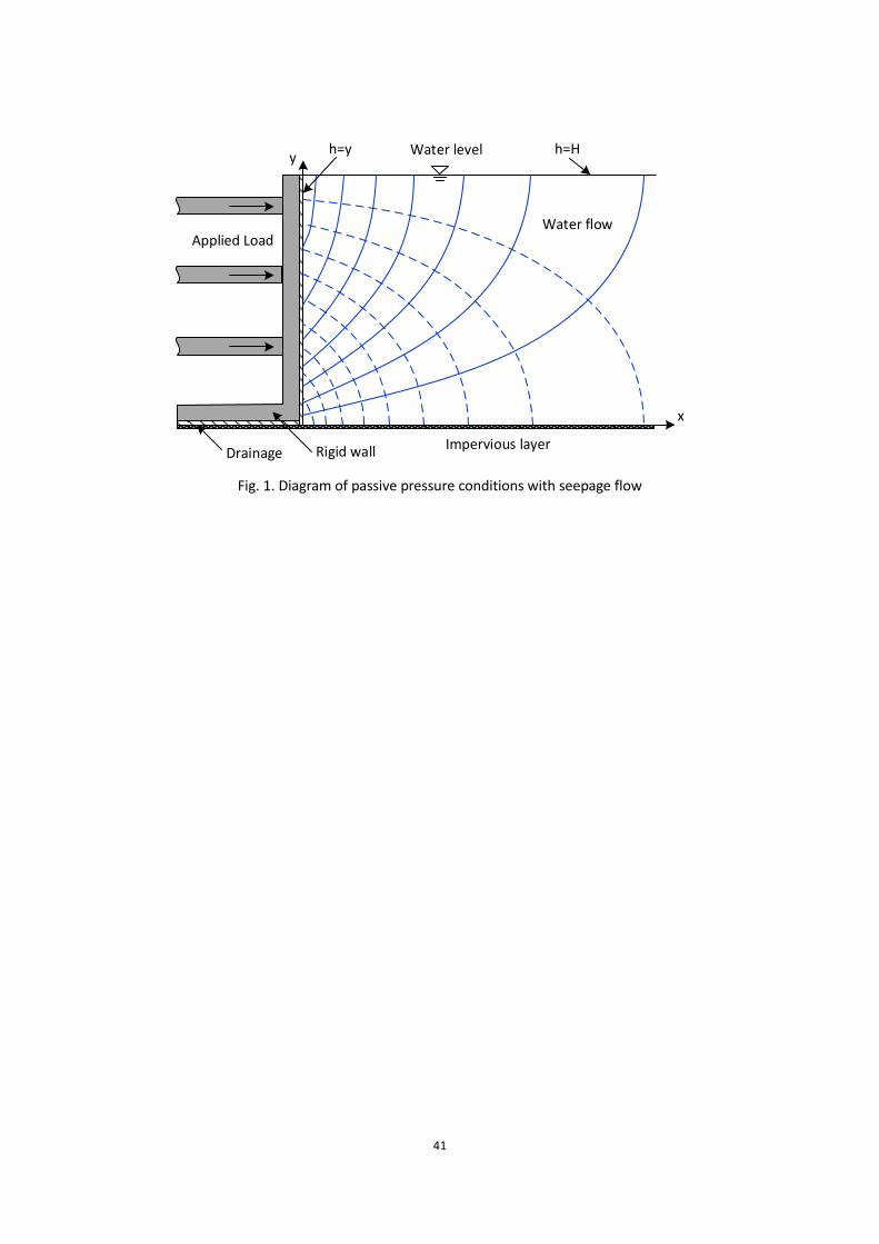
Assumptions 120
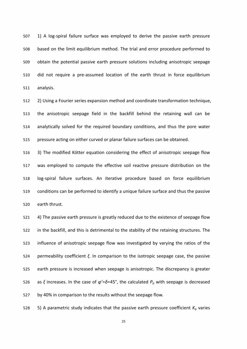
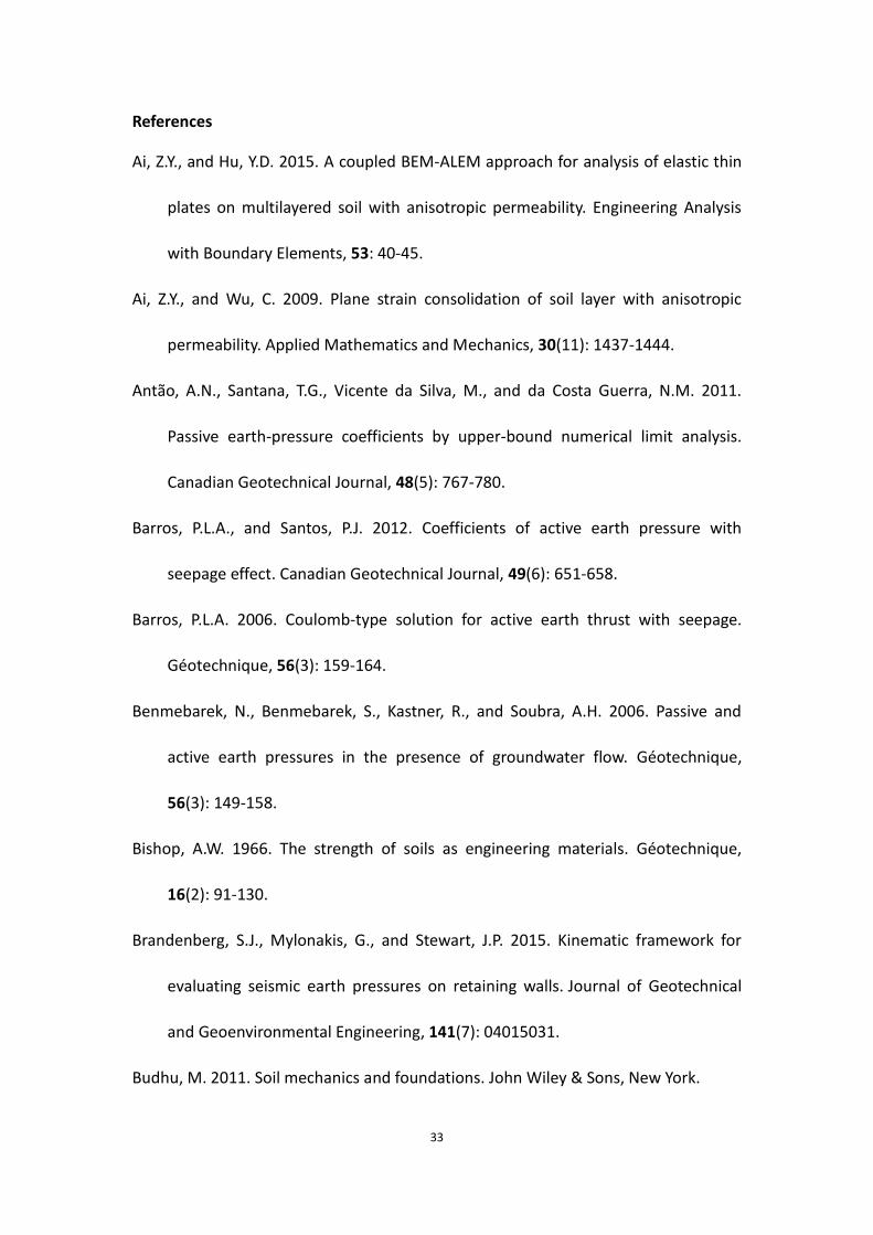
The analysis presented in this paper considers the case of a vertical rigid retaining 121
wall resting against a horizontal cohesionless backfill with anisotropic seepage flow, 122
originating from a continuous source on the horizontal surface. An external strut 123
force is pushing the wall to move towards the soil and the soil to behave passively. In 124
addition, the rigid retaining wall is provided with a drainage system along the 125
soil-wall interface and the layer beneath the wall. The horizontal surface at y=0 is an 126
impervious layer. The resulting flow net under anisotropic seepage conditions is 127
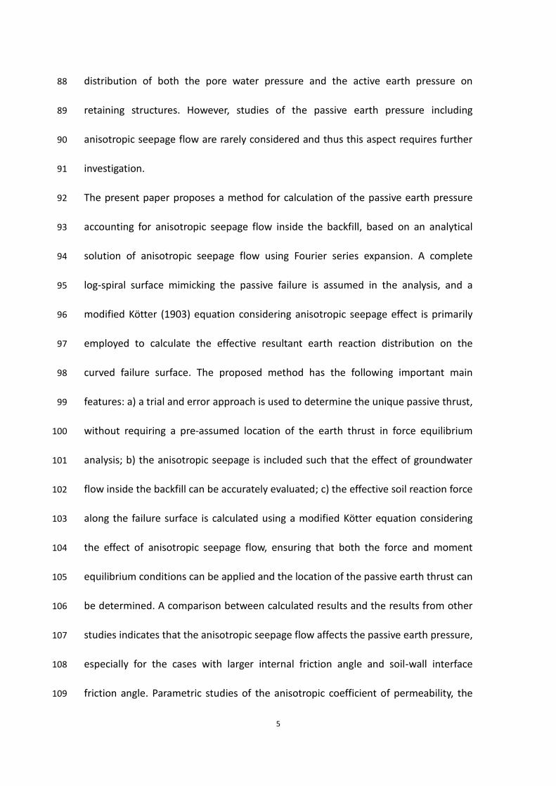
illustrated in Fig. 1. 128
In order to obtain the earth pressure solution given anisotropic seepage, the 129
following assumptions are made: 130
1) The shape of the failure surface is taken as a complete log spiral, extending from 131
7
the wall heel to the horizontal ground surface (Fig. 2). 132
2) The backfill is fully saturated and homogeneous, and the principal directions of 133
permeability coincide with the horizontal and vertical directions; 134
3) The flow is in the steady laminar state and obeys the linear form of Darcy’s law. 135
These assumptions have been widely used for the analysis of passive earth pressure 136
on retaining walls, e.g. Morrison and Ebeling (1995), Soubra and Macuh (2002), and 137
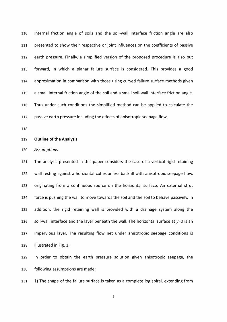
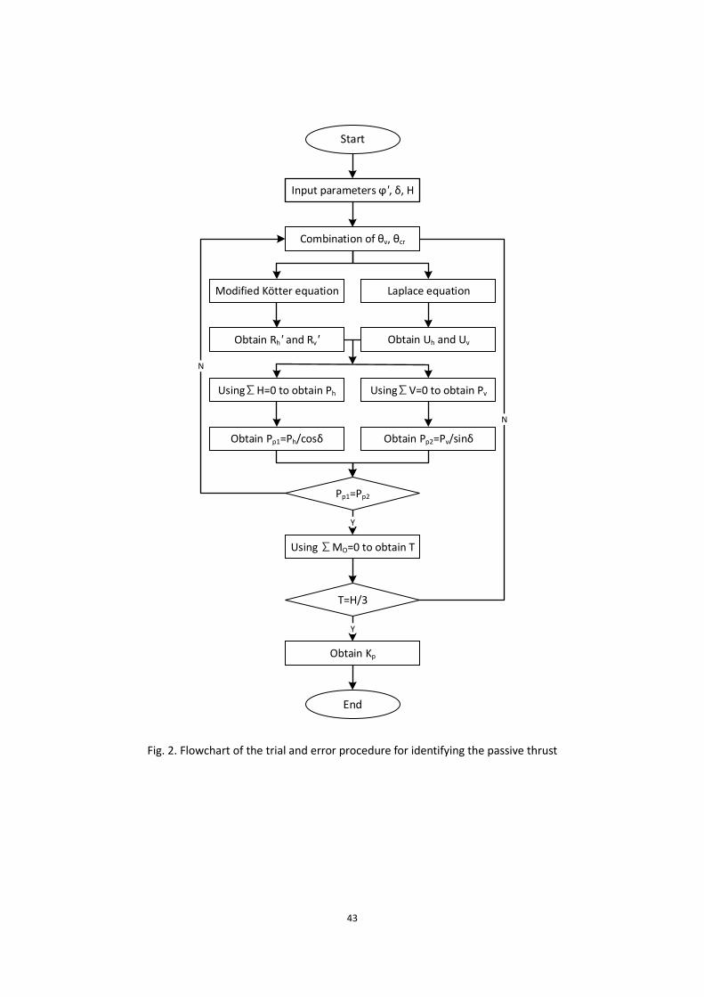
Patki et al. (2015a). 138
Methodology 139
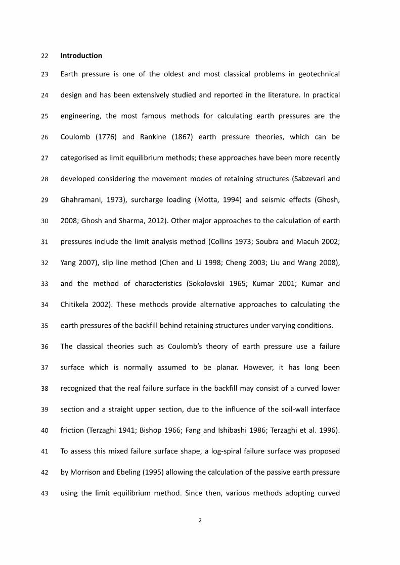
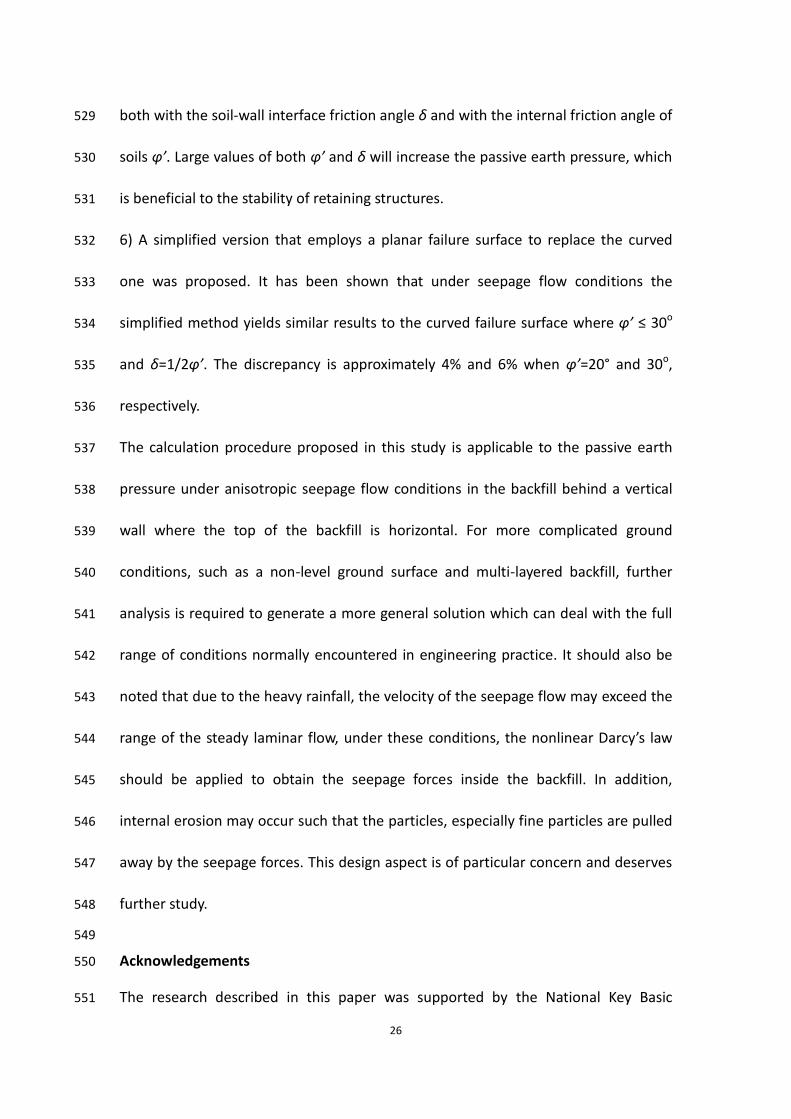
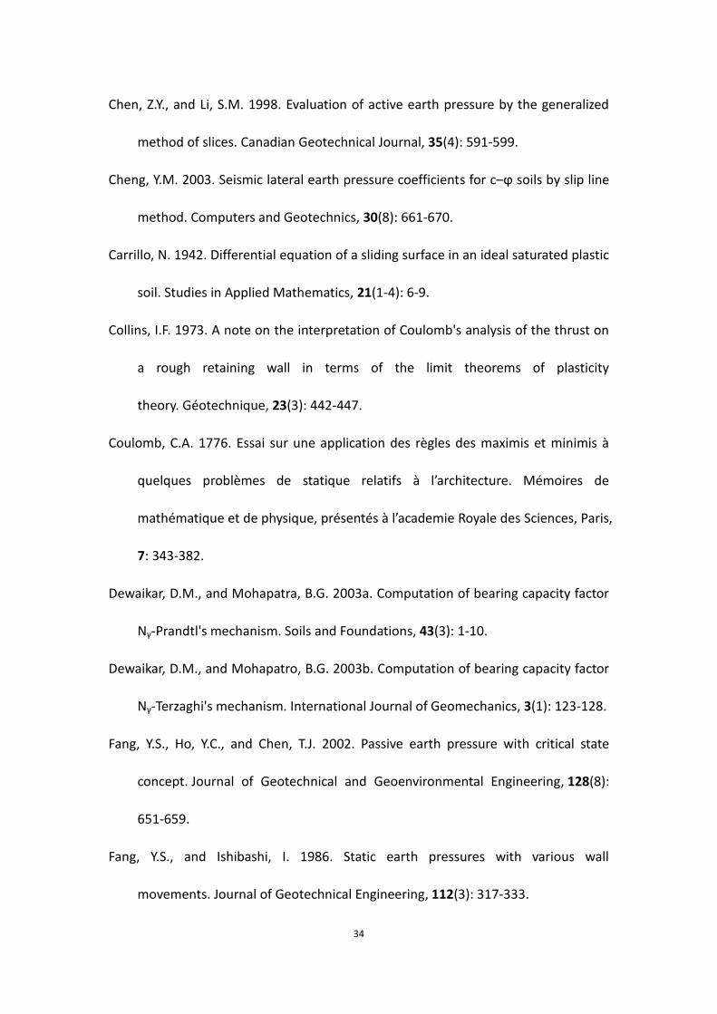
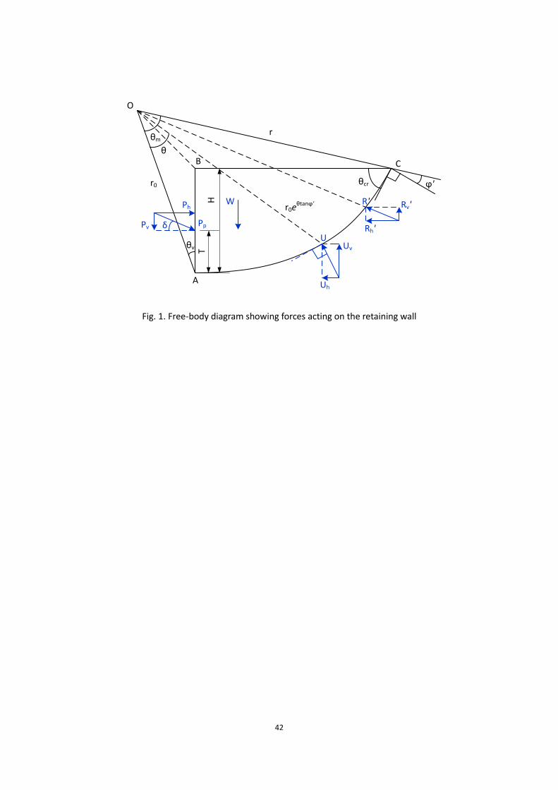
According to the free-body diagram of the failure wedge illustrated in Fig. 2, the 140
following forces are identified: 141
1) The passive thrust on the retaining wall Pp, of which the horizontal and vertical 142
components are Ph and Pv, respectively. 143
2) The self-weight of the failure segment ABC is W. 144
3) The effective resultant soil reaction force R’ along the failure surface AC. Its 145
horizontal and vertical components are designated as Rh’ and Rv’, respectively. 146
4) The resultant pore pressure force U, due to the seepage inside the backfill acting 147
on the failure surface AC. Its horizontal and vertical components are designated as 148
Uh and Uv, respectively. 149
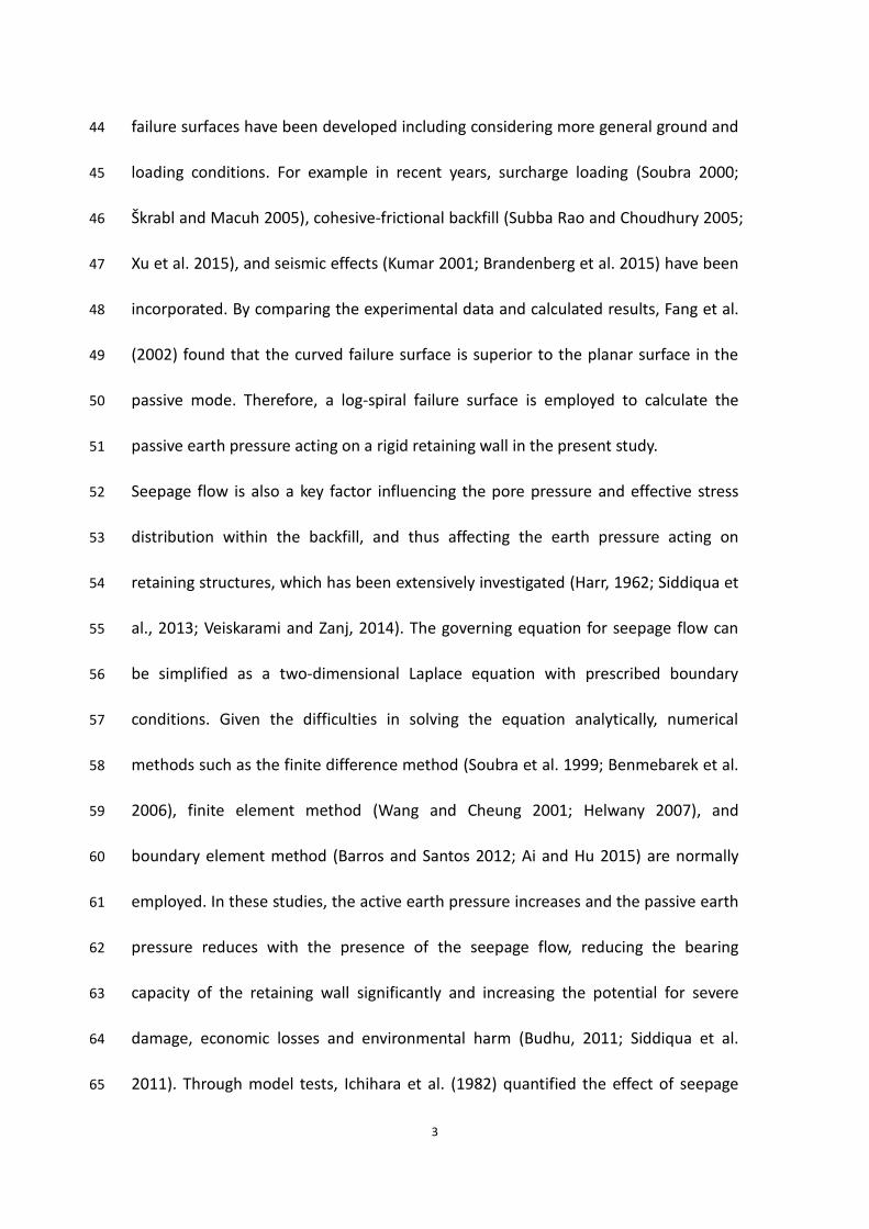
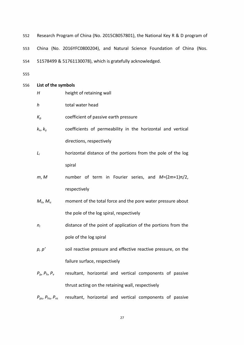
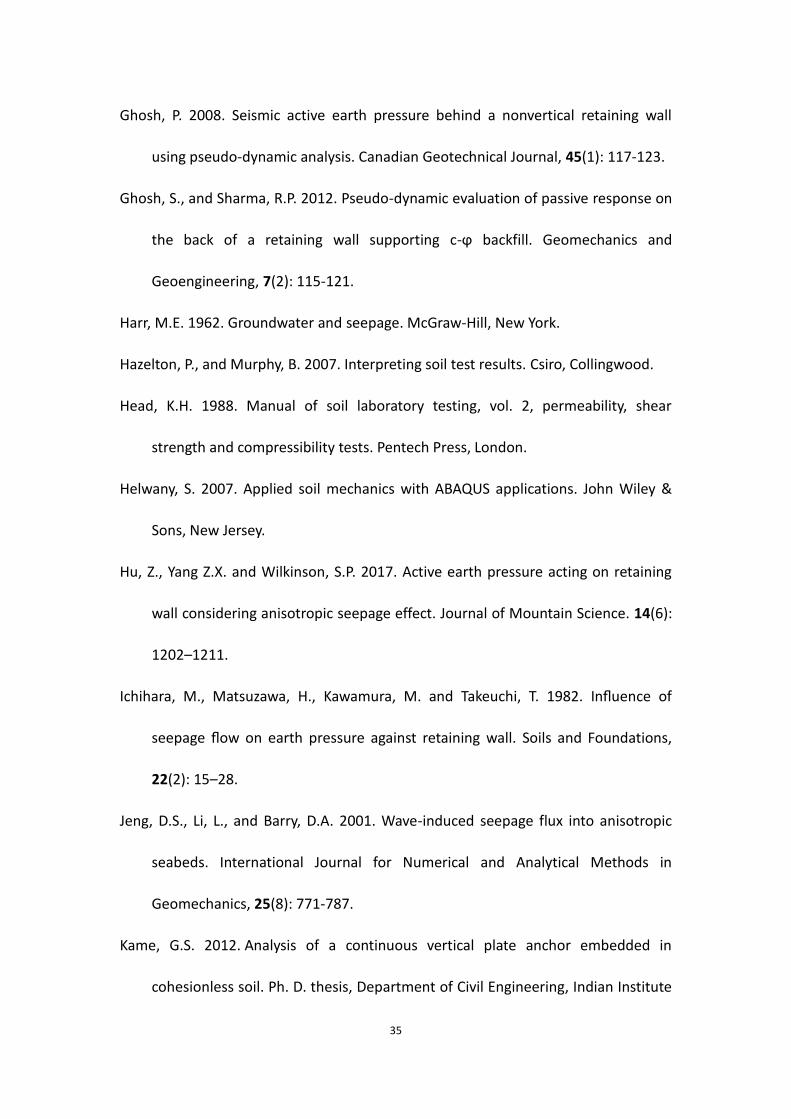
A trial and error procedure is performed to obtain the passive thrust Pp, following the 150
method shown in Fig. 3. Two parameters ϑv and ϑcr that determine the location of 151
the pole of the log spiral and the geometry of the failure wedge are treated as 152
unknowns in the iterative analysis. For any given values of the angle ϑv and ϑcr, it is 153
8
possible to determine a complete geometry of the failure wedge that is sensitive to 154
the input parameters, including the effective friction angle φ’, soil-wall interface 155
friction angle δ and the wall height H. A modified Kötter equation considering the 156
effect of seepage flow is applied to calculate the effective reaction force R’ along the 157
curved failure surface, and the pore water pressure force U resulting from the 158
seepage flow is obtained by solving the Laplace equation under the prescribed 159
boundary conditions (Fig. 1). Details of the effective reaction force and the pore 160
water pressure force will be presented towards the end of this paper. 161
The protocol proposed here involves the application of both horizontal and vertical 162
limit-equilibrium conditions to determine the horizontal and vertical earth pressure 163
components Ph and Pv, and thus the passive earth thrust with Pp= Ph /cosδ= Pv /sinδ. 164
If the assumed values of ϑv and ϑcr are acceptable, then the obtained passive thrust 165
Pp from both the horizontal and vertical directions must be equal or within a small 166
error range. If this is not the case the values of the angle ϑv and ϑcr are modified, and 167
the calculation procedure is repeated until the above convergence condition has 168
been satisfied. 169
Several values of passive thrust that fulfill the above conditions can be obtained, with 170
passive thrusts locations which can be obtained through back-calculation using the 171
moment equilibrium condition with known values of Pp. The criterion of T/H=1/3 is 172
applied in order to identify the optimum value of Pp. Therefore, the failure surface 173
that yields the closest value to T/H=1/3 will be identified for the passive thrusts 174
locations. The same approach has also been adopted by Barros (2006) and Patki et al. 175
9
(2017). 176
177
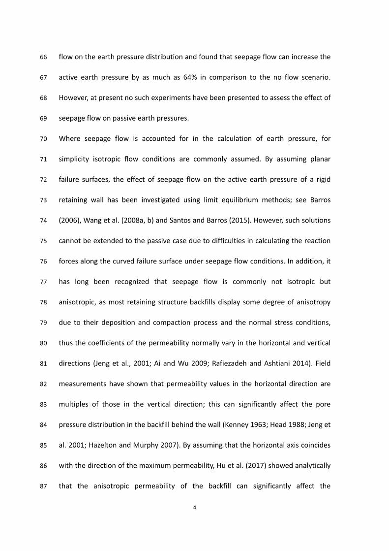
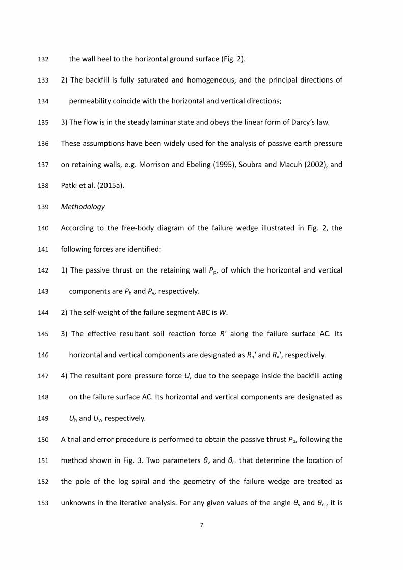
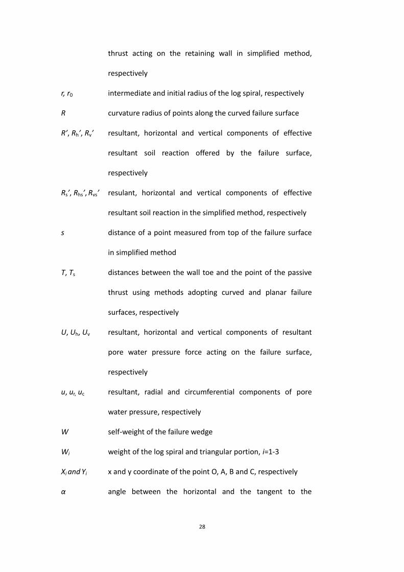
Anisotropic seepage solutions 178
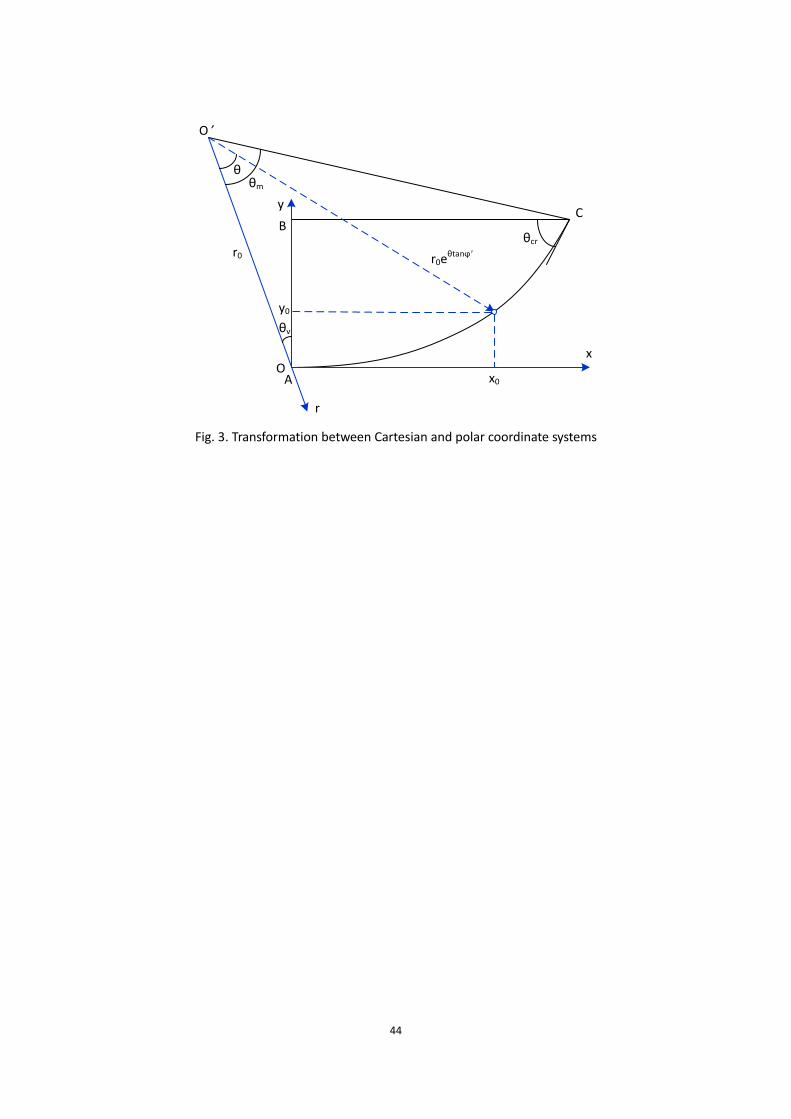
Total head h(x, y) 179
In the present study, seepage analysis is carried out primarily to determine the 2-D 180
distribution of the total head h(x, y). The mathematical model used to obtain the 181
solutions to the anisotropic seepage through the saturated backfill is derived from 182
the Laplace differential equation, 183
2 2
2 20x y
h hk k
x y
(1) 184
where kx and ky are coefficients of permeability in the horizontal and vertical 185
directions respectively. For the case considered in Fig. 1, Barros (2006) obtained a 186
solution to the Laplace equation for isotropic soil based on Fourier series expansion. 187
To investigate the effect of the anisotropy of seepage flow, the ratio of permeability 188
coefficient ξ=(ky/kx)1/2 was introduced by Hu et al. (2017), and the solution to the 189
Laplace equation for anisotropic seepage can be then obtained as 190
20
2( , ) 1 e cos
Mx
H
m
Myh x y H
M H
(2) 191
where m is number of term in Fourier series and M is obtained by 192
2 1
2
mM
(3) 193
The pore pressure at any point inside the soil mass is 194
, ,wu x y h x y y (4) 195
where γw is the unit weight of water. 196
In order to obtain the pore water pressure acting on the curved failure surface, the 197
10
total head h(x, y) along the log-spiral failure surface can be expressed in a polar 198
coordinate system, as shown in Fig. 4. The transformation equations between the x-y 199
Cartesian coordinate system and r-ϑ polar coordinates on the curved failure surface 200
can be obtained by 201
tan
0 0
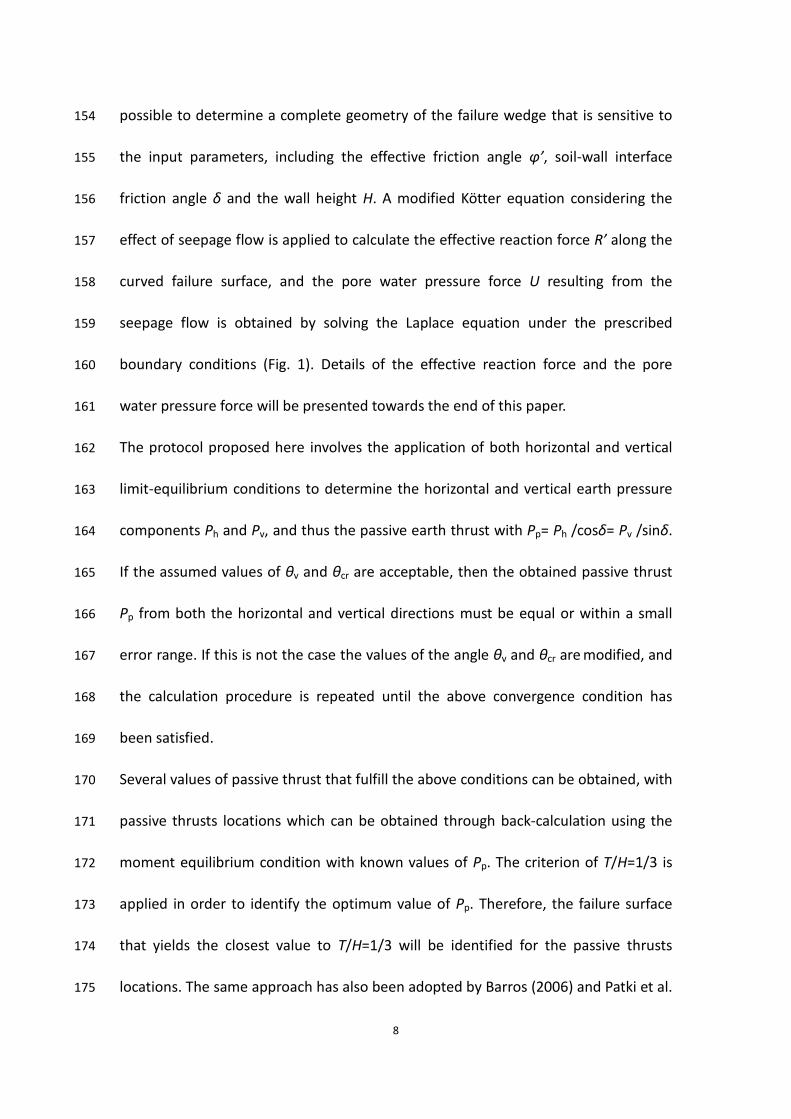
tan
0 0
sin e sin
cos e cos
'
v v
'
v v
x r r
y r r
(5) 202
where φ’ is the effective internal friction angle of soils, r0 is the initial radius of the 203
log spiral, ϑ is the angle made by the intermediate radii of the log spiral with the 204
initial radii. 205
Pore pressure along the curved failure surface 206
Based on the coordinate transformation rule given in Eq. (5), the total head along the 207
failure surface can be obtained, 208
tan
0 0sin sin tan
0 0
20
cos cos21 e cos
'v vM r r e '
v vH
m
M r r eh H
M H
(6) 209
thus, the pore pressure along the failure surface can be obtained, 210
tan
0 0cos e cos'
w v vu h r r (7) 211
Integration of Eq. (7) yields the resultant pore pressure force U along the curved 212
failure surface, which is given by 213
= dU u s (8) 214
In Eq. (8), u is the pore pressure acting perpendicular to the curved failure surface, 215
and its radial and circumferential components can be written as 216
r
c
cos
sin
u u '
u u '
(9) 217
The horizontal component of the resultant pore pressure force Uh is then obtained, 218
11
m m
m
tan tan
h r 0 c 00 0
tan
00
e sin sec d e cos sec d
e sin sec d
' '
v v
'
v
U u r ' u r '
ur ' '
(10) 219
Similarly, the vertical component Uv of the resultant pore pressure force is, 220
m m
m
tan tan
v r 0 c 00 0
tan
00
e cos sec d e sin sec d
e cos sec d
' '
v v
'
v
U u r ' u r '
ur ' '
(11) 221
As the radial component of pore pressure ur passes through the pole of the log-spiral, 222
its contribution to the moment equilibrium condition is null. Therefore, only the 223
moment of the circumferential pore pressure uc is contributed as 224
m mtan 2 2 tan 2 2 tan
u c 0 c 0 00 0
e d e sec d e tan d' ' 'M u r s u r ' ur '
(12) 225
226
Determination of passive earth pressure 227
Force equilibrium conditions can be applied to determine the passive earth thrust Pp, 228
where the weight of the failure wedge W, the effective reaction force R’ acting on the 229
failure surface, and the resultant pore pressure force U are all known. The calculation 230
procedure of W and R’ is presented below. From these parameters the passive earth 231
thrust Pp and its location of application can be obtained. 232
Weight of the failure wedge 233
Considering the log-spiral curved failure surface shown in Fig. 5, the weight of the 234
failure wedge W can be calculated by 235
1 2 3=W W W W (13) 236
in which W1 is the weight of the log spiral part OAC, W2 is the weight of the triangular 237
part OBC, and W3 is the weight of the triangular part OAB. W1, W2 and W3, can be 238
given below, 239
12
mm m
22
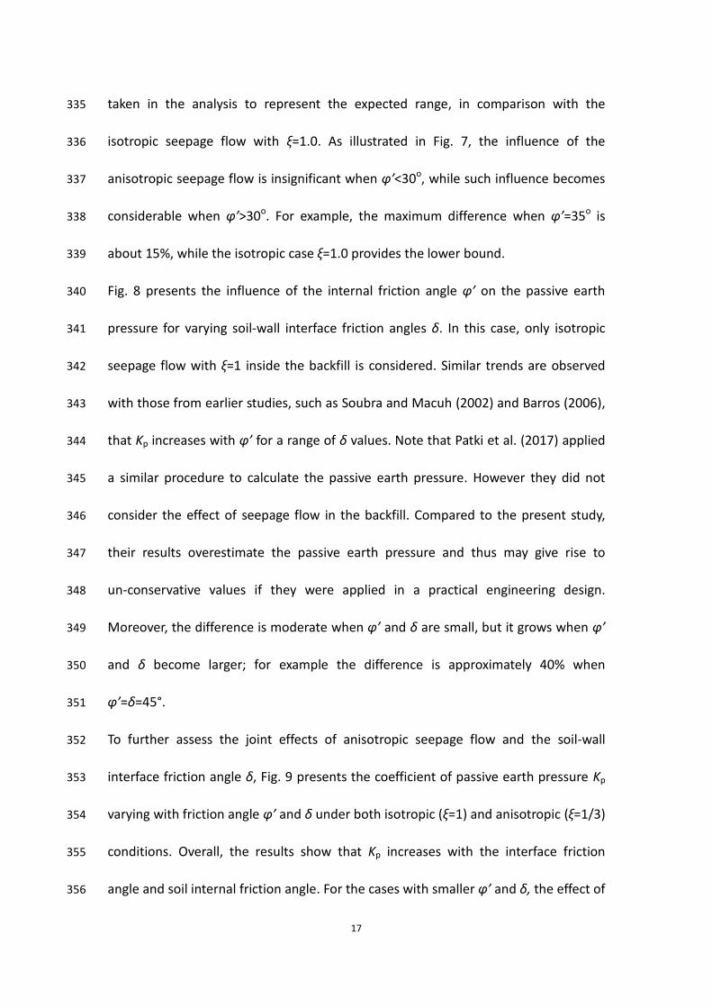
tan 2 tan0
1 sat 0 sat0
2 sat o b c b c o c o b
3 sat o a b a b o b o a
1 1= e d e 1
2 4 tan
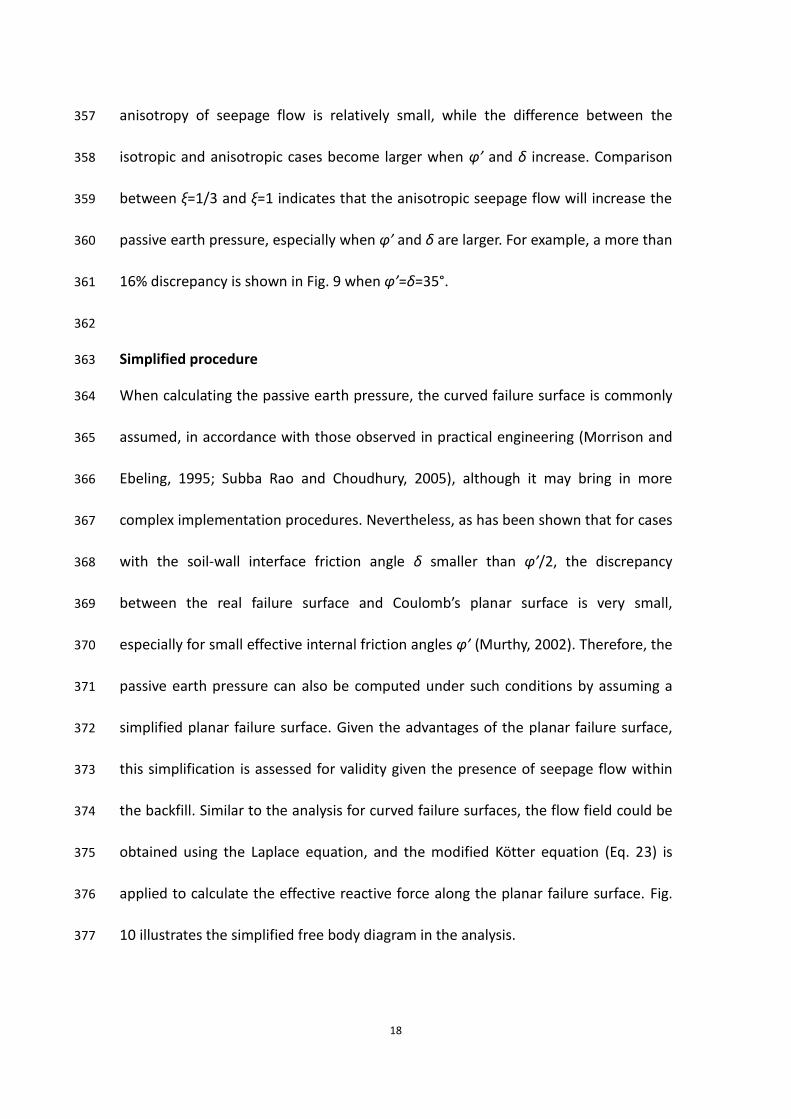
1=
2
1=
2
' 'rW r
W X Y Y X Y Y X Y Y
W X Y Y X Y Y X Y Y
(14) 240
where γsat is the unit weight of saturated soil, Xi and Yi are the x and y coordinates of 241
point i (i= O, A, B and C). 242
Xi and Yi can be determined with the known initial radius r0 (OA), the distances OB 243
and OC, which can be calculated by 244
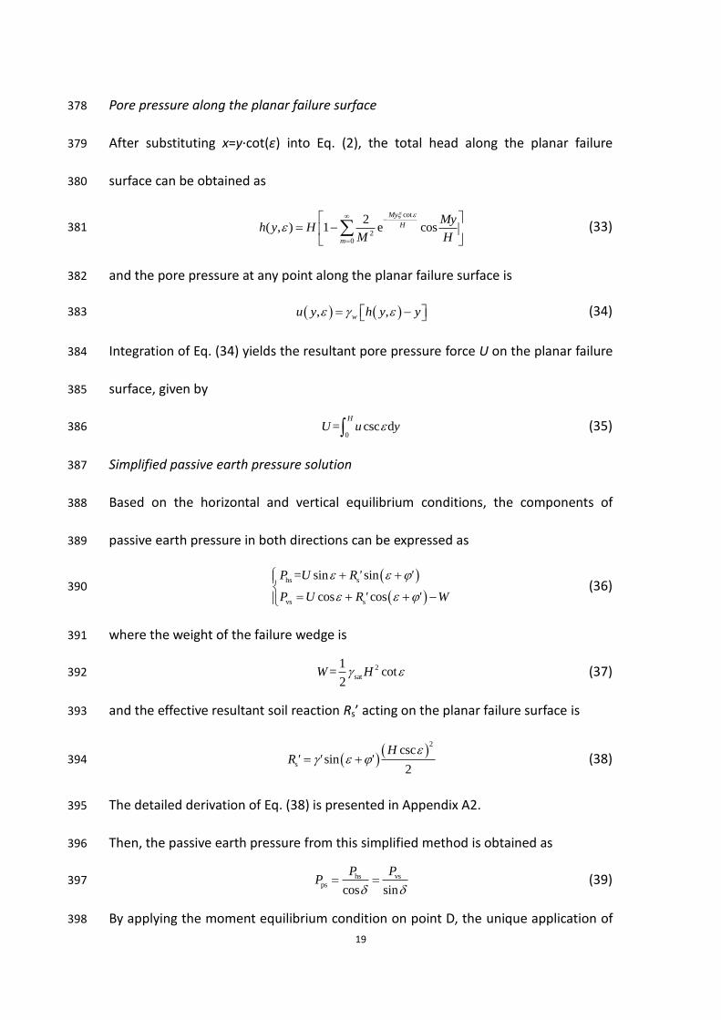
m
0
tan
0
cos
cos
sin
cos
e
v
v
v
'
HOA r
HOB
OC r
(15) 245
where β is the angle between OB and the horizontal direction calculated by 246
m tan
cr1e cos
= tansin
'
v
'
(16) 247
Solution of the modified Kötter equation 248
For the cohesionless homogeneous soil under passive state, the distribution of soil 249
reaction along the curved failure surface can be obtained by original Kötter (1903) 250
equation (Fig. 6), which can be written as, 251
2 tan sin 0p
ps s
(17) 252
where α is the tangential angle at the differential point on the failure surface with 253
respect to the horizontal axis; γ is the unit weight of soils. 254
Dewaikar and Mohapatra (2003a, b) applied the Kötter (1903) equation to the limit 255
13
equilibrium analysis of shallow foundation bearing capacity problems, which has also 256
been applied to earth pressure problems by Kame (2012) and Patki et al. (2015b, 257
2017). Note that these studies are restricted to the conditions without seepage flow. 258
By considering the effect of seepage flow in the backfill, the Kötter equation can be 259
modified into (Carrillo 1942): 260
sat2 tan sin cos sin 0p' u u
p' ' ' ' 's s s R
(18) 261
or 262
sat2 tan sin cos sin 0p' u u
p' ' R ' ' R 'R
(19) 263
where R is the curvature radius along the curved failure surface. 264
In a polar coordinate system with x=R·sinα and y=H-R·cosα, the total head of water h 265
can be expressed as 266
cosw
uh H R
(20) 267
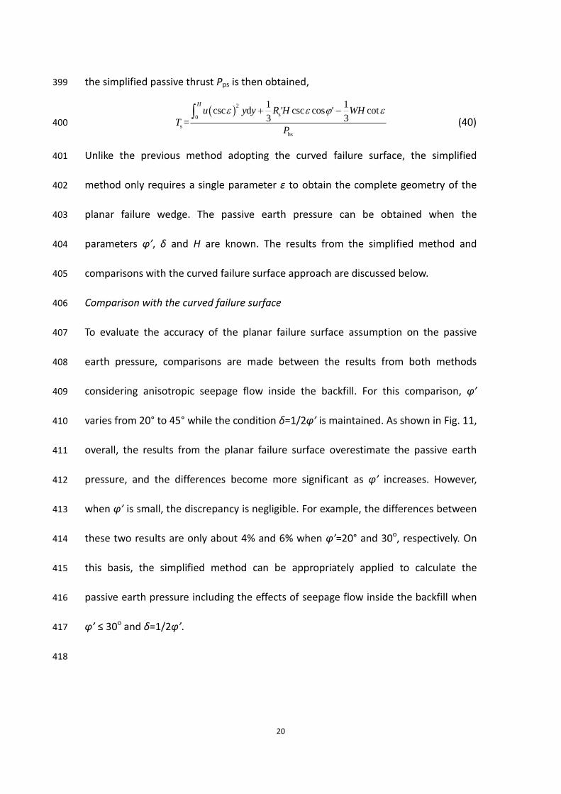
The derivatives of pore water pressure u with respect to α and R can then be 268
obtained as 269
sin
cos
w
w
u hR
u h
R R
(21) 270
Substituting Eq. (21) into Eq. (19), the modified Kötter equation can be written into 271
sat2 tan sin sin cos cos sin 0w w
p' h hp' ' R ' R ' R '
R
(22) 272
or 273
sat
Buoyancy effectSeepage effect
2 tan sin cos sin 0w w
p' h hp' ' R ' ' R '
R
(23) 274
As seen in Eq. (23), the effect caused by the presence of water has two parts, i.e. 275
14
buoyancy force and seepage force. For the special case of saturated soil without 276
seepage inside the backfill or a planar failure surface concerned, the solution to Eq. 277
(23) can be analytically obtained, as described in Appendix A. However, for the case 278
with a log-spiral failure surface considering seepage effect, there is no analytical 279
solution to the modified Kötter equation expressed in Eq. (23). Instead, a numerical 280
procedure based on Runge-Kutta method was applied to solve the modified Kötter 281
equation using the commercial software MATLAB. The effective reactive pressure p’ 282
under given boundary conditions can thus be obtained. 283
The total reactive pressure p along the failure surface is then obtained by summing 284
up the effective pressure p’ and pore water pressure u. The integration of Eq. (23) 285
gives the effective reactive pressure distribution, and double integration yields the 286
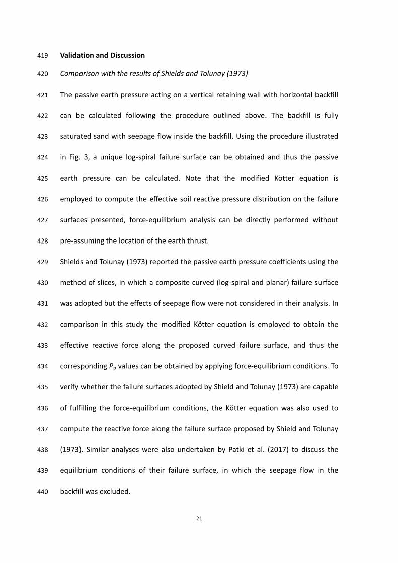
effective resultant soil reaction R’ on the log-spiral failure surface. Therefore, the 287
horizontal and vertical components of the effective resultant soil reaction are given 288
by 289
m
m
tan
h 00
tan
v 00
e sin sec d
e cos sec d
'
v
'
v
R ' p'r '
R ' p'r '
(24) 290
Passive earth pressure solution 291
The passive earth pressure acting on the retaining wall can be obtained using force 292
equilibrium conditions in both the horizontal and vertical directions. Considering the 293
horizontal force equilibrium illustrated in Fig. 2, the horizontal component of the 294
passive earth thrust can be expressed as 295
h h hP R ' U (25) 296
15
Similarly, vertical force equilibrium gives the vertical component as 297
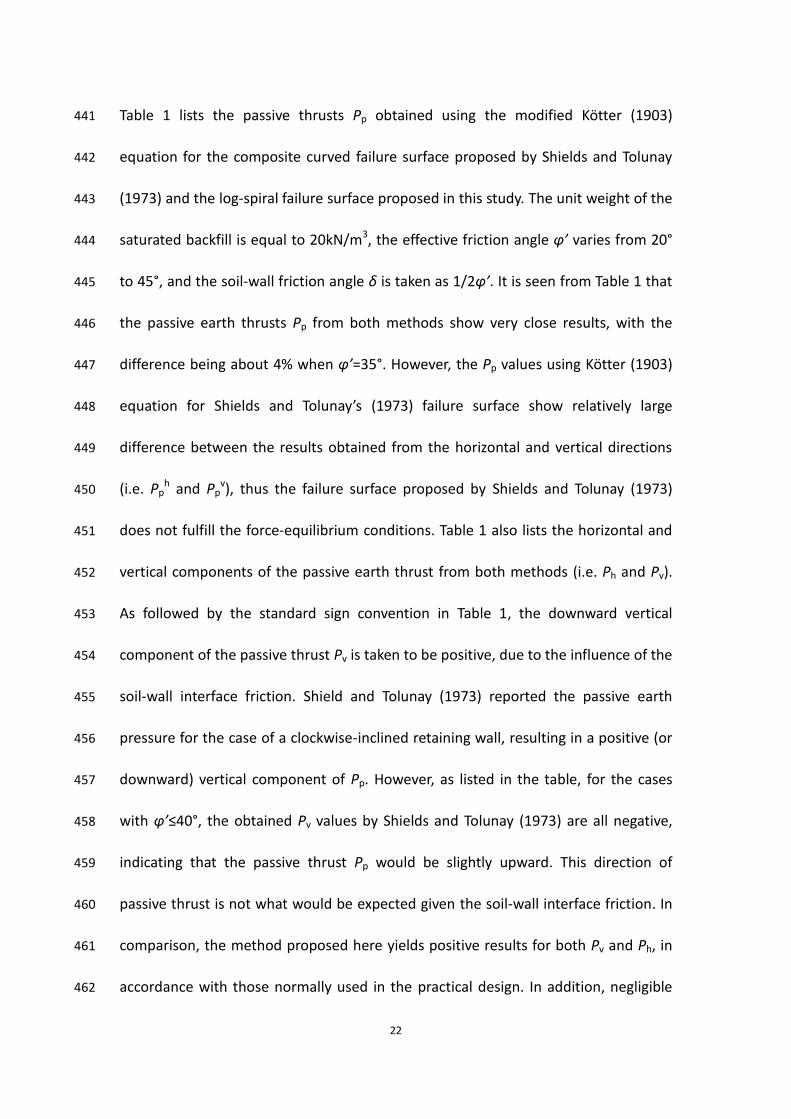
v v vP U R ' W (26) 298
Combining Eqs. (25) and (26) yields 299
h h hp
cos cos
P R ' UP
(27) 300
or 301
v v v
psin sin
P U R ' WP
(28) 302
As illustrated in the flowchart in Fig. 3, the iterative procedure can be repeated until 303
the discrepancy between the two values of Pp is within a prescribed tolerance, which 304
is set as 0.1% of the mean value of Pp obtained using Eqs. (27) and (28) in the present 305
study. 306
Location of the passive thrust 307
Considering the moment equilibrium condition on the pole of the log spiral O, the 308
distance T is then obtained by 309
1 1 2 2 3 3 u v
v
h
cos= cos
W L W L W L M P OBT OA
P
(29) 310
where L1, L2 and L3 are the horizontal distances between the centers of gravity of OAC, 311
OBC and OAB and point O, respectively, as shown in Fig. 5, and can be obtained by 312
1 1 v 2 v
o b c
2
o a b
3
cos sin
=3
=3
L n n
X X XL
X X XL
(30) 313
where 314
16
m
m
m
m
3 tan
m m0
1 2 tan2
3 tan
m m0
2 2 tan2
e sin 3tan cos 3tan4 tan
e 13 1 9 tan
1 e cos 3tan sin4 tan
e 13 1 9 tan
'
'
'
'
' 'r 'n
'
'r 'n
'
(31) 315
As indicated in the flowchart (Fig. 3), several passive thrusts Pp can be obtained that 316
satisfy the conditions set out in this study, while the locations of Pp may vary. It has 317
been shown that in most cases, the application of the passive thrust Pp is located at 318
1/3H, which yields the optimum result (Barros 2006; Xu et al. 2015; Patki et al. 2017). 319
Therefore, the 1/3H criterion is adopted for selecting the optimum passive thrust Pp, 320
and from this the coefficient of passive earth pressure considering seepage flow Kp 321
can be obtained, 322
p
p 2
sat
2PK
H (32) 323
Parametric analysis 324
Some of the key parameters that may influence the passive earth pressure including 325
the ratio of permeability coefficient ξ, the effective friction angle φ’ and the soil-wall 326
interface friction angle δ are considered during the parametric analysis. Fig. 7 327
presents the influence of anisotropic seepage flow on the coefficient of passive earth 328
pressure Kp, in which φ’ varies within the range of 20o–45o while the condition 329
δ=1/2φ’ is maintained. It is noted that the value of the ratio of permeability 330
coefficient ξ is assumed to vary from 0 to 1, as the horizontal permeability coefficient 331
is normally greater than the vertical (kx/ky > 1) in normal sedimentary deposits as 332
well as the backfill behind the retaining walls (Taylor 1948; Harr 1962; Kenny 1963; 333
Head 1988; Rafiezadeh and Ashtiani 2014). Three values of ξ (=1/3, 1/2 and 2/3) are 334
17
taken in the analysis to represent the expected range, in comparison with the 335
isotropic seepage flow with ξ=1.0. As illustrated in Fig. 7, the influence of the 336
anisotropic seepage flow is insignificant when φ’<30o, while such influence becomes 337
considerable when φ’>30o. For example, the maximum difference when φ’=35o is 338
about 15%, while the isotropic case ξ=1.0 provides the lower bound. 339
Fig. 8 presents the influence of the internal friction angle φ’ on the passive earth 340
pressure for varying soil-wall interface friction angles δ. In this case, only isotropic 341
seepage flow with ξ=1 inside the backfill is considered. Similar trends are observed 342
with those from earlier studies, such as Soubra and Macuh (2002) and Barros (2006), 343
that Kp increases with φ’ for a range of δ values. Note that Patki et al. (2017) applied 344
a similar procedure to calculate the passive earth pressure. However they did not 345
consider the effect of seepage flow in the backfill. Compared to the present study, 346
their results overestimate the passive earth pressure and thus may give rise to 347
un-conservative values if they were applied in a practical engineering design. 348
Moreover, the difference is moderate when φ’ and δ are small, but it grows when φ’ 349
and δ become larger; for example the difference is approximately 40% when 350
φ’=δ=45°. 351
To further assess the joint effects of anisotropic seepage flow and the soil-wall 352
interface friction angle δ, Fig. 9 presents the coefficient of passive earth pressure Kp 353
varying with friction angle φ’ and δ under both isotropic (ξ=1) and anisotropic (ξ=1/3) 354
conditions. Overall, the results show that Kp increases with the interface friction 355
angle and soil internal friction angle. For the cases with smaller φ’ and δ, the effect of 356
18
anisotropy of seepage flow is relatively small, while the difference between the 357
isotropic and anisotropic cases become larger when φ’ and δ increase. Comparison 358
between ξ=1/3 and ξ=1 indicates that the anisotropic seepage flow will increase the 359
passive earth pressure, especially when φ’ and δ are larger. For example, a more than 360
16% discrepancy is shown in Fig. 9 when φ’=δ=35°. 361
362
Simplified procedure 363
When calculating the passive earth pressure, the curved failure surface is commonly 364
assumed, in accordance with those observed in practical engineering (Morrison and 365
Ebeling, 1995; Subba Rao and Choudhury, 2005), although it may bring in more 366
complex implementation procedures. Nevertheless, as has been shown that for cases 367
with the soil-wall interface friction angle δ smaller than φ’/2, the discrepancy 368
between the real failure surface and Coulomb’s planar surface is very small, 369
especially for small effective internal friction angles φ’ (Murthy, 2002). Therefore, the 370
passive earth pressure can also be computed under such conditions by assuming a 371
simplified planar failure surface. Given the advantages of the planar failure surface, 372
this simplification is assessed for validity given the presence of seepage flow within 373
the backfill. Similar to the analysis for curved failure surfaces, the flow field could be 374
obtained using the Laplace equation, and the modified Kötter equation (Eq. 23) is 375
applied to calculate the effective reactive force along the planar failure surface. Fig. 376
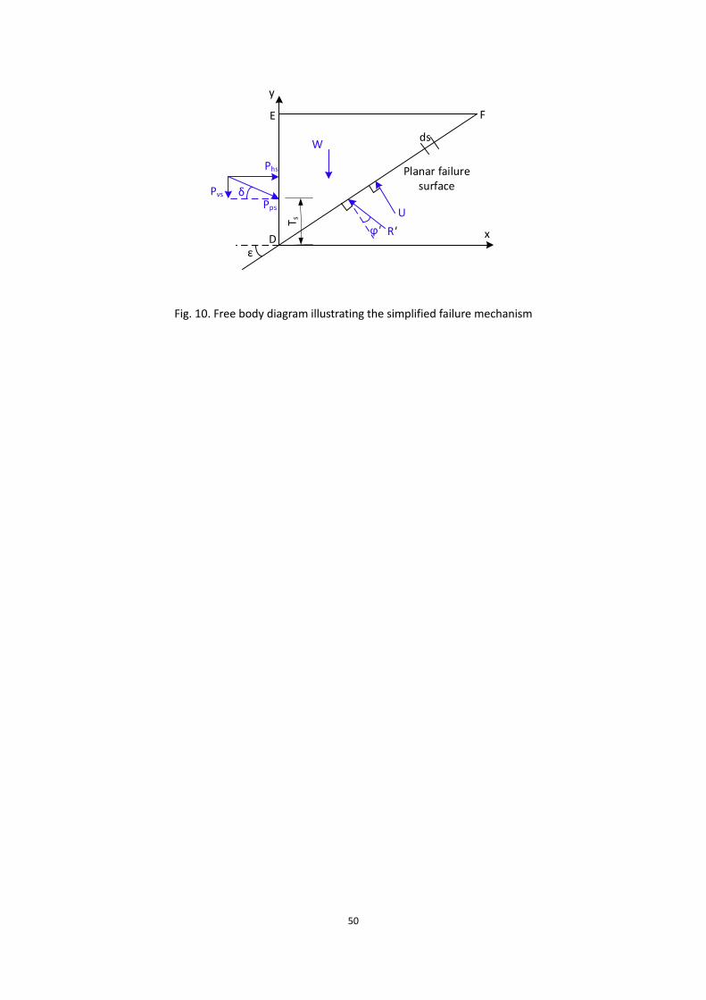
10 illustrates the simplified free body diagram in the analysis. 377
19
Pore pressure along the planar failure surface 378
After substituting x=y·cot(ε) into Eq. (2), the total head along the planar failure 379
surface can be obtained as 380
cot
20
2( , ) 1 e cos
My
H
m
Myh y H
M H
(33) 381
and the pore pressure at any point along the planar failure surface is 382
, ,wu y h y y (34) 383
Integration of Eq. (34) yields the resultant pore pressure force U on the planar failure 384
surface, given by 385
0
= csc dH
U u y (35) 386
Simplified passive earth pressure solution 387
Based on the horizontal and vertical equilibrium conditions, the components of 388
passive earth pressure in both directions can be expressed as 389
hs s
vs s
= sin sin
cos cos
P U R' '
P U R' ' W
(36) 390
where the weight of the failure wedge is 391
2
sat
1= cot
2W H (37) 392
and the effective resultant soil reaction Rs’ acting on the planar failure surface is 393
2
s
cscsin
2
HR' ' '
(38) 394
The detailed derivation of Eq. (38) is presented in Appendix A2. 395
Then, the passive earth pressure from this simplified method is obtained as 396
hs vs
pscos sin
P PP
(39) 397
By applying the moment equilibrium condition on point D, the unique application of 398
20
the simplified passive thrust Pps is then obtained, 399
2
s0
s
hs
1 1csc d csc cos cot
3 3=
H
u y y R 'H ' WH
TP
(40) 400
Unlike the previous method adopting the curved failure surface, the simplified 401
method only requires a single parameter ε to obtain the complete geometry of the 402
planar failure wedge. The passive earth pressure can be obtained when the 403
parameters φ’, δ and H are known. The results from the simplified method and 404
comparisons with the curved failure surface approach are discussed below. 405
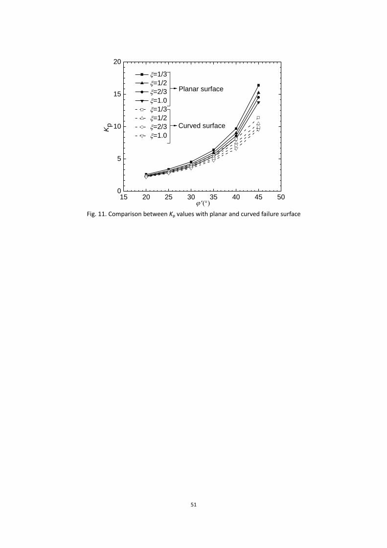
Comparison with the curved failure surface 406
To evaluate the accuracy of the planar failure surface assumption on the passive 407
earth pressure, comparisons are made between the results from both methods 408
considering anisotropic seepage flow inside the backfill. For this comparison, φ’ 409
varies from 20° to 45° while the condition δ=1/2φ’ is maintained. As shown in Fig. 11, 410
overall, the results from the planar failure surface overestimate the passive earth 411
pressure, and the differences become more significant as φ’ increases. However, 412
when φ’ is small, the discrepancy is negligible. For example, the differences between 413
these two results are only about 4% and 6% when φ’=20° and 30o, respectively. On 414
this basis, the simplified method can be appropriately applied to calculate the 415
passive earth pressure including the effects of seepage flow inside the backfill when 416
φ’ ≤ 30o and δ=1/2φ’. 417
418
21
Validation and Discussion 419
Comparison with the results of Shields and Tolunay (1973) 420
The passive earth pressure acting on a vertical retaining wall with horizontal backfill 421
can be calculated following the procedure outlined above. The backfill is fully 422
saturated sand with seepage flow inside the backfill. Using the procedure illustrated 423
in Fig. 3, a unique log-spiral failure surface can be obtained and thus the passive 424
earth pressure can be calculated. Note that the modified Kötter equation is 425
employed to compute the effective soil reactive pressure distribution on the failure 426
surfaces presented, force-equilibrium analysis can be directly performed without 427
pre-assuming the location of the earth thrust. 428
Shields and Tolunay (1973) reported the passive earth pressure coefficients using the 429
method of slices, in which a composite curved (log-spiral and planar) failure surface 430
was adopted but the effects of seepage flow were not considered in their analysis. In 431
comparison in this study the modified Kötter equation is employed to obtain the 432
effective reactive force along the proposed curved failure surface, and thus the 433
corresponding Pp values can be obtained by applying force-equilibrium conditions. To 434
verify whether the failure surfaces adopted by Shield and Tolunay (1973) are capable 435
of fulfilling the force-equilibrium conditions, the Kötter equation was also used to 436
compute the reactive force along the failure surface proposed by Shield and Tolunay 437
(1973). Similar analyses were also undertaken by Patki et al. (2017) to discuss the 438
equilibrium conditions of their failure surface, in which the seepage flow in the 439
backfill was excluded. 440
22
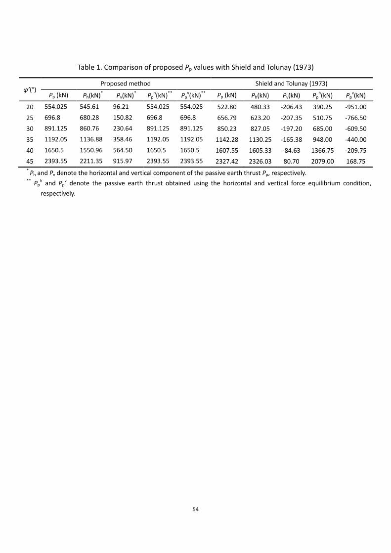
Table 1 lists the passive thrusts Pp obtained using the modified Kötter (1903) 441
equation for the composite curved failure surface proposed by Shields and Tolunay 442
(1973) and the log-spiral failure surface proposed in this study. The unit weight of the 443
saturated backfill is equal to 20kN/m3, the effective friction angle φ’ varies from 20° 444
to 45°, and the soil-wall friction angle δ is taken as 1/2φ’. It is seen from Table 1 that 445
the passive earth thrusts Pp from both methods show very close results, with the 446
difference being about 4% when φ’=35°. However, the Pp values using Kötter (1903) 447
equation for Shields and Tolunay’s (1973) failure surface show relatively large 448
difference between the results obtained from the horizontal and vertical directions 449
(i.e. Pph and Pp
v), thus the failure surface proposed by Shields and Tolunay (1973) 450
does not fulfill the force-equilibrium conditions. Table 1 also lists the horizontal and 451
vertical components of the passive earth thrust from both methods (i.e. Ph and Pv). 452
As followed by the standard sign convention in Table 1, the downward vertical 453
component of the passive thrust Pv is taken to be positive, due to the influence of the 454
soil-wall interface friction. Shield and Tolunay (1973) reported the passive earth 455
pressure for the case of a clockwise-inclined retaining wall, resulting in a positive (or 456
downward) vertical component of Pp. However, as listed in the table, for the cases 457
with φ’≤40°, the obtained Pv values by Shields and Tolunay (1973) are all negative, 458
indicating that the passive thrust Pp would be slightly upward. This direction of 459
passive thrust is not what would be expected given the soil-wall interface friction. In 460
comparison, the method proposed here yields positive results for both Pv and Ph, in 461
accordance with those normally used in the practical design. In addition, negligible 462
23
discrepancies are observed between the results of Pph and Pp
v, indicating that the 463
failure mechanism adopted in this study fulfills the force equilibrium conditions with 464
the criterion of the passive thrust Pp located at 1/3H of the retaining wall. 465
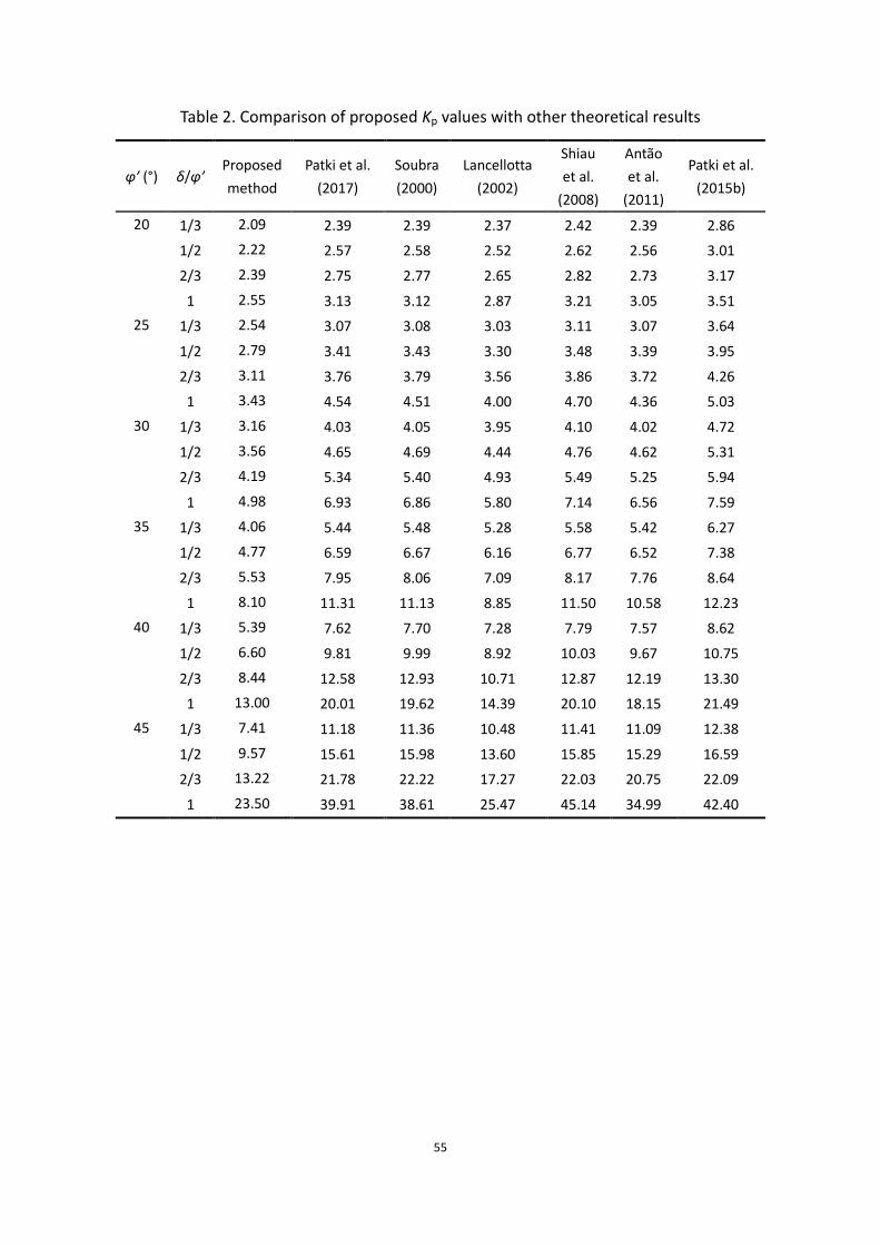
Comparison with other theoretical results 466
To further assess the effects of seepage flow on the passive earth pressure, Table 2 467
presents the comparisons of Kp values between the present study and other methods 468
reported in the literature, including Soubra (2000), Shiau et al. (2008), Antão et al. 469
(2011), Lancellotta (2002), and Patki et al. (2015b, 2017). Only isotropic seepage flow 470
with ξ=1 is considered herein. The same ranges of the parameters as those in Table 1 471
are considered for a vertical retaining wall resting against a horizontal cohesionless 472
backfill, while the effects of seepage flow were not taken into account in their 473
analyses. Note that Soubra (2000) used the limit analysis method considering the 474
kinematic conditions to obtain the upper-bound solutions of the passive earth 475
pressure. Shiau et al. (2008) and Antão et al. (2011) adopted the limit analysis 476
coupled with the finite element method, and obtained the upper-bound solutions of 477
passive earth pressure. In comparison, Lancellotta (2002) proposed an analytical 478
lower-bound solution based on the limit analysis method. The limit equilibrium 479
method coupled with the original Kötter equation was employed by Patki et al. 480
(2015b, 2017), with the former adopting the composite failure surface comprising a 481
log spiral followed by its tangent and the latter adopting the complete log-spiral 482
failure surface. The resultant earth reaction distributing on the curved failure surface 483
was directly obtained by solving the original Kötter equation. 484
24
As seen in Table 2, the Kp values using the proposed method employing the log-spiral 485
failure surface are in fairly good agreements with the theoretical results from the 486
studies outlined above. Because the method proposed in this study accounts for 487
seepage flow effects, it yields smaller Kp values than those obtained by the other 488
methods, as evidenced by Table 2. It is also noted that the discrepancy grows as φ’ 489
and δ increase; for example it could be 10–40% lower than the results obtained by 490
Patki et al. (2017), which is a special case of the proposed method if seepage flow is 491
not addressed in the backfill. 492
It is worth noting that the passive earth thrust is regarded as the main supporting 493
force ensuring the stability of the retaining structures in design. When there exists 494
the seepage flow inside the backfill, the passive earth pressures will be decreased, 495
and the ultimate capacity of the retaining structure will be reduced, leading to the 496
potential for instability problems during the retaining walls design life. In such cases, 497
it is of vital importance to account for the effects of seepage flow during design 498
calculations. 499
500
Conclusions 501
This paper presents an analytical procedure to calculate the passive earth pressure 502
acting on a retaining wall, considering the anisotropic seepage flow through a 503
cohesionless backfill. The main focus of this paper is the effect of anisotropic seepage 504
flow on the passive earth pressure, when applied to more realistic failure surfaces. 505
The conclusions of this work are summarized below: 506
25
1) A log-spiral failure surface was employed to derive the passive earth pressure 507
based on the limit equilibrium method. The trial and error procedure performed to 508
obtain the potential passive earth pressure solutions including anisotropic seepage 509
did not require a pre-assumed location of the earth thrust in force equilibrium 510
analysis. 511
2) Using a Fourier series expansion method and coordinate transformation technique, 512
the anisotropic seepage field in the backfill behind the retaining wall can be 513
analytically solved for the required boundary conditions, and thus the pore water 514
pressure acting on either curved or planar failure surfaces can be obtained. 515
3) The modified Kötter equation considering the effect of anisotropic seepage flow 516
was employed to compute the effective soil reactive pressure distribution on the 517
log-spiral failure surfaces. An iterative procedure based on force equilibrium 518
conditions can be performed to identify a unique failure surface and thus the passive 519
earth thrust. 520
4) The passive earth pressure is greatly reduced due to the existence of seepage flow 521
in the backfill, and this is detrimental to the stability of the retaining structures. The 522
influence of anisotropic seepage flow was investigated by varying the ratios of the 523
permeability coefficient ξ. In comparison to the isotropic seepage case, the passive 524
earth pressure is increased when seepage is anisotropic. The discrepancy is greater 525
as ξ increases. In the case of φ’=δ=45°, the calculated Pp with seepage is decreased 526
by 40% in comparison to the results without the seepage flow. 527
5) A parametric study indicates that the passive earth pressure coefficient Kp varies 528
26
both with the soil-wall interface friction angle δ and with the internal friction angle of 529
soils φ’. Large values of both φ’ and δ will increase the passive earth pressure, which 530
is beneficial to the stability of retaining structures. 531
6) A simplified version that employs a planar failure surface to replace the curved 532
one was proposed. It has been shown that under seepage flow conditions the 533
simplified method yields similar results to the curved failure surface where φ’ ≤ 30o 534
and δ=1/2φ’. The discrepancy is approximately 4% and 6% when φ’=20° and 30o, 535
respectively. 536
The calculation procedure proposed in this study is applicable to the passive earth 537
pressure under anisotropic seepage flow conditions in the backfill behind a vertical 538
wall where the top of the backfill is horizontal. For more complicated ground 539
conditions, such as a non-level ground surface and multi-layered backfill, further 540
analysis is required to generate a more general solution which can deal with the full 541
range of conditions normally encountered in engineering practice. It should also be 542
noted that due to the heavy rainfall, the velocity of the seepage flow may exceed the 543
range of the steady laminar flow, under these conditions, the nonlinear Darcy’s law 544
should be applied to obtain the seepage forces inside the backfill. In addition, 545
internal erosion may occur such that the particles, especially fine particles are pulled 546
away by the seepage forces. This design aspect is of particular concern and deserves 547
further study. 548
549
Acknowledgements 550
The research described in this paper was supported by the National Key Basic 551
27
Research Program of China (No. 2015CB057801), the National Key R & D program of 552
China (No. 2016YFC0800204), and Natural Science Foundation of China (Nos. 553
51578499 & 51761130078), which is gratefully acknowledged. 554
555
List of the symbols 556
H height of retaining wall
h total water head
Kp coefficient of passive earth pressure
kx, ky coefficients of permeability in the horizontal and vertical
directions, respectively
Li horizontal distance of the portions from the pole of the log
spiral
m, M number of term in Fourier series, and M=(2m+1)π/2,
respectively
Mo, Mu moment of the total force and the pore water pressure about
the pole of the log spiral, respectively
ni distance of the point of application of the portions from the
pole of the log spiral
p, p’ soil reactive pressure and effective reactive pressure, on the
failure surface, respectively
Pp, Ph, Pv resultant, horizontal and vertical components of passive
thrust acting on the retaining wall, respectively
Pps, Phs, Pvs resultant, horizontal and vertical components of passive
28
thrust acting on the retaining wall in simplified method,
respectively
r, r0 intermediate and initial radius of the log spiral, respectively
R curvature radius of points along the curved failure surface
R’, Rh’, Rv’ resultant, horizontal and vertical components of effective
resultant soil reaction offered by the failure surface,
respectively
Rs’, Rhs’, Rvs’ resulant, horizontal and vertical components of effective
resultant soil reaction in the simplified method, respectively
s distance of a point measured from top of the failure surface
in simplified method
T, Ts distances between the wall toe and the point of the passive
thrust using methods adopting curved and planar failure
surfaces, respectively
U, Uh, Uv resultant, horizontal and vertical components of resultant
pore water pressure force acting on the failure surface,
respectively
u, ur, uc resultant, radial and circumferential components of pore
water pressure, respectively
W self-weight of the failure wedge
Wi weight of the log spiral and triangular portion, i=1-3
Xi and Yi x and y coordinate of the point O, A, B and C, respectively
α angle between the horizontal and the tangent to the
29
differential point on the failure surface
β elevation angle of the top of retaining wall
γ, γ’ unit weight and effective unit weight of soil, respectively
γsat, γw unit weights of saturated soil and water, respectively
δ soil-wall interface friction angle
ε angle between the planar failure surface and the horizontal
direction in simplified method
ϑ, ϑm angle made by the intermediate radii, the final radii of the log
spiral with the initial radii, respectively
ϑv angle made by the initial radii of the log spiral with the wall
ϑcr angle made by the tangent to the log spiral with horizontal at
the tail end portion
ξ ratio of permeability coefficients between kx and ky
φ, φ’ internal friction angle and effective internal friction angle of
soil
557
30
Appendix A 558
A1. Solution for cases of saturated soil without seepage flow 559
Based on the boundary condition p’=0 with ϑ=ϑm at the tail end portion of the failure 560
surface, Patki et al. (2017) obtained a solution to the original Kötter equation (Eq. 17) 561
for the cases with dry sand. 562
For the special case of saturated soil without seepage flow inside the backfill, i.e.563
0h h
R
, the modified Kötter equation (Eq. 23) can be reduced to 564
2 tan sin 0p'
p' ' 'R '
(A1) 565
which has the same form as the original Kötter equation but adopts the effective 566
stress parameter (e.g. p’ and φ’). 567
By adopting the similar procedure as Patki et al. (2017), the effective soil reactive 568
pressure p’ along the log-spiral failure surface considering the effect of seepage flow 569
can be obtained as 570
m
tan0
v v2
3 2 tan0
m v m v2
sece 3tan sin cos
1 9 tan
sece 3tan sin cos
1 9 tan
'
'
r ' 'p' '
'
r ' ''
'
(A2) 571
A2. Solution for the case with planar failure surface 572
In a polar coordinate system with x=R·sinα and y=H-R·cosα, the total head h can be 573
expressed as 574
sin
20
2( , ) 1 e cos 1 cos
M R
H
m
Rh R H M
M H
(A3) 575
and its derivatives are given by 576
sin
20
sin
20
2e cos cos 1 cos sin sin 1 cos
2e sin cos 1 cos cos sin 1 cos
M R
H
m
M R
H
m
h MR R RH M M
M H H H
h M R RH M M
R M H H H
(A4) 577
31
Substituting Eq. (A4) into Eq. (23) yields: 578
sin
0
cos sin
2e cos 1 cos cos sin 1 cos sin
M R
H
m
h hI ' R '
R
R R RH M M
MH H H
@
(A5) 579
When the seepage flow is isotropic (ξ=1.0), Eqs. (A4) and (A5) can be reduced to 580
sin
20
sin
20
2e cos 1 cos
2e sin 1 cos
MR
H
m
MR
H
m
h MR RH M
M H H
h M RH M
R M H H
(A6) 581
and 582
sin
0
2e cos 1 cos
MR
H
m
R RI H M
MH H
(A7) 583
Fig. A1 shows the relationship between the dimensionless term 584
sin
max0
4= e
M R
H
m
RI H
MH
and the curvature radius R (α=40°), where |I|max is the 585
maximum of I. It is seen that the seepage term |I|max/H increases with R/H first, then 586
peaks when R/H <5 before falling to zero when R/H further increases. This suggests 587
that the seepage effect is negligible when R/H is large, under both isotropic and 588
anisotropic seepage conditions. Nevertheless, the effect of seepage force becomes 589
more significant when R/H is small, especially under more anisotropic seepage flow 590
conditions (smaller ξ values). 591
For the case with planer failure surface under passive state, the curvature radius592
sR
, and thus the modified Kötter equation is approximately the same as Eq. 593
(A1). For the planar failure surface shown in Fig. 10, Eq. (A1) can be expressed as 594
sinp'
' 's
(A8) 595
By applying the boundary condition p’=0 at the point F and α=ε along the failure 596
32
surface, where ε is the angle between the planar failure surface and the horizontal 597
direction (Fig. 10), the solution to Eq. (A8) can be written as, 598
sinp' ' ' s (A9) 599
where s is the distance of a point measured from the point F. Therefore, the stress at 600
point D can be obtained as 601
D sin cscp ' 'H ' (A10) 602
Integration of Eq. (A9) yields the effective resultant soil reaction Rs’ acting on the 603
planar failure surface DF, as follows: 604
2
s
cscsin
2
HR' ' '
(A11) 605
33
References
Ai, Z.Y., and Hu, Y.D. 2015. A coupled BEM-ALEM approach for analysis of elastic thin
plates on multilayered soil with anisotropic permeability. Engineering Analysis
with Boundary Elements, 53: 40-45.
Ai, Z.Y., and Wu, C. 2009. Plane strain consolidation of soil layer with anisotropic
permeability. Applied Mathematics and Mechanics, 30(11): 1437-1444.
Antão, A.N., Santana, T.G., Vicente da Silva, M., and da Costa Guerra, N.M. 2011.
Passive earth-pressure coefficients by upper-bound numerical limit analysis.
Canadian Geotechnical Journal, 48(5): 767-780.
Barros, P.L.A., and Santos, P.J. 2012. Coefficients of active earth pressure with
seepage effect. Canadian Geotechnical Journal, 49(6): 651-658.
Barros, P.L.A. 2006. Coulomb-type solution for active earth thrust with seepage.
Géotechnique, 56(3): 159-164.
Benmebarek, N., Benmebarek, S., Kastner, R., and Soubra, A.H. 2006. Passive and
active earth pressures in the presence of groundwater flow. Géotechnique,
56(3): 149-158.
Bishop, A.W. 1966. The strength of soils as engineering materials. Géotechnique,
16(2): 91-130.
Brandenberg, S.J., Mylonakis, G., and Stewart, J.P. 2015. Kinematic framework for
evaluating seismic earth pressures on retaining walls. Journal of Geotechnical
and Geoenvironmental Engineering, 141(7): 04015031.
Budhu, M. 2011. Soil mechanics and foundations. John Wiley & Sons, New York.
34
Chen, Z.Y., and Li, S.M. 1998. Evaluation of active earth pressure by the generalized
method of slices. Canadian Geotechnical Journal, 35(4): 591-599.
Cheng, Y.M. 2003. Seismic lateral earth pressure coefficients for c–ϕ soils by slip line
method. Computers and Geotechnics, 30(8): 661-670.
Carrillo, N. 1942. Differential equation of a sliding surface in an ideal saturated plastic
soil. Studies in Applied Mathematics, 21(1-4): 6-9.
Collins, I.F. 1973. A note on the interpretation of Coulomb's analysis of the thrust on
a rough retaining wall in terms of the limit theorems of plasticity
theory. Géotechnique, 23(3): 442-447.
Coulomb, C.A. 1776. Essai sur une application des règles des maximis et minimis à
quelques problèmes de statique relatifs à l’architecture. Mémoires de
mathématique et de physique, présentés à l’academie Royale des Sciences, Paris,
7: 343-382.
Dewaikar, D.M., and Mohapatra, B.G. 2003a. Computation of bearing capacity factor
Nγ-Prandtl's mechanism. Soils and Foundations, 43(3): 1-10.
Dewaikar, D.M., and Mohapatro, B.G. 2003b. Computation of bearing capacity factor
Nγ-Terzaghi's mechanism. International Journal of Geomechanics, 3(1): 123-128.
Fang, Y.S., Ho, Y.C., and Chen, T.J. 2002. Passive earth pressure with critical state
concept. Journal of Geotechnical and Geoenvironmental Engineering, 128(8):
651-659.
Fang, Y.S., and Ishibashi, I. 1986. Static earth pressures with various wall
movements. Journal of Geotechnical Engineering, 112(3): 317-333.
35
Ghosh, P. 2008. Seismic active earth pressure behind a nonvertical retaining wall
using pseudo-dynamic analysis. Canadian Geotechnical Journal, 45(1): 117-123.
Ghosh, S., and Sharma, R.P. 2012. Pseudo-dynamic evaluation of passive response on
the back of a retaining wall supporting c-ϕ backfill. Geomechanics and
Geoengineering, 7(2): 115-121.
Harr, M.E. 1962. Groundwater and seepage. McGraw-Hill, New York.
Hazelton, P., and Murphy, B. 2007. Interpreting soil test results. Csiro, Collingwood.
Head, K.H. 1988. Manual of soil laboratory testing, vol. 2, permeability, shear
strength and compressibility tests. Pentech Press, London.
Helwany, S. 2007. Applied soil mechanics with ABAQUS applications. John Wiley &
Sons, New Jersey.
Hu, Z., Yang Z.X. and Wilkinson, S.P. 2017. Active earth pressure acting on retaining
wall considering anisotropic seepage effect. Journal of Mountain Science. 14(6):
1202–1211.
Ichihara, M., Matsuzawa, H., Kawamura, M. and Takeuchi, T. 1982. Influence of
seepage flow on earth pressure against retaining wall. Soils and Foundations,
22(2): 15–28.
Jeng, D.S., Li, L., and Barry, D.A. 2001. Wave-induced seepage flux into anisotropic
seabeds. International Journal for Numerical and Analytical Methods in
Geomechanics, 25(8): 771-787.
Kame, G.S. 2012. Analysis of a continuous vertical plate anchor embedded in
cohesionless soil. Ph. D. thesis, Department of Civil Engineering, Indian Institute
36
of Technology, Bombay, India.
Kenney, T.C. 1963. Permeability ratio of repeatedly layered soils. Géotechnique, 13:
325–333.
Kötter, F. 1903. Die bestimmung des Druckes an gekrummten Gleitflachen, eine
Aufgabe aus der Lehre Vom Ediddruck. Sitzungsberichteder Akademie der
Wissenschaften, Berlin.
Kumar, J., and Chitikela, S. 2002. Seismic passive earth pressure coefficients using the
method of characteristics. Canadian Geotechnical Journal, 39(2): 463-471.
Kumar, J. 2001. Seismic passive earth pressure coefficients for sands. Canadian
Geotechnical Journal, 38(4): 876-881.
Lancellotta, R. 2002. Analytical solution of passive earth pressure.
Géotechnique, 52(8): 617-619.
Liu, F.Q., and Wang, J.H. 2008. A generalized slip line solution to the active earth
pressure on circular retaining walls. Computers and Geotechnics, 35(2):
155-164.
Morrison, E.E., and Ebeling, R.M. 1995. Limit equilibrium computation of dynamic
passive earth pressure. Canadian Geotechnical Journal, 32(3): 481-487.
Motta, E. 1994. Generalized Coulomb active-earth pressure for distanced surcharge.
Journal of Geotechnical Engineering, 120(6): 1072-1079.
Murthy, V.N.S. 2002. Geotechnical engineering: principles and practices of soil
mechanics and foundation engineering. CRC Press.
Patki, M.A., Dewaikar, D.M., and Mandal, J.N. 2017. Numerical Study on Passive Earth
37
Pressures Using Kötter's Equation. International Journal of Geomechanics, 17(2):
06016015.
Patki, M.A., Mandal, J.N., and Dewaikar, D.M. 2015a. A simple approach based on the
limit equilibrium method for evaluating passive earth pressure coefficients.
Geotechnik, 38(2): 120-133.
Patki, M.A., Mandal, J.N., and Dewaikar, D.M. 2015b. Determination of passive earth
pressure coefficients using limit equilibrium approach coupled with the Kötter
equation. Canadian Geotechnical Journal, 52(9): 1241-1254.
Rafiezadeh, K., and Ataie-Ashtiani, B. 2014. Transient free-surface seepage in
three-dimensional general anisotropic media by BEM. Engineering Analysis with
Boundary Elements, 46: 51-66.
Rankine, W.J.M. 1857. On the stability of loose earth. Philosophical Transactions of
the Royal Society of London, 147: 9-27.
Sabzevari, A., and Ghahramani, A. 1973. Theoretical Investigations of the Passive
Progressive Failure in an Earth Pressure Problem. Soils and Foundations, 13(2):
1-18.
Santos, P.J., and Barros, P.L.A. 2015. Active earth pressure due to soil mass partially
subjected to water seepage. Canadian Geotechnical Journal, 52(11): 1886-1891.
Shiau, J.S., Augarde, C.E., Lyamin, A.V., and Sloan, S.W. 2008. Finite element limit
analysis of passive earth resistance in cohesionless soils. Soils and
Foundations, 48(6): 843-850.
Shields, D.H., and Tolunay, Z.A. 1973. Passive pressure coefficients by method of
38
slices. Journal of Geotechnical and Geoenvironmental Engineering, 99:
1043-1053.
Siddiqua, S., Blatz, J.A., and Privat, N.C. 2013. Evaluating the behaviour of
instrumented prototype rockfill dams. Canadian Geotechnical Journal, 50(3),
298-310.
Siddiqua, S., Blatz, J., and Siemens, G. 2011. Evaluation of the impact of pore fluid
chemistry on the hydromechanical behaviour of clay-based sealing materials.
Canadian Geotechnical Journal, 48(2), 199-213.
Škrabl, S., and Macuh, B. 2005. Upper-bound solutions of three-dimensional passive
earth pressures. Canadian Geotechnical Journal, 42(5): 1449-1460.
Sokolovskii, V.V. 1965. Statistics of granular media. Pergamon, London.
Soubra, A.H., Kastner, R., and Benmansour, A. 1999. Passive earth pressures in the
presence of hydraulic gradients. Géotechnique, 49(3): 319-330.
Soubra, A.H., and Macuh, B. 2002. Active and passive earth pressure coefficients by a
kinematical approach. Proceedings of the Institution of Civil
Engineers-Geotechnical Engineering, 155(2): 119-131.
Soubra, A.H. 2000. Static and seismic passive earth pressure coefficients on rigid
retaining structures. Canadian Geotechnical Journal, 37(2): 463-478.
Subba Rao, K.S., and Choudhury, D. 2005. Seismic passive earth pressures in
soils. Journal of Geotechnical and Geoenvironmental Engineering, 131(1):
131-135.
Taylor, D.W. 1948. Fundamentals of soil mechanics. Soil Science, 66(2): 161.
39
Terzaghi, K., Peck, R.B., and Mesri, G. 1996. Soil mechanics in engineering practice.
3rd Edition, John Wiley & Sons.
Terzaghi, K. 1941. General wedge theory of earth pressure. American Society of Civil
Engineers Transactions, 106: 68-80.
Veiskarami, M., and Zanj, A. 2014. Stability of sheet-pile walls subjected to seepage
flow by slip lines and finite elements. Géotechnique, 64(10): 759-775.
Wang, J.J., Liu, F.C., and Ji, C.L. 2008a. Influence of drainage condition on
Coulomb-type active earth pressure. Soil Mechanics and Foundation
Engineering, 45: 161-167.
Wang, J.J., Zhang, H.P., Chai, H.J., and Zhu, J.G. 2008b. Seismic passive resistance with
vertical seepage and surcharge. Soil Dynamics and Earthquake Engineering,
28(9): 728-737.
Wang, Y.H., and Cheung, Y.K. 2001. Plate on cross-anisotropic foundation analyzed by
the finite element method. Computers and Geotechnics, 28(1): 37-54.
Xu, S.Y., Shamsabadi, A., and Taciroglu, E. 2015. Evaluation of active and passive
seismic earth pressures considering internal friction and cohesion. Soil
Dynamics and Earthquake Engineering, 70: 30-47.
Yang, X.L. 2007. Upper bound limit analysis of active earth pressure with different
fracture surface and nonlinear yield criterion. Theoretical and Applied Fracture
Mechanics, 47(1): 46-56.
40
List of Figures
Fig. 1 Diagram of passive pressure conditions with seepage flow
Fig. 2 Free-body diagram showing forces acting on the retaining wall
Fig. 3 Flowchart of the trial and error procedure for identifying the passive thrust
Fig. 4 Transformation between Cartesian and polar coordinate systems
Fig. 5 Calculation of the weight of the failure wedge
Fig. 6 Schematic diagram of the Kötter equation
Fig. 7 Effects of φ’ on Kp for different ξ values
Fig. 8 Effects of φ’ on Kp for different δ values
Fig. 9 Effects of φ’ on Kp for different ξ and δ values
Fig. 10 Free body diagram illustrating the simplified failure mechanism
Fig. 11 Comparison between Kp values with planar and curved failure surface
Fig. A1 Effects of seepage force on p’ for different R values
41
h=y h=HWater level
Water flow
DrainageImpervious layer
y
x
Applied Load
Rigid wall
Fig. 1. Diagram of passive pressure conditions with seepage flow
42
ϕ' θcr
θv
O
A
B C
θm
R'
Rh'
Rv'
Uv
Uh
U
W
Pp
Ph
Pv δ
r0eθtanϕ'
θ
r0
r
H
Fig. 1. Free-body diagram showing forces acting on the retaining wall
43
Start
Input parameters ϕ', δ, H
Combination of θv, θcr
Modified Kötter equation
Obtain Rh' and Rv'
Laplace equation
Obtain Uh and Uv
Using�H=0 to obtain Ph Using�V=0 to obtain Pv
Pp1=Pp2
Y
Using �MO=0 to obtain T
T=H/3
N
N
Y
Obtain Kp
End
Obtain Pp1=Ph/cosδ Obtain Pp2=Pv/sinδ
Fig. 2. Flowchart of the trial and error procedure for identifying the passive thrust
44
θv
O�
A
BC
r0 r0eθtanϕ'
x
y
O
r
θ θm
x0
y0
θcr
Fig. 3. Transformation between Cartesian and polar coordinate systems
45
O
A
B C
W2
W1
W3
XcX
Xa,b
Yb,c
Ya
Y
θv
r0
H
ϕ'
C
θcr
β
L2
L1
L3
Fig. 4. Calculation of the weight of the failure wedge
46
dα Differential soil
reactive pressure, dp
Horizontal
(ds)p
α
ϕ
Fig. 5. Schematic diagram of the Kötter equation

47
15 20 25 30 35 40 45 500
5
10
15
'
Kp
=1/3
=1/2
=2/3
=1.0 (isotropic)
Fig. 6. Effects of φ’ on Kp for different ξ values
48
15 20 25 30 35 40 45 500
15
30
45
'
Patki et al. (2017)
Kp
1/3
1/2
2/3
1/3
1/2
2/3
Proposed method
Fig. 8. Effects of φ’ on Kp for different δ values
49
15 20 25 30 35 40 45 500
5
10
15
20
25
30
'
Kp
1/3
1/2
2/3
1/3
1/2
2/3
=1/3 (anisotropic)
=1 (isotropic)
Fig. 9. Effects of φ’ on Kp for different ξ and δ values
50
Fig. 10. Free body diagram illustrating the simplified failure mechanism
U
W
Pps
Phs
Pvs δ
ϕ' x
y
D
E F
ε
R'
ds
Planar failure surface
51
15 20 25 30 35 40 45 500
5
10
15
20
'
Kp
=1/3
=1/2
=2/3
=1.0
=1/3
=1/2
=2/3
=1.0
Curved surface
Planar surface
Fig. 11. Comparison between Kp values with planar and curved failure surface
52
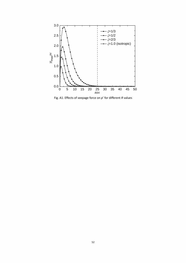
0 5 10 15 20 25 30 35 40 45 500.0
0.5
1.0
1.5
2.0
2.5
3.0
|I| m
ax/H
R/H
=1/3
=1/2
=2/3
=1.0 (isotropic)
Fig. A1. Effects of seepage force on p’ for different R values
53
List of Tables
Table 1 Comparison of proposed Pp values with Shield and Tolunay (1973)
Table 2 Comparison of proposed Kp values with other theoretical results
54
Table 1. Comparison of proposed Pp values with Shield and Tolunay (1973)
φ’(°) Proposed method Shield and Tolunay (1973)
Pp (kN) Ph(kN)* Pv(kN)* Pph(kN)** Pp
v(kN)** Pp (kN) Ph(kN) Pv(kN) Pph(kN) Pp
v(kN)
20 554.025 545.61 96.21 554.025 554.025 522.80 480.33 -206.43 390.25 -951.00
25 696.8 680.28 150.82 696.8 696.8 656.79 623.20 -207.35 510.75 -766.50
30 891.125 860.76 230.64 891.125 891.125 850.23 827.05 -197.20 685.00 -609.50
35 1192.05 1136.88 358.46 1192.05 1192.05 1142.28 1130.25 -165.38 948.00 -440.00
40 1650.5 1550.96 564.50 1650.5 1650.5 1607.55 1605.33 -84.63 1366.75 -209.75
45 2393.55 2211.35 915.97 2393.55 2393.55 2327.42 2326.03 80.70 2079.00 168.75 * Ph and Pv denote the horizontal and vertical component of the passive earth thrust Pp, respectively. ** Pp
h and Ppv denote the passive earth thrust obtained using the horizontal and vertical force equilibrium condition,
respectively.
55
Table 2. Comparison of proposed Kp values with other theoretical results
φ’ (°) δ/φ’ Proposed
method
Patki et al.
(2017)
Soubra
(2000)
Lancellotta
(2002)
Shiau
et al.
(2008)
Antão
et al.
(2011)
Patki et al.
(2015b)
20 1/3 2.09 2.39 2.39 2.37 2.42 2.39 2.86
1/2 2.22 2.57 2.58 2.52 2.62 2.56 3.01
2/3 2.39 2.75 2.77 2.65 2.82 2.73 3.17
1 2.55 3.13 3.12 2.87 3.21 3.05 3.51
25 1/3 2.54 3.07 3.08 3.03 3.11 3.07 3.64
1/2 2.79 3.41 3.43 3.30 3.48 3.39 3.95
2/3 3.11 3.76 3.79 3.56 3.86 3.72 4.26
1 3.43 4.54 4.51 4.00 4.70 4.36 5.03
30 1/3 3.16 4.03 4.05 3.95 4.10 4.02 4.72
1/2 3.56 4.65 4.69 4.44 4.76 4.62 5.31
2/3 4.19 5.34 5.40 4.93 5.49 5.25 5.94
1 4.98 6.93 6.86 5.80 7.14 6.56 7.59
35 1/3 4.06 5.44 5.48 5.28 5.58 5.42 6.27
1/2 4.77 6.59 6.67 6.16 6.77 6.52 7.38
2/3 5.53 7.95 8.06 7.09 8.17 7.76 8.64
1 8.10 11.31 11.13 8.85 11.50 10.58 12.23
40 1/3 5.39 7.62 7.70 7.28 7.79 7.57 8.62
1/2 6.60 9.81 9.99 8.92 10.03 9.67 10.75
2/3 8.44 12.58 12.93 10.71 12.87 12.19 13.30
1 13.00 20.01 19.62 14.39 20.10 18.15 21.49
45 1/3 7.41 11.18 11.36 10.48 11.41 11.09 12.38
1/2 9.57 15.61 15.98 13.60 15.85 15.29 16.59
2/3 13.22 21.78 22.22 17.27 22.03 20.75 22.09
1 23.50 39.91 38.61 25.47 45.14 34.99 42.40