1

Aquarius Workshop, Woods Hole, MA, USA11-12 May 2006

&

Observing regional salinity signals of major rivers: Exploring Aquarius and SMOS resolution limits

Derek Burrage, Joel Wesson, Jerry Miller, William Teague (NRL, USA), Carlos Martinez (UR, Uruguay) and Malcolm Heron (JCU,

Australia).

SMOS Workshop, Lyngby, Denmark15-18 May 2006

2

• Objectives and Motivation

• Airborne Observations

• Resolution Scales

• Land Correction

• Open Issues

Observing regional salinity signals of major rivers

3

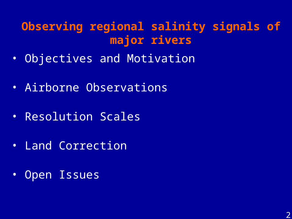
• Develop enhanced SSS products for the marginal seas and coastal transition zone.

• Validate enhanced SSS products by under-flying SMOS with NRL’s STARRS radiometer system.

• Assess and demonstrate benefits of enhanced products on coastal ocean data assimilation systems.

Objectives

SMOS Salinity Retrieval, Processing andPerformance in Coastal Regions and Marginal Seas

NRL ESA SMOS project AO-3229

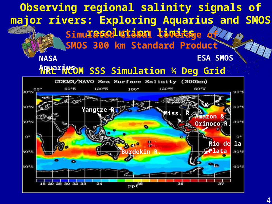
4

NRL NCOM SSS Simulation ¼ Deg Grid

Yangtze R.Miss. R. Amazon &

Orinoco R.

Rio de laPlataBurdekin R.

NASA Aquarius ESA SMOS

Observing regional salinity signals of major rivers: Exploring Aquarius and SMOS resolution limits

Simulated Global Coverage ofSMOS 300 km Standard Product

6

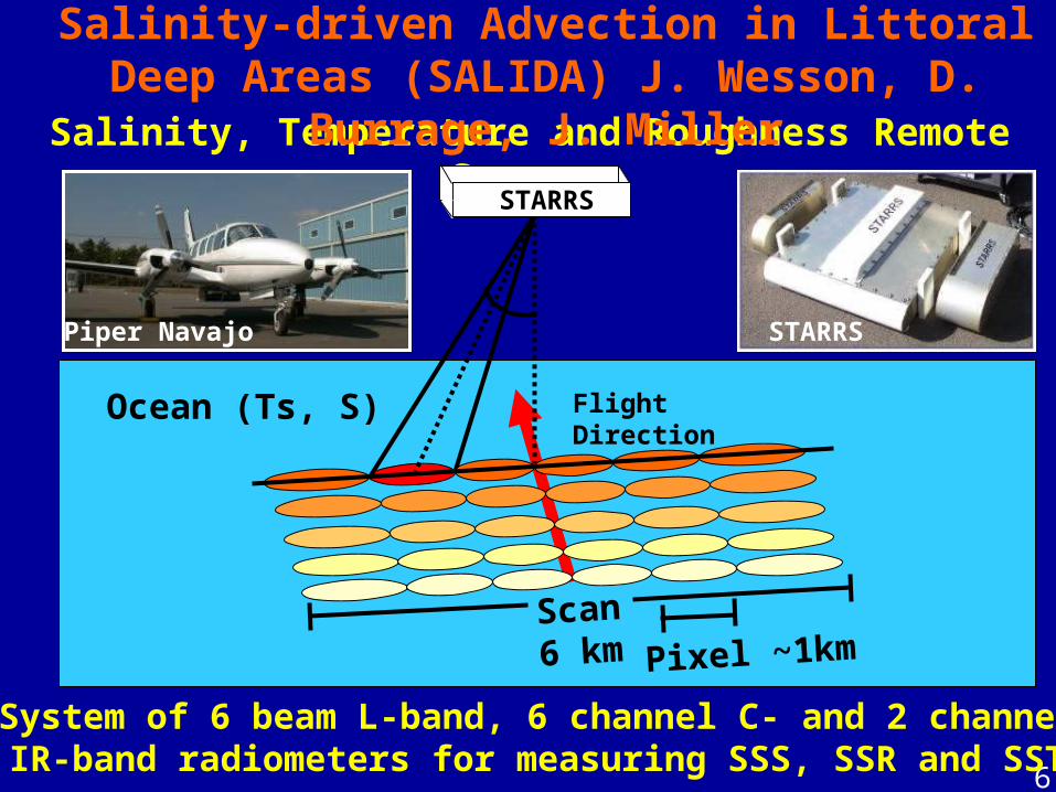
Scan6 km

FlightDirection

Ocean (Ts, S)

System of 6 beam L-band, 6 channel C- and 2 channelIR-band radiometers for measuring SSS, SSR and SST

Piper Navajo STARRS

Salinity, Temperature and Roughness Remote Scanner

Pixel ~1km

STARRS

Salinity-driven Advection in Littoral Deep Areas (SALIDA) J. Wesson, D. Burrage, J. Miller

7

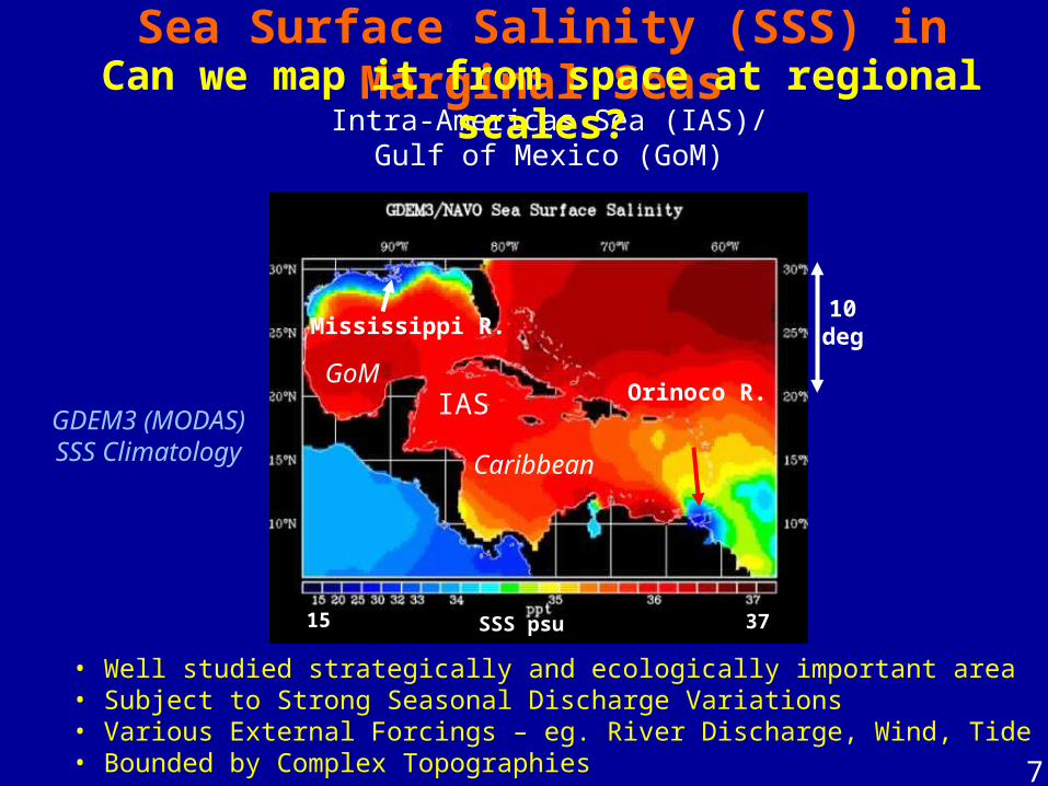
Sea Surface Salinity (SSS) in Marginal Seas

Intra-Americas Sea (IAS)/Gulf of Mexico (GoM)

GDEM3 (MODAS) SSS Climatology

Can we map it from space at regional scales?

IASGoM

15 SSS psu 37

Caribbean

10deg

• Well studied strategically and ecologically important area • Subject to Strong Seasonal Discharge Variations• Various External Forcings – eg. River Discharge, Wind, Tide• Bounded by Complex Topographies

Mississippi R.

Orinoco R.

8

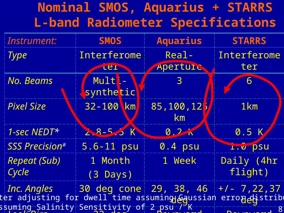
Nominal SMOS, Aquarius + STARRSL-band Radiometer Specifications

Instrument: SMOS Aquarius STARRS

Type Interferometer Real-Aperture Interferometer

No. Beams Multi-synthetic 3 6

Pixel Size 32-100 km 85,100,125 km 1km

1-sec NEDT* 2.8-5.5 K 0.2 K 0.5 K

SSS Precision# 5.6-11 psu 0.4 psu 1.0 psu

Repeat (Sub) Cycle

1 Month

(3 Days)

1 Week Daily (4hr flight)

Inc. Angles 30 deg cone 29, 38, 46 deg +/- 7,22,37 deg

Look Dirn 32 deg for’d tilt Downward Downward

Footprint 700 km Hex Transect 5 km Swath

*After adjusting for dwell time assuming Gaussian error distribution# Assuming Salinity Sensitivity of 2 psu / K

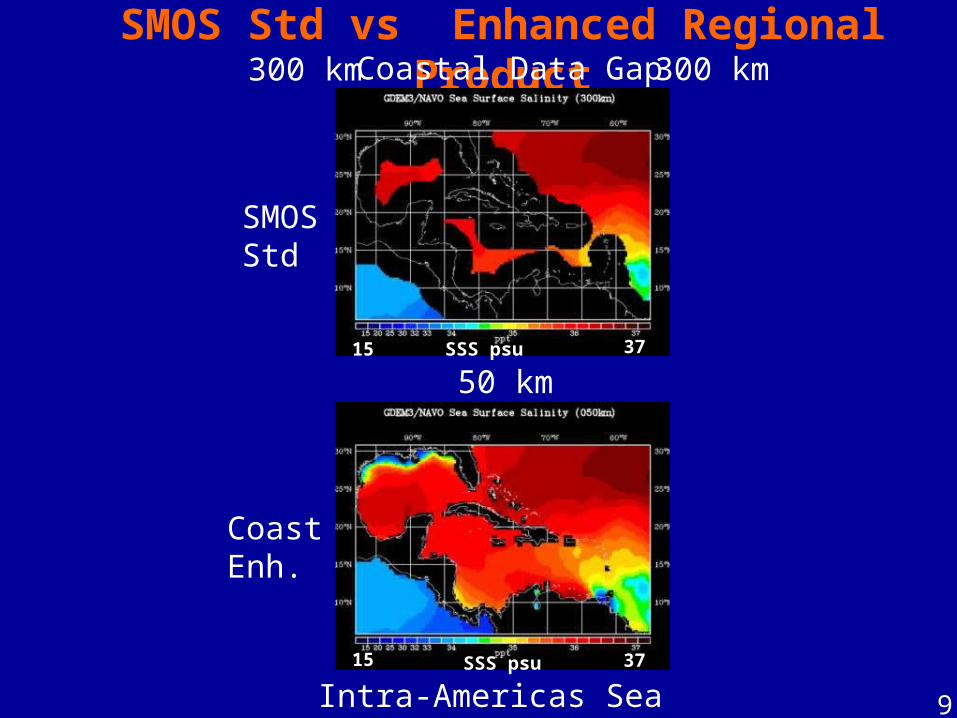
9

SMOS Std vs Enhanced Regional Product

SMOSStd

Coastal Data Gap

50 km

CoastEnh.

Intra-Americas Sea15 37SSS psu

SSS psu 3715

300 km300 km

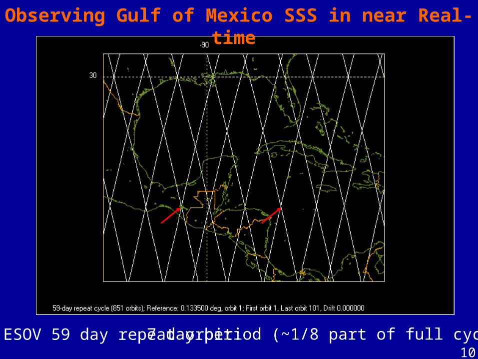
107 day period (~1/8 part of full cycle)

Observing Gulf of Mexico SSS in near Real-time

ESOV 59 day repeat orbit:

112 day period (wide swath => full coverage) ESOV 59 day repeat orbit:

GoM SMOS Coverage – Wide Swath

12

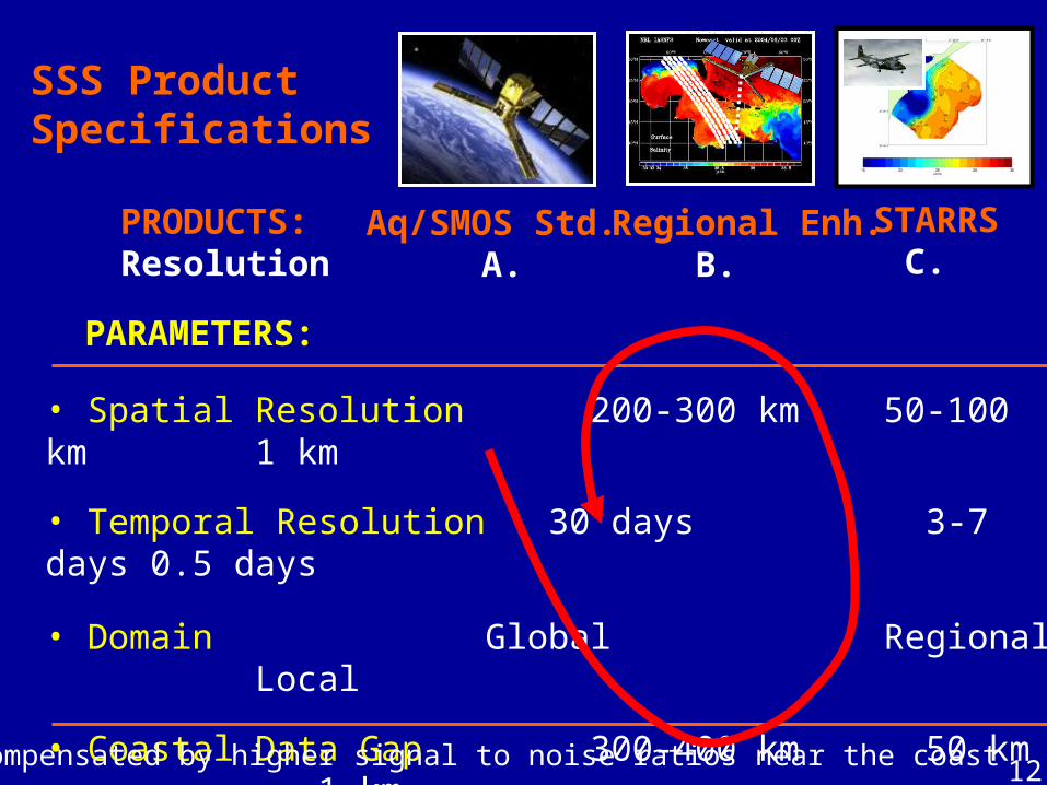
• Spatial Resolution 200-300 km 50-100 km 1 km

• Temporal Resolution 30 days 3-7 days 0.5 days

• Domain Global Regional Local

• Coastal Data Gap 300-400 km 50 km 1 km

• Salinity Error (psu) 0.1 0.5-2.0* 1.0

PARAMETERS:

Aq/SMOS Std. A.

Regional Enh.B.

PRODUCTS:Resolution

STARRSC.

* Compensated by higher signal to noise ratios near the coast

SSS ProductSpecifications

13

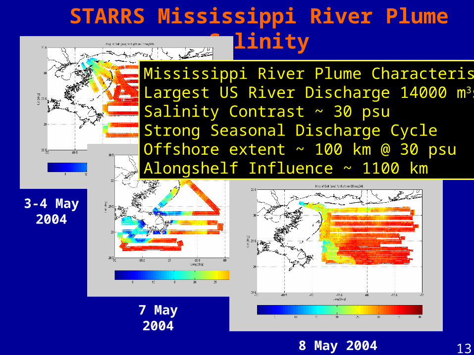
STARRS Mississippi River Plume Salinity

7 May2004

8 May 2004

3-4 May2004

Mississippi River Plume CharacteristicsLargest US River Discharge 14000 m3s-1

Salinity Contrast ~ 30 psuStrong Seasonal Discharge CycleOffshore extent ~ 100 km @ 30 psuAlongshelf Influence ~ 1100 km

14

230 240 250 260 270 280 290 300 310 32080

85

90

95

100

105

110

115

120

125

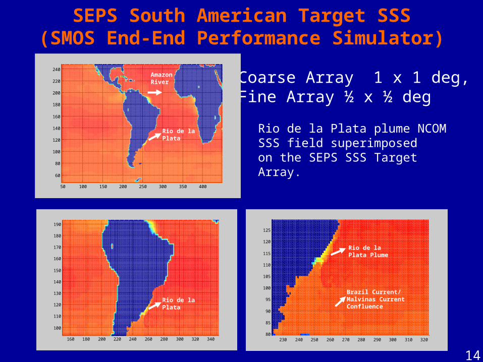
SEPS South American Target SSS(SMOS End-End Performance Simulator)

Coarse Array 1 x 1 deg,Fine Array ½ x ½ deg

50 100 150 200 250 300 350 400

60

80

100

120

140

160

180

200

220

240

160 180 200 220 240 260 280 300 320 340

100

110

120

130

140

150

160

170

180

190

Rio de laPlata

Rio de laPlata Plume

Rio de laPlata

AmazonRiver

Brazil Current/Malvinas CurrentConfluence

Rio de la Plata plume NCOMSSS field superimposedon the SEPS SSS TargetArray.

15

50 100 150 200 250 300 350 400

60

80

100

120

140

160

180

200

220

240

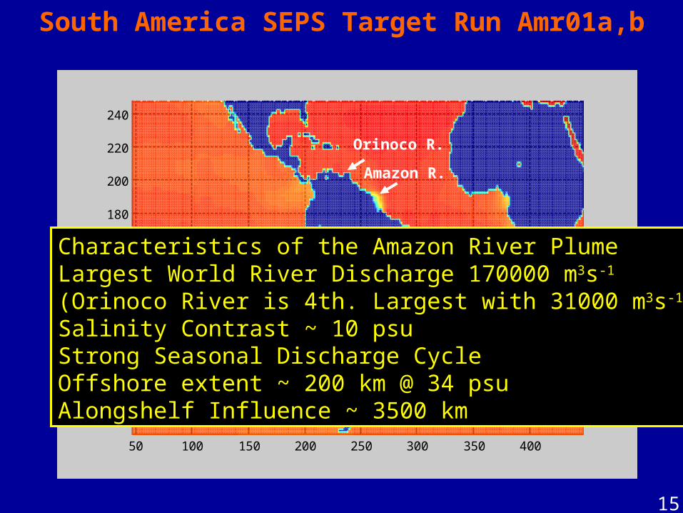
South America SEPS Target Run Amr01a,b

Characteristics of the Amazon River PlumeLargest World River Discharge 170000 m3s-1

(Orinoco River is 4th. Largest with 31000 m3s-1)Salinity Contrast ~ 10 psuStrong Seasonal Discharge CycleOffshore extent ~ 200 km @ 34 psuAlongshelf Influence ~ 3500 km

Amazon R.

Orinoco R.

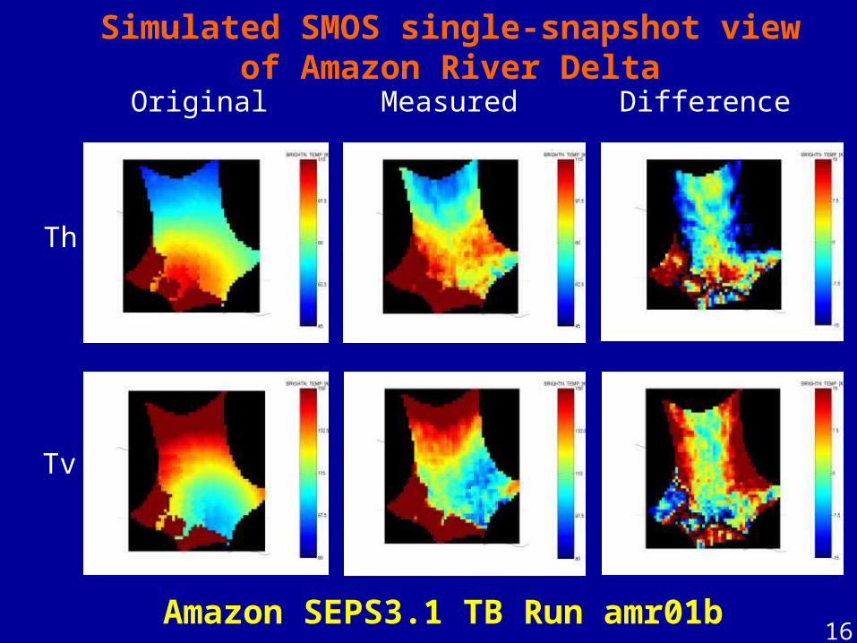
16Amazon SEPS3.1 TB Run amr01b

Original DifferenceMeasured

Th

Tv

Simulated SMOS single-snapshot viewof Amazon River Delta

17

50 100 150 200 250 300 350 400

60

80

100

120

140

160

180

200

220

240

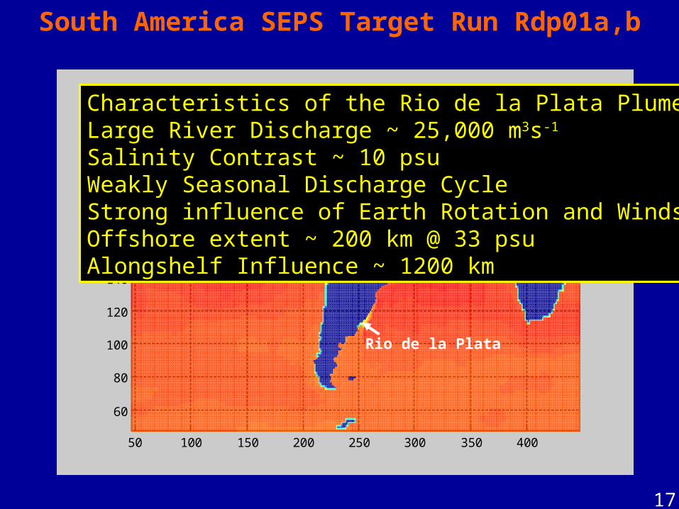
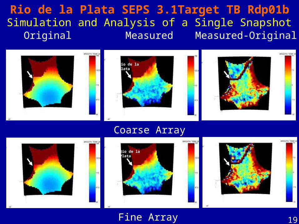
South America SEPS Target Run Rdp01a,b

Characteristics of the Rio de la Plata PlumeLarge River Discharge ~ 25,000 m3s-1

Salinity Contrast ~ 10 psuWeakly Seasonal Discharge CycleStrong influence of Earth Rotation and WindsOffshore extent ~ 200 km @ 33 psuAlongshelf Influence ~ 1200 km

Rio de la Plata

18

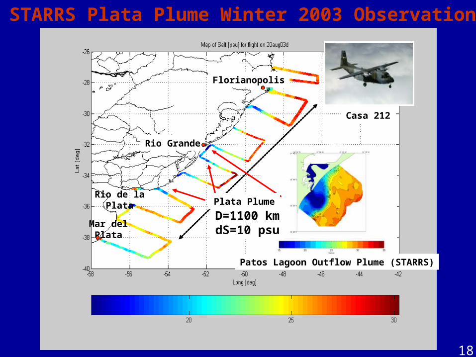
STARRS Plata Plume Winter 2003 Observations

Mar del Plata

Florianopolis

Patos Lagoon Outflow Plume (STARRS)

Rio Grande

Plata Plume

D=1100 kmdS=10 psu

Rio de laPlata

Casa 212

19

Rio de la Plata SEPS 3.1Target TB Rdp01bSimulation and Analysis of a Single Snapshot

Fine Array

Coarse Array

Original Measured Measured-Original

Rio de laPlata

Rio de laPlata

20

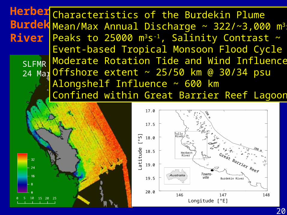
Herbert-BurdekinRiver System

SLFMR SSS Map24 Mar., 2000

2520151050146 147 148

20.0

19.5

19.0

18.5

18.0

17.5

17.0 200 m

200 m

Tully River

Herbert River

Burdekin River

Towns- ville

Great Barrier Reef

La

titu

de

[°S

]

Longitude [°E]

Characteristics of the Burdekin PlumeMean/Max Annual Discharge ~ 322/~3,000 m3s-1

Peaks to 25000 m3s-1, Salinity Contrast ~ 10 psuEvent-based Tropical Monsoon Flood CycleModerate Rotation Tide and Wind InfluenceOffshore extent ~ 25/50 km @ 30/34 psuAlongshelf Influence ~ 600 kmConfined within Great Barrier Reef Lagoon

21

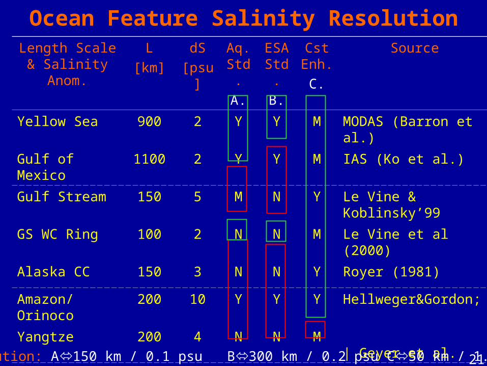
Length Scale & Salinity Anom.

L

[km]

dS

[psu]

Aq. Std.

A.

ESAStd.

B.

Cst Enh.

C.

Source

Yellow Sea 900 2 Y Y M MODAS (Barron et al.)

Gulf of Mexico 1100 2 Y Y M IAS (Ko et al.)

Gulf Stream 150 5 M N Y Le Vine & Koblinsky’99

GS WC Ring 100 2 N N M Le Vine et al (2000)

Alaska CC 150 3 N N Y Royer (1981)

Amazon/Orinoco

200 10 Y Y Y Hellweger&Gordon;

Yangtze 200 4 N N M | Geyer et al.

Plata Plume 200 10 N N Y Martinez et al (2005)

Miss.Plume 100 30 N N Y STARRS Burrage et al

Burdekin Plume 50 10 N N N SLFMR Burrage/Heron

Resolution: A150 km / 0.1 psu B300 km / 0.2 psu C50 km / 1.0 psu

Ocean Feature Salinity Resolution

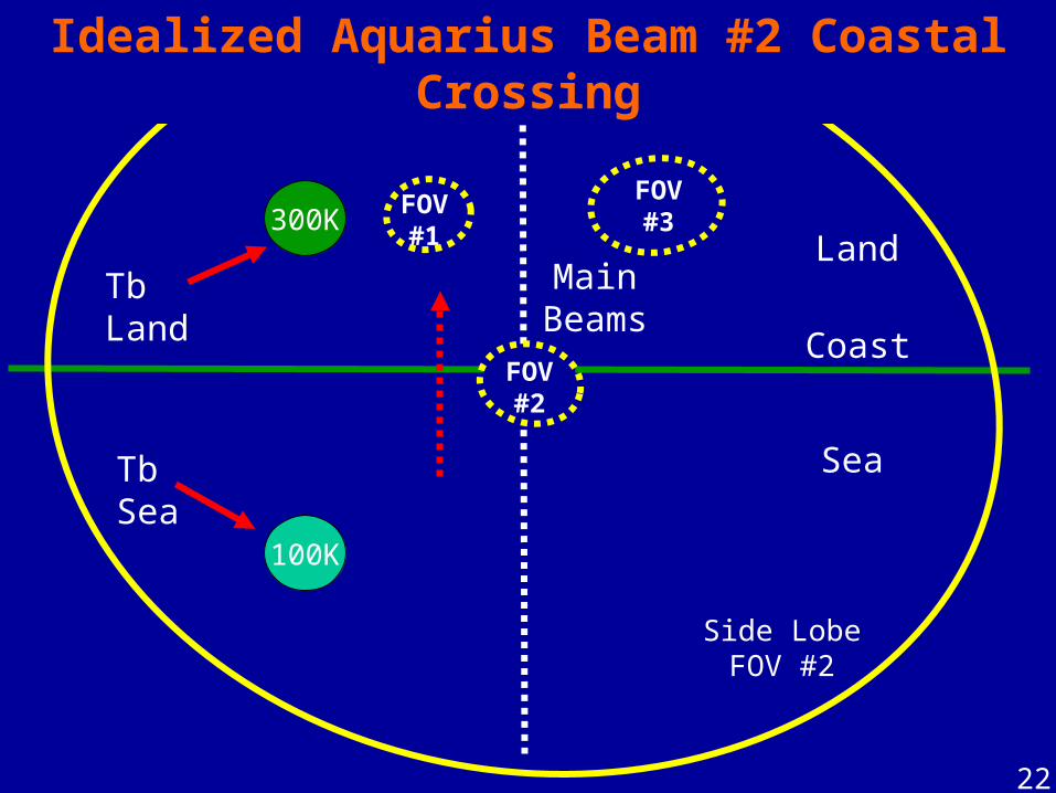
22

LandMain

Beams

Idealized Aquarius Beam #2 Coastal Crossing

Side LobeFOV #2

SeaTbSea

TbLand

300KFOV #1

FOV #3

FOV #2

100K

Coast

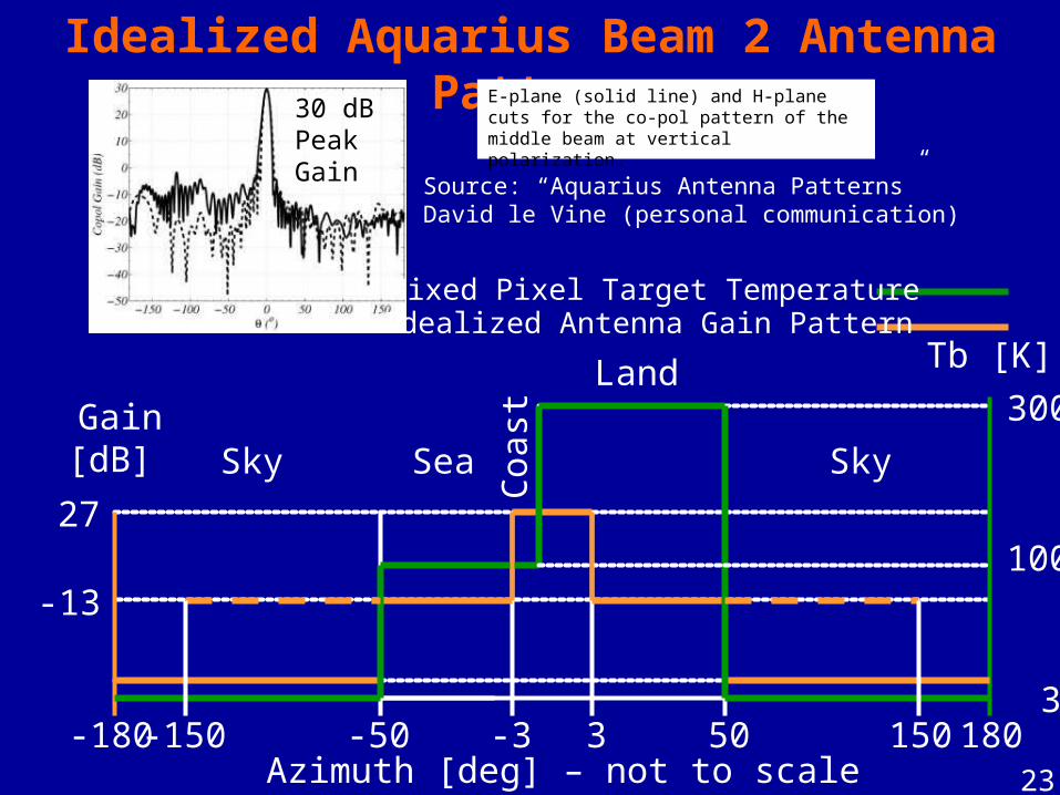
23

Idealized Aquarius Beam 2 Antenna PatternE-plane (solid line) and H-plane cuts for the co-pol pattern of the middle beam at vertical polarization.

Source: “Aquarius Antenna Patterns”David le Vine (personal communication)

30 dBPeakGain

Mixed Pixel Target TemperatureIdealized Antenna Gain Pattern

Tb [K]

-50 -180 180 -3 3 50

27

Gain[dB]

Azimuth [deg] – not to scale

-13

Sky

Land

Sea Sky

3

100

300

Coa

st

150 -150

24

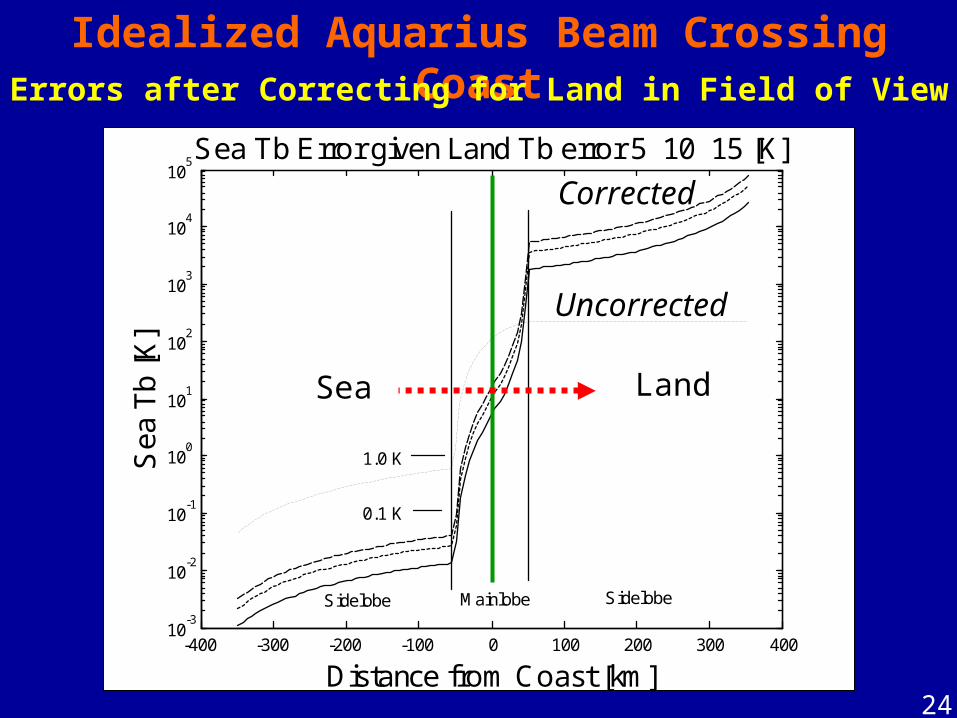
Idealized Aquarius Beam Crossing Coast

-400 -300 -200 -100 0 100 200 300 40010

-3

10-2

10-1

100

101

102

103

104

105

Distance from Coast [km]

Sea

Tb

[K]

Sea Tb Error given Land Tb error 5 10 15 [K]

Mainlobe Sidelobe Sidelobe

1.0 K

0.1 K

Errors after Correcting for Land in Field of View

Sea Land

Uncorrected

Corrected

25

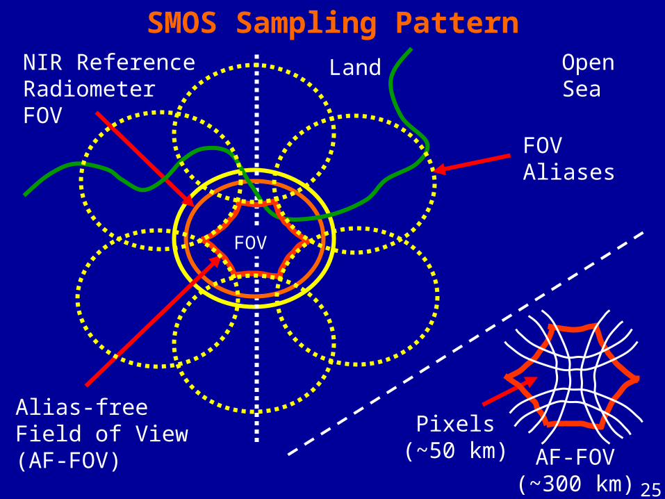
SMOS Sampling PatternNIR ReferenceRadiometerFOV

FOV

OpenSea

Land

Pixels(~50 km) AF-FOV

(~300 km)

Alias-freeField of View(AF-FOV)

FOVAliases

26

STARRS Mixed-Pixel SurveyNIR ReferenceRadiometerFOV

Sea

Land

Alias-freeField of View(AF-FOV)

Coast

MIRASPixels

MixedPixel

STARRSFlightLines ~50

km

27

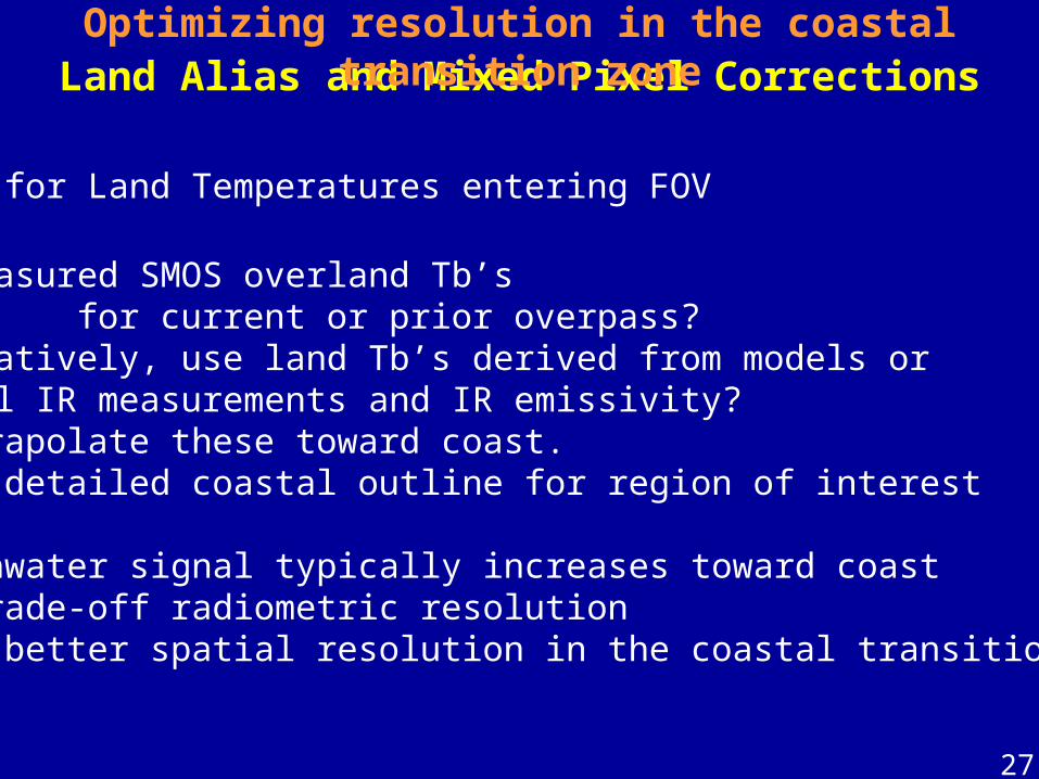
• Account for Land Temperatures entering FOV

Use measured SMOS overland Tb’s for current or prior overpass?

Alternatively, use land Tb’s derived from models orThermal IR measurements and IR emissivity?

Extrapolate these toward coast.Use detailed coastal outline for region of interest

• SSS Freshwater signal typically increases toward coast=> Can trade-off radiometric resolution

for better spatial resolution in the coastal transition zone

Land Alias and Mixed Pixel CorrectionsOptimizing resolution in the coastal transition zone

28

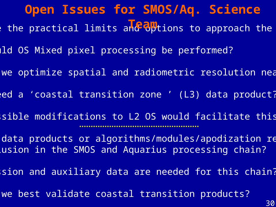
What are the practical limits and options to approach the coast?

How should OS Mixed pixel processing be performed?

How can we optimize spatial and radiometric resolution near coasts?

Do we need a ‘coastal transition zone ’ (L3) data product?

What possible modifications to L2 OS would facilitate this?

Are new data products or algorithms/modules/apodization requiredfor inclusion in the SMOS and Aquarius processing chain?

What mission and auxiliary data are needed for this chain?

How can we best validate coastal transition products?

Open Issues for SMOS/Aq. Science Team

29

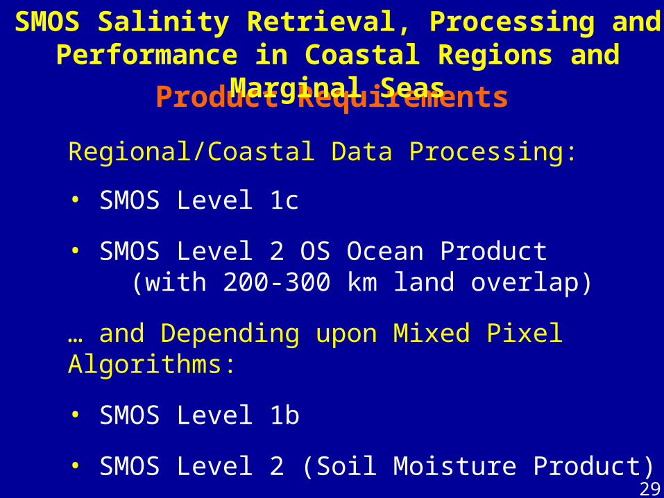
Regional/Coastal Data Processing:

• SMOS Level 1c

• SMOS Level 2 OS Ocean Product (with 200-300 km land overlap)

… and Depending upon Mixed Pixel Algorithms:

• SMOS Level 1b

• SMOS Level 2 (Soil Moisture Product)

Product Requirements

SMOS Salinity Retrieval, Processing and Performance in Coastal Regions and Marginal Seas

30

What are the practical limits and options to approach the coast?

How should OS Mixed pixel processing be performed?

How can we optimize spatial and radiometric resolution near coasts?

Do we need a ‘coastal transition zone ’ (L3) data product?

What possible modifications to L2 OS would facilitate this?

Are new data products or algorithms/modules/apodization requiredfor inclusion in the SMOS and Aquarius processing chain?

What mission and auxiliary data are needed for this chain?

How can we best validate coastal transition products?

Open Issues for SMOS/Aq. Science Team