1. Basis pursuit denoise. Ax b m n - Optimization Online · 1 subject to kAx bk 2 ˙; where the positive parameter ˙is an estimate of the noise level in the data. The case ˙= 0

Department of Computer Science, University of British ColumbiaTechnical Report TR-2008-01, January 2008 (revised May 2008)

PROBING THE PARETO FRONTIER FORBASIS PURSUIT SOLUTIONS

EWOUT VAN DEN BERG AND MICHAEL P. FRIEDLANDER∗

Abstract. The basis pursuit problem seeks a minimum one-norm solution of an underdeterminedleast-squares problem. Basis pursuit denoise (BPDN) fits the least-squares problem only approximately,and a single parameter determines a curve that traces the optimal trade-off between the least-squaresfit and the one-norm of the solution. We prove that this curve is convex and continuously differentiableover all points of interest, and show that it gives an explicit relationship to two other optimizationproblems closely related to BPDN.

We describe a root-finding algorithm for finding arbitrary points on this curve; the algorithmis suitable for problems that are large scale and for those that are in the complex domain. At eachiteration, a spectral gradient-projection method approximately minimizes a least-squares problemwith an explicit one-norm constraint. Only matrix-vector operations are required. The primal-dualsolution of this problem gives function and derivative information needed for the root-finding method.Numerical experiments on a comprehensive set of test problems demonstrate that the method scaleswell to large problems.

Key words. basis pursuit, convex program, duality, root-finding, Newton’s method, projectedgradient, one-norm regularization, sparse solutions

AMS subject classifications. 49M29, 65K05, 90C25, 90C06

1. Basis pursuit denoise. The basis pursuit problem aims to find a sparsesolution of the underdetermined system of equations Ax = b, where A is an m-by-nmatrix and b is an m-vector. Typically, m � n, and the problem is ill-posed. Theapproach advocated by Chen et al. [15] is to solve the convex optimization problem

(BP) minimizex

‖x‖1 subject to Ax = b.

In the presence of noisy or imperfect data, however, it is undesirable to exactly fit thelinear system. Instead, the constraint in (BP) is relaxed to obtain the basis pursuitdenoise (BPDN) problem

(BPσ) minimizex

‖x‖1 subject to ‖Ax− b‖2 ≤ σ,

where the positive parameter σ is an estimate of the noise level in the data. The caseσ = 0 corresponds to a solution of (BP)—i.e., a basis pursuit solution.

There is now a significant body of work that addresses the conditions underwhich a solution of this problem yields a sparse approximation to a solution of theunderdetermined system; see Candes, Romberg, and Tao [11], Donoho [24], andTropp [48], and references therein. The sparse approximation problem is of vitalimportance to many applications in signal processing and statistics. Some importantapplications include image reconstruction, such as MRI [36, 37] and seismic [31, 32]images, and model selection in regression [26]. In many of these applications, thedata sets are large, and the matrix A is available only as an operator. In compressedsensing [10–12,23], for example, the matrices are often fast operators such as Fourieror wavelet transforms. It is therefore crucial to develop algorithms for the sparsereconstruction problem that scale well and work effectively in a matrix-free context.

∗Department of Computer Science, University of British Columbia, Vancouver V6T 1Z4, B.C.,Canada ({ewout78,mpf}@cs.ubc.ca). Friedlander is corresponding author. This work was supportedby the NSERC Collaborative Research and Development Grant 334810-05. May 30, 2008

1

2 E. van den BERG and M. P. FRIEDLANDER

We present an algorithm, suitable for large-scale applications, that is capable offinding solutions of (BPσ) for any value of σ ≥ 0. Our approach is based on recasting(BPσ) as a problem of finding the root of a single-variable nonlinear equation. Ateach iteration of our algorithm, an estimate of that variable is used to define a convexoptimization problem whose solution yields derivative information that can be usedby a Newton-based root finding algorithm.

1.1. One-norm regularization. The convex optimization problem (BPσ) isonly one possible statement of the one-norm regularized least-squares problem. Infact, the BPDN label is typically applied to the penalized least-squares problem

(QPλ) minimizex

‖Ax− b‖22 + λ‖x‖1,

which is the problem statement proposed by Chen et al. [14, 15]. A third formulation,

(LSτ ) minimizex

‖Ax− b‖2 subject to ‖x‖1 ≤ τ,

has an explicit one-norm constraint and is often called the Lasso problem [46]. Theparameter λ is related to the Lagrange multiplier of the constraint in (LSτ ) and to thereciprocal of the multiplier of the constraint in (BPσ). Thus, for appropriate parameterchoices of σ, λ, and τ , the solutions of (BPσ), (QPλ), and (LSτ ) coincide, and theseproblems are in some sense equivalent. However, except for special cases—such as Aorthogonal—the parameters that make these problems equivalent cannot be known apriori.

The formulation (QPλ) is often preferred because of its close connection to convexquadratic programming, for which many algorithms and software are available; someexamples include iteratively reweighted least squares [7, section 4.5] and gradientprojection [27]. For the case where an estimate of the noise-level σ is known, Chenet al. [15, section 5.2] argue that the choice λ = σ

√2 log n has important optimality

properties. However, this argument hinges on the orthogonality of A.We focus on the situation where σ is approximately known—such as when we can

estimate the noise levels inherent in an underlying system or in the measurementstaken. In this case it is preferable to solve (BPσ), and here this is our primary goal. Animportant consequence of our approach is that it can also be used to efficiently solvethe closely related problems (BP) and (LSτ ). Our algorithm also applies to all threeproblems in the complex domain, which can arise in signal processing applications.

1.2. Approach. At the heart of our approach is the ability to efficiently solve asequence of (LSτ ) problems using a spectral projected-gradient (SPG) algorithm [5,6,18].As with (QPλ), this problem is parameterized by a scalar; the crucial difference, however,is that the dual solution of (LSτ ) yields vital information on how to update τ so thatthe next solution of (LSτ ) is much closer to the solution of (BPσ).

Let xτ denote the optimal solution of (LSτ ). The single-parameter function

φ(τ) = ‖rτ‖2 with rτ := b−Axτ (1.1)

gives the optimal value of (LSτ ) for each τ ≥ 0. As we describe in section 2, its derivativeis given by −λτ , where λτ ≥ 0 is the unique dual solution of (LSτ ). Importantly, thisdual solution can easily be obtained as a by-product of the minimization of (LSτ ); this

PROBING THE PARETO FRONTIER FOR BASIS PURSUIT SOLUTIONS 3

is discussed in section 2.1. Our approach is then based on applying Newton’s methodto find a root of the nonlinear equation

φ(τ) = σ, (1.2)

which defines a sequence of regularization parameters τk → τσ, where xτσ is a solutionof (BPσ). In other words, τσ is the parameter that causes (LSτ ) and (BPσ) to sharethe same solution.

There are four distinct components to this paper. The first two are related tothe root-finding algorithm for (BPσ). The third is an efficient algorithm for solving(LSτ )—and hence for evaluating the function φ and its derivative φ′. The fourth givesthe results of a series of numerical experiments.

Pareto curve (section 2). The Pareto curve defines the optimal trade-off betweenthe two-norm of the residual r and the one-norm of the solution x. The problems(BPσ) and (LSτ ) are two distinct characterizations of the same curve. Our approachuses the function φ to parameterize the Pareto curve by τ . We show that for all pointsof interest, φ—and hence the Pareto curve—is continuously differentiable. We are alsoable to give an explicit expression for its derivative. This surprising result permits usto use a Newton-based root-finding algorithm to find roots of the nonlinear equation(1.2), which correspond to points on the Pareto curve. Thus we can find solutions of(BPσ) for any σ ≥ 0.

Root finding (section 3). Each iteration of the root-finding algorithm for (1.2)requires the evaluation of φ and φ′ at some τ , and hence the minimization of (LSτ ).This is a potentially expensive subproblem, and the effectiveness of our approachhinges on the ability to solve this subproblem only approximately. We present rate-of-convergence results for the case where φ and φ′ are known only approximately. This isin contrast to the usual inexact-Newton analysis [22], which assumes that φ is knownexactly. We also give an effective stopping rule for determining the required accuracyof each minimization of (LSτ ).

Projected gradient for Lasso (section 4). We describe an SPG algorithm for solving(LSτ ). Each iteration of this method requires an orthogonal projection of an n-vectoronto the convex set ‖x‖1 ≤ τ . In section 4.2 we give an algorithm for this projectionwith a worst-case complexity of O(n log n). In many important applications, A is aFourier-type operator, and matrix-vector products with A and AT can be obtainedwith O(n log n) cost. The projection cost is typically much smaller than the worst-case,and the dominant cost in our algorithm consists of the matrix-vector products, as itdoes in other algorithms for basis pursuit denoise. We also show how the projectionalgorithm can easily be extended to project complex vectors, which allows us to extendthe SPG algorithm to problems in the complex domain.

Implementation and numerical experiments (sections 5 and 6). To demonstrate theeffectiveness of our approach, we run our algorithm on a set of benchmark problems andcompare it to other state-of-the-art solvers. In sections 6.1 and 6.2 we report numericalresults on a series of (BPσ) and (BP) problems, which are normally considered as distinctproblems. In section 6.3 we report numerical results on a series of (LSτ ) problemsfor various values of τ , and compare against the equivalent (QPλ) formulations. Insection 6.4 we show how to capitalize on the smoothness of the Pareto curve to obtainquick and approximate solutions to (BPσ).

1.3. Assumption. We make the following blanket assumption throughout:Assumption 1.1. The vector b ∈ range(A), and b 6= 0. This assumption is only

needed in order to simplify the discussion, and it implies that (BPσ) is feasible for all


σ ≥ 0. In many applications, such as compressed sensing [10–12,23], A has full rowrank, and therefore this assumption is satisfied automatically.

1.4. Related work.Homotopy approaches. A number of approaches have been suggested for solving

(BPσ), many of which are based on repeatedly solving (QPλ) for various values of λ.Notable examples of this approach are Homotopy [41, 42] and Lars [26], which solve(QPλ) for essentially all values of λ. In this way, they eventually find the value of λthat recovers a solution of (BPσ). These active-set continuation approaches begin withλ = ‖AT b‖∞ (for which the corresponding solution is xλ = 0), and gradually reduce λin stages that predictably change the sparsity pattern in xλ. The remarkable efficiencyof these continuation methods follows from their ability to systematically update theresulting sequence of solutions. (See Donoho and Tsaig [25] and Friedlander andSaunders [28] for discussions of the performance of these methods.) The computationalbottleneck for these methods is the accurate solution at each iteration of a least-squaressubproblem that involves a subset of the columns of A. In some applications (such asthe seismic image reconstruction problem [32]) the size of this subset can become large,and thus the least-squares subproblems can become prohibitively expensive. Moreover,even if the correct value λσ is known a priori, the method must necessarily begin withλ = ‖AT b‖∞ and traverse all critical values of λ down to λσ.

Basis pursuit denoise as a cone program. The problem (BPσ) with σ > 0 canbe considered as a special case of a generic second-order cone program [8, Ch. 5].Interior-point (IP) algorithms for general conic programs can be very effective ifthe matrices are available explicitly. Examples of general-purpose software for coneprograms include SeDuMi [45] and MOSEK [39]. The software package `1-magic [9]contains an IP implementation specially adapted to (BPσ). In general, the efficiency ofIP implementations relies ultimately on their ability to efficiently solve certain linearsystems that involve highly ill-conditioned matrices.

Basis pursuit as a linear program. The special case σ = 0 corresponding to (BP)can be reformulated and solved as a linear program. Again, IP methods are knownto be effective for general linear programs, but many IP implementations for generallinear programming, such as CPLEX [16] and MOSEK, require explicit matrices. Thesolver PDCO [44], available within the SparseLab package, is capable of using A as anoperator only, but it often requires many matrix-vector multiplications to converge,and as we report in section 6.2, it is not generally competitive with other approaches.We are not aware of simplex-type implementations that do not require A explicitly.

Sampling the Pareto curve. A common approach for obtaining approximate solu-tions to (BPσ) is to sample various points on the Pareto curve; this is often accomplishedby solving (QPλ) for a decreasing sequence of values of λ. As noted by Das and Den-nis [19], and more recently by Leyffer [35], a uniform distribution of weights λ can leadto an uneven sampling of the Pareto curve. In contrast, by instead parameterizing thePareto curve by σ or τ (via the problem (BPσ) or (LSτ )), it is possible to obtain amore uniform sample of the Pareto curve; see section 6.4.

Projected gradient. Our application of the SPG algorithm to solve (LSτ ) followsBirgin et al. [5] closely for minimization of general nonlinear functions over arbitraryconvex sets. The method they propose combines projected-gradient search directionswith the spectral step length that was introduced by Barzilai and Borwein [1]. Anonmonotone linesearch is used to accept or reject steps. The key ingredient of Birginet al.’s algorithm is the projection of the gradient direction onto a convex set, whichin our case is defined by the constraint in (LSτ ). In their recent report, Figueiredo


0 1 2 3 4 5 6 70

5

10

15

20

25

one−norm of solution

two−

norm

of r

esid

ual

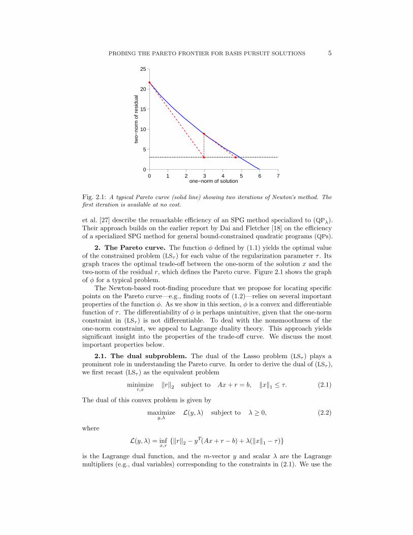
Fig. 2.1: A typical Pareto curve (solid line) showing two iterations of Newton’s method. Thefirst iteration is available at no cost.

et al. [27] describe the remarkable efficiency of an SPG method specialized to (QPλ).Their approach builds on the earlier report by Dai and Fletcher [18] on the efficiencyof a specialized SPG method for general bound-constrained quadratic programs (QPs).

2. The Pareto curve. The function φ defined by (1.1) yields the optimal valueof the constrained problem (LSτ ) for each value of the regularization parameter τ . Itsgraph traces the optimal trade-off between the one-norm of the solution x and thetwo-norm of the residual r, which defines the Pareto curve. Figure 2.1 shows the graphof φ for a typical problem.

The Newton-based root-finding procedure that we propose for locating specificpoints on the Pareto curve—e.g., finding roots of (1.2)—relies on several importantproperties of the function φ. As we show in this section, φ is a convex and differentiablefunction of τ . The differentiability of φ is perhaps unintuitive, given that the one-normconstraint in (LSτ ) is not differentiable. To deal with the nonsmoothness of theone-norm constraint, we appeal to Lagrange duality theory. This approach yieldssignificant insight into the properties of the trade-off curve. We discuss the mostimportant properties below.

2.1. The dual subproblem. The dual of the Lasso problem (LSτ ) plays aprominent role in understanding the Pareto curve. In order to derive the dual of (LSτ ),we first recast (LSτ ) as the equivalent problem

minimizer,x

‖r‖2 subject to Ax+ r = b, ‖x‖1 ≤ τ. (2.1)

The dual of this convex problem is given by

maximizey,λ

L(y, λ) subject to λ ≥ 0, (2.2)

where

L(y, λ) = infx,r{‖r‖2 − yT(Ax+ r − b) + λ(‖x‖1 − τ)}

is the Lagrange dual function, and the m-vector y and scalar λ are the Lagrangemultipliers (e.g., dual variables) corresponding to the constraints in (2.1). We use the


separability of the infimum in r and x to rearrange terms and arrive at the equivalentstatement

L(y, λ) = bTy − τλ− supr{yTr − ‖r‖2} − sup

x{yTAx− λ‖x‖1}.

We recognize the suprema above as the conjugate functions of ‖r‖2 and of λ‖x‖1,respectively. For an arbitrary norm ‖ · ‖ with dual norm ‖ · ‖∗, the conjugate functionof f(x) = α‖x‖ for any α ≥ 0 is given by

f∗(y) := supx{yTx− α‖x‖} =

{0 if ‖y‖∗ ≤ α,∞ otherwise;

(2.3)

see Boyd and Vandenberghe [8, section 3.3.1]. With this expression of the conjugatefunction, it follows that (2.2) remains bounded if and only if the dual variables y andλ satisfy the constraints ‖y‖2 ≤ 1 and ‖ATy‖∞ ≤ λ. The dual of (2.1), and hence of(LSτ ), is then given by

maximizey,λ

bTy − τλ subject to ‖y‖2 ≤ 1, ‖ATy‖∞ ≤ λ; (2.4)

the nonnegativity constraint on λ is implicitly enforced by the second constraint.Importantly, the dual variables y and λ can easily be computed from the optimal

primal solutions. To derive y, first note that from (2.3),

supr{yTr − ‖r‖2} = 0 if ‖y‖2 ≤ 1. (2.5)

Therefore, y = r/‖r‖2, and we can without loss of generality take ‖y‖2 = 1 in (2.4).To derive λ, note that as long as τ > 0, λ must be at its lower bound, as implied bythe constraint ‖ATy‖∞ ≤ λ. Hence, we take λ = ‖ATy‖∞. (If r = 0 or τ = 0, thechoice of y or λ, respectively, is arbitrary.) The dual variable y can then be eliminated,and we arrive at the following necessary and sufficient optimality conditions for theprimal-dual solution (rτ , xτ , λτ ) of (2.1):

Axτ + rτ = b, ‖xτ‖1 ≤ τ (primal feasibility); (2.6a)

‖ATrτ‖∞ ≤ λτ‖rτ‖2 (dual feasibility); (2.6b)λτ (‖xτ‖1 − τ) = 0 (complementarity). (2.6c)

2.2. Convexity and differentiability of the Pareto curve. Let τBP be theoptimal objective value of the problem (BP). This corresponds to the smallest valueof τ such that (LSτ ) has a zero objective value. As we show below, φ is nonincreasing,and therefore τBP is the first point at which the graph of φ touches the horizontal axis.Our assumption that 0 6= b ∈ range(A) implies that (BP) is feasible, and that τBP > 0.Therefore, at the endpoints of the interval of interest,

φ(0) = ‖b‖2 > 0 and φ(τBP) = 0. (2.7)

As the following result confirms, the function is convex and strictly decreasing overthe interval τ ∈ [0, τBP]. It is also continuously differentiable on the interior of thisinterval—this is a crucial property.


Theorem 2.1.(a) The function φ is convex and nonincreasing.(b) For all τ ∈ (0, τBP), φ is continuously differentiable, φ′(τ) = −λτ , and the

optimal dual variable λτ = ‖ATyτ‖∞, where yτ = rτ/‖rτ‖2.(c) For τ ∈ [0, τBP], ‖xτ‖1 = τ , and φ is strictly decreasing.

Proof. (a) The function φ can be restated as

φ(τ) = infxf(x, τ), (2.8)

where

f(x, τ) := ‖Ax− b‖2 + ψτ (x) and ψτ (x) :=

{0 if ‖x‖1 ≤ τ ,∞ otherwise.

Note that by (2.3), ψτ (x) = supz{xTz − τ‖z‖∞}, which is the pointwise supremumof an affine function in (x, τ). Therefore it is convex in (x, τ). Together with theconvexity of ‖Ax−b‖2, this implies that f is convex in (x, τ). Consider any nonnegativescalars τ1 and τ2, and let x1 and x2 be the corresponding minimizers of (2.8). For anyβ ∈ [0, 1],

φ(βτ1 + (1− β)τ2) = infxf(x, βτ1 + (1− β)τ2)

≤ f(βx1 + (1− β)x2 , βτ1 + (1− β)τ2

)≤ βf(x1, τ1) + (1− β)f(x2, τ2)= βφ(τ1) + (1− β)φ(τ2).

Hence, φ is convex in τ . Moreover, φ is nonincreasing because the feasible set enlargesas τ increases.

(b) The function φ is differentiable at τ if and only if its subgradient at τ is unique[43, Theorem 25.1]. By [4, Proposition 6.5.8(a)], −λτ ∈ ∂φ(τ). Therefore, to provedifferentiability of φ it is enough show that λτ is unique. Note that λ appears linearlyin (2.4) with coefficient −τ < 0, and thus λτ is not optimal unless it is at its lowerbound, as implied by the constraint ‖ATy‖∞ ≤ λ. Hence, λτ = ‖ATyτ‖∞. Moreover,convexity of (LSτ ) implies that its optimal value is unique, and so rτ ≡ b − Axτ isunique. Also, ‖rτ‖ > 0 because τ < τBP (cf. (2.7)). As discussed in connection with(2.5), we can then take yτ = rτ/‖rτ‖2, and so uniqueness of rτ implies uniqueness ofyτ , and hence uniqueness of λτ , as required. The continuity of the gradient followsfrom the convexity of φ.

(c) The assertion holds trivially for τ = 0. For τ = τBP, ‖xτBP‖1 = τBP by

definition. It only remains to prove part (c) on the interior of the interval. Note thatφ(τ) ≡ ‖rτ‖ > 0 for all τ ∈ [0, τBP). Then by part (b), λτ > 0, and hence φ is strictlydecreasing for τ < τBP. But because xτ and λτ both satisfy the complementaritycondition in (2.6), it must hold that ‖xτ‖1 = τ .

2.3. Generic regularization. The technique used to prove Theorem 2.1 doesnot in any way rely on the specific norms used in the objective and regularizationfunctions, and it can be used to prove similar properties for the generic regularizedfitting problem

minimizex

‖Ax− b‖s subject to ‖x‖p ≤ τ, (2.9)


where 1 ≤ (p, s) ≤ ∞ define the norms of interest, i.e., ‖x‖p = (∑i |xi|p)1/p. More

generally, the constraint here may appear as ‖Lx‖p, where L may be rectangular.Such a constraint defines a seminorm, and it often arises in discrete approximations ofderivative operators. In particular, least-squares with Tikhonov regularization [47],which corresponds to p = s = 2, is used extensively for the regularization of ill-posedproblems; see Hansen [29] for a comprehensive study. In this case, the Pareto curvedefined by the optimal trade-off between ‖x‖2 and ‖Ax−b‖2 is often called the L-curvebecause of its shape when plotted on a log-log scale [30].

If we define p and s such that

1/p+ 1/p = 1 and 1/s+ 1/s = 1,

then the dual of the generic regularization problem is given by

maximizey,λ

bTy − τλ subject to ‖y‖s ≤ 1, ‖ATy‖p ≤ λ.

As with (2.4), the optimal dual variables are given by y = r/‖r‖p and λ = ‖ATy‖s.This is a generalization of the results obtained by Dax [21], who derives the dualfor p and s strictly between 1 and ∞. The corollary below, which follows from astraightfoward modification of Theorem 2.1, asserts that the Pareto curve defined forany 1 ≤ (p, s) ≤ ∞ in (2.7) has the properties of convexity and differentiability.

Corollary 2.2. Let θ(τ) := ‖rτ‖s, where rτ := b−Axτ , and xτ is the optimalsolution of (2.9).(a) The function θ is convex and nonincreasing.(b) For all τ ∈ (0, τBP), θ is continuously differentiable, θ′(τ) = −λτ , and the

optimal dual variable λτ = ‖ATyτ‖p, where yτ = rτ/‖rτ‖s.(c) For τ ∈ [0, τBP], ‖xτ‖p = τ , and θ is strictly decreasing.

3. Root finding. As we briefly outlined in section 1.2, our algorithm generatesa sequence of regularization parameters τk → τσ based on the Newton iteration

τk+1 = τk + ∆τk with ∆τk :=(σ − φ(τk)

)/φ′(τk), (3.1)

such that the corresponding solutions xτk of (LSτk) converge to xσ. For valuesof σ ∈ (0, ‖b‖2), Theorem 2.1 implies that φ is convex, strictly decreasing, andcontinuously differentiable. In that case it is clear that τk → τσ superlinearly for allinitial values τ0 ∈ (0, τBP) (see, e.g., Bertsekas [3, proposition 1.4.1]).

The efficiency of our method, as with many Newton-type methods for largeproblems, ultimately relies on the ability to carry out the iteration described by (3.1)with only an approximation of φ(τk) and φ′(τk). Although the nonlinear equation (1.2)that we wish to solve involves only a single variable τ , the evaluation of φ(τ) involvesthe solution of (LSτ ), which can be a large optimization problem that is expensive tosolve to full accuracy.

For systems of nonlinear equations in general, inexact Newton methods assumethat the Newton system analogous to the equation

φ′(τk)∆τk = σ − φ(τk)

is solved only approximately, with a residual that is a fraction of the right-hand side. Aconstant fraction yields a linear convergence rate, and a fraction tending to zero yields a


superlinear convergence rate (see, e.g., Nocedal and Wright [40, theorem 7.2]). However,the inexact-Newton analysis does not apply to the case where the right-hand side (i.e.,the function itself) is known only approximately, and it is therefore not possible toknow a priori the accuracy required to achieve an inexact-Newton-type convergencerate. This is the situation that we are faced with if (LSτ ) is solved approximately. Aswe show below, with only approximate knowledge of the function value φ this inexactversion of Newton’s method still converges, although the convergence rate is sublinear.The rate can be made arbitrarily close to superlinear by increasing the accuracy withwhich we compute φ.

3.1. Approximate primal-dual solutions. In this section we use the dualitygap to derive an easily computable expression that bounds the accuracy of thecomputed function value of φ. The algorithm for solving (LSτ ) that we outline insection 4 maintains feasibility of the iterates at all iterations. Thus, an approximatesolution xτ and its corresponding residual rτ := b−Axτ satisfy

‖xτ‖1 ≤ τ, and ‖rτ‖2 ≥ ‖rτ‖2 > 0, (3.2)

where the second set of inequalities holds because xτ is suboptimal and τ < τBP. Wecan thus construct the approximations

yτ := rτ/‖rτ‖2 and λτ := ‖ATyτ‖∞

to the dual variables that are dual feasible, i.e., they satisfy (2.6b). The value of thedual problem (2.2) at any feasible point gives a lower bound on the optimal value‖rτ‖2, and the value of the primal problem (2.1) at any feasible point gives an upperbound on the optimal value. Therefore,

bTyτ − τ λτ ≤ ‖rτ‖2 ≤ ‖rτ‖2. (3.3)

We use the duality gap

δτ := ‖rτ‖2 − (bTyτ − τ λτ ) (3.4)

to measure the quality of an approximate solution xτ . By (3.3), δτ is necessarilynonnegative.

Let φ(τ) := ‖rτ‖2 be the objective value of (LSτ ) at the approximate solution xτ .The duality gap at xτ provides a bound on the difference between φ(τ) and φ(τ). Ifwe additionally assume that A is full rank (so that its condition number is bounded),we can also use δτ to provide a bound on the difference between the derivatives φ′(τ)and φ′(τ). From (3.3)–(3.4) and from Theorem 2.1(b), for all τ ∈ (0, τBP),

φ(τ)− φ(τ) < δτ and |φ′(τ)− φ′(τ)| < γδτ (3.5)

for some positive constant γ that is independent of τ . It follows from the definitionof φ′ and from standard properties of matrix norms that γ is proportional to thecondition number of A.

3.2. Local convergence rate. The following theorem establishes the local con-vergence rate of an inexact Newton method for (1.2) where φ and φ′ are known onlyapproximately.


Theorem 3.1. Suppose that A has full rank, σ ∈ (0, ‖b‖2), and δk := δτk → 0.Then if τ0 is close enough to τσ, the iteration (3.1)—with φ and φ′ replaced by φand φ′—generates a sequence τk → τσ that satisfies

|τk+1 − τσ| = γδk + ηk|τk − τσ|, (3.6)

where ηk → 0 and γ is a positive constant.

Proof. Because φ(τσ) = σ ∈ (0, ‖b‖2), equation (2.7) implies that τσ ∈ (0, τBP).By Theorem 2.1 we have that φ(τ) is continuously differentiable for all τ close enoughto τσ, and so by Taylor’s theorem,

φ(τk)− σ =∫ 1

0

φ′(τσ + α[τk − τσ]) dα · (τk − τσ)

= φ′(τk)(τk − τσ) +∫ 1

0

[φ′(τσ + α[τk − τσ])− φ′(τk)

]· dα (τk − τσ)

= φ′(τk)(τk − τσ) + ω(τk, τσ),

where the remainder ω satisfies

ω(τk, τσ)/|τk − τσ| → 0 as |τk − τσ| → 0. (3.7)

By (3.5) and because (3.2) holds for τ = τk, there exist positive constants γ1 and γ2,independent of τk, such that∣∣∣∣φ(τk)− σ

φ′(τk)− φ(τk)− σ

φ′(τk)

∣∣∣∣ ≤ γ1δk and |φ′(τk)|−1 < γ2.

Then, because ∆τk =(σ − φ(τk)

)/φ′(τk),

|τk+1 − τσ| = |τk − τσ + ∆τk|

=∣∣∣∣− φ(τk)− σ

φ′(τk)+

1φ′(τk)

[φ(τk)− σ − ω(τk, τσ)

]∣∣∣∣≤∣∣∣∣φ(τk)− σφ′(τk)

− φ(τk)− σφ′(τk)

∣∣∣∣+∣∣∣∣ω(τk, τσ)φ′(τk)

∣∣∣∣= γ1δk + γ2|ω(τk, τσ)|= γ1δk + ηk|τk − τσ|,

where ηk := γ2|ω(τk, τσ)|/|τk − τσ|. With τk sufficiently close to τσ, (3.7) implies thatηk < 1. Apply the above inequality recursively ` ≥ 1 times to obtain

|τk+` − τσ| ≤ γ1

∑i=1

(γ1)`−iδk+i−1 + (ηk)`|τk − τσ|,

and because δk → 0 and ηk < 1, it follows that τk+` → τσ as `→∞. Thus τk → τσ,as required. By again applying (3.7), we have that ηk → 0.

Note that if (LSτ ) is solved exactly at each iteration, such that δk = 0, thenTheorem 3.1 shows that the convergence rate is superlinear, as we expect of a standardNewton iteration. In effect, the convergence rate of the algorithm depends on the rateat which δk → 0. If A is rank deficient, then the constant γ in (3.6) is infinite; wethus expect that ill-conditioning in A leads to slow convergence unless δk = 0, i.e., φis evaluated accurately at every iteration.


Algorithm 1: Spectral projected gradient for (LSτ ).

Input: x, τ , δOutput: xτ , rτ

Set minimum and maximum step lengths 0 < αmin < αmax.Set initial step length α0 ∈ [αmin, αmax] and sufficient descent parameter γ ∈ (0, 1).Set an integer linesearch history length M ≥ 1.Set initial iterates: x0 ← Pτ [x], r0 ← b−Ax0, g0 ← −ATr0.`← 0begin

δ` ← ‖r`‖2 − (bTr` − τ‖g`‖∞)/‖r`‖2 [compute duality gap]1

if δ` < δ then break [exit if converged]2

α← α` [initial step length]3

beginx← Pτ [x` − αg`] [candidate linesearch iterate]4

r ← b−Ax [update the corresponding residual]5

if ‖r‖22 ≤ maxj∈[0,min{k,M−1}] ‖r`−j‖22 + γ(x− x`)Tg` then6

break [exit linesearch]7

elseα← α/2 [decrease step length]8

end

x`+1 ← x, r`+1 ← r, g`+1 ← −ATr`+1 [update iterates]9

∆x← x`+1 − x`, ∆g ← g`+1 − g`10

if ∆xT∆g ≤ 0 then [Update the Barzilai-Borwein step length]11

α`+1 ← αmax12

elseα`+1 ← min

˘αmax , max

ˆαmin, (∆xT∆x)/(∆xT∆g)

˜¯13

`← `+ 1end

return xτ ← x`, rτ ← r`

4. Solving the Lasso problem (evaluating φ). Each iteration of the Newtonroot-finding method described in section 3 requires the (approximate) evaluation ofφ(τ), and therefore a procedure for minimizing (LSτ ). In this section we outline aspectral projected-gradient (SPG) algorithm for this purpose.

4.1. Spectral projected gradient. The SPG procedure that we use for solving(LSτ ) closely follows Birgin et al. [5, algorithm 2.1], and is outlined in Algorithm 1. Themethod depends on the ability to project iterates onto the feasible set {x | ‖x‖1 ≤ τ}.This is accomplished via the operator

Pτ [c] :={

arg minx

‖c− x‖2 subject to ‖x‖1 ≤ τ}, (4.1)

which gives the projection of an n-vector c onto the one-norm ball with radius τ .Each iteration of the algorithm searches the projected gradient path Pτ [x` − αg`],

where g` is the current gradient for the function ‖Ax− b‖22 (which is the square of the(LSτ ) objective); see steps 4–8. Because the feasible set is polyhedral, the projectedgradient path is piecewise linear. The criterion used in step 6 results in a nonmonotoneline search which ensures that at least every M iterations yield a sufficient decrease inthe objective function.

The initial candidate iterate in step 4 is determined by the step length computed


in steps 10–13. Birgin et al. [5, algorithm 2.1] relate this step length, introducedby Barzilai and Borwein [1], to the eigenvalues of the Hessian of the objective. (Inthis case, the Hessian is ATA.) They prove that the method is globally convergent.The effectiveness in practice of the scaling suggested by Barzilai and Borwein has ledmany researchers to continue to explore enhancements to this choice of step length;for examples, see Dai and Fletcher [18] and Dai et al. [17]. The method proposed byDaubechies et al. [20] is related to Algorithm 1.

4.2. One-norm projection. There are three potentially expensive steps inAlgorithm 1: steps 5 and 9 compute the matrix vector products Ax and ATr, andstep 4 computes the projection Pτ [·] of a candidate iterate. In this section we givean algorithm for computing the projection defined in (4.1). The algorithm has aworst-case complexity of O(n log n), but numerical experiments presented in section 6suggest that the overall work on average is much less than for the worst case.

In order to simplify the following discussion, we assume that the entries of then-vector c are nonnegative. This does not lead to any loss of generality: note that if theentries of c had different signs, then it would be possible to replace the objective in (4.1)with the equivalent objective ‖Dc−Dx‖2, where the diagonal matrix D = diag(sgn(c)).The true solution can then recovered by applying D−1.

Our algorithm for solving (4.1) is motivated as follows. We begin with thetrial solution x ← c. If this is feasible for (4.1), then we exit immediately withPτ [c] := x∗ = c. Otherwise, we attempt to decrease the norm of the trial x by

ν := ‖x‖1 − τ, (4.2)

which is the amount of infeasibility. Therefore, we must find a vector d such that‖x− d‖1 = τ , and, in order to minimize the potential increase in the objective value,choose d so that ‖d‖2 is minimal. The correction d must therefore solve

minimized

‖d‖2 subject to d ≥ 0, ‖d‖1 = ν.

It is straightforward to verify that

d∗ = γe with γ = ν/n, (4.3)

is a solution of this subproblem.However, we cannot exit with x ← c − d∗ if some of these entries are negative,

because doing so increases the value of ‖x‖1—i.e., the projection must preserve thesign pattern of c. Therefore,

if each d∗i < cmin := mini ci, set x← c− d∗ (4.4)

and exit with the solution of (4.1). Otherwise, we enforce

xi = 0 for all i ∈ I := {i | d∗i ≥ cmin}, (4.5)

and then recursively repeat the process described above for the remaining variables{1, . . . , n}\I.

Algorithm 2 is a distillation of this procedure. In order to make it efficient andto reduce overhead due to bookkeeping, we apply the procedure to a sequence ofsub-elements of c: the first iteration starts with a single element that is largest inmagnitude, and each subsequent iteration adds one more element that is next largest


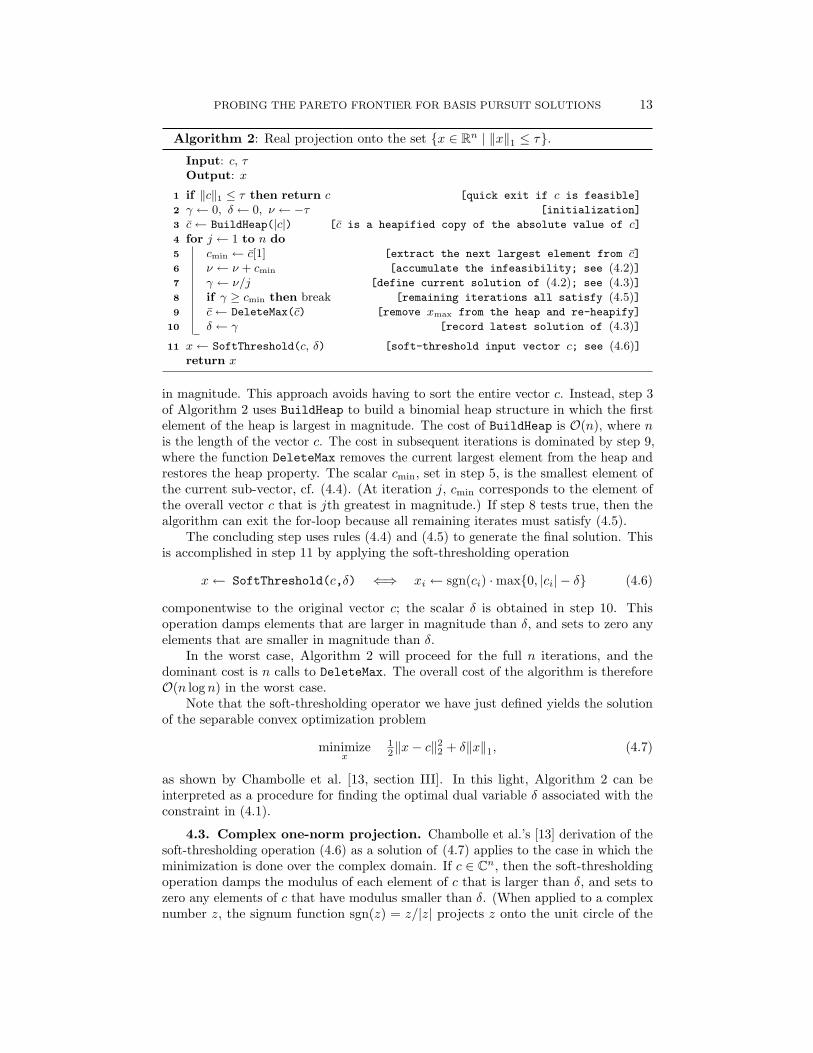
Algorithm 2: Real projection onto the set {x ∈ Rn | ‖x‖1 ≤ τ}.Input: c, τOutput: x

if ‖c‖1 ≤ τ then return c [quick exit if c is feasible]1

γ ← 0, δ ← 0, ν ← −τ [initialization]2

c← BuildHeap(|c|) [c is a heapified copy of the absolute value of c]3

for j ← 1 to n do4

cmin ← c[1] [extract the next largest element from c]5

ν ← ν + cmin [accumulate the infeasibility; see (4.2)]6

γ ← ν/j [define current solution of (4.2); see (4.3)]7

if γ ≥ cmin then break [remaining iterations all satisfy (4.5)]8

c← DeleteMax(c) [remove xmax from the heap and re-heapify]9

δ ← γ [record latest solution of (4.3)]10

x← SoftThreshold(c, δ) [soft-threshold input vector c; see (4.6)]11

return x

in magnitude. This approach avoids having to sort the entire vector c. Instead, step 3of Algorithm 2 uses BuildHeap to build a binomial heap structure in which the firstelement of the heap is largest in magnitude. The cost of BuildHeap is O(n), where nis the length of the vector c. The cost in subsequent iterations is dominated by step 9,where the function DeleteMax removes the current largest element from the heap andrestores the heap property. The scalar cmin, set in step 5, is the smallest element ofthe current sub-vector, cf. (4.4). (At iteration j, cmin corresponds to the element ofthe overall vector c that is jth greatest in magnitude.) If step 8 tests true, then thealgorithm can exit the for-loop because all remaining iterates must satisfy (4.5).

The concluding step uses rules (4.4) and (4.5) to generate the final solution. Thisis accomplished in step 11 by applying the soft-thresholding operation

x← SoftThreshold(c,δ) ⇐⇒ xi ← sgn(ci) ·max{0, |ci| − δ} (4.6)

componentwise to the original vector c; the scalar δ is obtained in step 10. Thisoperation damps elements that are larger in magnitude than δ, and sets to zero anyelements that are smaller in magnitude than δ.

In the worst case, Algorithm 2 will proceed for the full n iterations, and thedominant cost is n calls to DeleteMax. The overall cost of the algorithm is thereforeO(n log n) in the worst case.

Note that the soft-thresholding operator we have just defined yields the solutionof the separable convex optimization problem

minimizex

12‖x− c‖

22 + δ‖x‖1, (4.7)

as shown by Chambolle et al. [13, section III]. In this light, Algorithm 2 can beinterpreted as a procedure for finding the optimal dual variable δ associated with theconstraint in (4.1).

4.3. Complex one-norm projection. Chambolle et al.’s [13] derivation of thesoft-thresholding operation (4.6) as a solution of (4.7) applies to the case in which theminimization is done over the complex domain. If c ∈ Cn, then the soft-thresholdingoperation damps the modulus of each element of c that is larger than δ, and sets tozero any elements of c that have modulus smaller than δ. (When applied to a complexnumber z, the signum function sgn(z) = z/|z| projects z onto the unit circle of the


Algorithm 3: Complex projection onto the set {z ∈ Cn | ‖z‖1 ≤ τ}.Input: c, τOutput: z

r ← |c| [compute the componentwise modulus of c]1

r ← Pτ [r] [apply Algorithm 2; see (4.1)]2

foreach i = 1 to n doif ri > 0 then zi ← ci(ri/ri) [compute sgn(ci) · ri; see (4.6)]3

else zi ← 0 [the element ci was zero; keep it]4

return z

complex domain; by convention, sgn(0) = 0.) Thus, the thresholding operation on conly acts on the modula of each component, leaving the phases untouched.

We can use Algorithm 2 (projection of a real vector) to bootstrap an efficientalgorithm for projection of complex vectors. Algorithm 3 outlines this approach. First,the vector of modula r = (|c1| · · · |cn|) is computed (step 1), and then is projected ontothe (real) one-norm ball with radius τ (step 2). Next, the soft-thresholding operationof (4.6) is applied in steps 3–4.

The SPG method outlined in Algorithm 1 requires only an efficient procedurefor the projection onto the convex feasible set—the form of that convex set has noeffect on the rest of the algorithm. An important benefit of this is that, with the real-and complex-projection Algorithms 2 and 3, the SPG method applies equally well toproblems in the real and complex domains.

5. Implementation. The methods that we describe in this paper have beenimplemented as a single Matlab [38] software package called SPGL1. It implementsthe root-finding algorithm described in section 3 and the spectral projected-gradientalgorithm described in section 4; the latter is in fact the computational kernel.

The SPGL1 implementation is structured around major and minor iterations. Eachmajor iteration is responsible for determining the next element of the sequence {τk},and for invoking the SPG method described in Algorithm 1 to determine approximatevalues of φ(τk) and φ′(τk). For each major iteration k, there is a corresponding setof minor iterates converging to (xτk , rτk) that comprise the iterates of Algorithm 1.Unless the user can provide a good estimate for the solution τσ of (1.2), the root-findingalgorithm chooses τ0 = 0. This leads to an essentially “free” first major iterationbecause φ(0) = ‖b‖2 and φ′(0) = ‖ATb‖∞; with (3.1), it holds immediately that thenext Newton iterate τ1 = (σ − ‖b‖2)/‖ATb‖∞ exactly.

A small modification to Algorithm 1 is needed before we can implement theinexact Newton method of the outer iterations. Instead of using a fixed threshold δ, wecompare the duality-gap test in step 2 to the current relative error in satisfying (1.2).Thus, the (LSτ ) subproblem is solved to low accuracy during early major iterations(when τk in known only roughly), but more accurately as the error in satisfying (1.2)decreases. If only the solution of (LSτ ) is required, then a single call to Algorithm 1 ismade with δ held at some fixed value.

6. Numerical experiments. This section summarizes a series of numericalexperiments in which we apply SPGL1 to basis pursuit (BP), basis pursuit denoise(BPσ), and Lasso (LSτ ) problems. The experiments include a selection of sixteenrelevant problems from the Sparco [2] collection of test problems. The chosen problemsare all real-valued and suited to one-norm regularization. We exclude problems thatare complex-valued, that are better suited to total-variation regularization, or that


Table 6.1: Key to symbols used in tables 6.2–6.4

m, n number of rows and columns of A‖b‖2 two-norm of the right-hand-side vector‖r‖2 two-norm of the computed residual‖x‖1 one-norm of the computed solutionnnz(x) number of nonzeros in the computed solution; see (6.1)nMat total number of matrix-vector products with A and AT

f solver failed to return a feasible solutiont solver failed to converge within allotted CPU time

Table 6.2: The Sparco test problems used

Problem ID m n ‖b‖2 operator

blocksig 2 1024 1024 7.9e+1 waveletblurrycam 701 65536 65536 1.3e+2 blurring, waveletblurspike 702 16384 16384 2.2e+0 blurringcosspike 3 1024 2048 1.0e+2 DCTdcthdr 12 2000 8192 2.3e+3 restricted DCTfinger 703 11013 125385 5.5e+1 2D curveletgcosspike 5 300 2048 8.1e+1 Gaussian ensemble, DCTjitter 902 200 1000 4.7e−1 DCTp3poly 6 600 2048 5.4e+3 Gaussian ensemble, waveletseismic 901 41472 480617 1.1e+2 2D curveletsgnspike 7 600 2560 2.2e+0 Gaussian ensemblesoccer1 601 3200 4096 5.5e+4 binary ensemble, waveletspiketrn 903 1024 1024 5.7e+1 1D convolutionsrcsep1 401 29166 57344 2.2e+1 windowed DCTsrcsep2 402 29166 86016 2.3e+1 windowed DCTyinyang 603 1024 4096 2.5e+1 wavelet

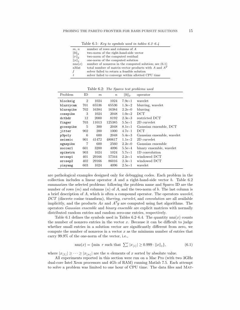
are pathological examples designed only for debugging codes. Each problem in thecollection includes a linear operator A and a right-hand-side vector b. Table 6.2summarizes the selected problems: following the problem name and Sparco ID are thenumber of rows (m) and columns (n) of A, and the two-norm of b. The last column isa brief description of A, which is often a compound operator. The operators wavelet,DCT (discrete cosine transform), blurring, curvelet, and convolution are all availableimplicitly, and the products Ax and ATy are computed using fast algorithms. Theoperators Gaussian ensemble and binary ensemble are explicit matrices with normallydistributed random entries and random zero-one entries, respectively.

Table 6.1 defines the symbols used in Tables 6.2–6.4. The quantity nnz(x) countsthe number of nonzero entries in the vector x. Because it can be difficult to judgewhether small entries in a solution vector are significantly different from zero, wecompute the number of nonzeros in a vector x as the minimum number of entries thatcarry 99.9% of the one-norm of the vector, i.e.,

nnz(x) = {min r such that∑ri |xbic| ≥ 0.999 · ‖x‖1}, (6.1)

where |xb1c| ≥ · · · ≥ |xbnc| are the n elements of x sorted by absolute value.All experiments reported in this section were run on a Mac Pro (with two 3GHz

dual-core Intel Xeon processors and 4Gb of RAM) running Matlab 7.5. Each attemptto solve a problem was limited to one hour of CPU time. The data files and Mat-


Table 6.3: Basis pursuit denoise comparisons

Homotopy SPGL1

Problem ‖r‖2 ‖x‖1 nnz(x) nMat ‖r‖2 ‖x‖1 nnz(x) nMat

blocksig 7.9e+0 3.8e+2 64 230 7.9e+0 3.8e+2 64 217.9e−2 4.5e+2 71 246 7.9e−2 4.5e+2 71 22

blurrycam 1.3e+1 1.2e+3 298 1290 1.3e+1 1.2e+3 299 34t t t t 1.3e−1 9.1e+3 59010 2872

blurspike 2.2e−1 1.5e+2 175 770 2.2e−1 1.5e+2 181 264t t t t 2.3e−3 3.4e+2 15324 3238

cosspike 1.0e+1 1.3e+2 2 8 1.0e+1 1.3e+2 2 311.0e−1 2.2e+2 113 496 1.0e−1 2.2e+2 113 77

dcthdr 2.3e+2 3.7e+4 133 568 2.3e+2 3.7e+4 133 342.3e+0 4.4e+4 266 1436 2.3e+0 4.4e+4 266 114

finger t t t t 5.5e+0 4.4e+3 7968 252t t t t 5.5e−2 5.5e+3 13564 1128

gcosspike 8.1e+0 1.3e+2 4 20 8.1e+0 1.3e+2 4 348.1e−2 1.8e+2 94 882 8.1e−2 1.8e+2 112 434

jitter 4.7e−2 1.6e+0 3 12 4.7e−2 1.6e+0 3 204.7e−4 1.7e+0 3 12 5.3e−4 1.7e+0 3 30

p3poly 5.4e+2 1.4e+3 155 708 5.4e+2 1.4e+3 155 688.5e+1 1.7e+3 494 3364 5.4e+0 1.7e+3 518 478

seismic 1.1e+1 2.8e+3 554 4172 1.1e+1 2.8e+3 646 141t t t t 1.1e−1 3.9e+3 14806 709

sgnspike 2.2e−1 1.8e+1 20 80 2.2e−1 1.8e+1 20 302.2e−3 2.0e+1 20 80 2.2e−3 2.0e+1 20 44

soccer1 5.5e+3 5.5e+1 4 16 5.5e+3 5.5e+1 4 145.5e+1 3.1e+2 769 3460 5.5e+1 3.1e+2 1073 1250

spiketrn 5.7e+0 1.0e+1 51 310 5.7e+0 1.0e+1 73 6175.7e−2 1.3e+1 35 480 5.7e−2 1.3e+1 418 4761

srcsep1 t t t t 2.2e+0 8.0e+2 7838 160t t t t 2.2e−2 1.0e+3 22428 1125

srcsep2 t t t t 2.3e+0 8.6e+2 8652 246t t t t 2.3e−2 1.1e+3 25359 947

yinyang 2.5e+0 1.8e+2 153 668 2.5e+0 1.8e+2 153 442.5e−2 2.6e+2 881 4332 2.6e−2 2.6e+2 969 396

lab scripts used to generate all of the numerical results presented in the followingsubsections can be obtained at http://www.cs.ubc.ca/labs/scl/spgl1.

6.1. Basis pursuit denoise. For each of the sixteen test problems listed inTable 6.2, we generate two values of σ: σ1 = 10−1‖b‖2 and σ2 = 10−3‖b‖2. We thushave a total of thirty-two test problems of the form (BPσ) to which we apply SPGL1.

As a benchmark, we also give results for the SolveLasso solver available withinthe SparseLab package, which we apply in its “lasso” mode (there is also an optional“lars” mode). In this mode, SolveLasso applies the homotopy method described insection 1.4 to solve (QPλ) for all values of λ ≥ 0. The SolveLasso solver beginswith λ = ‖ATb‖∞, which has the corresponding trivial solution xλ = 0, and reducesλ in stages so that the corresponding sequence of solutions xλ have exactly oneadditional nonzero entry each. The norm of the residual rλ ≡ b − Axλ decreases

http://www.cs.ubc.ca/labs/scl/spgl1


monotonically. We set the parameters resStop = σ and lamStop = 0, which togetherrequire SolveLasso to iterate until ‖rλ‖2 ≤ σ and xλ is therefore feasible for (BPσ).

Table 6.3 summarizes the results. The rows in each two-row block correspond toinstances of the same test problem (i.e., the same A and b) with parameters σ1 andσ2. The SparseLab results are shown under the column head “Homotopy.” SparseLabdid not obtain accurate results for nine problems—blurrycam(2), blurspike(2),finger(1,2), seismic(2), srcsep1(1,2), and srcsep2(1,2) (the numbers in paren-theses refer to the particular problem instance)—because it failed to converge withinthe allotted time. For these problems, the number of nonzero elements in the currentsolution vector grows very large. SparseLab maintains a dense factorization of thesubmatrix of A corresponding to these indices, and the time needed to update thisfactorization can grow very large as the nonzero index set grows. In contrast, thehomotopy method can be very efficient when the number of nonzeros in the solution issmall. SPGL1 succeeds in obtaining solutions to every problem instance, and we notethat the memory requirements are constant throughout all iterations.

The quadratically constrained solver l1qc newton, available within the `1-magicsoftware package [9], is also applicable to the problem (BPσ) when A is only availableas an operator. However, we do not include the results obtained with `1-magic becauseit failed on all but ten of the thirty-two test problems—the solver either reported“stuck on cone iterations” (i.e., it could not compute a sufficiently accurate searchdirection within a predetermined number of conjugate-gradient iterations) or failedto return a solution within the allotted one hour of CPU time. Other quadraticallyconstrained solvers such as MOSEK and SeDuMi are not applicable because they allrequire A as an explicit matrix.

6.2. Basis pursuit. The basis pursuit (BP) problem can be considered to be aspecial case of (BPσ) in which σ = 0. In this section we give the results of experimentsthat show that SPGL1 can be an effective algorithm for solving (BP). We apply SPGL1

to sixteen (BP) problems generated from the test set shown in Table 6.2.As benchmarks, we also give results of applying the solvers SolveLasso and

SolveBP, which are both available within the SparseLab package. For SolveLasso weagain use its “lasso” mode and set the parameters resStep = 10−4 and lamStep = 0.We use default parameters for SolveBP. Note that SolveBP applies the interior-pointcode PDCO [44] to a linear programming reformulation of (BP) and only requiresmatrix-vector products with A and AT.

The top half of Table 6.4 lists the norms of the computed norms and residuals,and the bottom half lists the sparsity of the computed solutions and the number ofmatrix-vector products required. Both PDCO and the homotopy approach failed toconverge within the allotted one hour of CPU time on problems blurrycam, finger,seismic, and soccer1. Homotopy had the same failure for problems blurryspike,srcsep1, and srcsep2, and in addition it failed to return feasible solutions to withinthe required tolerance for p3poly and yinyang. SPGL1 succeeded in all cases. Again,for problems that have very sparse solutions, homotopy can be much more efficientthan SPGL1; for example, see problems gcosspike and spiketrn in Table 6.4.

Figure 6.1 shows the results of applying SPGL1 to problem seismic. The corruptedseismic image in Figure 6.1(a) is missing 35% of its traces (i.e., measurements); theinterpolated image in Figure 6.1(b) is computed from the solution of (BP), where A isa restricted curevelet transform. Figure 6.1(c) shows a graph of the Pareto curve forthis problem, and the trajectory that SPGL1 follows to arrive at a (BP) solution.


Table 6.4: Basis pursuit comparisons

PDCO Homotopy SPGL1

Problem ‖r‖2 ‖x‖1 ‖r‖2 ‖x‖1 ‖r‖2 ‖x‖1

blocksig 3.3e−04 4.5e+02 1.0e−04 4.5e+02 2.0e−14 4.5e+02blurrycam t t t t 9.9e−05 1.0e+04blurspike 9.1e−03 3.4e+02 t t 9.9e−05 3.5e+02cosspike 1.6e−04 2.2e+02 1.0e−04 2.2e+02 8.6e−05 2.2e+02dcthdr 1.3e−05 4.4e+04 5.5e−08 4.4e+04 4.9e−05 4.4e+04finger t t t t 8.2e−05 5.5e+03gcosspike 1.9e−05 1.8e+02 1.0e−04 1.8e+02 9.9e−05 1.8e+02jitter 1.3e−05 1.8e+00 1.0e−04 1.7e+00 5.3e−05 1.7e+00p3poly 4.6e−02 1.7e+03 8.5e+01f 1.8e+03 9.5e−05 1.7e+03seismic t t t t 8.6e−05 3.9e+03sgnspike 9.3e−06 2.0e+01 1.0e−04 2.0e+01 8.0e−05 2.0e+01soccer1 t t t t 1.0e−04 4.2e+02spiketrn 3.6e−03 1.3e+01 1.0e−04 1.3e+01 9.9e−05 1.3e+01srcsep1 8.2e−03 1.1e+03 t t 8.6e−05 1.1e+03srcsep2 5.5e−03 1.1e+03 t t 1.0e−04 1.1e+03yinyang 1.4e−03 2.6e+02 2.8e−03f 4.7e+02 9.6e−05 2.6e+02

PDCO Homotopy SPGL1

Problem nnz(x) nMat nnz(x) nMat nnz(x) nMat

blocksig 71 703 71 246 71 21blurrycam t t t t 62756 8237blurspike 15513 59963 t t 15585 5066cosspike 119 2471 115 500 115 111dcthdr 270 79911 270 1436 270 294finger t t t t 13333 3058gcosspike 335 14755 59 934 195 2535jitter 678 43 3 12 3 38p3poly 559 145053 503f 3882 526 3047seismic t t t t 22816 3871sgnspike 1018 131 20 80 20 56soccer1 t t t t 3805 63233spiketrn 30 1169 12 480 12 26406srcsep1 40950 78385 t t 24641 2881srcsep2 67029 47109 t t 26653 2432yinyang 1733 34667 981f 9680 1031 1198

6.3. The Lasso and quadratic programs. The main goal of this work is toprovide an efficient algorithm for (BPσ). But for interest, we show here how SPGL1

can also be used to efficiently solve a single instance of the Lasso problem (LSτ ).This corresponds to solving a single instance of (QPλ) where λ is set to the Lagrangemultiplier of the Lasso constraint.

In Figure 6.2 we compare the performance and computed solutions of the solversGPSR (version of August 2007) [27], L1LS [34], PDCO [44], and SPGL1, applied to theproblems dcthdr and srcsep1. For each of these two problems we generate fifty valuesof λ and τ for which the solutions of (QPλ) and (LSτ ) coincide, and thus generate fiftytest cases each of types (QPλ) and (LSτ ). We apply GPSR, L1LS, and PDCO to each(QPλ) test case, and apply SPGL1 to each (LSτ ) test case.

Plots (a) and (c) in Figure 6.2 show the Pareto curves for problems dcthdr andsrcsep1, and the norms of computed solutions versus the norms of the correspondingresiduals. (Note that these curves are plotted on a semi-log scale, and thus are not


Trace #

Tim

e

50 100 150 200 250

(a) Image with missing traces

Trace #

50 100 150 200 250

(b) Interpolated image

0 0.5 1 1.5 20

50

100

150

200

250

one−norm of solution (x104)

two

−n

orm

of

resi

du

al

Pareto curveSolution path

(c) Pareto curve and solution path

Fig. 6.1: Corrupted and interpolated images for problem seismic. Graph (c) shows thePareto curve and the solution path taken by SPGL1.

convex.) For each point in the left-hand figure, the points in the right-hand figure givethe number of matrix-vector products required to obtain the corresponding solution.Points on the Pareto curve are accurate solutions; inaccurate solutions lie above thecurve, indicating that they do not solve the corresponding problem (QPλ) or (LSτ ).

In Figure 6.2(a), almost all points lie on the Pareto curve, and thus most of thecomputed solutions are accurate. The corresponding points in Figure 6.2(b) indicatethat SPGL1 and GPSR use only a small fraction of the matrix-vector products requiredby PDCO and L1LS, which are second-order methods. We note that solutions forproblem dcthdr can range over four orders of magnitude, and yet the first-ordermethods appear not to be affected by this poor scaling.

In Figure 6.2(c), the computed solutions returned by PDCO and GPSR areprogressively worse as λ tends to zero (and the one-norm of the solution increases).Interestingly, L1LS consistently yields very accurate solutions for all values of λ;however, as might be expected of an interior-point method based on a conjugate-


0 1 2 3 4

x 104

102

103


two−

norm

of r

esid

ual

Pareto curveGPSRL1LSPDCOSPGL1

(a) dcthdr: solution quality

0 1 2 3 4

x 104

100

101

102

103

104

105


num

ber

mat

rix−

vect

or p

rodu

cts

(b) dcthdr: solver performance

0 200 400 600 800 1000

10−1

100

101


two−

norm

of r

esid

ual

Pareto curveGPSRL1LSPDCOSPGL1

(c) srcsep1: solution quality

0 200 400 600 800 100010

0

101

102

103

104

105


num

ber

mat

rix−

vect

or p

rodu

cts

(d) srsecp1: solver performance

Fig. 6.2: Performance of solvers on equivalent (QPλ) and (LSτ ) problems. The top row isfor problem dcthdr and the bottom row is for problem srcsep1. The plots on the left showthe norms of the computed residuals and solutions for fifty parameter values; the plots on theright give the corresponding number of required matrix-vector products. Note that the curvesin the left-hand figures are not convex because they are plotted on a semi-log scale.

gradient linear solver, it can require many matrix-vector products.It may be progressively more difficult to solve (QPλ) as λ → 0 because the

regularizing effect from the one-norm term tends to become negligible, and there is lesscontrol over the norm of the solution. In contrast, the (LSτ ) formulation is guaranteedto maintain a bounded solution norm for all values of τ .

6.4. Sampling the Pareto curve. In situations where little is known aboutthe noise level σ, it may be useful to visualize the Pareto curve in order to understandthe trade-offs between the norms of the residual and of the solution. In this sectionwe aim to obtain good approximations to the Pareto curve for cases in which it isprohibitively expensive to compute it in its entirety.

We test two approaches for interpolation through a small set of samples i = 1, . . . , k.In the first, we generate a uniform distribution of parameters λi = (i/k)‖ATb‖∞, andsolve the corresponding problems (QPλi). In the second, we generate a uniform distri-bution of parameters σi = (i/k)‖b‖2, and solve the corresponding problems (BPσi).


0 200 400 600 800 1000 12000

5

10

15

20


two−

norm

of r

esid

ual

Pareto curveσ−based approximationλ−based approximationσ−based samplesλ−based samples

(a) srcsep1: linear extrapolation

0 200 400 600 800 1000 12000

5

10

15

20


two−

norm

of r

esid

ual

(b) srcsep1: quadratic extrapolation

0 50 100 150 2000

10

20

30

40

50

60

70

80


two−

norm

of r

esid

ual

(c) gcosspike: linear extrapolation

0 50 100 150 2000

10

20

30

40

50

60

70

80


two−

norm

of r

esid

ual

(d) gcosspike: pure interpolation

Fig. 6.3: Extrapolation of the Pareto curve based on samples obtained by solving (BPσ) or(QPλ), respectively, at uniformly spaced values of σ and λ. Graphs (a)–(c) show results forlinear and quadratic extrapolation; graph (d) shows the gains from using the τBP point andpure interpolation

We leverage the convexity and differentiability of the Pareto curve to approximate itwith piecewise cubic polynomials that match function and derivative values at eachend. When a non-convex fit is detected, we switch to a quadratic interpolation on therelevant interval and match derivative information only at one end. Extrapolationis based on only the function and derivative values of the last sample point. Thisnaturally suggests using a linear extrapolation which, due to convexity of the Paretocurve, is guaranteed never to overestimate the curve or the value of τBP. Alternatively,we can use quadratic extrapolation through the last point and require the minimum ofthe extrapolation to coincide exactly with the horizontal axis. This approach works wellwhen the Pareto curve is nearly quadratic at the end, but it is likely to overestimatethe curve in other cases. Forming linear combinations of the two functions provides abalanced extrapolation that ranges from conservative to risky.

Figure 6.3 illustrates an approximation of the Pareto curve that is based on a smallnumber of samples. Note that the sampling based on σ gives a better distribution ofpoints on the curve as compared to sampling based on λ; this was observed for allproblems tested and coincides with the observations made by Das and Dennis [19] andLeyffer [35]. For the curves shown in plots (a) and (b), the σ-based samples clearly


lead to better approximations. For Pareto curves that are nearly linear, such as thoseshown in plots (c) and (d), there is little to no difference between the σ- and λ-basedsamples. For this test problem, the relatively sharp bend near the end of the curvemakes it difficult to reconstruct the curve accurately unless σ or λ is sampled morefinely, or unless the BP solution is sampled as illustrated in (d). An adaptive approach,such as that proposed by Leyffer [35], could lead to more accurate sampling.

7. Looking ahead. Our original motivation for developing the method proposedin this paper is its usefulness for inpainting applications in seismic imaging, where theproblem sizes can stretch into millions of variables [32]. We are currently developingan out-of-core implementation of SPGL1 based on the SlimPy [33] package.

We are also considering an extension of the root-finding approach for solving thenonlinear regularization problem

minimizex

f(x) subject to ‖Ax− b‖2 ≤ σ,

where f is a convex nonlinear function. This may open the door to applying the Paretoroot-finding approach to other applications.

8. Acknowledgments. The authors are grateful to Chen Greif, Gilles Hennen-fent, Felix Herrmann, Michael Saunders, and Ozgur Yılmaz for their valuable input.We extend sincere thanks to two anonymous referees for their thoughtful suggestions.

REFERENCES

[1] J. Barzilai and J. M. Borwein, Two-point step size gradient methods, IMA J. Numer. Anal.,8 (1988), pp. 141–148.

[2] E. van den Berg, M. P. Friedlander, G. Hennenfent, F. Herrmann, R. Saab, andO. Yılmaz, Sparco: A testing framework for sparse reconstruction, Tech. Rep. TR-2007-20,Dept. Computer Science, University of British Columbia, Vancouver, October 2007.

[3] D. P. Bertsekas, Nonlinear Programming, Athena Scientific, Belmont, MA, second ed., 1999.[4] , Convex Analysis and Optimization, Athena Scientific, Belmont, MA, 2003.[5] E. G. Birgin, J. M. Martınez, and M. Raydan, Nonmonotone spectral projected gradient

methods on convex sets, SIAM J. Optim., 10 (2000), pp. 1196–1211.[6] , Inexact spectral projected gradient methods on convex sets, IMA J. Numer. Anal., 23

(2003), pp. 1196–1211.[7] A. Bjorck, Numerical Methods for Least Squares Problems, Society for Industrial Mathematics,

1996.[8] S. Boyd and L. Vandenberghe, Convex Optimization, Cambridge University Press, Cambridge,

UK, 2004.[9] E. Candes and J. Romberg, `1-magic. http://www.l1-magic.org/, 2007.

[10] E. J. Candes, J. Romberg, and T. Tao, Robust uncertainty principles: exact signal recon-struction from highly incomplete frequency information, IEEE Trans. Inform. Theory, 52(2006), pp. 489–509.

[11] , Stable signal recovery from incomplete and inaccurate measurements, Comm. Pure Appl.Math., 59 (2006), pp. 1207–1223.

[12] E. J. Candes and T. Tao, Near-optimal signal recovery from random projections: Universalencoding strategies?, IEEE Trans. Inform. Theory, 52 (2006), pp. 5406–5425.

[13] A. Chambolle, R. De Vore, N.-Y. Lee, and B. Lucier, Nonlinear wavelet image processing:variational problems, compression, and noise removal through wavelet shrinkage, IEEETrans. Image Proc., 7 (1998), pp. 319–335.

[14] S. S. Chen, D. L. Donoho, and M. A. Saunders, Atomic decomposition by basis pursuit,SIAM J. Sci. Comput., 20 (1998), pp. 33–61.

[15] , Atomic decomposition by basis pursuit, SIAM Rev., 43 (2001), pp. 129–159.[16] ILOG CPLEX. Mathematical programming system, http://www.cplex.com, 2007.[17] Y. Dai, W. W. Hager, K. Schittkowski, and H. Zhang, The cyclic Barzilai-Borwein method

for unconstrained optimization, IMA J. Numer. Anal., 7 (2006), pp. 604–627.

http://www.l1-magic.org/

http://www.cplex.com


[18] Y.-H. Dai and R. Fletcher, Projected Barzilai-Borwein methods for large-scale box-constrainedquadratic programming, Numer. Math., 100 (2005), pp. 21–47.

[19] I. Das and J. E. Dennis, A closer look at drawbacks of minimizing weighted sums of objectivesfor Pareto set generation in multicriteria optimization problems, Structural Optim., 14(1997), pp. 63–69.

[20] I. Daubechies, M. Fornasier, and I. Loris, Accelereated projected gradient method for linearinverse problems with sparsity constraints, J. Fourier Anal. Appl., (2007). To appear.

[21] A. Dax, On regularized least norm problems, SIAM J. Optim., 2 (1992), pp. 602–618.[22] R. S. Dembo, S. C. Eisenstat, and T. Steihaug, Inexact Newton methods, SIAM J. Numer.

Anal., 19 (1982), pp. 400–408.[23] D. L. Donoho, Compressed sensing, IEEE Trans. Inform. Theory, 52 (2006), pp. 1289–1306.[24] D. L. Donoho, For most large underdetermined systems of linear equations the minimal `1-norm

solution is also the sparsest solution, Comm. Pure Appl. Math., 59 (2006), pp. 797–829.[25] D. L. Donoho and Y. Tsaig, Fast solution of l1-norm minimization problems when the solution

may be sparse. http://www.stanford.edu/~tsaig/research.html, October 2006.[26] B. Efron, T. Hastie, I. Johnstone, and R. Tibshirani, Least angle regression, Ann. Statist.,

32 (2004), pp. 407–499.[27] M. Figueiredo, R. Nowak, and S. Wright, Gradient projection for sparse reconstruction:

Application to compressed sensing and other inverse problems, Selected Topics in Sig. Proc.,IEEE J., 1 (2007), pp. 586–597.

[28] M. P. Friedlander and M. A. Saunders, Discussion: the Dantzig selector: statisticalestimation when p is much larger than n, Annals Statist., 35 (2007), pp. 2385–2391.

[29] P. C. Hansen, Rank-Deficient and Discrete Ill-Posed Problems, Society of Industrial andApplied Mathematics, Philadelphia, 1998.

[30] P. C. Hansen and D. P. O’Leary, The use of the L-curve in the regularization of discreteill-posed problems, SIAM J. Sci. Comput., 14 (1993), pp. 1487–1503.

[31] G. Hennenfent and F. J. Herrmann, Sparseness-constrained data continuation with frames:Applications to missing traces and aliased signals in 2/3-D, in SEG International Expositionand 75th Annual Meeting, 2005.

[32] , Simply denoise: wavefield reconstruction via coarse nonuniform sampling, tech. rep.,UBC Earth & Ocean Sciences, August 2007.

[33] F. Herrmann and S. Ross-Ross, SlimPy: A Python interface to Unix-like pipe based linearoperators. http://slim.eos.ubc.ca/SLIMpy, 2007.

[34] S.-J. Kim, K. Koh, M. Lustig, S. Boyd, and D. Gorinevsky, An interior-point method forlarge-scale `1-regularized least squares, Selected Topics in Sig. Proc., IEEE J., 1 (2007),pp. 606–617.

[35] S. Leyffer, A note on multiobjective optimization and complementarity constraints, PreprintANL/MCS-P1290-0905, Mathematics and Computer Science Division, Argonne NationalLaboratory, Illinois, September 2005.

[36] M. Lustig, D. Donoho, and J. Pauly, Sparse MRI: The application of compressed sensingfor rapid MR imaging, Magnetic Resonance in Medicine, 58 (2007), pp. 1182–1195.

[37] M. Lustig, D. L. Donoho, J. M. Santos, and J. M. Pauly, Compressed sensing MRI, 2007.Submitted to IEEE Signal Processing Magazine.

[38] MathWorks, MATLAB User’s Guide, The MathWorks, Inc., Natick, MA, 1992.[39] Mathematical programming system, http://www.mosek.com, 2007.[40] J. Nocedal and S. J. Wright, Numerical Optimization, Springer, New York, second ed., 2006.[41] M. R. Osborne, B. Presnell, and B. A. Turlach, A new approach to variable selection in

least squares problems, IMA J. Numer. Anal., 20 (2000), pp. 389–403.[42] M. R. Osborne, B. Presnell, and B. A. Turlach, On the LASSO and its dual, J. Comput.

Graph. Stat., 9 (2000), pp. 319–337.[43] R. T. Rockafellar, Convex Analysis, Princeton University Press, Princeton, 1970.[44] M. A. Saunders, PDCO. Matlab software for convex optimization, http://www.stanford.

edu/group/SOL/software/pdco.html, 2005.[45] J. F. Sturm, Using SeDuMi 1.02, a Matlab toolbox for optimization over symmetric cones

(updated for Version 1.05), tech. rep., Department of Econometrics, Tilburg University,Tilburg, The Netherlands, August 1998 – October 2001.

[46] R. Tibshirani, Regression shrinkage and selection via the Lasso, J. Roy. Statist. Soc. B., 58(1996), pp. 267–288.

[47] A. N. Tikhonov and V. Y. Arsenin, Solutions of Ill-Posed Problems, V. H. Winston and Sons,Washington, D.C., 1977. Translated from Russian.

[48] J. A. Tropp, Just relax: Convex programming methods for identifying sparse signals in noise,IEEE Trans. Inform. Theory, 52 (2006), pp. 1030–1051.

http://www.stanford.edu/~tsaig/research.html

http://slim.eos.ubc.ca/SLIMpy

http://www.mosek.com

http://www.stanford.edu/group/SOL/software/pdco.html

http://www.stanford.edu/group/SOL/software/pdco.html

Documents

1. Basis pursuit denoise. Ax b m n - Optimization Online · 1 subject to kAx bk 2 ˙; where the positive parameter ˙is an estimate of the noise level in the data. The case ˙= 0