Embed Size (px)
Citation preview

1
Bayesian Restoration Using a New Nonstationary
Edge-Preserving Image Prior
Giannis K. Chantas, Nikolaos P. Galatsanos, and Aristidis C. Likas
IEEE Transactions on Image Processing, Vol. 15, No. 10, October 2006
2
Outline
Review of Markov random field (MRF) for signal restoration problem
Bayesian restoration using a new non-stationary
edge-preserving image prior

3
MAP formulation for signal restoration problem
Noisy signal d Restored signal f

4
MAP formulation for signal restoration problem
The problem of the signal restoration could be modeled as the MAP estimation problem, that is,
arg max{ ( | )}
By Baye's rule:
arg max{ ( | ) ( )}
:
:
f
f
f p f d
f p d f p f
f Unknown data
d Observed data
(Prior model)
(Observation
model)
5
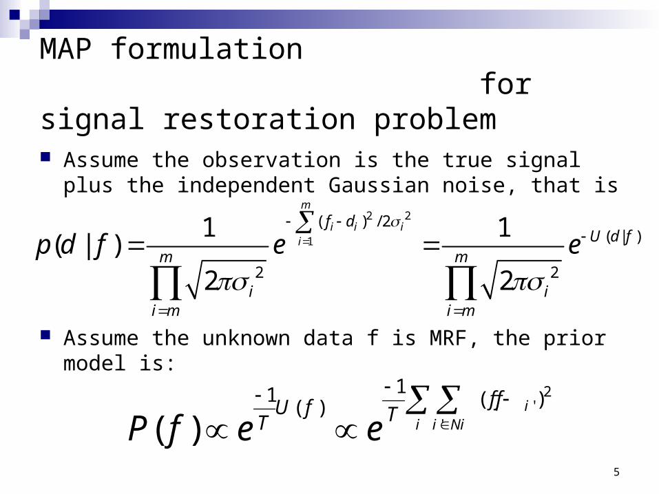
MAP formulation for signal restoration problem
Assume the observation is the true signal plus the independent Gaussian noise, that is
Assume the unknown data f is MRF, the prior model is:
2 2
1
( ) / 2( | )
2 2
1 1( | )
2 2
m
i i ii
f dU d f
m m
i ii m i m
p d f e e
2'
'
11 ( )( )( )
i ii i Ni
f fU f TTP f e e

6
MAP formulation for signal restoration problem
Substitute above information into the MAP estimator, we could get:
22
121 1
arg max{ ( | )} arg min{ ( | ) ( )}
( )arg min{ ( ) }
2
f f
m mi i
f i ii i
f p f d U d f U f
f df f
Observation model (Similarity measure)
Prior model (Reconstruction constrain, Regularization)

7
MAP formulation for signal restoration problem
From the potential function point of view:
2
212
1 1
( )arg min{ ( ) }
2
m mi i
f i ii i
f df f f
The edge region is blurred due to the improper design of the prior model

8
MRF with pixel process and line process (Geman and Geman, 1984)
Lattice of pixel site: SP Labeling value: fi
p (real value)
Lattice of line site: SE Labeling value: fii’
E (only 0 or 1)Compound MRF
2' ' '
'
( , ) ( ) (1 )P
P E P P E Ei i ii ii
i Nii S
U f f f f f f
Prior model with indicator (Line process)

9
MRF with nonstationary image prior (G.K. Chantas, N.P. Galatsanos and A.C. Likas, 2006)
From image modeling point of view, the binary nature (0 or 1) of the line process (Previous prior model) is insufficient to capture the image variations
Edge pattern 1
Edge pattern 2
Edge pattern 2 is more sharper than edge pattern 1

10
MRF with nonstationary image prior (G.K. Chantas, N.P. Galatsanos and A.C. Likas, 2006)
A linear imaging model is assumed in this paper, that is:
-1
where
: Observation (Nx1 vector)
:NxN convolution matrix
: Gassian noise with pdf (0, )
:
arg max{ ( | )} arg max{ ( | ) ( )} f f
g H f n
g
H
n N I
Goal
f p f g p g f p f
������������������������������������������
��������������
����������������������������������������������������������������������

11
MRF with nonstationary image prior (G.K. Chantas, N.P. Galatsanos and A.C. Likas, 2006)
For the image prior model, they assume the first order difference of the image f in four direction, 0o, 90o, 45o, 135o, respectively, are given by
f(i-1,j-1) f(i-1,j) f(i-1,j+1)
f(i,j-1) f(i,j) f(i,j+1)
f(i+1,j-1)
f(i+1,j) f(i+1,j+1)
A 3x3 image patch; f(i,j): Intensity at location (i,j)

12
MRF with nonstationary image prior (G.K. Chantas, N.P. Galatsanos and A.C. Likas, 2006)
The previous equation can be also written in matrix vector form for the entire image, that is
1 2
1
[ ..... ] , 1, 2,3, 4
where
: Difference operator for image f
(0, ( ) ) and is a parameter of the model
(Generalization of line process )
k k k TN
k k ki i i
kk
k
k and
N a a
Q f
Q
����������������������������

13
MRF with nonstationary image prior (G.K. Chantas, N.P. Galatsanos and A.C. Likas, 2006)
For convenience, author introduces the following notation
1 2
1 2 4
1 2 3 4
1 2 3 4
1 2 3 4
{ , ,..... }
{ , ,..... }
[ , , , ]
[ , , , ]
[( ) , ( ) , ( ) , ( ) ]
k k k kN
T
T
T T T T T
A diag a a a
A diag A A A
a a a a a
Q Q Q Q Q

14
MRF with nonstationary image prior (G.K. Chantas, N.P. Galatsanos and A.C. Likas, 2006)
Assume the residual εik in each direction and at each
pixel location are independent. Then, the joint density for the residuals is Gaussian and is given as:

15
MRF with nonstationary image prior (G.K. Chantas, N.P. Galatsanos and A.C. Likas, 2006)
We could get the pdf of image f by using the fact that:
Then we have:
Q f ��������������
Over-parameterization occurs of the proposed model !

16
MRF with nonstationary image prior (G.K. Chantas, N.P. Galatsanos and A.C. Likas, 2006)
To overcome the over-parameterization problem, the author views ai
k as a random variable instead of parameter and introduces Gamma hyper-prior for it
Where lk and mk are parameters of the hyper-prior

17
MRF with nonstationary image prior (G.K. Chantas, N.P. Galatsanos and A.C. Likas, 2006)
More on Gamma hyper-prior aik
2
[ ]
[ ]
k
ki
ki
if l
E a
Var a
1
[ ] (2 )
[ ] 0
k
ki k
ki
if l
E a m
Var a
Stationary prior Non-stationary prior
Pdf:

18
MRF with nonstationary image prior (G.K. Chantas, N.P. Galatsanos and A.C. Likas, 2006)
MAP estimation – Maximize p(.) is equivalent to minimize JMAP

19
MRF with nonstationary image prior (G.K. Chantas, N.P. Galatsanos and A.C. Likas, 2006)
Bayesian algorithm : We are interested in true value of f instead of ai
k – Marginalize aik for solution finding, that is
The image is estimated by finding the mode of above pdf
( , ; , , ) ( , , ; , , )p g f B m l p g f a B m l da
* arg max ( , ; , , )f
f p g f B m l

20
MRF with nonstationary image prior (G.K. Chantas, N.P. Galatsanos and A.C. Likas, 2006)
Definition for improvement signal to noise ration (ISNR)

21
Original image MAP non-stationary, ISNR:5.63 dB, l=2.2
Wiener filter, ISNR:3.2dB
Bayesian non-stationary, ISNR:5.22 dB, l=2.2
CLS, ISNR:4.65dBDegraded image

22