Embed Size (px)
Citation preview
1
Biased 2-b trees (Bent, Sleator, Tarjan 1980)
2
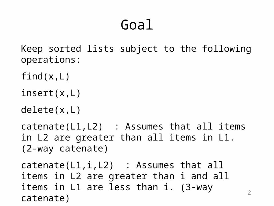
Goal
Keep sorted lists subject to the following operations:
find(x,L)
insert(x,L)
delete(x,L)
catenate(L1,L2) : Assumes that all items in L2 are greater than all items in L1. (2-way catenate)
catenate(L1,i,L2) : Assumes that all items in L2 are greater than i and all items in L1 are less than i. (3-way catenate)
split(x,L) : returns two or three lists. One with all item less than x, the other with all items greater than x, and the third with x if its in L.
3
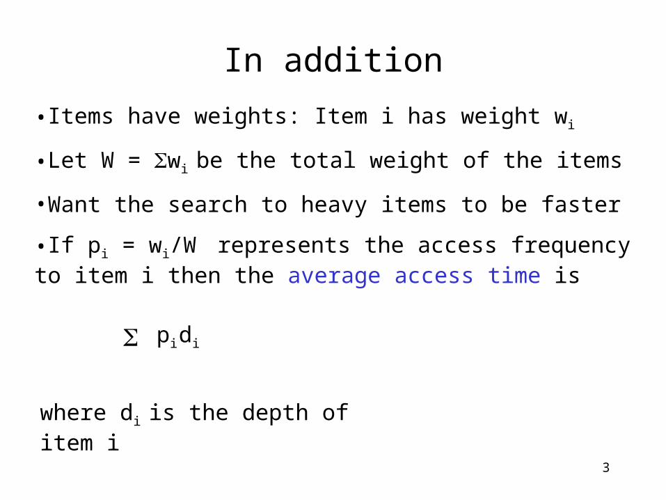
In addition
•Items have weights: Item i has weight wi
•Let W = wi be the total weight of the items
•Want the search to heavy items to be faster
•If pi = wi/W represents the access frequency to item i then the average access time is
pi di
where di is the depth of item i
4
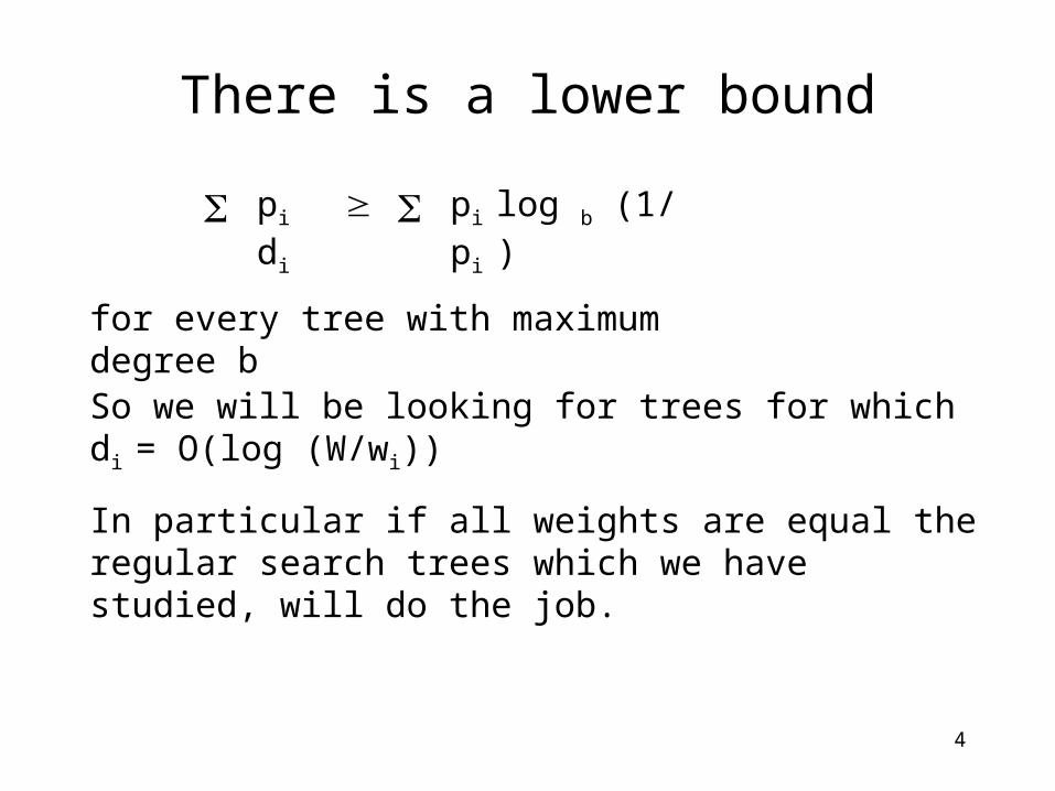
There is a lower bound
So we will be looking for trees for which di = O(log (W/wi))
pi di pi log b (1/ pi )
for every tree with maximum degree b
In particular if all weights are equal the regular search trees which we have studied, will do the job.
5
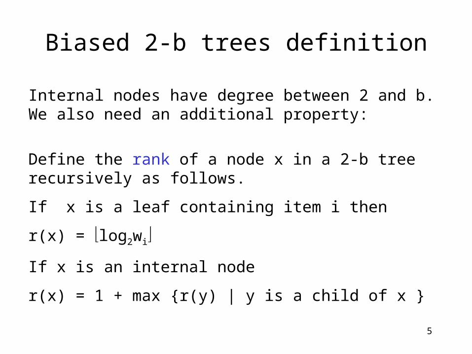
Biased 2-b trees definition
Internal nodes have degree between 2 and b. We also need an additional property:
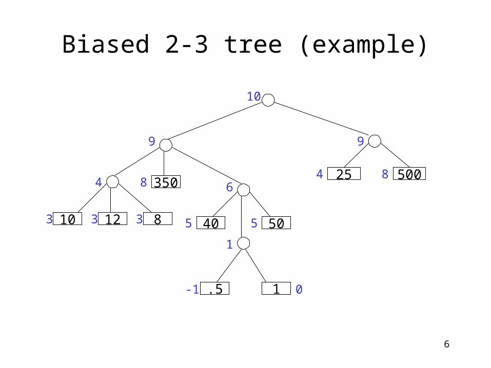
Define the rank of a node x in a 2-b tree recursively as follows.
If x is a leaf containing item i then
r(x) = log2wi
If x is an internal node
r(x) = 1 + max {r(y) | y is a child of x }
6
Biased 2-3 tree (example)
35050025
10 12 8 40 50
.5 1
84
9
10
0-1
55
1
68
333
4
9
7
Biased 2-b trees definition (cont)
Call x major if r(x) = r(p(x)) - 1
Otherwise x is minor
Local bias: Any neighboring sibling of a minor node is a major leaf.
In case all weights are the same this implies that all leaves should be at the same level and we get regular 2-b trees.
Here is the additional property:
8
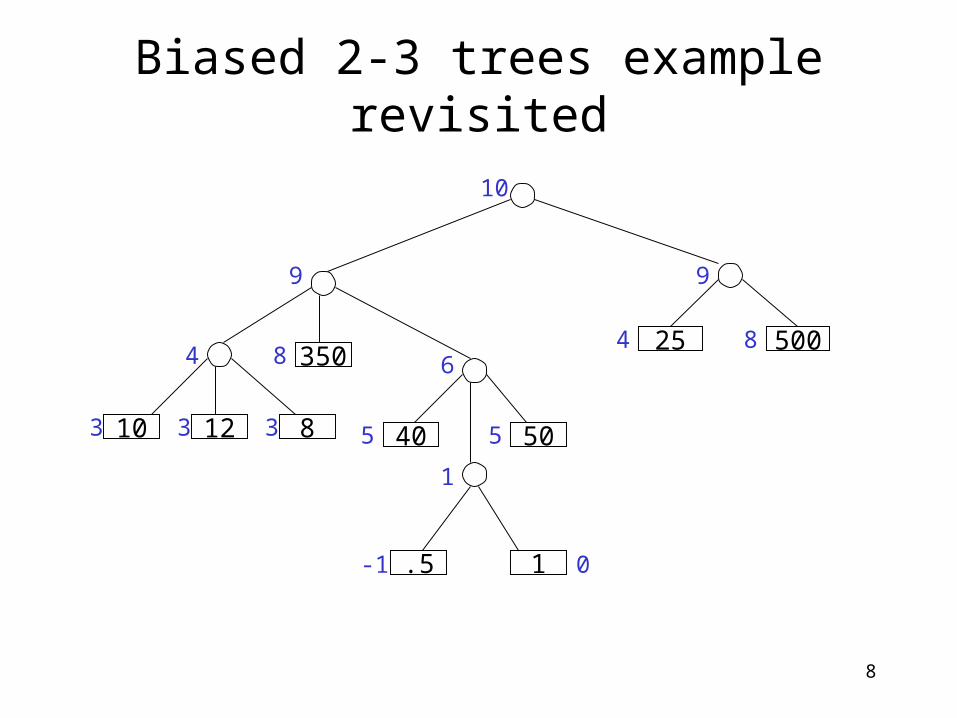
Biased 2-3 trees example revisited
35050025
10 12 8 40 50
.5 1
84
9
10
0-1
55
1
68
333
4
9

9
Are the access times ok ?Define the size of a node x in a 2-b tree recursively as follows.
If x is a leaf containing item i s(x) = wi
If x is an internal node s(x) = y is a child of x s(y)
Lemma: For any node x, 2r(x)-1 s(x),
For a leaf x, 2r(x) s(x) < 2r(x) +1
==> if x is a leaf of depth d then d < log(W/ wi) + 2
proof. D r(root) - r(x) < log (s(r)) + 1 - (log(s(x)) - 1)
10
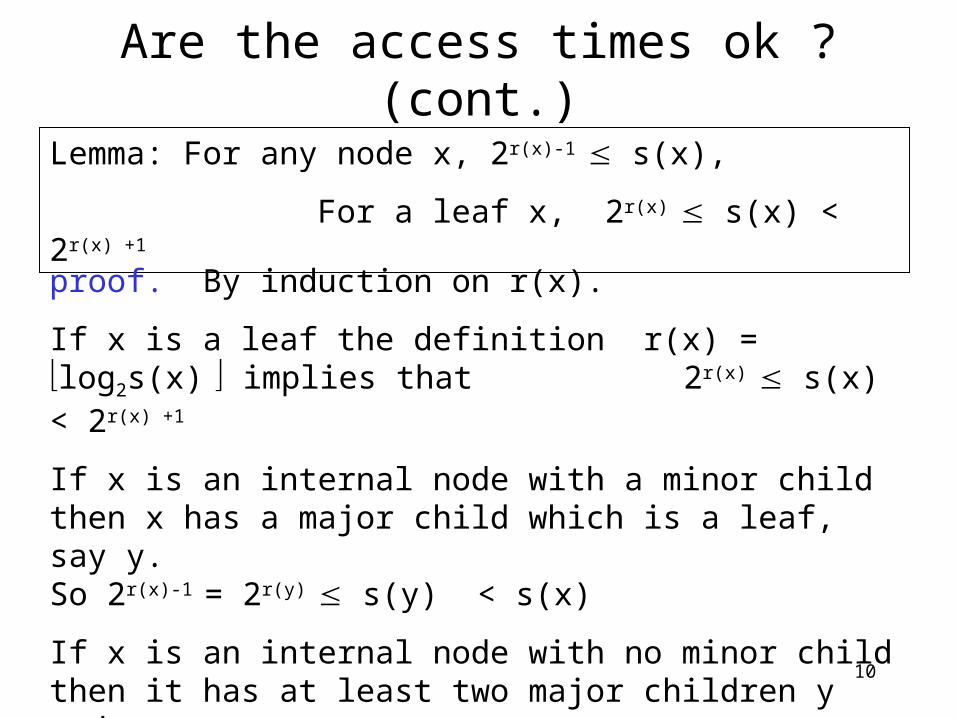
Are the access times ok ? (cont.)
Lemma: For any node x, 2r(x)-1 s(x),
For a leaf x, 2r(x) s(x) < 2r(x) +1
proof. By induction on r(x).
If x is a leaf the definition r(x) = log2s(x) implies that 2r(x)
s(x) < 2r(x) +1
If x is an internal node with a minor child then x has a major child which is a leaf, say y. So 2r(x)-1 = 2r(y) s(y) < s(x)
If x is an internal node with no minor child then it has at least two major children y and z:
2r(x)-1 = 2r(y)-1 + 2s(z)-1 s(y) + s(z) s(x)

11
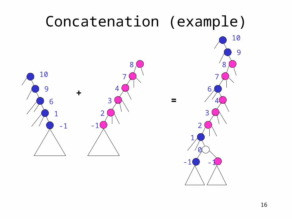
Concatenation (example)
9
108
6
1
-1
7
4
3
2
-1
+
9
10
8
6
1
-1
7
4
3
2
-1
0
=
12
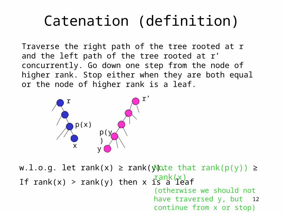
Catenation (definition)
Traverse the right path of the tree rooted at r and the left path of the tree rooted at r’ concurrently. Go down one step from the node of higher rank. Stop either when they are both equal or the node of higher rank is a leaf.
yx
w.l.o.g. let rank(x) ≥ rank(y).
If rank(x) > rank(y) then x is a leaf
p(x)p(y)
Note that rank(p(y)) ≥ rank(x)
(otherwise we should not have traversed y, but continue from x or stop)
r r’
13
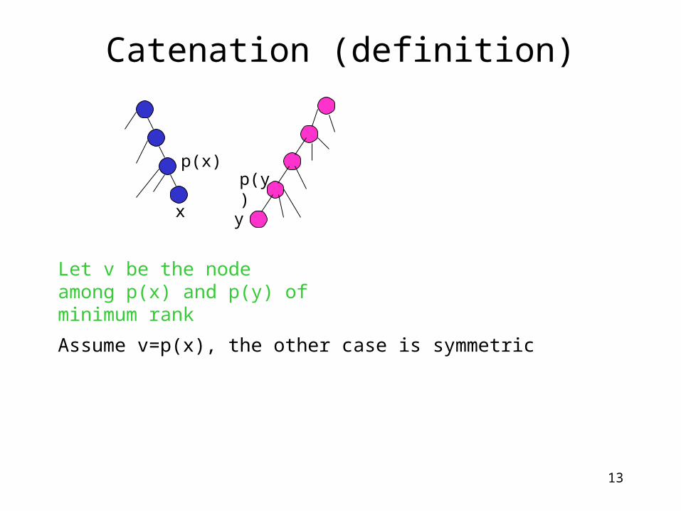
Catenation (definition)
Assume v=p(x), the other case is symmetric
yx
p(x)p(y)
Let v be the node among p(x) and p(y) of minimum rank
14
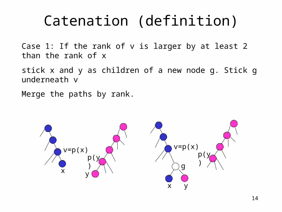
Catenation (definition)
Case 1: If the rank of v is larger by at least 2 than the rank of x
stick x and y as children of a new node g. Stick g underneath v
Merge the paths by rank.
yx
v=p(x)p(y)
yx
v=p(x)p(y)
g
15
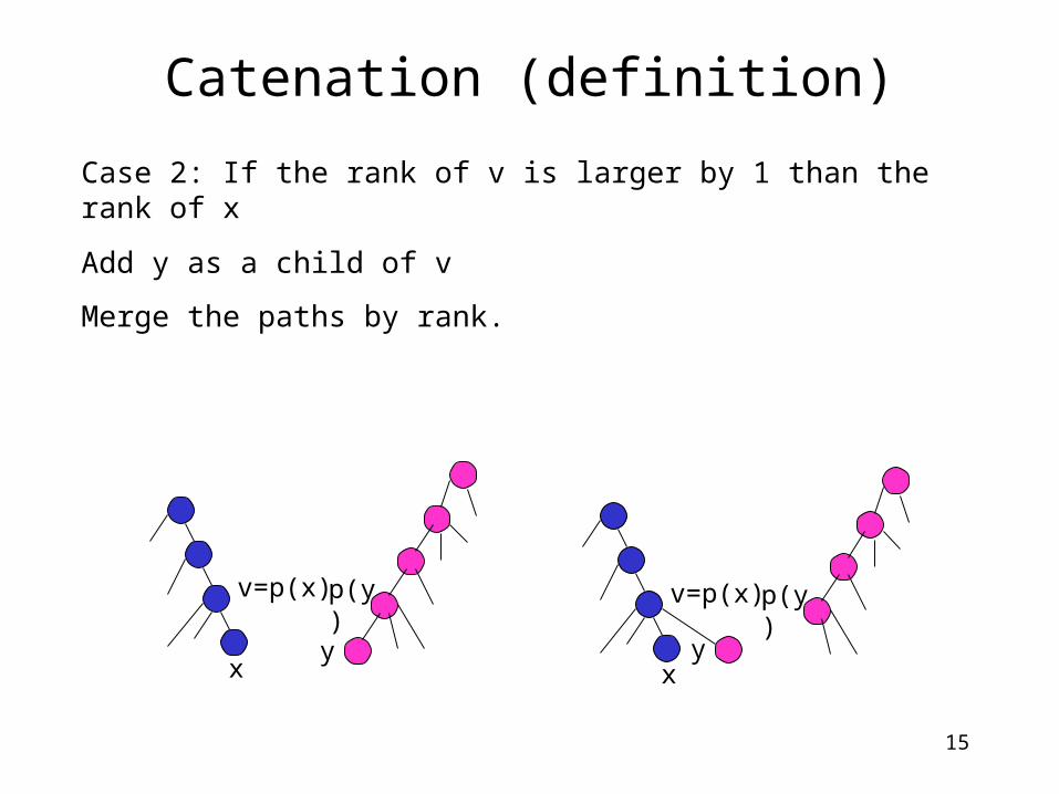
Catenation (definition)
Case 2: If the rank of v is larger by 1 than the rank of x
Add y as a child of v
Merge the paths by rank.
yx
v=p(x) p(y)
yx
v=p(x) p(y)
16
Concatenation (example)
9
108
6
1
-1
7
4
3
2
-1
+
9
10
8
6
1
-1
7
4
3
2
-1
0
=
17
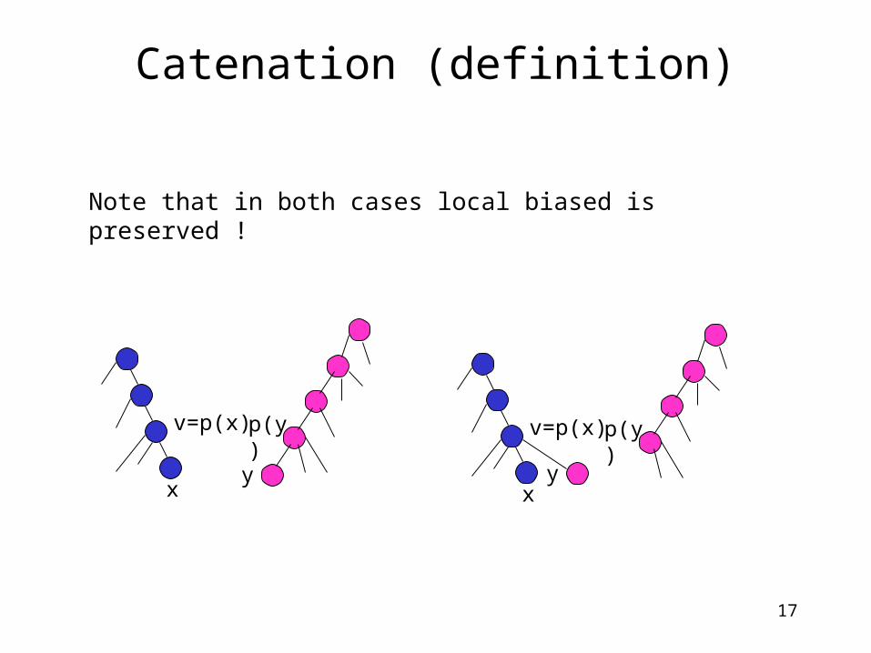
Catenation (definition)
Note that in both cases local biased is preserved !
yx
v=p(x) p(y)
yx
v=p(x) p(y)
18
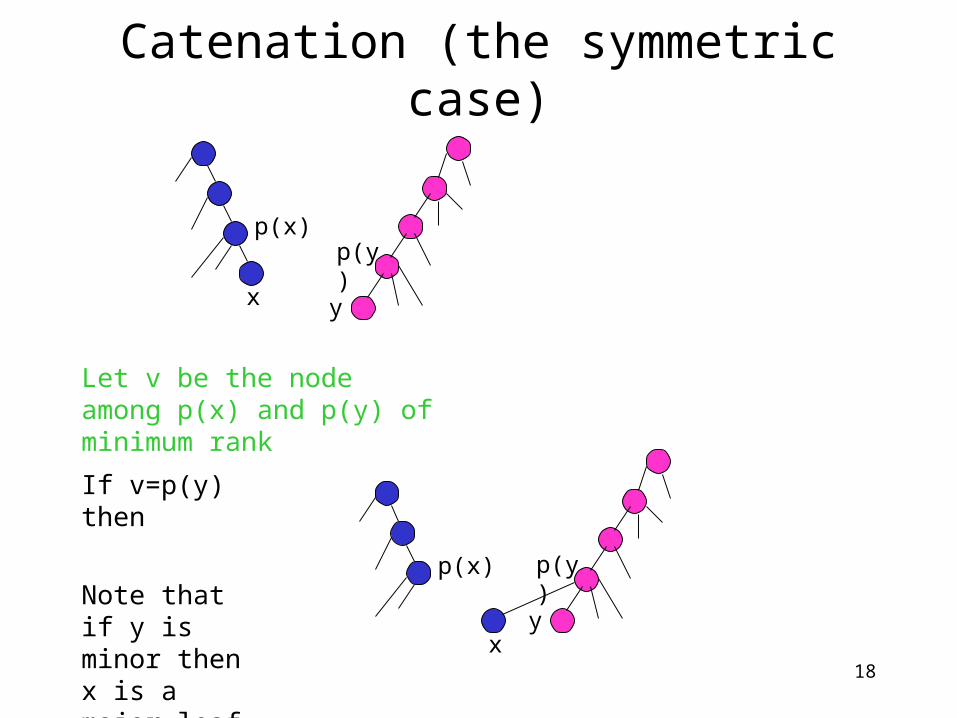
Catenation (the symmetric case)
If v=p(y) then
yx
p(x)p(y)
Let v be the node among p(x) and p(y) of minimum rank
yx
p(x) p(y)Note that if y is minor then x is a major leaf
21
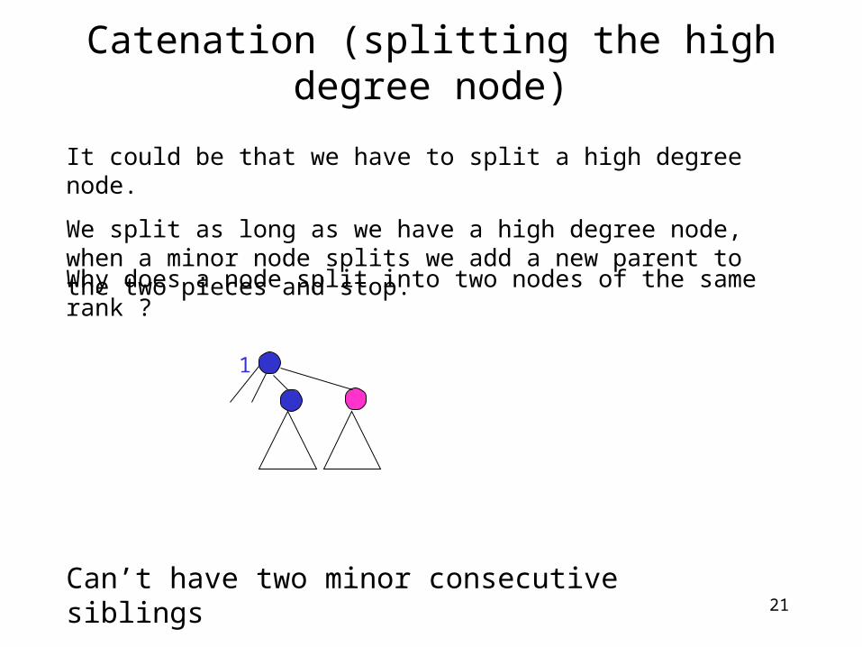
Catenation (splitting the high degree node)
Why does a node split into two nodes of the same rank ?
1
Can’t have two minor consecutive siblings
It could be that we have to split a high degree node.
We split as long as we have a high degree node, when a minor node splits we add a new parent to the two pieces and stop.
22
Catenation (proof of correctness)
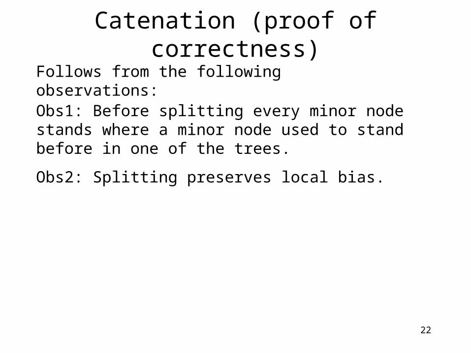
Obs1: Before splitting every minor node stands where a minor node used to stand before in one of the trees.
Obs2: Splitting preserves local bias.
Follows from the following observations:
23
Catenation (worst case analysis)
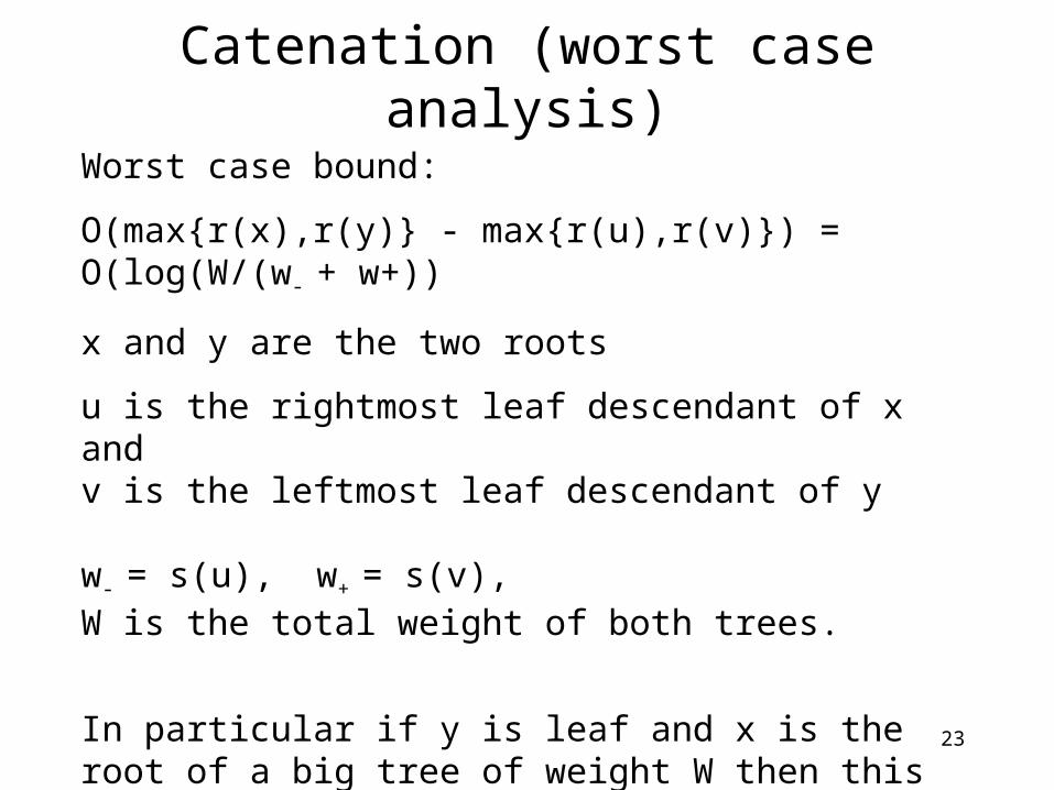
Worst case bound:
O(max{r(x),r(y)} - max{r(u),r(v)}) = O(log(W/(w- + w+))
x and y are the two roots
u is the rightmost leaf descendant of x andv is the leftmost leaf descendant of y
w- = s(u), w+ = s(v), W is the total weight of both trees.
In particular if y is leaf and x is the root of a big tree of weight W then this bound is O(W/s(y))
24
Catenation (amortized analysis)
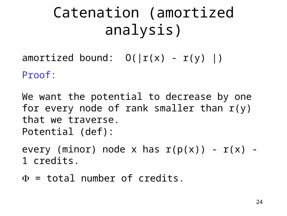
amortized bound: O(|r(x) - r(y) |)
Potential (def):
every (minor) node x has r(p(x)) - r(x) - 1 credits.
= total number of credits.
We want the potential to decrease by one for every node of rank smaller than r(y) that we traverse.
Proof:
25
Catenation (amortized analysis)
a
a
b
cd
e
bc
de
f
+
a
ab
c
d
e
b
cd
e
f
=
26
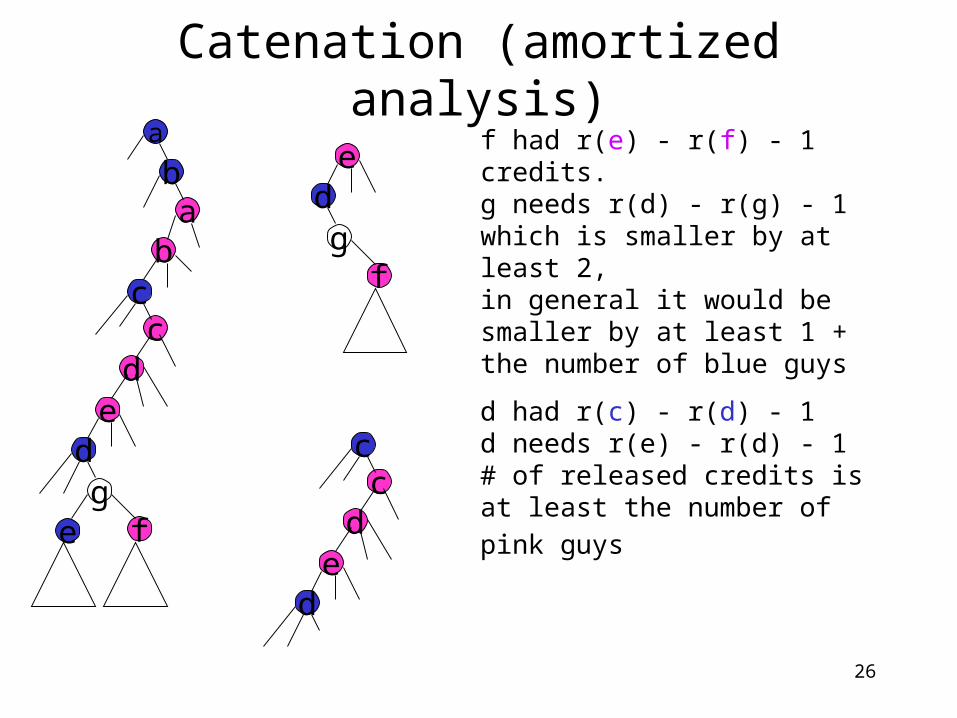
Catenation (amortized analysis)a
ab
c
d
e
b
cd
e
fg
de
fg
f had r(e) - r(f) - 1 credits.g needs r(d) - r(g) - 1which is smaller by at least 2,in general it would be smaller by at least 1 + the number of blue guys
c
d
cd
e
d had r(c) - r(d) - 1d needs r(e) - r(d) - 1# of released credits is at least the
number of pink guys
27
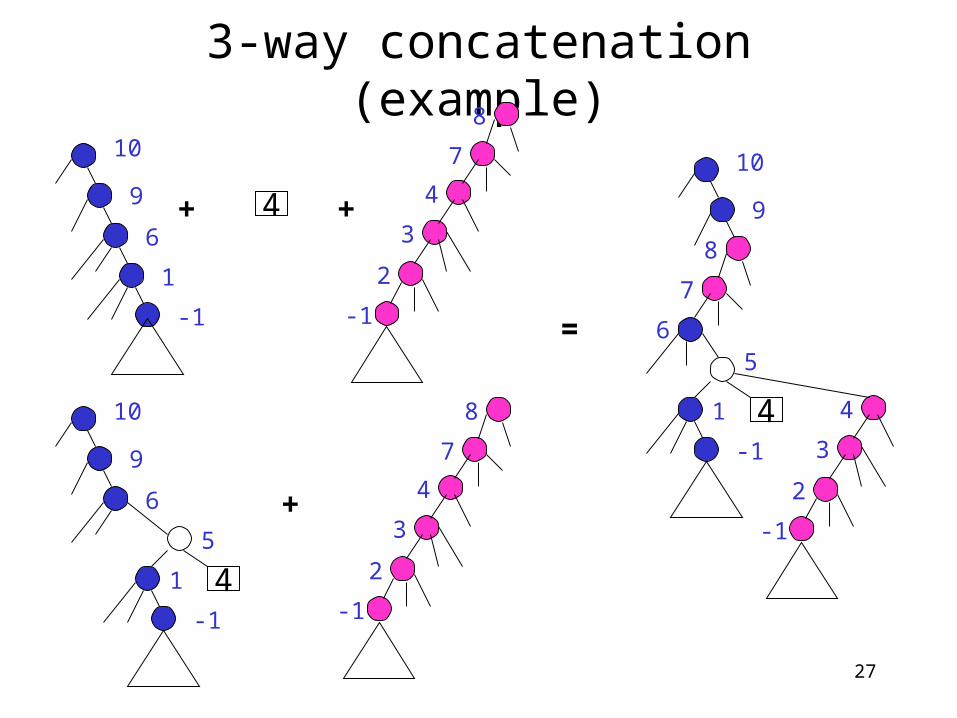
3-way concatenation (example)
9
108
6
1
-1
7
4
3
2
-1
+
=
+ 4
9
10
6
1
-1
+
4
8
7
4
3
2
-1
5
9
10
8
6
7
1
-1
4 4
3
2
-1
5
28
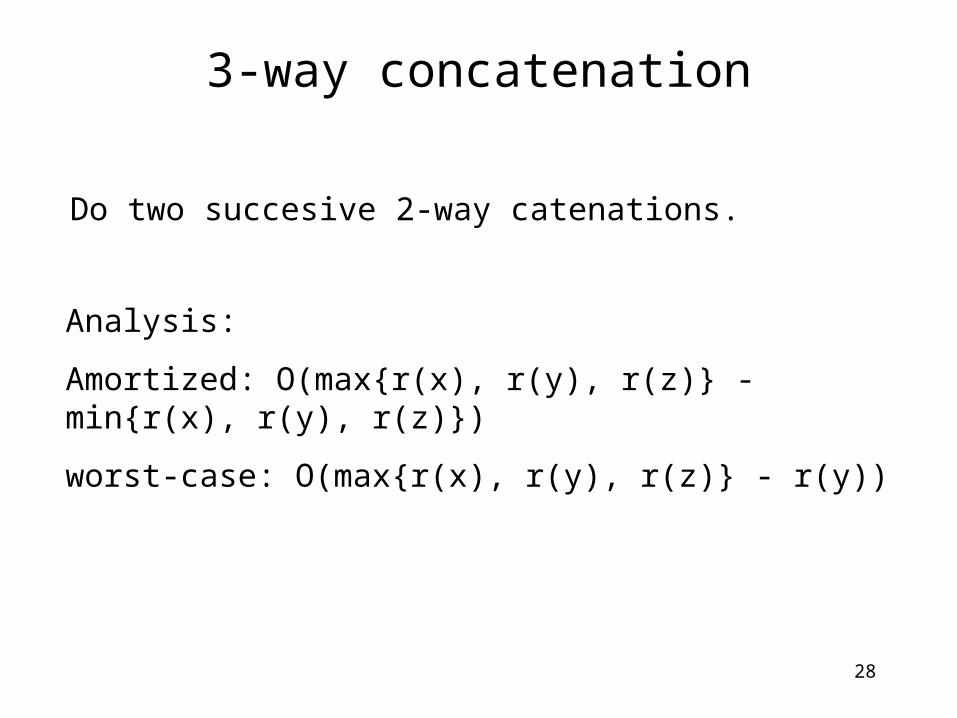
3-way concatenation
Do two succesive 2-way catenations.
Analysis:
Amortized: O(max{r(x), r(y), r(z)} - min{r(x), r(y), r(z)})
worst-case: O(max{r(x), r(y), r(z)} - r(y))
29
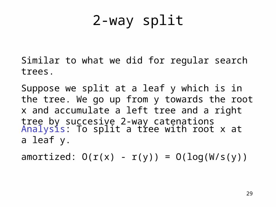
2-way split
Similar to what we did for regular search trees.
Suppose we split at a leaf y which is in the tree. We go up from y towards the root x and accumulate a left tree and a right tree by succesive 2-way catenations
Analysis: To split a tree with root x at a leaf y.
amortized: O(r(x) - r(y)) = O(log(W/s(y))
30
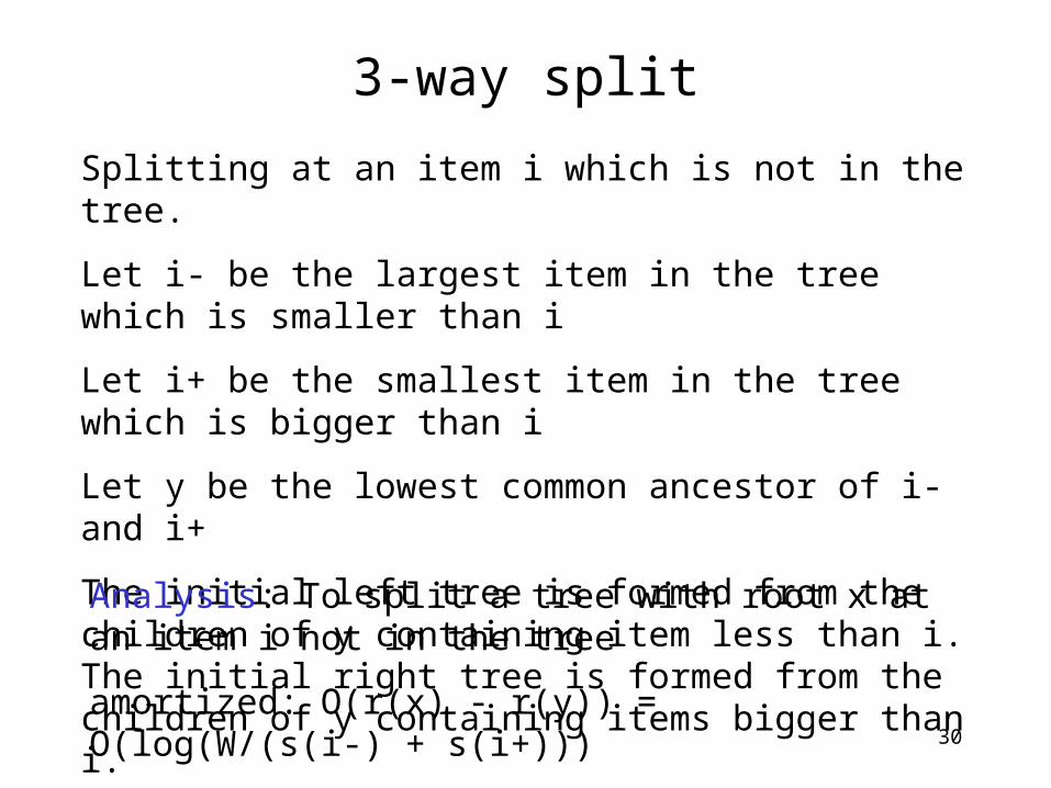
3-way split
Splitting at an item i which is not in the tree.
Let i- be the largest item in the tree which is smaller than i
Let i+ be the smallest item in the tree which is bigger than i
Let y be the lowest common ancestor of i- and i+
The initial left tree is formed from the children of y containing item less than i. The initial right tree is formed from the children of y containing items bigger than i.
Analysis: To split a tree with root x at an item i not in the tree
amortized: O(r(x) - r(y)) = O(log(W/(s(i-) + s(i+)))
31
Other operations
Define delete, insert, and weight change in a straightforward way in terms of catenate and split.
32
Extensions
There are many variants.
Binary variants.
Variants that has good bounds for all operations on the worst case
![eprojekt.hreprojekt.hr/Brosura.pdf · w } i l t µ À o i v i } i l ] u ï l ñ ì ^ z : ^ z : x x x x x x x x x x x x x x x x x x x x x x x x x x x x x x x x x x x x x x x x x x](https://img.pdfslide.net/doc/110x75/5dd13499d6be591ccb64ba3d/w-i-l-t-o-i-v-i-i-l-u-l-z-z-x-x-x-x-x-x-x-x-x-x-x-x.jpg)


![k|x/L lgodfjnL, @)&! · -6_ æk|x/L cltl/Qm cfo'QmÆ eGgfn] dxfgu/Lo k|x/L cGtu{t sfo{/t k|x/L gfoj dxflg/LIfs ;Demg' k5{ . -7_ æk|x/L cfo'QmÆ eGgfn] dxfgu/Lo k|x/L sfof{nosf] k|d'v](https://img.pdfslide.net/doc/110x75/6077828ea38c8056df0a6097/kxl-lgodfjnl-6-kxl-cltlqm-cfoqm-eggfn-dxfgulo-kxl-cgtut.jpg)
![5. Nastavna cjelina - Ekonomski odnosi s …^ À µ ] o ] : X : X ^ } u Ç µ K ] i l µ U l } v } u l ] ( l µ o µ K ] i l µ U ] Ì À X } ( X X X E À v l U ' } } À } , À l r](https://img.pdfslide.net/doc/110x75/5e236f8c507ff210b41e0a8c/5-nastavna-cjelina-ekonomski-odnosi-s-o-x-x-u-k-i.jpg)


![]L]E X l° a K ^è] S X L](https://img.pdfslide.net/doc/110x75/5a7e22e97f8b9a66798e369f/le-x-l-a-k-s-x-lc-c-c-epzj-sw-.jpg)