Embed Size (px)
Citation preview

1
Bunched-Beam Envelope Simulation with Space Charge within the SAD
Environment
Christopher K. AllenLos Alamos National Laboratory

Dec, 2005 C.K. Allen
2
Abstract
The capability for simulating the envelopes of three-dimensional (bunched) beams has been implemented in the SAD accelerator modeling environment. The simulation technique itself is similar to that of other common envelope codes, such as Trace3D, TRANSPORT, and the XAL online model. Specifically, we follow the second-order statistics of the beam distribution rather than tracking individual particles. If we assume that the beam maintains ellipsoidal symmetry in phase space, we can include the first order effects due to space charge using a semi-analytic model. This is the attractive characteristic of envelope codes, since it greatly reduces computational time. This new feature of SAD is implemented primarily in the SADScript interpreted language, with only a small portion appearing as compiled code. As such, the simulation does run slower than other compiled envelope codes such as TRACE3D or XAL, however, as interpreted code it does have the benefit of being easily modified. We demonstrate use of the new feature and present example simulations of the J-PARC linear accelerator section.

Dec, 2005 C.K. Allen
3
Outline1. Overview
1. Motivation2. Basic Approach
2. Envelope Dynamics Review
3. SADScript Implementation
4. (Field Calculations)
5. Simulation Results
6. Issues and Conclusions

Dec, 2005 C.K. Allen
4
1. Overview
Motivation
To have envelope simulation capability for three-dimensional (bunched) beams, including space-charge, within the SAD environment.
Such an engine is useful for\ Model reference (Fast) Low energy electron simulation Proton simulation Longitudinal effects

Dec, 2005 C.K. Allen
5
1. Overview (cont.)
RMS Envelope – Approach Used Within SAD Environment
The simulation principle is that same as that used by Trace3D and TRANSPORT. Specifically, it is an extension of linear beam optics to the second-order moment dynamics.
For a beam optics model we require a matrix sc to account for the linear part of the space-charge force, it is accurate only over short distances s.
In the SAD environment we are given the full transfer matrix n for each element n. We must take the Nth root of each n where N = Ln/s is the number of space charge “kicks” to be applied within the element.
The space charge matrix sc depends upon the second moments, however, by the dynamics equations the second moments depend upon sc. Thus, we have self-consistency issues and must employ a propagation algorithm that maintains a certain level of consistency.

Dec, 2005 C.K. Allen
6
2. Envelope Dynamics Review
RMS envelope simulation is based on the following: Phase space coordinates z = (x x’ y y’ z dp)T
Linear beam optics - transfer matrices zn+1 = n zn
Moment operator , g g(z)f(z)d6z
Moment matrix = zzT
Propagation of moment matrix n+1 = nnnT
Dec, 2005 C.K. Allen
7
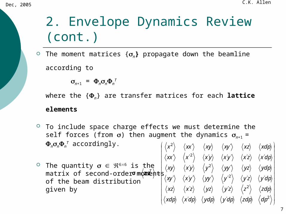
2. Envelope Dynamics Review (cont.) The moment matrices {n} propagate down the beamline according to
n+1 = nnnT
where the {n} are transfer matrices for each lattice elements
To include space charge effects we must determine the self forces (from ) then augment the dynamics n+1 = nnn
T accordingly.
The quantity 66 is the matrix of second-order moments of the beam distribution given by
2
2
2
2
2
2
dpzdpdpyydpdpxxdp
zdpzzyyzzxxz
dpyzyyyyyxyx
ydpyzyyyyxxy
dpxzxyxyxxxx
xdpxzyxxyxxx
Tzzσ

Dec, 2005 C.K. Allen
8
3. SADScript ImplementationOverview
Register the beamline with the SAD environment using GetMAIN[latticeFile] where latticeFile is the input deck describing the machine
Acquire the set of transfer matrices {n} and lengths {Ln} for all beamline elements from the SAD environment
Take the Nth root of each transfer matrix where N is the number of space charge “kicks” to be applied within the element. This is done using the matrix logarithm function.
Propagate moment matrix through each element using above transfer matrix and the space charge matrix sc computed for each step s
Dec, 2005 C.K. Allen
9
3. SADScript Implementation (cont.)Initialization
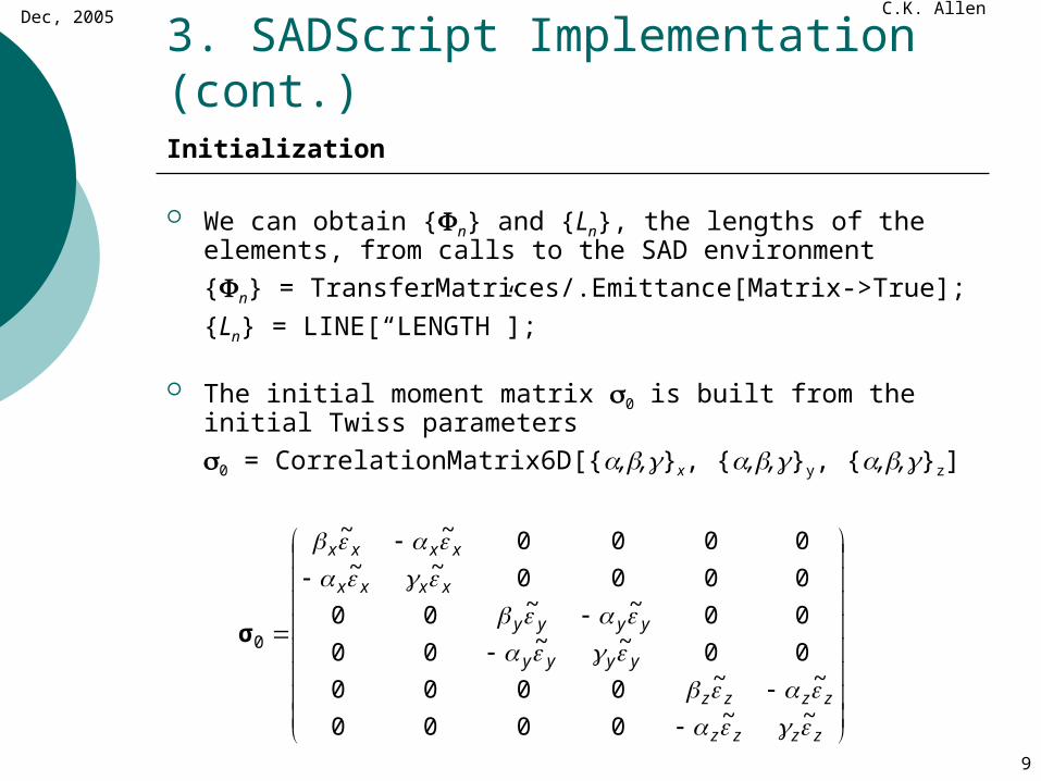
We can obtain {n} and {Ln}, the lengths of the elements, from calls to the SAD environment
{n} = TransferMatrices/.Emittance[Matrix->True];
{Ln} = LINE[“LENGTH”];
The initial moment matrix 0 is built from the initial Twiss parameters
0 = CorrelationMatrix6D[{,,}x, {,,}y, {,,}z]
zzzz
zzzz
yyyy
yyyy
xxxx
xxxx
~~0000
~~0000
00~~00
00~~00
0000~~0000~~
0σ

Dec, 2005 C.K. Allen
10
3. SADScript Implementation (cont.)Sub-Dividing Beamline Elements (the Nth root of n)
The transfer matrix n for an element n has the form
n = exp(LnFn)
where Ln is the length of the element and Fn is the generator matrix which represents the external forces of element n.
To sub-divide element n, we require the matrix Fn, given by
Fn = log(n)/Ln
The “sub-transfer matrix” n(s) for element n can then be computed as
n(s)= exp(sFn)

Dec, 2005 C.K. Allen
11
3. SADScript Implementation (cont.)Transfer Matrices with Space Charge Whether using the equations of motion or Hamiltonian formalism, within
a section s of a element n we can write the first-order continuous dynamics as
z’(s) = Fnz(s) + Fsc()z(s)
where the matrix Fn represents the external force of element n and Fsc() is the matrix of space charge forces.
For Fsc() constant, the solution is z(s) = exp[s(Fn + Fsc)]z0.
Thus, the full transfer matrix including space charge should be
n = exp[s(Fn+Fsc)]

Dec, 2005 C.K. Allen
12
3. SADScript Implementation (cont.)Numerical Efficiency For a step size of s, rather than computing the “exact” transfer matrix
n(s) = exp[s(Fn+Fsc)],
we compute a transfer matrix which is second-order accurate in s.
Note that
n(s) = sc(s/2) n(s) sc(s/2) + O(s3)
where n(s) = exp(sFn) (computed once per element)
sc(s/2) = exp(s/2Fsc) = I + s/2Fsc (by idempotency, Fsc2 = 0)
We have reduced a matrix exponentiation at each step s to one matrix addition and two matrix multiplications
Dec, 2005 C.K. Allen
13
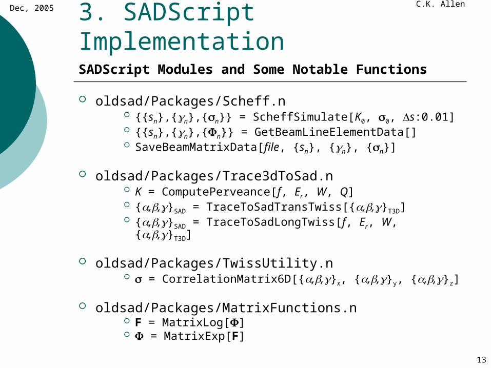
3. SADScript ImplementationSADScript Modules and Some Notable Functions
oldsad/Packages/Scheff.n {{sn},{n},{n}} = ScheffSimulate[K0, 0, s:0.01] {{sn},{n},{n}} = GetBeamLineElementData[] SaveBeamMatrixData[file, {sn}, {n}, {n}]
oldsad/Packages/Trace3dToSad.n K = ComputePerveance[f, Er, W, Q] {,,}SAD = TraceToSadTransTwiss[{,,}T3D] {,,}SAD = TraceToSadLongTwiss[f, Er, W, {,,}T3D]
oldsad/Packages/TwissUtility.n = CorrelationMatrix6D[{,,}x, {,,}y, {,,}z]
oldsad/Packages/MatrixFunctions.n F = MatrixLog[] = MatrixExp[F]

Dec, 2005 C.K. Allen
14
4. Field Calculations
Space charge effects are included by assuming the beam has ellipsoidal symmetry with dimensions corresponding to the statistics in .
f(z) = f(zT1z)
Analytic field expressions for such a bunch distributions are available
where a, b, c, are the semi-axes of the ellipsoid (depends upon ) and (x,y,z) are the coordinates along the semi-axes
02/122/122/12
0
2
2
2
2
2
2 )()()(
)(
4),,(
ct
z
bt
y
at
x
dsdtctbtat
sfqabczyx
ab
c
x
y
z

Dec, 2005 C.K. Allen
15
4. Field Calculations (cont.)Coordinate Transformations To apply the previous formula for we must rotate to the coordinates of
the beam ellipsoid semi-axes using a transformation
R SO(3) SO(6).
Moreover, we require a transformation G = diag(1,1,1,1,,1/) to convert longitudinal coordinates from (z,dp) to (z,z’) (momentum to primed)
The complete transformation is
= RTGTGR
where the xy, xz, yz elements of are zeroIt is important that this transform is numerically accurate!

Dec, 2005 C.K. Allen
16
4. Field Calculations (cont.)Take the Linear Part of the Electric Fields
To each electric self-field component Ex, Ey, Ez is expanded in the form
Ex = a1x + a2y + a3z (e.g., for x plane)
Multiplying the above equation by the functions {x,y,z} then taking moments
if xy = xz = yz (transform GR) we have
This is the weighted, least-squares, linear approximation for the self fields
x
x
x
zE
yE
xE
a
a
a
zyzxz
yzyxy
xzxyx
3
2
1
2
2
2
xx
xEzyxE x
x 2),,(

4. Field Calculations (cont.)Field Moments
For ellipsoidal beams having a density distribution f, the self-field moments can be calculated from and are given by the following:
ab
c
x
y
z
where (f) is almost constant (F. Sacherer) and RD is the elliptic integral
0 2/32/12/12
3),,(
ztytxt
dtzyxRD
,,,
243
)(
,,,243
)(
,,,243
)(
2222
0
2222
0
2222
0
zyxRzQf
zE
yxzRyQf
yE
xzyRxQf
xE
Dz
Dy
Dx

Dec, 2005 C.K. Allen
18
4. Field Calculations (cont.)Space Charge Generator Matrix
Thus, the full space charge generator matrix Fsc() is given by
where
11
0/10000
000000
000/100
000000
00000/1
000000
)(
GRRGσF T
z
y
x
sc
f
f
f
2222/3
2
2222/3
2222/3
,,52
1
,,52
1
,,52
1
zyxRK
f
yxzRK
f
xzyRK
f
Dz
Dy
Dx

5. Simulation Results
J-PARC BT Line Simulation Show SADScript envelope
simulation of the J-PARC BT line for several cases
Zero current 30 mA 130 mA
Compare the SADScript envelope simulation to simulations provided by Trace3D Notable differences
Trace3D does not impose symplectic condition
Trace3D can simulate emittance growth thru RF Gaps (removed)

5. J-PARC Simulation0 mA
0
10
20
30
0 40 80 120 160 200
s (m)
rad/m T3D
SAD
0
10
20
30
0 40 80 120 160 200
s (m)
rad/m T3D
SAD
0
300
600
900
1200
0 40 80 120 160 200
s (m)
rad/m T3D
SAD
Horizontal x(s) Vertical y(s)
Longitudinal z(s)
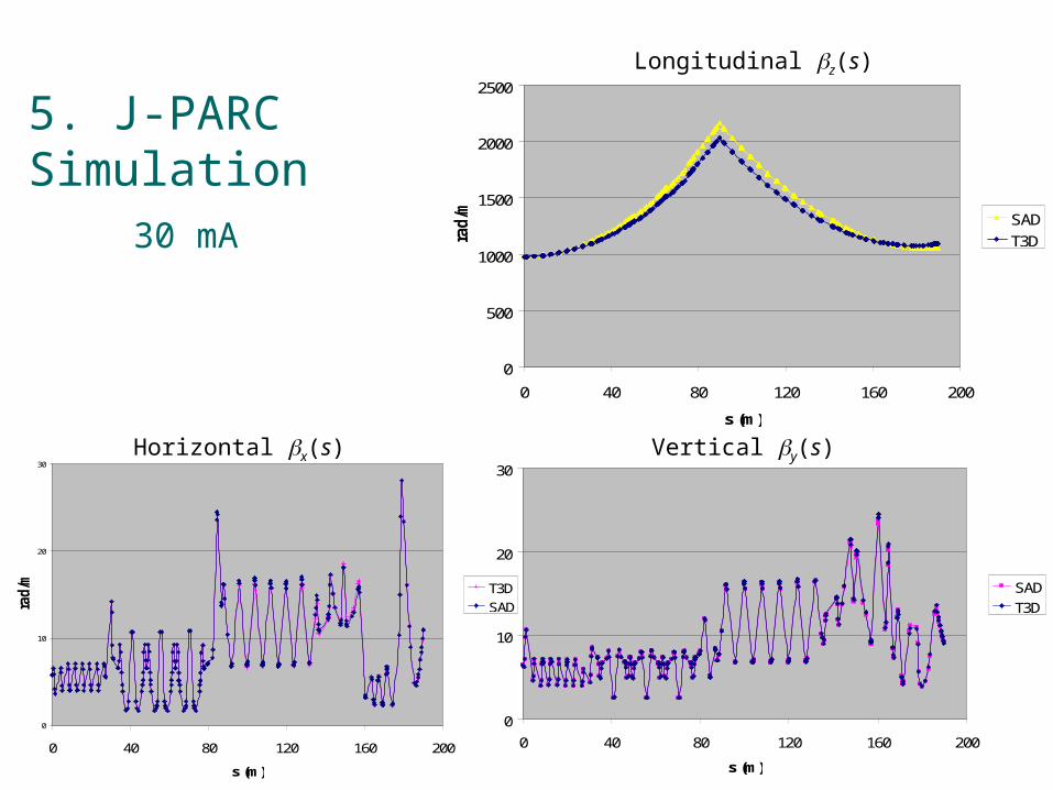
5. J-PARC Simulation30 mA
0
10
20
30
0 40 80 120 160 200
s (m)
rad/m T3D
SAD
0
10
20
30
0 40 80 120 160 200
s (m)
SAD
T3D
Horizontal x(s) Vertical y(s)
Longitudinal z(s)
0
500
1000
1500
2000
2500
0 40 80 120 160 200
s (m)
rad/m SAD
T3D

5. J-PARC Simulation130 mA
0
10
20
30
40
0 40 80 120 160 200
s (m)
rad/m SAD
T3D
0
10
20
30
40
0 40 80 120 160 200
s (m)
SADT3D
Horizontal x(s) Vertical y(s)
Longitudinal z(s)
0
2000
4000
6000
8000
0 40 80 120 160 200
s (m)
rad/m SAD
T3D

Dec, 2005 C.K. Allen
23
6. Issues
Computation of the matrix logarithm log(n) is expensive. Current procedure uses an iterative technique which
computes a matrix exponential exp(Fn) at each step
The procedure works for n close to the identity matrix I It is not robust, but it should suffice for symplectic
matrices
Computation of the matrix exponential exp(Fn) is also non-trivial Use a Taylor expansion with scaling and squaring.

Dec, 2005 C.K. Allen
24
6. Issues (cont.)
Currently only a simple stepping procedure is employed. The step size s remains constant throughout simulation By implementing an adaptive stepping algorithm we can obtain
significant speedup and maintain a specified level of accuracy in the solution (see “Bunched Beam Envelope Simulation with Space Charge”, KEK, Jan 20, 2005.)
The longitudinal space charge force seems to be slightly stronger in all SAD simulations as compared to Trace3D. I have debugged the SAD code extensively and have not found
any errors in the theory or implementation. I believe this condition is simply a result of the difference in
simulation architecture, but I may be wrong.

Dec, 2005 C.K. Allen
25
6. Conclusions A major issue is computational speed
For the J-PARC simulation Trace3D runs on the order of 0.5 seconds SAD ScheffSimulate runs on the order of 0.5 minutes
By implementing the adaptive stepping and/or implementing the computationally expensive functions as compiled code we should see significant speedup. Only the elliptic integral function RD(x,y,z) in implemented in
compiled code. Implementing MatrixExp() as compile code would be the most
cost-effective
The small difference in longitudinal dynamics between SAD and Trace3D may be an artifact of the different approaches. However, I am not sure.

Dec, 2005 C.K. Allen
26
3. SADScript Implementation Initialization
Load the beamline information from the target “input deck” We acquire all the transfer matrices {n} and all the element
lengths {Ln}
Space Charge Compute the partial transfer matrix n(s) where s = Ln/N Compute space charge transfer matrix sc for a distance s. Combine n (s) and sc for full transfer matrix n,sc(s)
Propagation Propagate n through element using i+1 = n,sc(s)in,sc(s)T
recomputing n,sc(s) as necessary Propagate {n} through beamline using above procedure for each
element n.

Dec, 2005 C.K. Allen
27
3. SADScript Implementation (cont.)Beam Dynamics with Space ChargeTo include space charge effects we must determine the self forces then augment
the dynamics n+1 = nnnT to include them.
To propagate the moment matrix n through an element we must compute a transfer matrix n,sc that includes space charge. Such a transfer matrix can only be computed accurately for a short distance s < Ln We must divide each beamline element into sub-elements of length s having the
appropriate transfer matrix Nn We apply the dynamics n+1 = Nnn
NnT many times, recomputing
We use a “kick-like” approach - correcting the beam state at regular intervals through each element
We divide each beamline element into sub-elements of length s
We represent the self force through s as a transfer matrix sc
Because the self forces depend upon the beam shape, the matrix self force transfer matrix sc depends upon the moment matrix


![Retroflex versus bunched [r] in compensation for ...linguistics.berkeley.edu/phonlab/documents/2011/retrobunch_paper.pdf · Retroflex versus bunched [r] in compensation for coarticulation](https://img.pdfslide.net/doc/110x75/5b09bbee7f8b9a992a8e2cb3/retroflex-versus-bunched-r-in-compensation-for-versus-bunched-r-in-compensation.jpg)