Hierarchical Organization ofModularity in Metabolic Networks

Supporting Online Material

Contents

1 Network Models 2

2 Graph Theoretic Representation of the Metabolic Network 9

3 Clustering and Functional Characterization 16

1

1. Network Models

1.1 Scale-free and Modular Networks

1.1.1 Models

The scale-free model (Fig. 1a, article)

The scale-free model is generated from a small initial core of connected nodes withthe addition of a new node in each timestep[1]. This new incoming node connects mundirected and unweighted links to the existing nodes following preferential attachment.The probability Πi of the new node to attach to node i is proportional to the numberof links node i already has:

Πi =ki∑ki

.

The modular model (Fig. 1b, article)

The modular model is a generalization of the Erdos-Renyi random graph[2]. Insteadof starting with N nodes and connecting all nodes with probability p, we start with mgroups of nodes of relative sizes f1, f2, . . ., fm (

∑fi = 1). We connect all nodes within

a group (module) with probability q and connect all pairs belonging to different groupswith probability p << q. This model gives rise to a random, but inherently modularnetwork. A closely related model was proposed recently in Ref [3].

1.1.2 Properties of the model networks

Degree distribution

The degree distribution is defined as the probability P (k) that a randomly chosen nodein the network has a degree (number of links) k.

• For the scale-free model P (k) ∼ k−3 (Fig. S1a)[1]. Such power-law dependencemeans that there is no characteristic scale for the degree values; while an averageconnectivity can be defined, the second momentum of the distribution diverges.

2

• For a random network the degrees follow a Poisson distribution, characterized byan exponential tail. The average connectivity for such a graph has well-definedaverage value, and the second moment of the distribution is finite. The degreedistribution of the modular network model (Fig. 1b, article) has an exponentialtail, the modularity having little affect on degree distribution. Thus its degreedistribution is similar to that of a random graph (Fig. S1b).

1 10 100 1000k

10−6

10−5

10−4

10−3

10−2

10−1

100

P(k

)

N=2*10^5N=2*10^4N=2*10^3N=2*10^2

(a) Scale-free networks.

0 10 20 30k

10−6

10−4

10−2

100

P(k

)

0 10 20 30k

0

0.05

0.1

0.15

0.2

P(k

)

N=2*10^5N=2*10^4N=2*10^3N=2*10^2

(b) Modular networks.

Figure S1. Degree distributions of model networks with different sizes (< k > = 6).

Clustering coefficient

The clustering coefficient of a node gives the probability that its neighbors are connectedto each other. It is defined as[4]

Ci =2n

ki (ki − 1),

where n denotes the number of direct links connecting the ki nearest neighbors of nodei. The clustering coefficient is close to one for a node at the center of a highly interlinkedcluster, while it is zero for a node that is part of an only loosely connected group. There-fore Ci, averaged over all nodes i, is a measure of the network’s potential modularity,since it offers a measure of the degree of interconnectivity in the neighborhood of eachnode. For example, a node whose neighbors are all connected to each other has C = 1(Fig. S2, left), while one with no links between its neighbors has C = 0 (Fig. S2, right).A network for which the average clustering coefficient is large is expected to be highlyinterconnected, a sign of clustering.

The average clustering coefficient of the scale-free model generated for different net-work sizes is known to decrease as N−3/4 (See Fig. 2b from article).

3

C=1 C=1/2 C=0

Figure S2. Definition of the clustering coefficient. The numbers show the clusteringcoefficient of the central node.

For a random network all nodes and links are statistically identical, thus the averageclustering coefficient of a node is < C > = p = < k > /N , since the probability that twoof a node’s neighbors are linked is the same as the probability that any pairs of nodes arelinked. The modular model has random network characteristics at two superimposedlevels: a node is part of its internally homogeneous module, as well of a more diluterandom graph representing the whole network. For the j-th module representing afraction fj of the whole network

< k >j = [qfj + p(1 − fj)] N.

Each node’s neighbors in this module j have link contributions of roughly q f 2j N2 from

its neighbors from inside the module and of p (1−fj)2 N2 from its neighbors from outside.

Thus

< C >j =qf 2

j + p(1 − fj)2

[q fj + p (1 − fj)]2.

Thus, for a constant < k > (p N = const.; q N = const.)

< C > =∑

fj < C >j ∼ N−1

similar to the behavior observed for the Erdos-Renyi network.As the value of < k > does not reflect the crucial difference between the two net-

work models, the average clustering coefficient does not reflect the inherent structuraldifferences between the two networks. We define the function C(k) as the average clus-tering coefficient of nodes with degree k. Measurements of this function show that C(k)is independent of k for both the scale-free and the modular networks, indicating thatsmall nodes and large hubs display similar clustering properties (Fig. S3).

4

1 10 100 1000k

10−5

10−3

10−1

C(k

)

N=2*10^5N=2*10^4N=2*10^3N=2*10^2

(a) C(k) for scale-free networks.

1 10k

10−5

10−4

10−3

10−2

10−1

100

C(k

)

N=2*10^5N=2*10^4N=2*10^3N=2*10^2

(b) C(k) for modular networks.

Figure S3. For scale-free and modular networks C(k) is independent of k, in contrastwith the C(k) ∼ k−1 observed for the metabolic networks (Fig. 2c-f, article) and the

hierarchical model (Fig. S5b).

1.2 Hierarchical scale-free network

1.2.1 Construction

In order to combine a modular structure with a scale-free topology we propose a simpledeterministic hierarchical model.

(c) n=3; N=64(b) n=2; N=16(a) n=1; N=4

Figure S4. The construction of the hierarchical model. The three panels (a-c)correspond to the three steps of the construction process.

Our starting point is a small cluster of four densely linked nodes (Fig. S4a). Nextwe generate three replicas of this hypothetical module and connect the three externalnodes of the replicated clusters to the central node of the old cluster, obtaining a large16-node module (Fig. S4b). At the subsequent step we again generate three replicas

5

of the obtained 16-node module, and connect the peripheral nodes to the central nodeof the old module (Fig. S4c). These replication steps can be repeated indefinitely, ineach step quadrupling the number of nodes in the system. The emerging architectureseamlessly integrates a scale-free topology with an inherent modular structure.

A key feature of the obtained network, not shared by either the scale-free (Fig.1a, article) or modular (Fig. 1b, article) models, is its hierarchical architecture. Thishierarchy is evident from a visual inspection: the network is made of numerous small,highly integrated four node modules, which are assembled into larger 16-node modules,that are less integrated but each of which is clearly separated from the other 16-nodemodules. These in turn form 64-node modules, which are even less cohesive, but againwill appear separable if the network expands further.

1.2.2 Properties of the hierarchical model

To analyze the scaling behavior of the degree distribution and clustering coefficient ofthis hierarchical network we first need to count the nodes with different degrees as wellas their clustering coefficients. Starting with the first four nodes, we label the middleone a “hub” and we call the remaining three “peripheral”. All nodes that originate ascopies of hubs are again called “hubs”, and we will continue calling copies of peripheralnodes peripheral. This distinction is useful since the rules responsible for connectingthese classes of nodes are somewhat different.

Let us first focus on the hubs. The central hub acquires 3n links during the nth

iteration, while its copies are linked to each-other. Let us call the central hub Hn, thethree copies of this hub Hn−1. The 3*4 leftover centers of modules who’s size is equalto the one of the network at the (n − 2)th iteration are called Hn−2.

At the nth iteration a hub Hi has all the links the central hub had after the ith

iteration, and two in addition from its two neighboring modules of identical size:

ki(Hi) = 2 +

i∑

l=1

3l = 2 + 33i − 1

2.

For any i < n the number of Hi modules, N(Hi), is 3 · 4n−1−i (there are three fori = n − 1, 3 · 4 for i = n − 2; for i = 1 we have 3 · 4n−2; 3/4-th of the copies of theoriginal tour-node module). Since we have

N(Hi) = 3 · 4n−1−i

Hi-hubs of connectivity k(Hi), we obtain ln N = c1 − i ln 4 and ln k � i ln 3. Thus wehave ln N = c1 − k ln 4

ln 3, which corresponds to a power-law degree distribution (Fig. S5a)

P (k) ∼ k−γ, where γ = 1 +ln 4

ln 3.

6

The clustering coefficient of the Hi hubs is easy to calculate. Their∑i

l=1 3l linkscome from nodes linked in triangles, thus the connections between them is equal totheir number. There is one additional link between the two identical hubs Hi is linkedto, so the number of links between the Hi hub’s neighbors is

∑il=1 3l + 1 = ki − 1. This

gives

C(Hi) =ki − 1

ki (ki − 1)/2=

2

ki, or C(k) =

2

k,

indicating that the C(k) function for the hubs of this network scales as k−1 (Fig. S5b)[5].Since the peripheral nodes can have maximum n + 2 links in a network of N = 4n

nodes with maximum number of links of the order of 3n, the scaling behavior of the P (k)degree distribution, as well as the C(k) function, is determined by the hubs. In Fig. S5we plot P (k) and C(k) for computer generated model networks of different sizes.

100

101

102

103

104

k

10−5

10−4

10−3

10−2

10−1

100

P(k

)

N=4^8N=4^7N=4^6N=4^5slope ln4/ln3

(a) Degree distribution.

100

101

102

103

104

k

10−4

10−3

10−2

10−1

100

C(k

)

N=4^8N=4^7N=4^6N=4^5y=2/x

(b) Clustering coefficient.

Figure S5. The degree distribution P (k) and the clustering function C(k) of thehierarchical networks of different sizes (N).

The average clustering coefficient of the hierarchical model asymptotically approaches0.606, the correction to its asymptotic value decreasing as a power law with the systemsize (Fig. S6).

7

0 104

105

105

105

N

0.00

0.20

0.40

0.60

0.80

1.00

1.20

1.40

<C

>

C(N)−0.606C=0.606C(N)

102

103

104

105

N

10−2

10−1

<C

>C(N)−0.606

Figure S6. The size dependence of the average clustering coefficient of thehierarchical network. The inset indicates that the average clustering coefficient

converges to its asymptotic value following C(N) = 0.606 + 0.354 ∗ N−0.372.

8

2. Graph Theoretic Representationof the Metabolic Network

2.1 Definition of the metabolic network

Substrates represent the nodes of a metabolic network while links represent the chemicalreactions the substrates participate in. Our analysis requires an undirected graph, whichwe obtain by linking all in-coming substrates (educts) of a reaction to all its outgoingsubstrates (products) [6] (Fig. S7).

The E. coli metabolic network defined this way has N = 885 nodes, and it canbe visualized using a standard clustering algorithm built into the Pajek graph drawingsoftware (Fig. S8.)

A + B > C + D

A C

B D

Figure S7. Graph theoreticrepresentation of a reaction in

a metabolic network.Figure S8. The complete E. coli metabolic

network.

9

2.2 Generating the Reduced E. coli metabolic net-

work

2.2.1 Biochemical reduction

In order to uncover the functional grouping of metabolites we need to take into accountsignificant topological redundancies present in the simple graph theoretic representationof the metabolism. For example, a link from ATP, ADP, water, etc. to a metabolite Acarries little biologically relevant information about the function of the metabolite A.ATP and ADP are usually responsible only for the energy exchange in most reactions.In addition, there are many different reactions where other pairs of metabolites helpsome reactions to take place (exchange of a proton or a phosphate moiety, for example),playing similar role to ATP or ADP.

In order to focus on biologically relevant transformations of substrates, we haveperformed a biochemical reduction of the metabolic network. Our guiding principlewas to maintain on each pathway the main line of substrate transformation. In Fig.S9. we illustrate the reduction process, showing an original pathway map (left), thenetwork corresponding to it (middle), and the network obtained after the reductionprocess (right).

UDP

UMP

UTP

othoPCTP

NH4+

UMP

UDP

UTP

CTP

ATP

ADP

Pathway before cleaning Pathway after cleaning

Figure S9. Biochemical reduction of the pathways of the metabolic network. Themiddle panel shows the full graph theoretic representation of the pathway shown in the

left panel. The right panel displays the pathway after biochemical reduction.

10

It is important to note that the reduction process is completely local, i.e., it takesplace at the level of each reaction, and does not result in the removal of metabolites,but only in the removal of links from the graph representation.

The resulting biochemically reduced metabolic network for E. coli is shown in Fig.S10.

Figure S10. The E. coli metabolic network after biochemical reduction.

2.2.2 Topological reduction

To further reduce the complexity of the metabolism we continued the reduction processwith a two-step topological reduction. As Fig. S10 shows, many pathways uncoveredby the first reduction are connected to the rest of the metabolic network by a singlesubstrate (green), or represent a long chain of consecutive substrates that appear asan arc between two substrates and have no other side-connections (blue). Since thetopological location of the strings of substrates depend only on one or two multiply

11

connected terminal substrates (red), we can temporarily remove the elements of thelong non-branching pathways without altering the topology of the core metabolism.

We define as “hairs” (green) all sets of nodes that can be separated from the networkby cutting one link. An “arc” (blue) is an array of nodes connected by only two links tothe rest of the metabolism, leading from one well-connected substrate to another (red).To generate the reduced metabolic network we have removed all hairs from the networkand replaced all arcs with a single link connecting directly the substrates at the twoends of an arc.

The algorithm for ”hair” and ”arc” reduction works as follows:

• Set the color of all nodes black.

• Find and color green all ”simple hair” nodes: start from a node with only onelink and move along the links until a node with at least three links is encountered.Color green all nodes with two links encountered during this process. Repeat theabove procedure starting from all nodes with only one link.

• Find and color all ”arcs” blue: all nodes which are not green but have only twolinks are colored blue.

• Find ”branching” hair nodes and color them green (for example, the fork-shapedhair on the right bottom of Fig. S10. Many of the nodes on this hair are blue atthis stage): Start from a blue node and follow all links to non-green nodes. Afterfinding the first blue-blue or blue-black link

– Cut the blue-blue or blue-black link.

– Starting from one end of the removed link perform a simple burning algo-rithm1 to find out if the removal of this link separates a ”hair”.

∗ If if did not separate a ”hair”: the found component is equal to thenetwork’s giant cluster. No coloring in this case.

∗ If if did separate a ”hair”: the found component is smaller than thenetwork’s giant cluster. Thus, we have either burned part of a ”branchinghair” or the rest of the network.

· If the reached component is smaller than half of the network’s giantcluster, then call it a ”hair” and color all burned nodes green.

1Burning algorithm: Label all nodes −1 except the starting node. Label this node 0. Find all thenodes it’s linked to and label them 1. Then find all the nodes not yet labeled and linked to any nodecalled 1 and label them 2. Then find all the nodes unlabeled and linked to label 2 nodes and call them3. Continue until you do not find any more nodes. All nodes with non-negative labels are part of thenetwork component that the starting node belongs to.

12

· If the reached component is larger than half of the network’s giantcluster, then burn from the other end of the removed link and colorall burned nodes green.

Repeat this procedure for all blue (or still blue) nodes.

• Color all remaining black nodes red.

• Create a new, half-reduced network by removing all green nodes and storing themas separate small networks, together with the label of the node they are attachedto (For E. coli see Fig. S12(a)).

• Create a new, reduced network by removing all blue arcs and connecting their twored ends by a simple link. Again, store the arcs as separate small networks togetherwith the two ends they connect to. (For E. coli see Fig. S12(b), recolored).

A schematic topological reduction can be seen on Fig. S11.

Hair

Arc

Figure S11. Topological reduction, which implies temporally removing all “hairs”(green) and replacing each “arc” (blue) with a single link.

Note that we do not repeat the above described process on the reduced network.Thus, after the reduced network is ready, it can have arcs and hairs in it (see Fig.S12(b), light blue arc in right bottom corner). These appear, for example, when twolinked ”red” nodes both have hair on them, so they both have three links. After thereduction they are left with two links and form a newly created arc.

While the substrates removed during the topological reduction process are biologi-cally important components of the network, their existence does not affect the subunit’s

13

connections to other parts of the metabolism. In this sense, they are topologically irrel-evant. Note, however, that all removed substrates are re-added for the final biologicalanalyses (Fig. 4d, article). The result of this two step reduction process for the E. colimetabolism is shown on Fig. S12.

(a) No hair. (b) No hair, shortened arcs.

Figure S12. Topological reduction of the metabolic network. Starting from thebiochemically reduced metabolic network shown in Fig. S10, we removed all “hairs”(a) and “arcs” (b) from the network. The color code of the nodes in the final figure

denotes the corresponding substrate’s functional role (See Fig. 4b, article).

1 10 100k

10−3

10−2

10−1

100

P(k

)

CompleteBiologically cleanedTopologically half−cleanedTopologically cleanedslope −3

(a) P (k).

10 100 1000k

10−2

10−1

C(k

)

CompleteBiologically cleanedTopologically half−cleaned Topologically cleanedslope −1

(b) C(k).

Figure S13. Statistical properties of the reduced networks.

Both the biological and topological reduction process affects the connectivity andthe clustering coefficient of the nodes, so it is important to note that these processesdo not change the large-scale properties of the metabolic network. Fig. S13 shows the

14

degree distribution and the clustering coefficient of the metabolic network obtained indifferent reduction stages. As the figure shows, the scaling of P (k) and C(k) remainslargely unchanged during this process. This is not unexpected, as the reduction is purelya local process, which does not alter the networks’s large scale features.

15

3. Clustering and FunctionalCharacterization

3.1 The Overlap Matrix

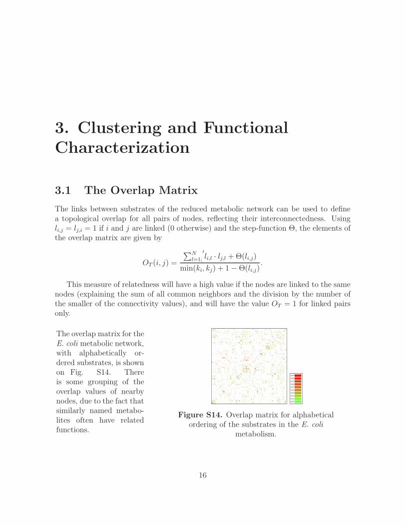
The links between substrates of the reduced metabolic network can be used to definea topological overlap for all pairs of nodes, reflecting their interconnectedness. Usingli,j = lj,i = 1 if i and j are linked (0 otherwise) and the step-function Θ, the elements ofthe overlap matrix are given by

OT (i, j) =

∑Nl=1;

′li,l · lj,l + Θ(li,j)

min(ki, kj) + 1 − Θ(li,j).

This measure of relatedness will have a high value if the nodes are linked to the samenodes (explaining the sum of all common neighbors and the division by the number ofthe smaller of the connectivity values), and will have the value OT = 1 for linked pairsonly.

The overlap matrix for theE. coli metabolic network,with alphabetically or-dered substrates, is shownon Fig. S14. Thereis some grouping of theoverlap values of nearbynodes, due to the fact thatsimilarly named metabo-lites often have relatedfunctions.

0.050 0

0.150 0

0.250 0

0.350 0

0.450 0

0.550 0

0.650 0

0.750 0

0.850 0

0.950 0

Figure S14. Overlap matrix for alphabeticalordering of the substrates in the E. coli

metabolism.

16

3.2 Hierarchical Clustering

Our hierarchical clustering based on the overlap matrix uses the unweighted averagelinkage clustering algorithm, also known as UMPGA [7, 8]. The method finds thelargest overlap present in the matrix, joins the corresponding substrates u and v to abranching point on the tree, and substitutes them with a ”new” cluster {u, v}. Thisnew item in the overlap matrix has the overlap with an arbitrary substrate (cluster) w

O({u, v}, w) =nu · O(u, w) + nv · O(v, w)

nu + nv,

where nu is the number of components in cluster u. This definition ensures that alloriginal overlap values are represented in the joint cluster’s overlap value with the sameweight, explaining the method’s name as “unweighted average linkage clustering”. Therepetition of the above rules eventually shrinks the overlap matrix to a single value,corresponding to the root of the hierarchical tree, thus producing a tree with all theoriginal substrates as its leafs, grouped naturally on branches reflecting their hierarchicaloverlap.

When the overlap values between clusters is redundant (i.e. there are at least twogroups of clusters with the same overlap value) the program automatically joins the pairlocated first. The ordering of two branches under a junction is irrelevant, thus arbitrary.The distance between two junction levels is defined to be one.

The clustering of the E. coli metabolic network, and thus ordering the overlap matrixaccording to a substrate’s horizontal location on the tree, lead to Fig. 4a (article).

3.3 Embedded Modularity of E. Coli Metabolism

Based on its Topological Organisation

At the highest level we find that the E. coli metabolic network is partitioned into threelarge classes, appearing as major branches on the tree (Fig. S15 and Fig. 4a from arti-cle). The smallest of these branches consists of the Coenzyme and Vitamin metabolism(light orange), its inner core is divided into Vitamin K- and Terpene metabolism, whileits outer part is specific to Sirohem Anabolism.

The second major branch represents the nucleotide and nucleic acid metabolism(red). It’s two major sub-branches are clearly divided into the Pyrimidine and Purinemetabolism subclasses. Interestingly, the purine group has a small sub-branch rep-resenting Dihydrofolate Anabolism, a subgroup that is shared with the Coenzyme andVitamin metabolism (light orange) containing metabolites reacting within the subgroup.The strong link to Purine metabolism is due to the dihydroneopterin-triphosphate syn-thesis pathway from GTP.

17

The third and largest branch naturally breaks into a smaller branch containinglargely Carbohydrate metabolism (blue), with most of the poly- and disaccharides in thebranch on the left; while Monosaccharides- (some of which are also present in the leftbranch), Sugar Alcohols, and Alcohol metabolites dominate the right branch. The Mem-brane Lipid metabolism (cyan),(which is fairly independent of the Fatty Acid group) isnested into the Carbohydrates group due to shared glycerol metabolism susbstrates inits biosynthesis pathways. A small group representing Pyridoxine Anabolism (Vitamins:Vitamin 6B, light orange) is linked into this branch via biosynthesis from D-erythrose-4P.Another small nested group is the 3-phosphoshikimate biosynthesis from D-erythrose-4P,a part of Chorismate metabolism shared by both the Aromatic Compounds Metabolism(dark pink), and the Coenzyme group. The second major sub-branch is the least segre-gated one, as in addition to Proteins, Peptides and Amino Acids group (PPA, green) itcontains several apparently unrelated pathways. One clear and separate sub-branch atthe left side represents Fatty Acid metabolism, it being strongly linked to the OrganicAcids and the Citrate Cycle (Carbohydrates, blue). Since almost half of the AminoAcid class substrates are shared with Carbohydrates Metabolism, pathways belongingto Pyruvate, Glyoxylate and Metabolism Sugar Alcohols are naturally grouped withinthe PPA group, appearing as small red branches on the figure. Formate metabolism,which represents almost the complete Monocarbon Compounds Metabolism class (yel-low) is linked to Metabolism Sugar Alcohols. The IMP anabolic pathway (part of Purinemetabolism, blue) starts with 5-phospho-’alpha’-D-ribose-1-diphosphate and the sub-strates on this pathway diverge from Purine metabolism, and are grouped on the PPAbranch. Similarly, Nicotinamide metabolism (Coenzymes, light orange) is grouped intothe PPA branch due to NAD(+) biosynthesis from L-aspartate. Enterobactin biosyn-thesis from chorismate pathway links parts of Chorismate metabolism (Coenzymes, lightorange) to L-serine, the small (2 substrate) insert next to the Pyruvate group (a smallblue group, shared by Carbohydrates and PPA). The pathway leading from L-Glutamateto L-glutamate-1-semialdehyde is part of Lipid, Aromatic Compounds and Coenzymesmetabolism, its links anchor it into Glutamate metabolism. The PPA substrates on thislarge branch tend to group according to classifications based on the names of the aminoacids, but not all of them show up on distinguishable sub-branches. They tend to groupinternally as well, for example most of glutamate and arginine metabolism substratescan be found on the same branch.

18

Nucleic Acids

Dis

acch

arid

es

Mon

osac

char

ides

Mem

bran

e L

ipid

s

Fatty

Aci

ds

Org

anic

Aci

ds

Cys

tein

eL

acta

te

Pyru

vate

Seri

ne, T

hreo

nine

Tyr

osin

e

Nic

otin

amid

e

Puri

ne B

yosy

nthe

sis

Glu

tam

ate

Arg

inin

e

Vita

min

K

Siro

hem

Cho

rism

ate

Vit.Coenz.

Pyri

mid

ine

Puri

ne

Carbohydrates Lipids Amino acids

Form

ate

Met

ab. s

ugar

alc

.

Nucleotides

Gly

coxi

late

Figure S15. Hierarchical tree representing the reduced E. Coli metabolic network.

19

References

[1] A.-L. Barabasi, R. Albert, Science 286, 509-12 (1999).

[2] B. Bollobas, Random Graphs, Academic, London (1985).

[3] M. Girvan, M. E. J. Newman, Community structure in social and biological net-works, Los Alamos Archive cond-mat/0112110 (2001).

[4] D. J. Watts, S. H. Strogatz, Nature 393, 440-2 (1998).

[5] S. N. Dorogovtsev, A. V. Goltsev, J. F. F. Mendez, Pseudofractal Scale-free Web,Los Alamos Archive cond-mat/0112143 (2001).

[6] J. Jeong, B. Tombor, R. Albert, Z. N. Oltvai, A.-L. Barabasi, Nature 407, 651-654(2000).

[7] J. Sokal, P. Sneath, Numerical Taxonomy, Freeman, San Francisco (1973).

[8] M. B. Eisen, P. T. Spellman, P. O. Brown, D. Botstein, Proc Natl Acad Sci USA95, 12863-8 (1998)

20