Embed Size (px)
Citation preview
1
Chapter 10
THE PARTIAL EQUILIBRIUM COMPETITIVE MODEL
Copyright ©2005 by South-Western, a division of Thomson Learning. All rights reserved.

2
Market Demand
• Assume that there are only two goods (x and y)
– An individual’s demand for x is
Quantity of x demanded = x(px,py,I)
– If we use i to reflect each individual in the market, then the market demand curve is
n
iiyxi ppxX
1
),,( for demand Market I

3
Market Demand
• To construct the market demand curve, PX is allowed to vary while Py and the income of each individual are held constant
• If each individual’s demand for x is downward sloping, the market demand curve will also be downward sloping

4
Market Demand
x xx
pxpxpx
x1* x2*
px*
To derive the market demand curve, we sum thequantities demanded at every price
x1
Individual 1’sdemand curve
x2
Individual 2’sdemand curve
Market demandcurve
X*
X
x1* + x2* = X*
5
Shifts in the MarketDemand Curve
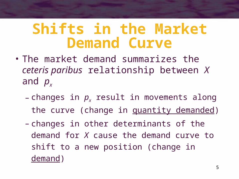
• The market demand summarizes the ceteris paribus relationship between X and px
– changes in px result in movements along the
curve (change in quantity demanded)
– changes in other determinants of the
demand for X cause the demand curve to
shift to a new position (change in demand)
6
Shifts in Market Demand
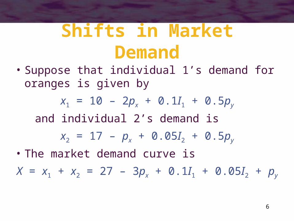
• Suppose that individual 1’s demand for oranges is given by
x1 = 10 – 2px + 0.1I1 + 0.5py
and individual 2’s demand is
x2 = 17 – px + 0.05I2 + 0.5py
• The market demand curve is
X = x1 + x2 = 27 – 3px + 0.1I1 + 0.05I2 + py

7
Shifts in Market Demand
• To graph the demand curve, we must assume values for py, I1, and I2
• If py = 4, I1 = 40, and I2 = 20, the market demand curve becomes
X = 27 – 3px + 4 + 1 + 4 = 36 – 3px
8
Shifts in Market Demand
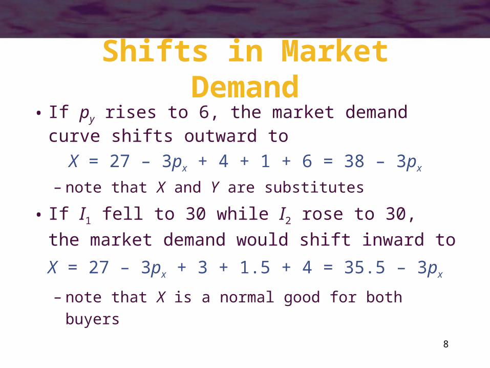
• If py rises to 6, the market demand curve shifts outward to
X = 27 – 3px + 4 + 1 + 6 = 38 – 3px
– note that X and Y are substitutes
• If I1 fell to 30 while I2 rose to 30, the market
demand would shift inward to
X = 27 – 3px + 3 + 1.5 + 4 = 35.5 – 3px
– note that X is a normal good for both buyers

9
Generalizations
• Suppose that there are n goods (xi, i = 1,n) with prices pi, i = 1,n.
• Assume that there are m individuals in the economy
• The j th’s demand for the i th good will depend on all prices and on Ij
xij = xij(p1,…,pn, Ij)
10
Generalizations
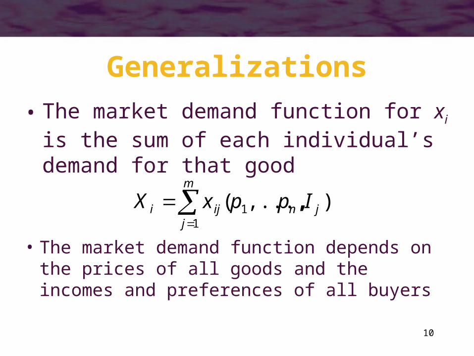
• The market demand function for xi is the sum of each individual’s demand for that good
),,...,( 11
jn
m
jiji ppxX I
• The market demand function depends on the prices of all goods and the incomes and preferences of all buyers

11
Elasticity of Market Demand• The price elasticity of market demand is
measured by
D
DPQ Q
P
P
PPQe
),',(
,
I
• Market demand is characterized by whether demand is elastic (eQ,P <-1) or inelastic (0> eQ,P > -1)
12
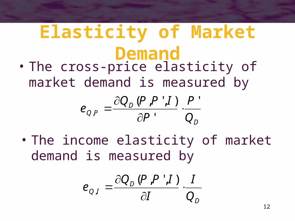
Elasticity of Market Demand• The cross-price elasticity of market
demand is measured by
D
DPQ Q
P
P
PPQe
'
'
),',(,
I
• The income elasticity of market demand is measured by
D
DQ Q
PPQe
II
II
),',(
,

13
Timing of the Supply Response• In the analysis of competitive pricing, the
time period under consideration is important– very short run
• no supply response (quantity supplied is fixed)
– short run• existing firms can alter their quantity supplied, but
no new firms can enter the industry
– long run• new firms may enter an industry

14
Pricing in the Very Short Run
• In the very short run (or the market period), there is no supply response to changing market conditions– price acts only as a device to ration demand
• price will adjust to clear the market
– the supply curve is a vertical line

15
Pricing in the Very Short Run
Quantity
Price
S
D
Q*
P1
D’
P2
When quantity is fixed in thevery short run, price will risefrom P1 to P2 when the demandrises from D to D’
16
Short-Run Price Determination
• The number of firms in an industry is fixed
• These firms are able to adjust the quantity they are producing– they can do this by altering the levels of the
variable inputs they employ
17
Perfect Competition• A perfectly competitive industry is one
that obeys the following assumptions:– there are a large number of firms, each
producing the same homogeneous product– each firm attempts to maximize profits– each firm is a price taker
• its actions have no effect on the market price
– information is perfect– transactions are costless
18
Short-Run Market Supply• The quantity of output supplied to the
entire market in the short run is the sum of the quantities supplied by each firm– the amount supplied by each firm depends
on price
• The short-run market supply curve will be upward-sloping because each firm’s short-run supply curve has a positive slope
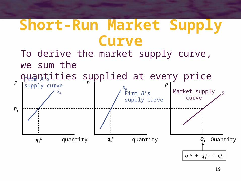
19
Short-Run Market Supply Curve
quantity Quantityquantity
PPP
q1A q1
B
P1
To derive the market supply curve, we sum thequantities supplied at every price
sA
Firm A’ssupply curve sB
Firm B’ssupply curve
Market supplycurve
Q1
S
q1A + q1
B = Q1
20
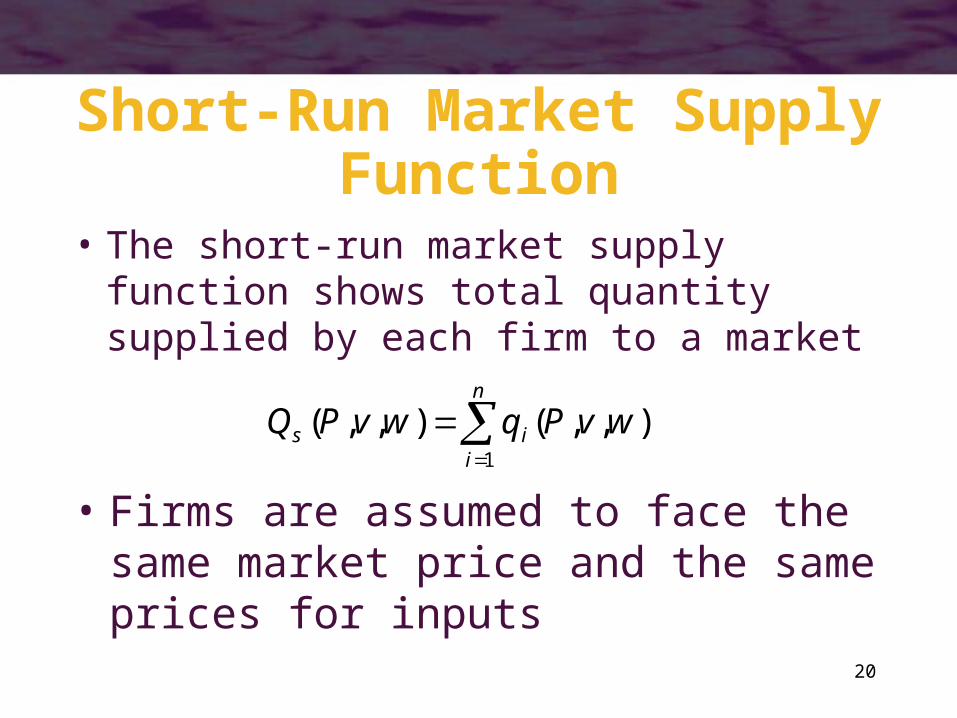
Short-Run Market Supply Function
• The short-run market supply function shows total quantity supplied by each firm to a market
n
iis wvPqwvPQ
1
),,(),,(
• Firms are assumed to face the same market price and the same prices for inputs

21
Short-Run Supply Elasticity
• The short-run supply elasticity describes the responsiveness of quantity supplied to changes in market price
S
SPS Q
P
P
Q
P
Qe
in change %
supplied in change %,
• Because price and quantity supplied are positively related, eS,P > 0

22
A Short-Run Supply Function
• Suppose that there are 100 identical firms each with the following short-run supply curve
qi (P,v,w) = 10P/3 (i = 1,2,…,100)
• This means that the market supply function is given by
3
1000
3
10100
1
100
1
PPqQ
i iis

23
A Short-Run Supply Function
• In this case, computation of the elasticity of supply shows that it is unit elastic
13/10003
1000),,(,
P
P
Q
P
P
wvPQe
S
SPS
24
Equilibrium Price Determination
• An equilibrium price is one at which quantity demanded is equal to quantity supplied– neither suppliers nor demanders have an
incentive to alter their economic decisions
• An equilibrium price (P*) solves the equation:
),*,(),'*,( wvPQPPQ SD I
25
Equilibrium Price Determination
• The equilibrium price depends on many exogenous factors– changes in any of these factors will likely
result in a new equilibrium price
26
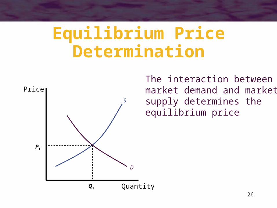
Equilibrium Price Determination
Quantity
Price
S
D
Q1
P1
The interaction betweenmarket demand and marketsupply determines theequilibrium price

27
Market Reaction to aShift in Demand
Quantity
Price
S
D
Q1
P1
Q2
P2 Equilibrium price andequilibrium quantity willboth rise
If many buyers experiencean increase in their demands,the market demand curvewill shift to the right
D’
28
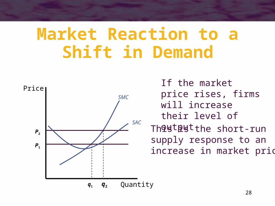
Market Reaction to aShift in Demand
Quantity
PriceSMC
q1
P1
This is the short-runsupply response to anincrease in market price
q2
P2
If the market price rises, firms will increase their level of output
SAC
29
Shifts in Supply and Demand Curves
• Demand curves shift because– incomes change– prices of substitutes or complements change– preferences change
• Supply curves shift because– input prices change– technology changes– number of producers change
30
Shifts in Supply and Demand Curves
• When either a supply curve or a demand curve shift, equilibrium price and quantity will change
• The relative magnitudes of these changes depends on the shapes of the supply and demand curves

31
Shifts in Supply
Quantity Quantity
PricePriceS
S’S
S’
DD
PP
Q
P’
Q’
P’
QQ’
Elastic Demand Inelastic Demand
Small increase in price,large drop in quantity
Large increase in price,small drop in quantity

32
Shifts in Demand
Quantity Quantity
PricePrice
S
S
D D
P P
Q
P’
Q’
P’
Q Q’
Elastic Supply Inelastic Supply
Small increase in price,large rise in quantity
Large increase in price,small rise in quantity
D’ D’

33
Changing Short-Run Equilibria
• Suppose that the market demand for luxury beach towels is
QD = 10,000 – 500P
and the short-run market supply is
QS = 1,000P/3
• Setting these equal, we find
P* = $12
Q* = 4,000
34
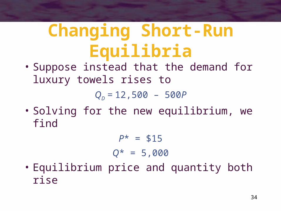
Changing Short-Run Equilibria
• Suppose instead that the demand for luxury towels rises to
QD = 12,500 – 500P
• Solving for the new equilibrium, we find
P* = $15
Q* = 5,000
• Equilibrium price and quantity both rise

35
Changing Short-Run Equilibria• Suppose that the wage of towel cutters
rises so that the short-run market supply becomes
QS = 800P/3
• Solving for the new equilibrium, we find
P* = $13.04
Q* = 3,480
• Equilibrium price rises and quantity falls

36
Mathematical Model of Supply and Demand
• Suppose that the demand function is represented by
QD = D(P,)
is a parameter that shifts the demand curveD/ = D can have any sign
D/P = DP < 0
37
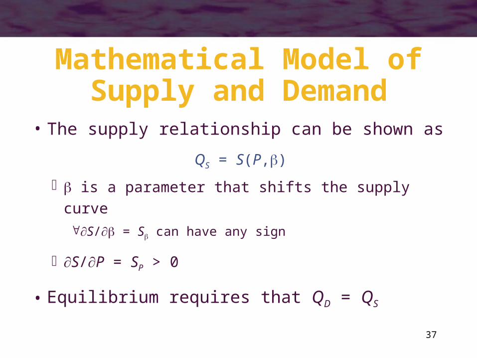
Mathematical Model of Supply and Demand
• The supply relationship can be shown as
QS = S(P,)
is a parameter that shifts the supply curve
S/ = S can have any sign
S/P = SP > 0
• Equilibrium requires that QD = QS
38
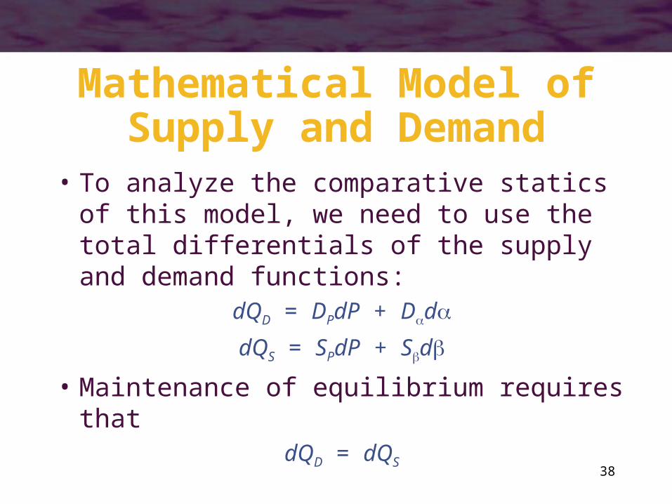
Mathematical Model of Supply and Demand
• To analyze the comparative statics of this model, we need to use the total differentials of the supply and demand functions:
dQD = DPdP + Dd
dQS = SPdP + Sd
• Maintenance of equilibrium requires thatdQD = dQS

39
Mathematical Model of Supply and Demand
• Suppose that the demand parameter () changed while remains constant
• The equilibrium condition requires thatDPdP + Dd = SPdP
PP DS
DP
• Because SP - DP > 0, P/ will have the same sign as D

40
Mathematical Model of Supply and Demand
• We can convert our analysis to elasticities
PDS
D
P
Pe
PPP
,
PQPS
Q
PP
P ee
e
QP
DS
QD
e,,
,,
)(

41
Long-Run Analysis• In the long run, a firm may adapt all of its
inputs to fit market conditions– profit-maximization for a price-taking firm
implies that price is equal to long-run MC
• Firms can also enter and exit an industry in the long run– perfect competition assumes that there are
no special costs of entering or exiting an industry
42
Long-Run Analysis• New firms will be lured into any market
for which economic profits are greater than zero– entry of firms will cause the short-run
industry supply curve to shift outward– market price and profits will fall– the process will continue until economic
profits are zero

43
Long-Run Analysis
• Existing firms will leave any industry for which economic profits are negative– exit of firms will cause the short-run industry
supply curve to shift inward– market price will rise and losses will fall– the process will continue until economic
profits are zero

44
Long-Run Competitive Equilibrium
• A perfectly competitive industry is in long-run equilibrium if there are no incentives for profit-maximizing firms to enter or to leave the industry– this will occur when the number of firms is
such that P = MC = AC and each firm operates at minimum AC
45
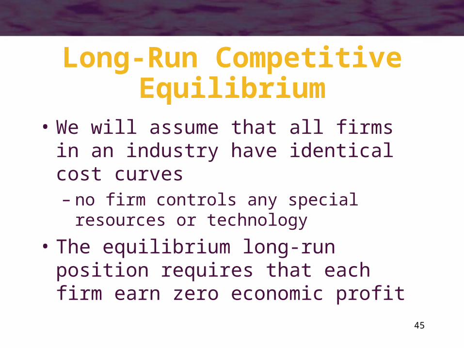
Long-Run Competitive Equilibrium
• We will assume that all firms in an industry have identical cost curves– no firm controls any special resources or
technology
• The equilibrium long-run position requires that each firm earn zero economic profit

46
Long-Run Equilibrium: Constant-Cost Case
• Assume that the entry of new firms in an industry has no effect on the cost of inputs– no matter how many firms enter or leave
an industry, a firm’s cost curves will remain unchanged
• This is referred to as a constant-cost industry

47
Long-Run Equilibrium: Constant-Cost Case
A Typical Firm Total MarketQuantity Quantity
SMC MC
AC
S
D
q1
P1
Q1
This is a long-run equilibrium for this industry
P = MC = ACPrice Price
48
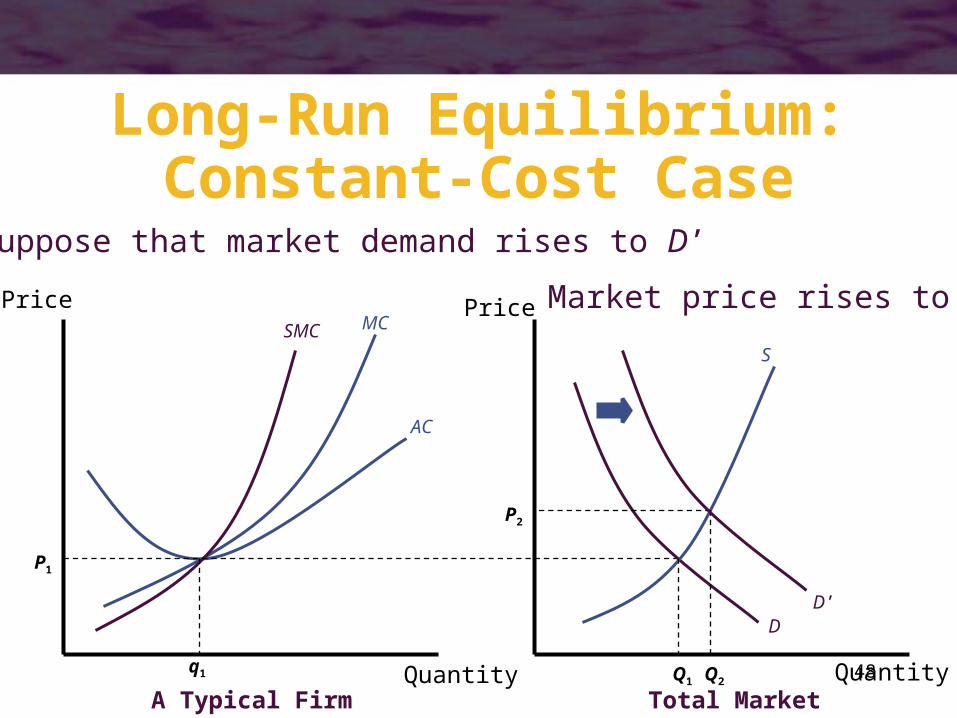
Long-Run Equilibrium: Constant-Cost Case
A Typical Firm Total Market
q1 Quantity Quantity
SMC MC
AC
S
D
P1
Q1
P2
Market price rises to P2
Q2
Suppose that market demand rises to D’
D’
Price Price
49
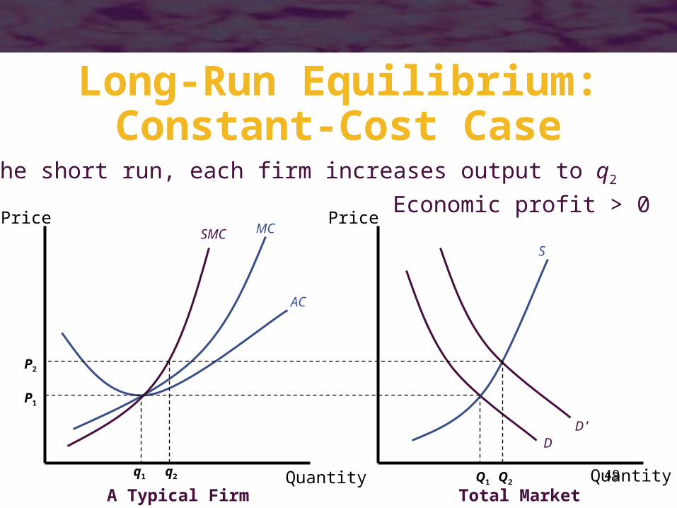
Long-Run Equilibrium: Constant-Cost Case
A Typical Firm Total Market
q1 Quantity Quantity
SMC MC
AC
S
D
P1
Q1
D’
P2
Economic profit > 0
Q2
In the short run, each firm increases output to q2
q2
Price Price
50
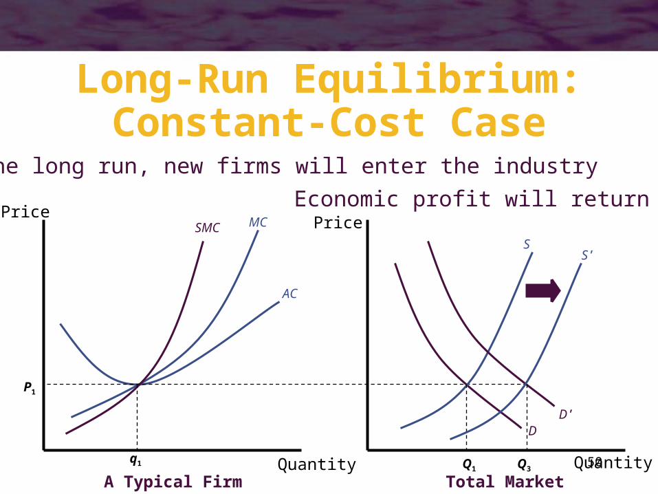
Long-Run Equilibrium: Constant-Cost Case
A Typical Firm Total Market
q1 Quantity Quantity
SMC MC
AC
S
D
P1
Q1
D’
Economic profit will return to 0
Q3
In the long run, new firms will enter the industry
S’
PricePrice

51
Long-Run Equilibrium: Constant-Cost Case
A Typical Firm Total Market
q1 Quantity Quantity
SMC MC
AC
S
D
P1
Q1
D’
Q3
S’
The long-run supply curve will be a horizontal line (infinitely elastic) at p1
LS
Price Price

52
Infinitely Elastic Long-Run Supply
• Suppose that the total cost curve for a typical firm in the bicycle industry is
TC = q3 – 20q2 + 100q + 8,000
• Demand for bicycles is given by
QD = 2,500 – 3P

53
Infinitely Elastic Long-Run Supply
• To find the long-run equilibrium for this market, we must find the low point on the typical firm’s average cost curve– where AC = MC
AC = q2 – 20q + 100 + 8,000/q
MC = 3q2 – 40q + 100– this occurs where q = 20
• If q = 20, AC = MC = $500– this will be the long-run equilibrium price
54
Shape of the Long-Run Supply Curve
• The zero-profit condition is the factor that determines the shape of the long-run cost curve– if average costs are constant as firms enter,
long-run supply will be horizontal– if average costs rise as firms enter, long-run
supply will have an upward slope– if average costs fall as firms enter, long-run
supply will be negatively sloped

55
Long-Run Equilibrium: Increasing-Cost Industry
• The entry of new firms may cause the average costs of all firms to rise– prices of scarce inputs may rise– new firms may impose “external” costs on
existing firms– new firms may increase the demand for
tax-financed services

56
Long-Run Equilibrium: Increasing-Cost Industry
A Typical Firm (before entry) Total Market
q1 Quantity Quantity
SMC MC
AC
S
D
P1
Q1
Suppose that we are in long-run equilibrium in this industry
P = MC = ACPricePrice

57
Long-Run Equilibrium: Increasing-Cost Industry
A Typical Firm (before entry) Total Market
q1 Quantity Quantity
SMC MC
AC
S
D
P1
Q1
Suppose that market demand rises to D’
D’
P2
Market price rises to P2 and firms increase output to q2
Q2q2
Price Price

58
Long-Run Equilibrium: Increasing-Cost Industry
A Typical Firm (after entry) Total MarketQuantity Quantity
SMC’ MC’
AC’
S
D
P1
Q1
D’
q3
P3
Entry of firms causes costs for each firm to rise
Q3
Positive profits attract new firms and supply shifts out
S’
Price Price

59
Long-Run Equilibrium: Increasing-Cost Industry
A Typical Firm (after entry) Total Market
q3 Quantity Quantity
SMC’ MC’
AC’
S
D
p1
Q1
D’
p3
Q3
S’
The long-run supply curve will be upward-sloping
LS
Price Price
60
Long-Run Equilibrium: Decreasing-Cost Industry
• The entry of new firms may cause the average costs of all firms to fall– new firms may attract a larger pool of
trained labor– entry of new firms may provide a “critical
mass” of industrialization• permits the development of more efficient
transportation and communications networks

61
Long-Run Equilibrium: Decreasing-Cost Case
A Typical Firm (before entry) Total Market
q1 Quantity Quantity
SMC MC
AC
S
D
P1
Q1
Suppose that we are in long-run equilibrium in this industry
P = MC = ACPrice Price

62
Long-Run Equilibrium: Decreasing-Cost Industry
A Typical Firm (before entry) Total Market
q1 Quantity Quantity
SMC MC
AC
S
D
P1
Q1
Suppose that market demand rises to D’
D’
P2
Market price rises to P2 and firms increase output to q2
Q2q2
Price Price

63
Long-Run Equilibrium: Decreasing-Cost Industry
A Typical Firm (before entry) Total Market
q1 Quantity Quantity
SMC’MC’
AC’
S
D
P1
Q1
D’P3
Entry of firms causes costs for each firm to fall
Q3q3
Positive profits attract new firms and supply shifts out
S’
PricePrice

64
Long-Run Equilibrium: Decreasing-Cost Industry
A Typical Firm (before entry) Total Market
q1 Quantity Quantity
SMC’MC’
AC’
S
D
P1
Q1
The long-run industry supply curve will be downward-sloping
D’P3
Q3q3
S’
LS
Price Price
65
Classification of Long-Run Supply Curves
• Constant Cost– entry does not affect input costs– the long-run supply curve is horizontal at
the long-run equilibrium price
• Increasing Cost– entry increases inputs costs– the long-run supply curve is positively
sloped

66
Classification of Long-Run Supply Curves
• Decreasing Cost– entry reduces input costs– the long-run supply curve is negatively
sloped

67
Long-Run Elasticity of Supply
• The long-run elasticity of supply (eLS,P) records the proportionate change in long-run industry output to a proportionate change in price
LS
LSPLS Q
P
P
Q
P
Qe
in change %
in change %,
• eLS,P can be positive or negative
– the sign depends on whether the industry exhibits increasing or decreasing costs

68
Comparative Statics Analysis of Long-Run Equilibrium
• Comparative statics analysis of long-run equilibria can be conducted using estimates of long-run elasticities of supply and demand
• Remember that, in the long run, the number of firms in the industry will vary from one long-run equilibrium to another
69
Comparative Statics Analysis of Long-Run Equilibrium
• Assume that we are examining a constant-cost industry
• Suppose that the initial long-run equilibrium industry output is Q0 and the typical firm’s output is q* (where AC is minimized)
• The equilibrium number of firms in the industry (n0) is Q0/q*
70
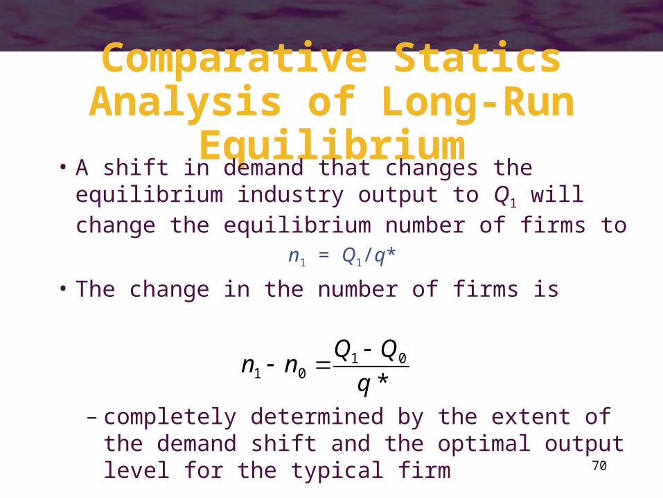
Comparative Statics Analysis of Long-Run Equilibrium
• A shift in demand that changes the equilibrium industry output to Q1 will change the equilibrium number of firms to
n1 = Q1/q*
• The change in the number of firms is
*q
QQnn 01
01
– completely determined by the extent of the demand shift and the optimal output level for the typical firm

71
Comparative Statics Analysis of Long-Run Equilibrium
• The effect of a change in input prices is more complicated– we need to know how much minimum
average cost is affected– we need to know how an increase in long-
run equilibrium price will affect quantity demanded
72
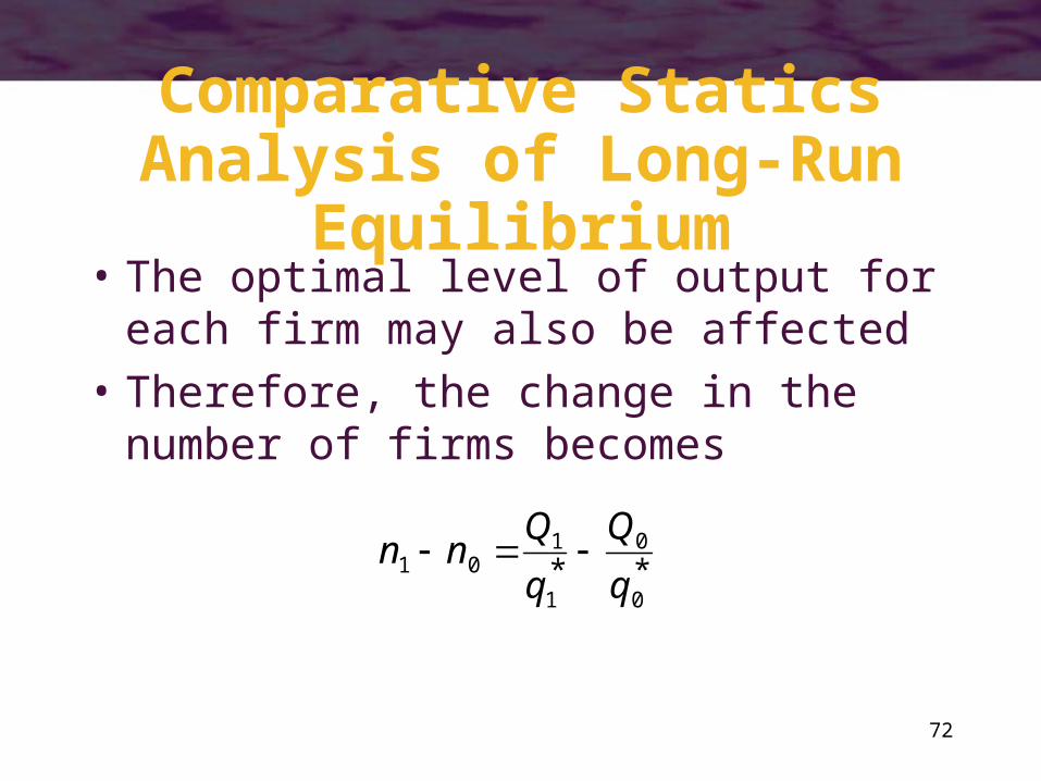
Comparative Statics Analysis of Long-Run Equilibrium
• The optimal level of output for each firm may also be affected
• Therefore, the change in the number of firms becomes
**
0
0
1
101
q
Q
q
Qnn

73
Rising Input Costs and Industry Structure
• Suppose that the total cost curve for a typical firm in the bicycle industry is
TC = q3 – 20q2 + 100q + 8,000
and then rises to
TC = q3 – 20q2 + 100q + 11,616
• The optimal scale of each firm rises from 20 to 22 (where MC = AC)

74
Rising Input Costs and Industry Structure
• At q = 22, MC = AC = $672 so the long-run equilibrium price will be $672
• If demand can be represented byQD = 2,500 – 3P
then QD = 484
• This means that the industry will have 22 firms (484 22)

75
Producer Surplus in the Long Run
• Short-run producer surplus represents the return to a firm’s owners in excess of what would be earned if output was zero– the sum of short-run profits and fixed costs
76
Producer Surplus in the Long Run
• In the long-run, all profits are zero and there are no fixed costs– owners are indifferent about whether they
are in a particular market• they could earn identical returns on their
investments elsewhere
• Suppliers of inputs may not be indifferent about the level of production in an industry
77
Producer Surplus in the Long Run
• In the constant-cost case, input prices are assumed to be independent of the level of production– inputs can earn the same amount in
alternative occupations
• In the increasing-cost case, entry will bid up some input prices– suppliers of these inputs will be made better
off

78
Producer Surplus in the Long Run
• Long-run producer surplus represents the additional returns to the inputs in an industry in excess of what these inputs would earn if industry output was zero– the area above the long-run supply curve
and below the market price• this would equal zero in the case of constant
costs

79
Ricardian Rent• Long-run producer surplus can be most
easily illustrated with a situation first described by economist David Ricardo– assume that there are many parcels of land
on which a particular crop may be grown• the land ranges from very fertile land (low costs
of production) to very poor, dry land (high costs of production)

80
Ricardian Rent• At low prices only the best land is used
• Higher prices lead to an increase in output through the use of higher-cost land– the long-run supply curve is upward-sloping
because of the increased costs of using less fertile land

81
Ricardian Rent
Low-Cost Firm Total Marketq* Quantity Quantity
MC
AC
S
D
P*
Q*
The owners of low-cost firms will earn positive profits
Price Price

82
Ricardian Rent
Marginal Firm Total Marketq* Quantity Quantity
MC
AC
S
D
P*
Q*
The owners of the marginal firm will earn zero profit
Price Price

83
Ricardian Rent
• Firms with higher costs (than the marginal firm) will stay out of the market– would incur losses at a price of P*
• Profits earned by intramarginal firms can persist in the long run– they reflect a return to a unique resource
• The sum of these long-run profits constitutes long-run producer surplus
84
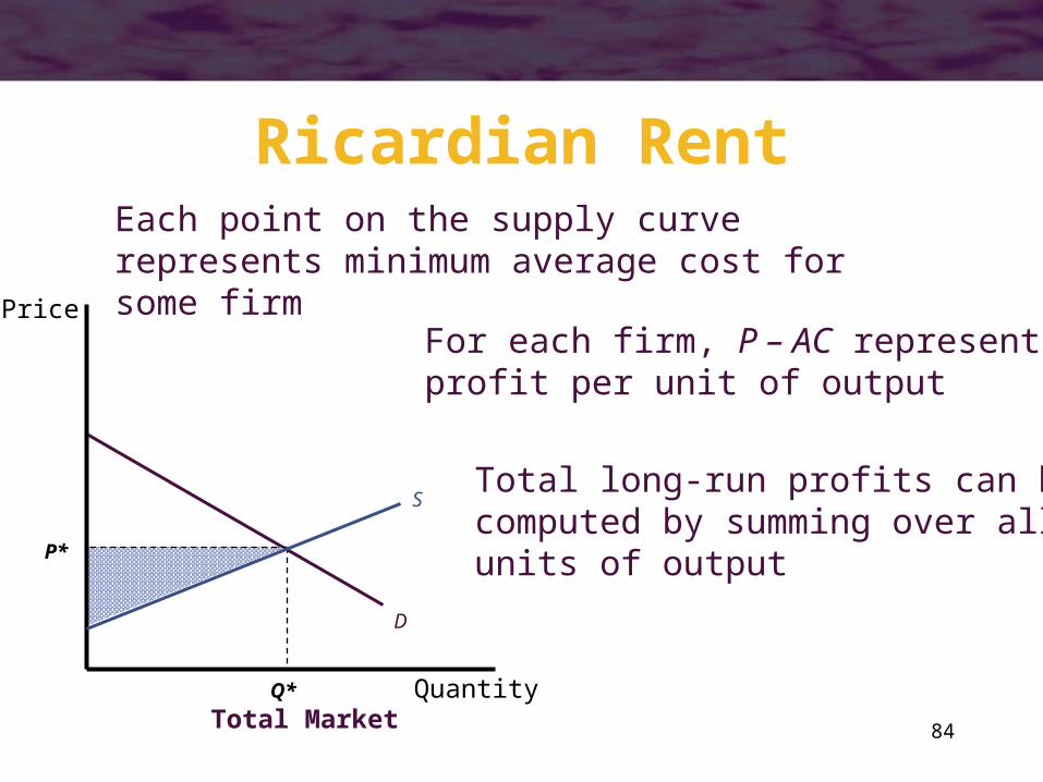
Ricardian Rent
For each firm, P – AC representsprofit per unit of output
Total MarketQuantity
S
D
P*
Q*
Each point on the supply curve represents minimum average cost for some firm
Total long-run profits can becomputed by summing over allunits of output
Price

85
Ricardian Rent
• The long-run profits for the low-cost firms will often be reflected in the prices of the unique resources owned by those firms– the more fertile the land is, the higher its
price
• Thus, profits are said to be capitalized inputs’ prices– reflect the present value of all future profits
86
Ricardian Rent
• It is the scarcity of low-cost inputs that creates the possibility of Ricardian rent
• In industries with upward-sloping long-run supply curves, increases in output not only raise firms’ costs but also generate factor rents for inputs
87
Important Points to Note:• In the short run, equilibrium prices are
established by the intersection of what demanders are willing to pay (as reflected by the demand curve) and what firms are willing to produce (as reflected by the short-run supply curve)– these prices are treated as fixed in both
demanders’ and suppliers’ decision-making processes
88
Important Points to Note:• A shift in either demand or supply will
cause the equilibrium price to change– the extent of such a change will depend on
the slopes of the various curves
• Firms may earn positive profits in the short run– because fixed costs must always be paid,
firms will choose a positive output as long as revenues exceed variable costs

89
Important Points to Note:• In the long run, the number of firms is
variable in response to profit opportunities– the assumption of free entry and exit implies
that firms in a competitive industry will earn zero economic profits in the long run (P = AC)
– because firms also seek maximum profits, the equality P = AC = MC implies that firms will operate at the low points of their long-run average cost curves

90
Important Points to Note:• The shape of the long-run supply curve
depends on how entry and exit affect firms’ input costs– in the constant-cost case, input prices do not
change and the long-run supply curve is horizontal
– if entry raises input costs, the long-run supply curve will have a positive slope
91
Important Points to Note:
• Changes in long-run market equilibrium will also change the number of firms– precise predictions about the extent of these
changes is made difficult by the possibility that the minimum average cost level of output may be affected by changes in input costs or by technical progress

92
Important Points to Note:
• If changes in the long-run equilibrium in a market change the prices of inputs to that market, the welfare of the suppliers of these inputs will be affected– such changes can be measured by changes
in the value of long-run producer surplus