1

Chapter 5 – Orthogonality and Least Squares

Outline5.1 Orthonormal Bases and Orthogonal Projections5.2 Gram-Schmidt Process and QR Factorization5.3 Orthogonal Transformations and Orthogonal Matrices5.4 Least Squares and Data Fitting5.5 Inner Product Spaces

2

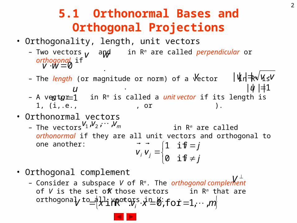
5.1 Orthonormal Bases and Orthogonal Projections

• Orthogonality, length, unit vectors– Two vectors and in Rn are called perpendicular or orthogonal if

.

– The length (or magnitude or norm) of a vector in Rn is .

– A vector in Rn is called a unit vector if its length is 1, (i,.e., , or ).

• Orthonormal vectors– The vectors in Rn are called orthonormal if they are all

unit vectors and orthogonal to one another:

• Orthogonal complement– Consider a subspace V of Rn. The orthogonal complement of V is the

set of those vectors in Rn that are orthogonal to all vectors in V:

v

w

0wv

v

vvv

||||u 1|||| u

1uu

mvvv

,,, 21

ji

jivv ji if0

if1

Vx

mixvxV in ,,1for ,0 :Rin

3

Orthonormal Vectors

• Orthonormal vectors are linearly independent.

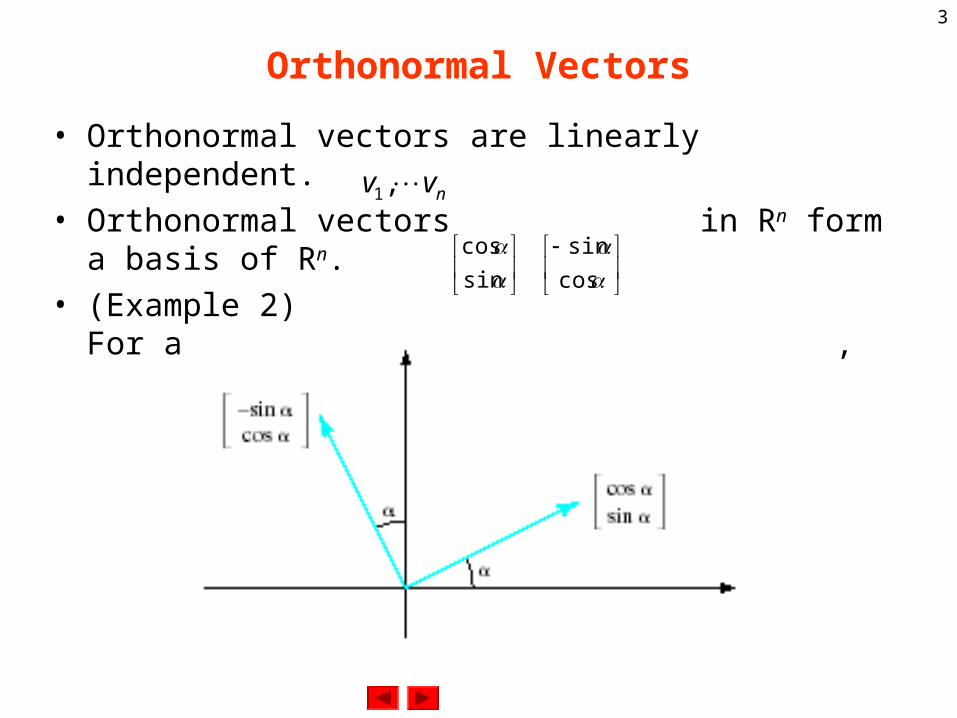
• Orthonormal vectors in Rn form a basis of Rn.

• (Example 2)For any scalar , the vectors , are orthonormal.

sin

cos

nvv

,1

cos

sin

4

Orthogonal Projections

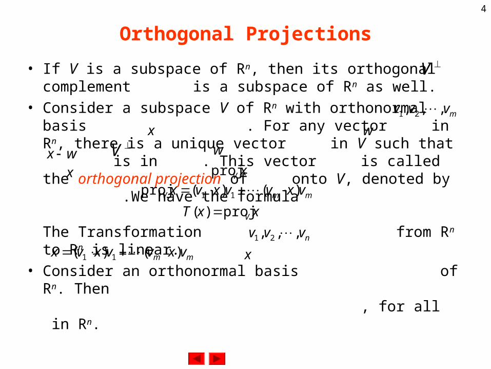
• If V is a subspace of Rn, then its orthogonal complement is a subspace of Rn as well.

• Consider a subspace V of Rn with orthonormal basis . For any vector in Rn, there is a unique vector in V such that is in . This vector is called the orthogonal projection of onto V, denoted by .We have the formula

The Transformation from Rn to Rn is linear.

• Consider an orthonormal basis of Rn. Then , for all in Rn.

V

V

mvvv

,,, 21

x

w

wx

w

x xV

proj

mmV vxvvxvx

)()(proj 11

xxT V

proj)(

nvvv

,,, 21

mm vxvvxvx

)()( 11 x

5

Example 4

•

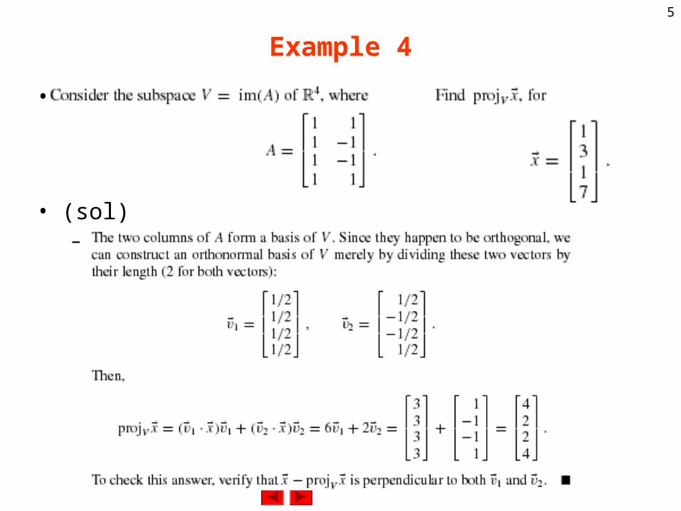
• (sol)–

6

Pythagorean Theorem

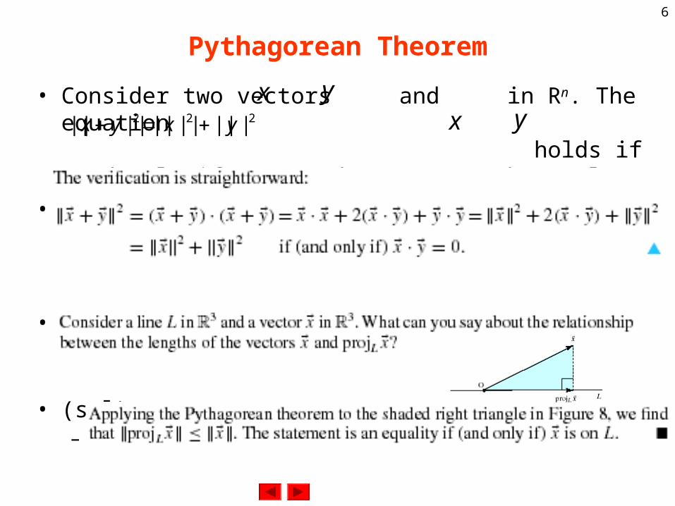
• Consider two vectors and in Rn. The equation holds if (and only if) and are orthogonal.

•

• Example 6

• (sol)–

x

y

222 |||||||||||| yxyx

x

y

7

Projections

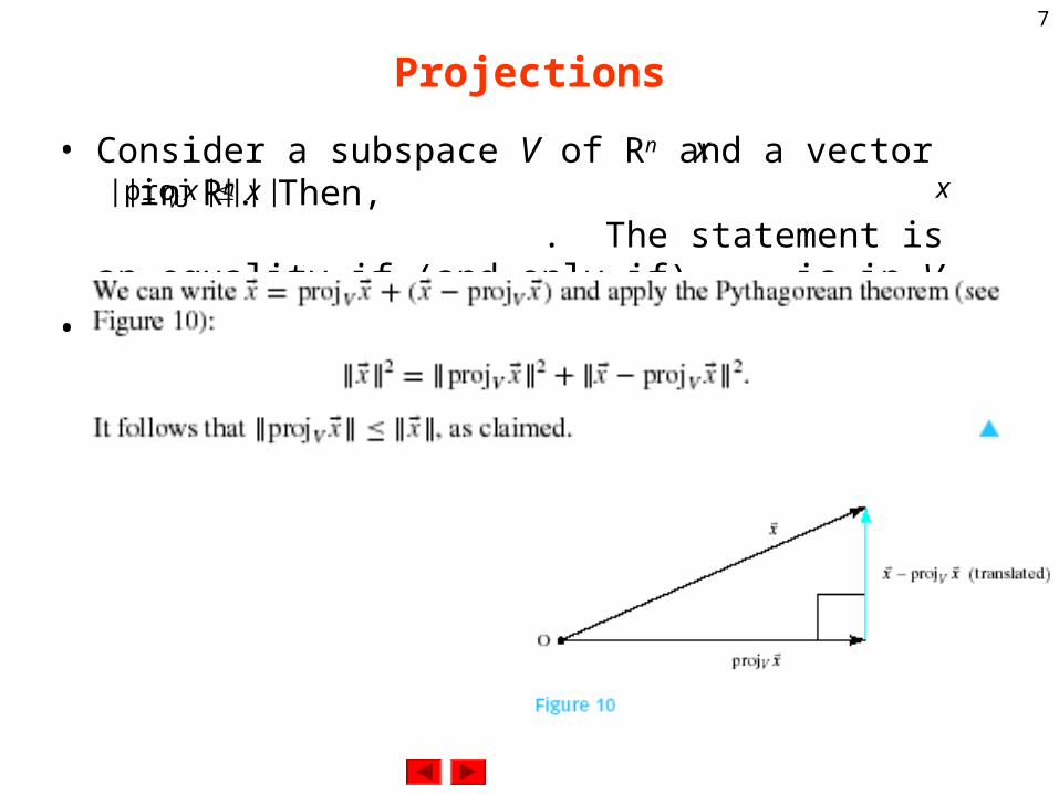
• Consider a subspace V of Rn and a vector in Rn. Then, . The statement is an equality if (and only if) is in V.

•

x

x

||||||proj|| xxV

8

Cauchy–Schwarz Inequality

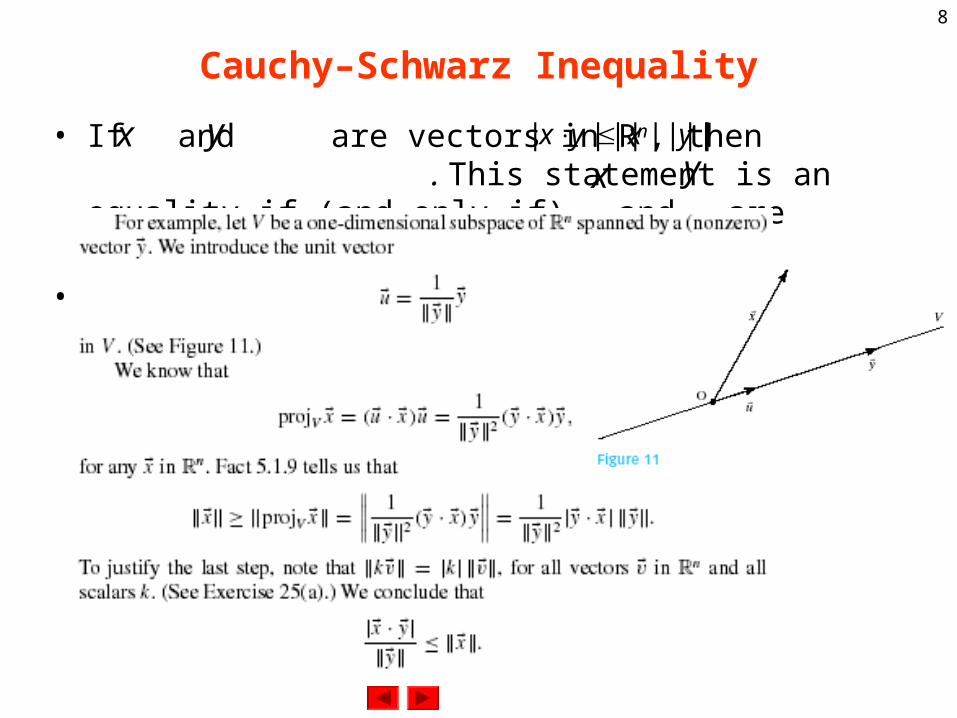
• If and are vectors in Rn, then . This statement is an equality if (and only if) and are parallel.

•

x

y

|||||||||| yxyx

x y

9

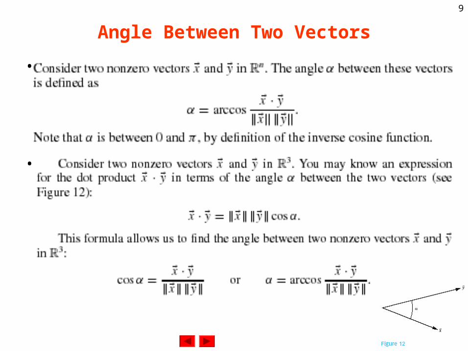
Angle Between Two Vectors

•

•

10

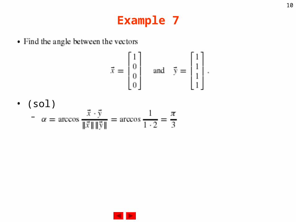
Example 7

•

• (sol)–

11

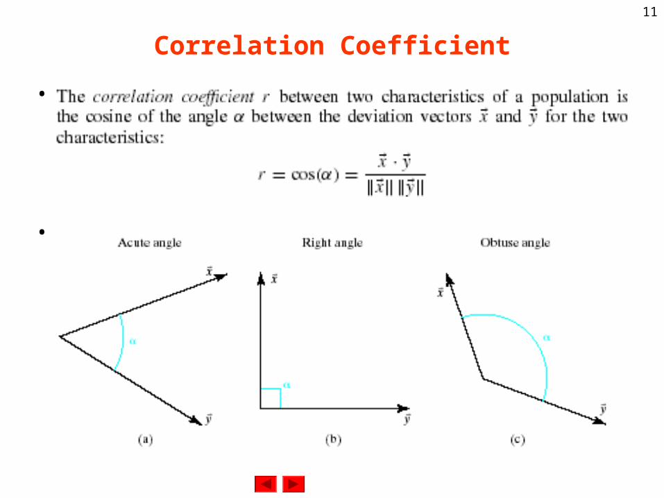
Correlation Coefficient

•

•

12

Correlation

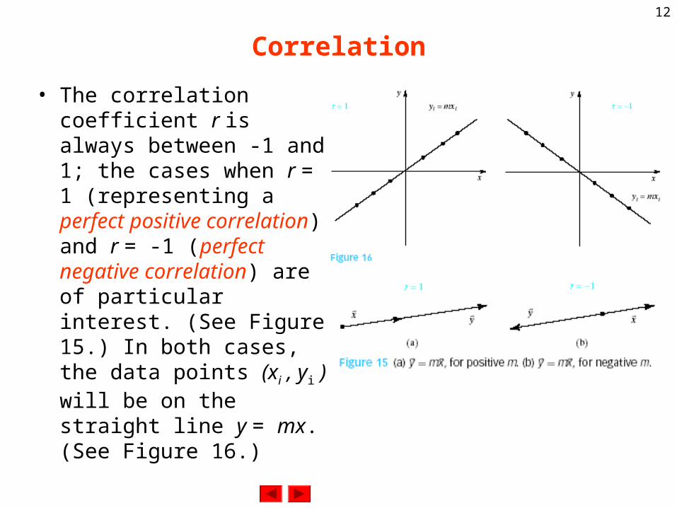
• The correlation coefficient r is always between -1 and 1; the cases when r = 1 (representing a perfect positive correlation) and r = -1 (perfect negative correlation) are of particular interest. (See Figure 15.) In both cases, the data points (xi , yi ) will be on the straight line y = mx. (See Figure 16.)

13

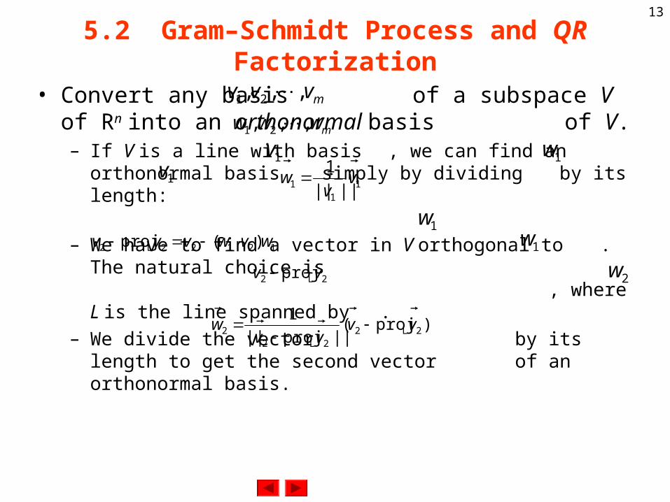
5.2 Gram–Schmidt Process and QR Factorization

• Convert any basis of a subspace V of Rn into an orthonormal basis of V.– If V is a line with basis , we can find an orthonormal basis simply

by dividing by its length:

– We have to find a vector in V orthogonal to . The natural choice is , where L is the line spanned by .

– We divide the vector by its length to get the second vector of an orthonormal basis.

mwww

,,, 21

mvvv

,,, 21

1v

1w

1v

11

1 ||||

1v

vw

1w

1w

12122L2 )(proj wvwvvv

2w

2L2 proj vv

)proj(||proj||

12L2

2L22 vv

vvw

14

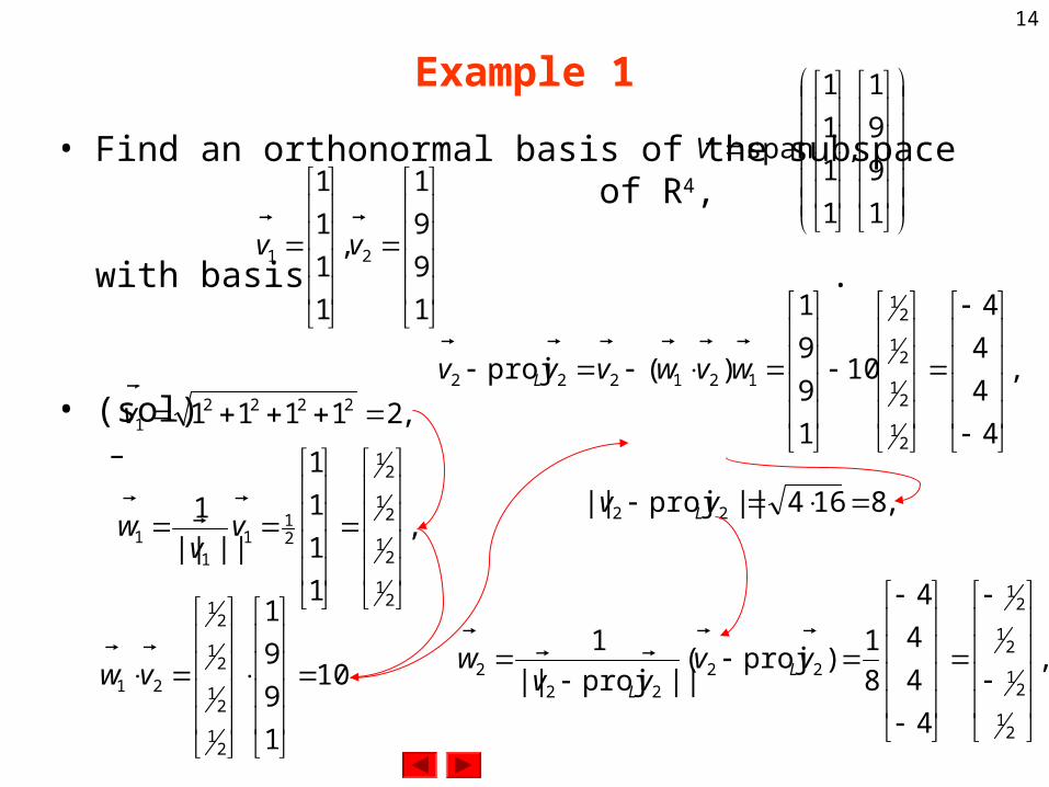
Example 1

• Find an orthonormal basis of the subspace of R4,

with basis .

• (sol)–

1

9

9

1

,

1

1

1

1

spanV

1

9

9

1

,

1

1

1

1

21 vv

,21111 22221 v

,

1

1

1

1

||||

1

21

21

21

21

21

11

1

vv

w

10

1

9

9

1

21

21

21

21

21

vw

,

4

4

4

4

10

1

9

9

1

)(proj

21

21

21

21

121222

wvwvvv L

,8164||proj|| 22 vv L

,

4

4

4

4

8

1)proj(

||proj||

1

21

21

21

21

2222

2

vvvv

w LL

15

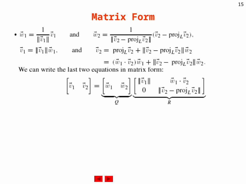
Matrix Form

•

16

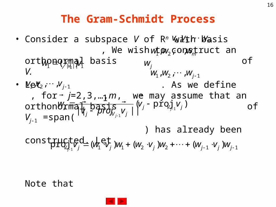
The Gram-Schmidt Process

• Consider a subspace V of Rn with basis , We wish to construct an orthonormal basis of V.

• Let . As we define , for j=2,3,…,m, we may assume that an orthonormal basis of Vj-1 =span( ) has already been constructed. Let

Note that

mvvv

,,, 21

mwww

,,, 21

1||||1

1 )(1

vw v

jw

121 ,,, jwww

121 ,,, jvvv

)proj(||||

11

1

jVjjVj

j vvvprojv

wj

j

112211 )()()(proj1

jjjjjjV wvwwvwwvwvj

17

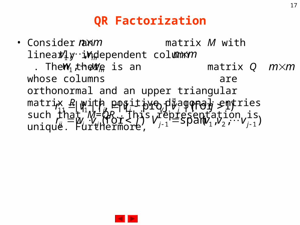
QR Factorization

• Consider an matrix M with linearly independent column . Then there is an matrix Q whose columns are orthonormal and an upper triangularmatrix R with positive diagonal entries such that M=QR. This representation is unique. Furthermore,

mnmvv

,,1

mww

,,1 mmmn

),1for (||proj||||,||1111

jvvrvr jVjjj j

%

),for ( jivwr jiij

),,(span 1211 jj vvvV

18

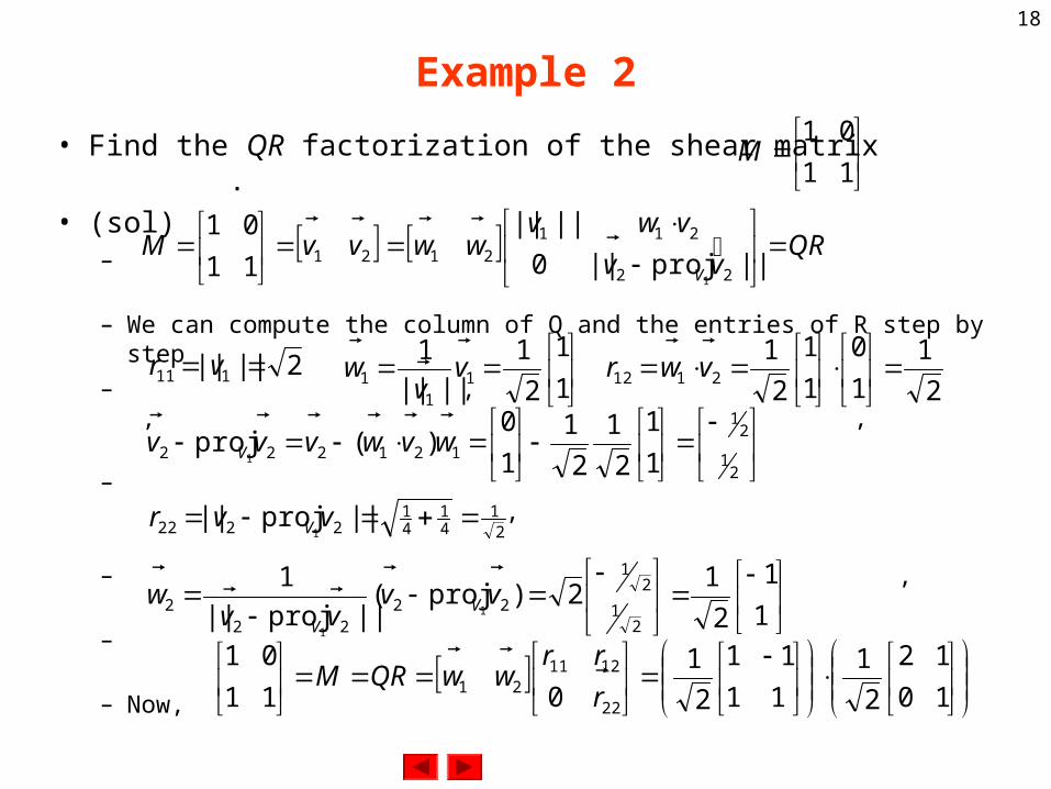
Example 2

• Find the QR factorization of the shear matrix .

• (sol)–

– We can compute the column of Q and the entries of R step by step

– , , ,

– ,

– ,

–

– Now,

11

01M

QRvv

vwvwwvvM

V

||proj||0

||||

11

01

22

211

2121

1

%

2|||| 111 vr

1

1

2

1

||||

11

11 v

vw

2

1

1

0

1

1

2

12112

vwr

21

21

121222 1

1

2

1

2

1

1

0)(proj

1wvwvvv V

21

41

41

2222 ||proj||1

vvr V

1

1

2

12)proj(

||proj||

1

21

21

2222

2 1

1

vvvv

w VV

10

12

2

1

11

11

2

1

011

01

22

121121 r

rrwwQRM

19

5.3 Orthogonal Transformation and Orthogonal Matrices

• A linear transformation T from Rn to Rn is called orthogonal if it preserves the length of vectors:

If is an orthogonal transformation, we say that A is an orthogonal matrix.

nxxxT Rin allfor ,||||||)(||

xAxT

)(

20

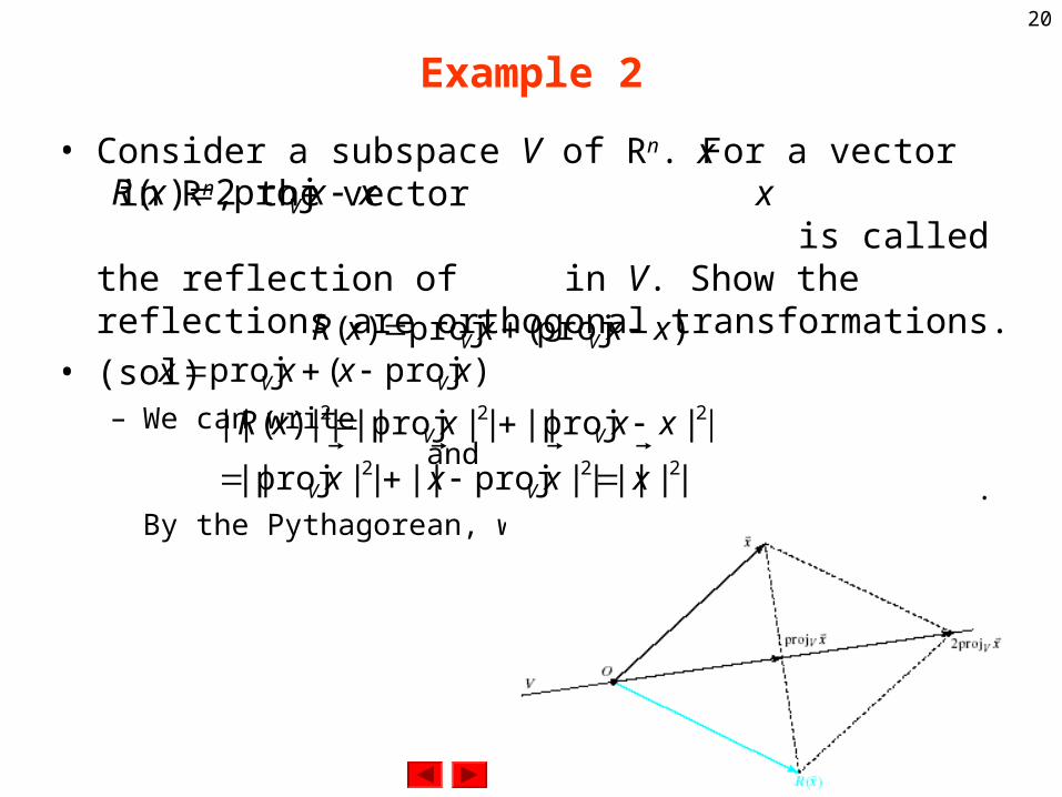
Example 2

• Consider a subspace V of Rn. For a vector in Rn, the vector is called the reflection of in V. Show the reflections are orthogonal transformations.

• (sol)– We can write and

. By the Pythagorean, we have

x

xxxR V

proj2)(

)proj(proj)( xxxxR VV

)proj(proj xxxx VV

222

222

||||||proj||||proj||

||proj||||proj||||)(||

xxxx

xxxxR

VV

VV

x

21

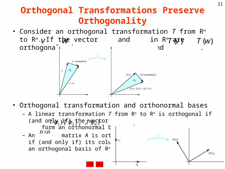
Orthogonal Transformations Preserve Orthogonality

• Consider an orthogonal transformation T from Rn to Rn. If the vector and in Rn are orthogonal, then so are and .

• Orthogonal transformation and orthonormal bases– A linear transformation T from Rn to Rn is orthogonal if (and only if) the

vector form an orthonormal basis of Rn.

– An matrix A is orthogonalif (and only if) its columns forman orthogonal basis of Rn.

v

w

)(vT

)(wT

)(,),(),( 21 neTeTeT

nn

22

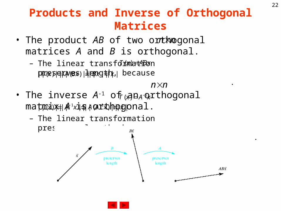
Products and Inverse of Orthogonal Matrices

• The product AB of two orthogonal matrices A and B is orthogonal.– The linear transformation preserves length, because

.

• The inverse A-1 of an orthogonal matrix A is orthogonal.– The linear transformation preserves length, because

.

nn

xABxT

)(

||||||||||)(||||)(|| xxBxBAxT

xAxT 1)(

||||||)(||||||||)(|| 11 xxAAxAxT

nn

23

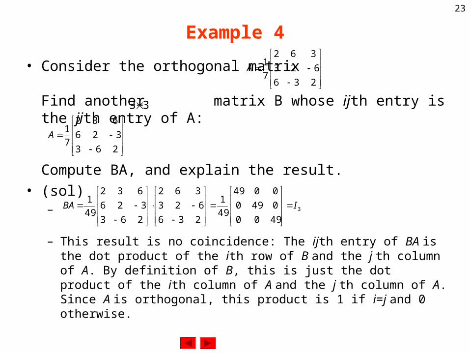
Example 4

• Consider the orthogonal matrix

Find another matrix B whose ijth entry is the jith entry of A:

Compute BA, and explain the result.

• (sol)–

– This result is no coincidence: The ijth entry of BA is the dot product of the ith row of B and the j th column of A. By definition of B, this is just the dot product of the ith column of A and the j th column of A. Since A is orthogonal, this product is 1 if i=j and 0 otherwise.

236

623

362

7

1A

33

263

326

632

7

1A

3

4900

0490

0049

49

1

236

623

362

263

326

632

49

1IBA

24

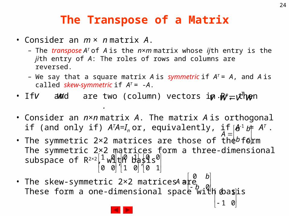
The Transpose of a Matrix

• Consider an m × n matrix A.– The transpose AT of A is the n×m matrix whose ijth entry is the jith entry

of A: The roles of rows and columns are reversed.

– We say that a square matrix A is symmetric if AT = A, and A is called skew-symmetric if AT = -A.

• If and are two (column) vectors in Rn, then .

• Consider an n×n matrix A. The matrix A is orthogonal if (and only if) ATA=In or, equivalently, if A-1 = AT .

• The symmetric 2×2 matrices are those of the formThe symmetric 2×2 matrices form a three-dimensional subspace of R2×2, with basis

• The skew-symmetric 2×2 matrices are These form a one-dimensional space with basis

v

w

wvwv T

cb

baA

10

00,

01

10,

00

01

0

0

b

bA

01

10

25

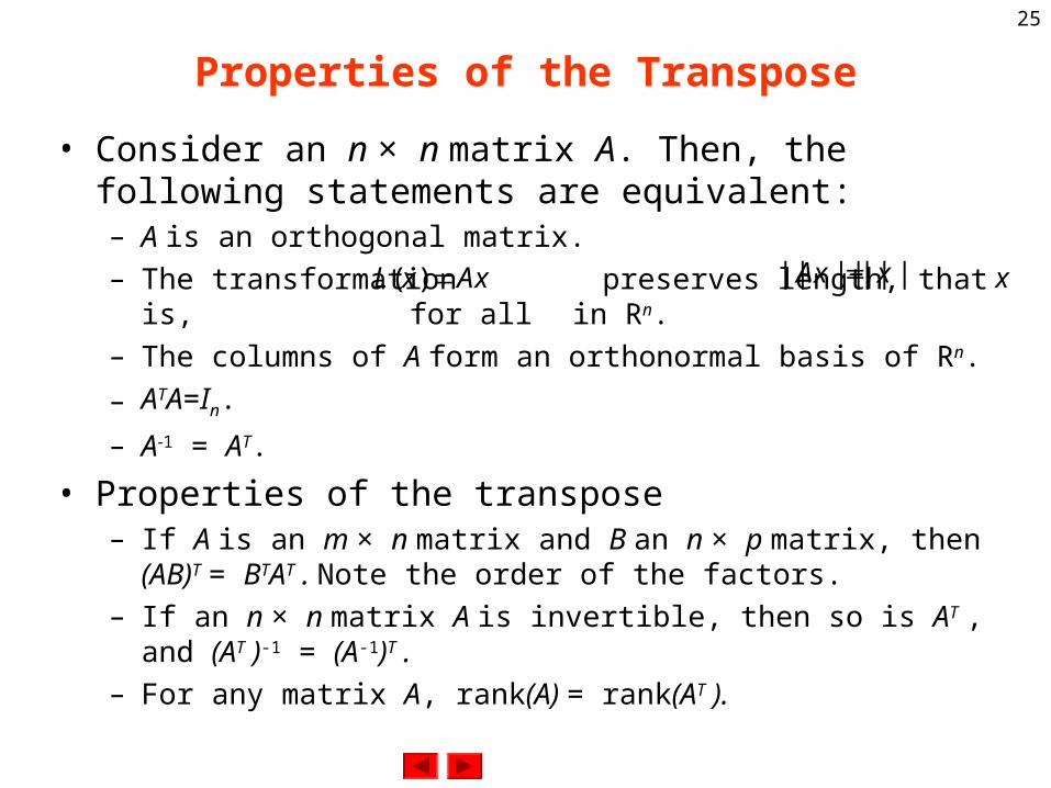
Properties of the Transpose

• Consider an n × n matrix A. Then, the following statements are equivalent:– A is an orthogonal matrix.

– The transformation preserves length, that is, for all in Rn.

– The columns of A form an orthonormal basis of Rn.

– ATA=In.

– A-1 = AT.

• Properties of the transpose– If A is an m × n matrix and B an n × p matrix, then (AB)T = BTAT . Note

the order of the factors.

– If an n × n matrix A is invertible, then so is AT , and (AT )-1 = (A-1)T .

– For any matrix A, rank(A) = rank(AT ).

xAxL

)( |||||||| xxA

x

26

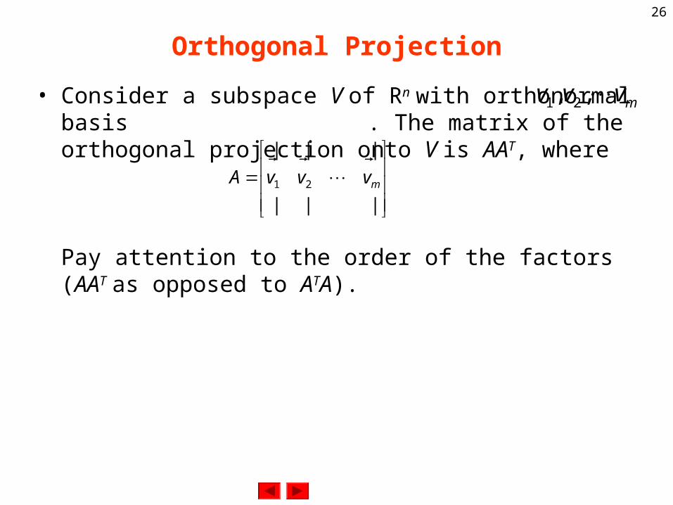
Orthogonal Projection

• Consider a subspace V of Rn with orthonormal basis . The matrix of the orthogonal projection onto V is AAT, where

Pay attention to the order of the factors (AAT as opposed to ATA).

mvvv

,, 21

|||

|||

21 mvvvA

27

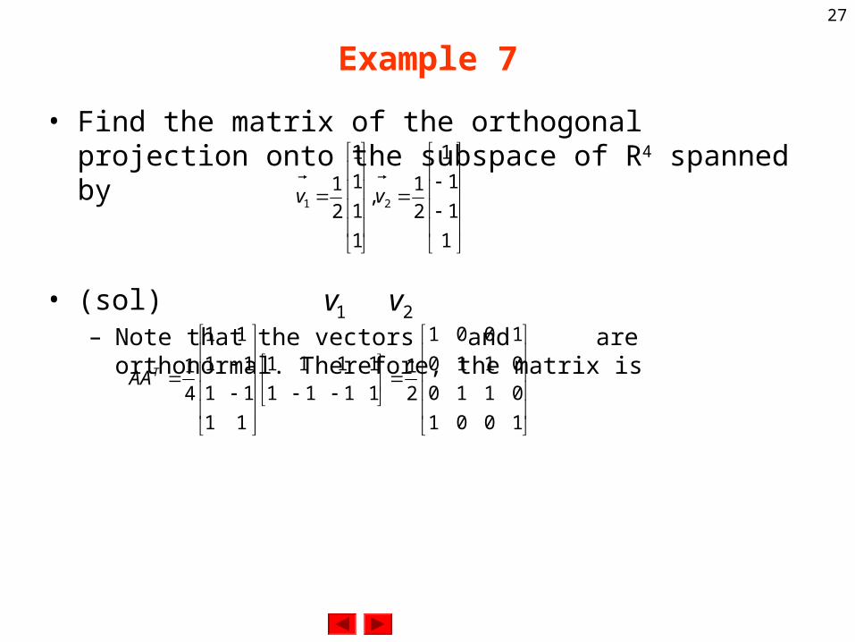
Example 7

• Find the matrix of the orthogonal projection onto the subspace of R4 spanned by

• (sol)– Note that the vectors and are orthonormal. Therefore, the matrix is

1

1

1

1

2

1,

1

1

1

1

2

121 vv

1v

2v

1001

0110

0110

1001

2

1

1111

1111

11

11

11

11

4

1TAA

28

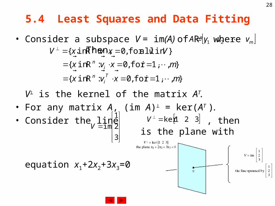
5.4 Least Squares and Data Fitting

• Consider a subspace V = im(A) of Rn, where . Then,

V⊥ is the kernel of the matrix AT.

• For any matrix A, (im A)⊥ = ker(AT ).

• Consider the line , then is the plane with

equation x1+2x2+3x3=0

mvvvA

21

},1,for ,0 :Rin {

},1,for ,0 :Rin {

}in allfor ,0 :Rin {

mixvx

mixvx

VvxvxV

Ti

n

in

n

3

2

1

imV 321kerV

29

Properties of Orthogonal Complement

• Consider a subspace V of Rn. Then,– dim(V) + dim(V⊥) = n,

– (V⊥)⊥ = V,

– V ∩ V⊥ = {0}.

• If A is an m × n matrix, then ker(A) = ker(ATA).

• If A is an m × n matrix with ker(A) = {0}, then ATA is invertible.

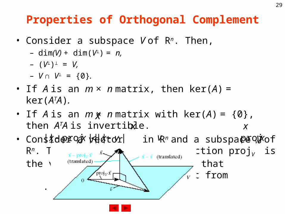
• Consider a vector in Rn and a subspace V of Rn. Then, the orthogonal projection projV is the vector in V closest to , in that , for all in V different from .

x

x

x

||||||proj|| vxxx V

v

xV

proj

30

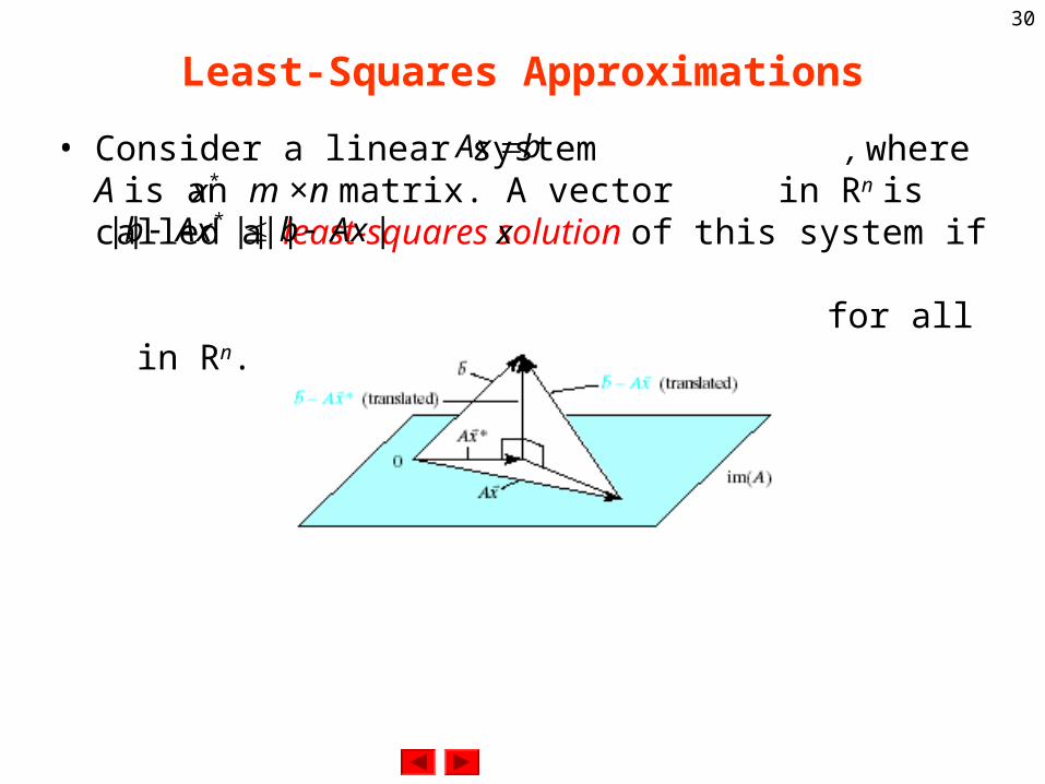
Least-Squares Approximations

• Consider a linear system , where A is an m ×n matrix. A vector in Rn is called a least-squares solution of this system if for all in Rn.

bxA

*x

|||||||| * xAbxAb

x

31

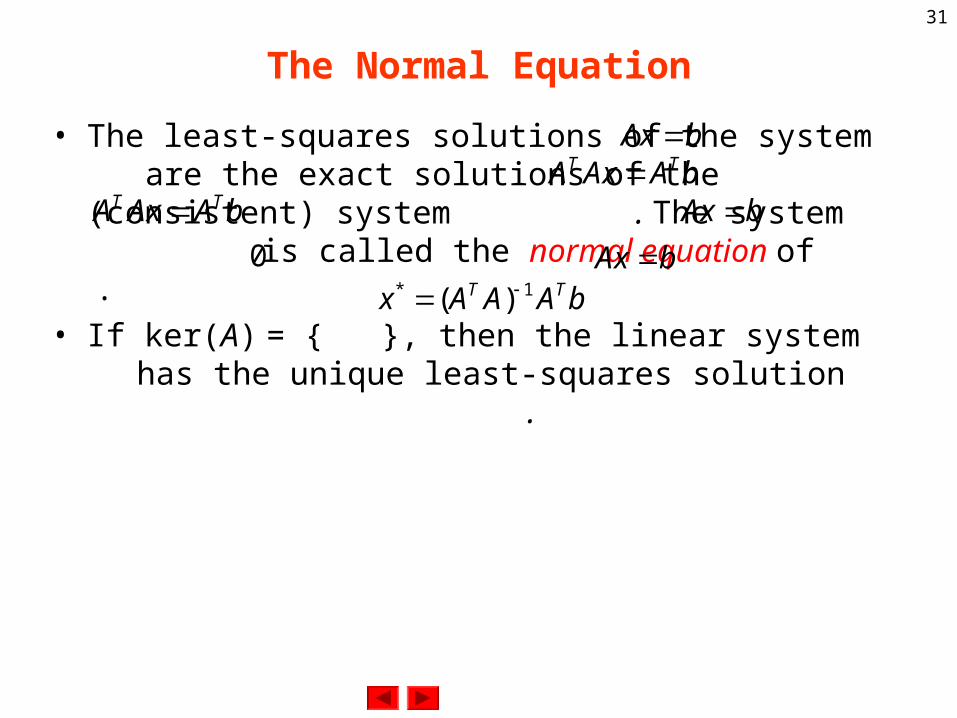
The Normal Equation

• The least-squares solutions of the system are the exact solutions of the (consistent) system . The system is called the normal equation of .

• If ker(A) = { }, then the linear system has the unique least-squares solution .

bxA

bAxAA TT

bAxAA TT

bxA

0

bxA

bAAAx TT 1* )(

32

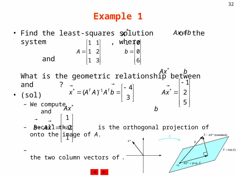
Example 1

• Find the least-squares solution of the system , where

and

What is the geometric relationship between and ?

• (sol)– We compute and

– Recall that is the orthogonal projection of onto the image of A.

– is indeed perpendicular to the two column vectors of A.

*x

bxA

31

21

11

A

6

0

0

b

b

*xA

3

4)( 1* bAAAx TT

5

2

1*xA

*xA

b

1

2

1*xAb

33

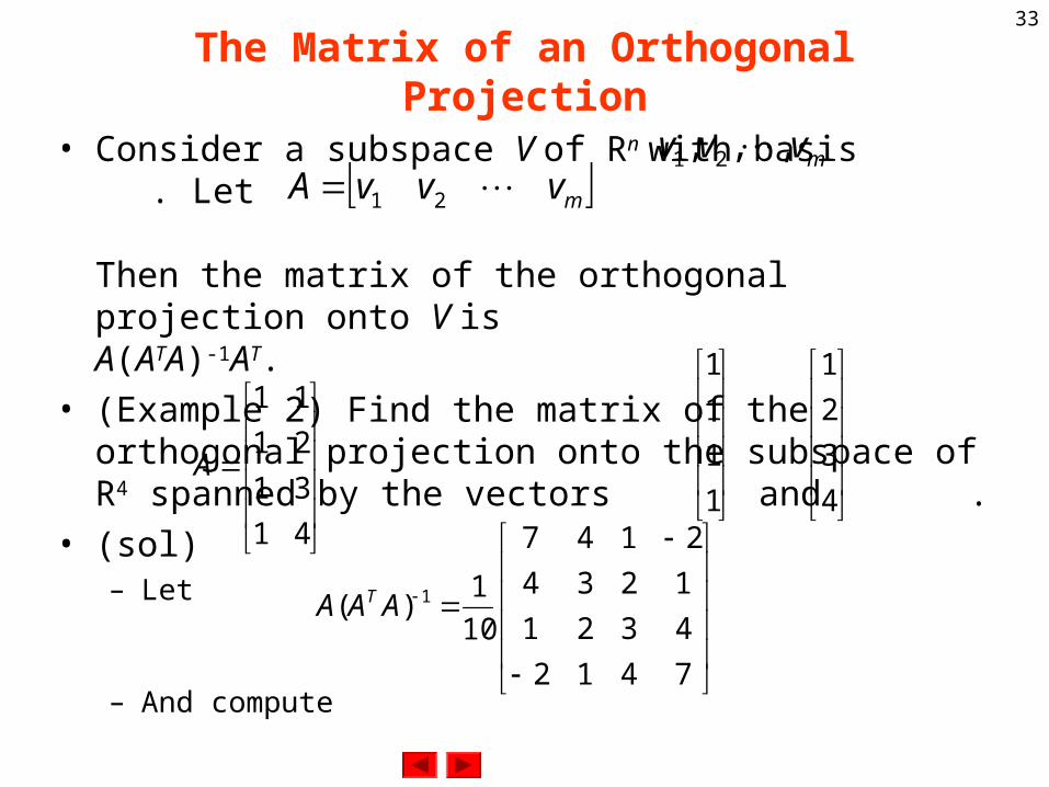
The Matrix of an Orthogonal Projection

• Consider a subspace V of Rn with basis . Let

Then the matrix of the orthogonal projection onto V isA(ATA)-1AT.

• (Example 2) Find the matrix of the orthogonal projection onto the subspace of R4 spanned by the vectors and .

• (sol)– Let

– And compute

mvvv

,,, 21

mvvvA

21

1

1

1

1

4

3

2

1

41

31

21

11

A

7412

4321

1234

2147

10

1)( 1AAA T

34

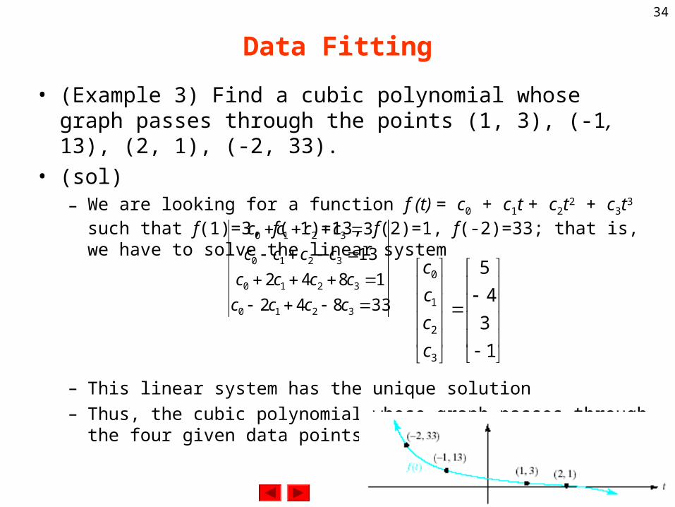
Data Fitting

• (Example 3) Find a cubic polynomial whose graph passes through the points (1, 3), (-1, 13), (2, 1), (-2, 33).

• (sol)– We are looking for a function f (t) = c0 + c1t + c2t2 + c3t3 such that f(1)=3,

f(-1)=13, f(2)=1, f(-2)=33; that is, we have to solve the linear system

– This linear system has the unique solution

– Thus, the cubic polynomial whose graph passes through the four given data points is f (t)=5-4t+3t2-t3,

1

3

4

5

3

2

1

0

c

c

c

c

33842

1842

13

3

3210

3210

3210

3210

cccc

cccc

cccc

cccc

35

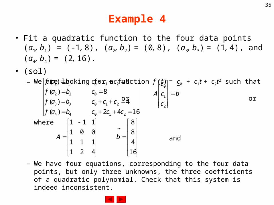
Example 4

• Fit a quadratic function to the four data points (a1, b1) = (-1, 8), (a2, b2) = (0, 8), (a3, b3) = (1, 4), and (a4, b4) = (2, 16).

• (sol)– We are looking for a function f (t) = c0 + c1t + c2t2 such that

or or

where

and

– We have four equations, corresponding to the four data points, but only three unknowns, the three coefficients of a quadratic polynomial. Check that this system is indeed inconsistent.

44

33

22

11

)(

)(

)(

)(

baf

baf

baf

baf

1642

4

8

8

210

210

0

210

ccc

ccc

c

ccc

b

c

c

c

A

2

1

0

421

111

001

111

A

16

4

8

8

b

36

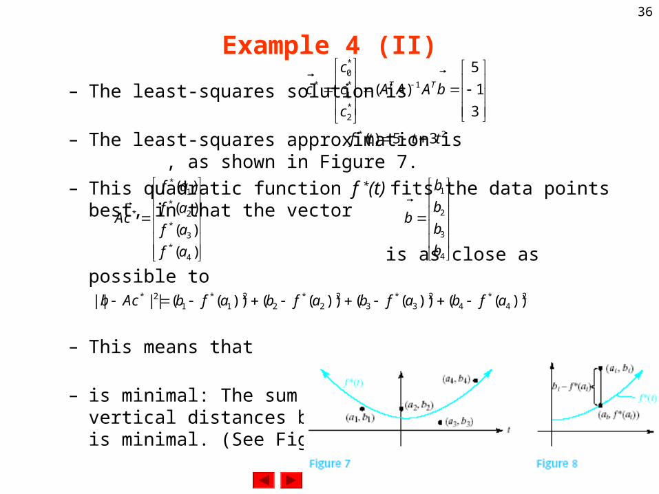
Example 4 (II)

– The least-squares solution is

– The least-squares approximation is , as shown in Figure 7.

– This quadratic function f *(t) fits the data points best, in that the vector

is as close as possible to

– This means that

– is minimal: The sum of the squares of the vertical distances between graph and data points is minimal. (See Figure 8.)

3

1

5

)( 1

*2

*1

*0

* bAAA

c

c

c

c TT

2* 35)( tttf

)(

)(

)(

)(

4*

3*

2*

1*

*

af

af

af

af

cA

4

3

2

1

b

b

b

b

b

24

*4

23

*3

22

*2

21

*1

2* ))(())(())(())((|||| afbafbafbafbcAb

37

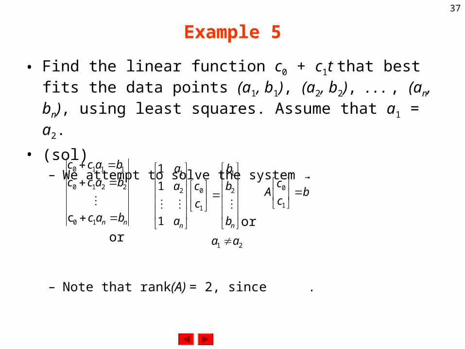
Example 5

• Find the linear function c0 + c1t that best fits the data points (a1, b1), (a2, b2), . . . , (an, bn), using least squares. Assume that a1 = a2.

• (sol)– We attempt to solve the system

or or

– Note that rank(A) = 2, since .

nn bac

bacc

bacc

10

2210

1110

c

nn b

b

b

c

c

a

a

a

2

1

1

02

1

1

1

1

bc

cA

1

0

21 aa

38

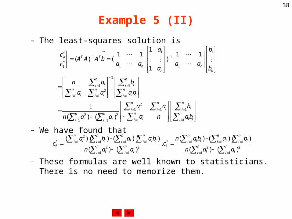
Example 5 (II)

– The least-squares solution is

– We have found that

– These formulas are well known to statisticians. There is no need to memorize them.

i

n

i i

n

i in

i i

n

i i

n

i i

n

i i

n

i i

i

n

i i

n

i in

i i

n

i i

n

i i

nn

nn

TT

ba

b

na

aa

aan

ba

b

aa

an

b

b

aaa

a

aabAAA

c

c

1

1

1

11

2

2

11

2

1

1

1

1

2

1

1

1

1

11

1

1

*1

*0

)()(

1

11)

1

111

()(

2

11

2

111*12

11

2

1111

2*0

)()(

))((-)( ,

)()(

))((-))((

n

i i

n

i i

n

i i

n

i i

n

i ii

n

i i

n

i i

i

n

i i

n

i i

n

i i

n

i i

aan

babanc

aan

baabac

39

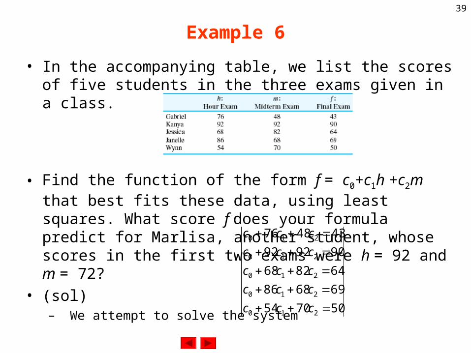
Example 6

• In the accompanying table, we list the scores of five students in the three exams given in a class.

• Find the function of the form f = c0+c1h +c2m that best fits these data, using least squares. What score f does your formula predict for Marlisa, another student, whose scores in the first two exams were h = 92 and m = 72?

• (sol)– We attempt to solve the system

507054

696886

648268

909292

434876

210

210

210

210

210

ccc

ccc

ccc

ccc

ccc

40

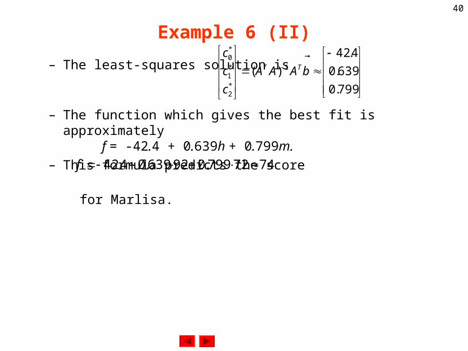
Example 6 (II)

– The least-squares solution is

– The function which gives the best fit is approximately f = -42.4 + 0.639h + 0.799m.

– This formula predicts the score

for Marlisa.

799.0

639.0

4.42

)( 1

*2

*1

*0

bAAA

c

c

cTT

7472799.092639.04.42 f

41

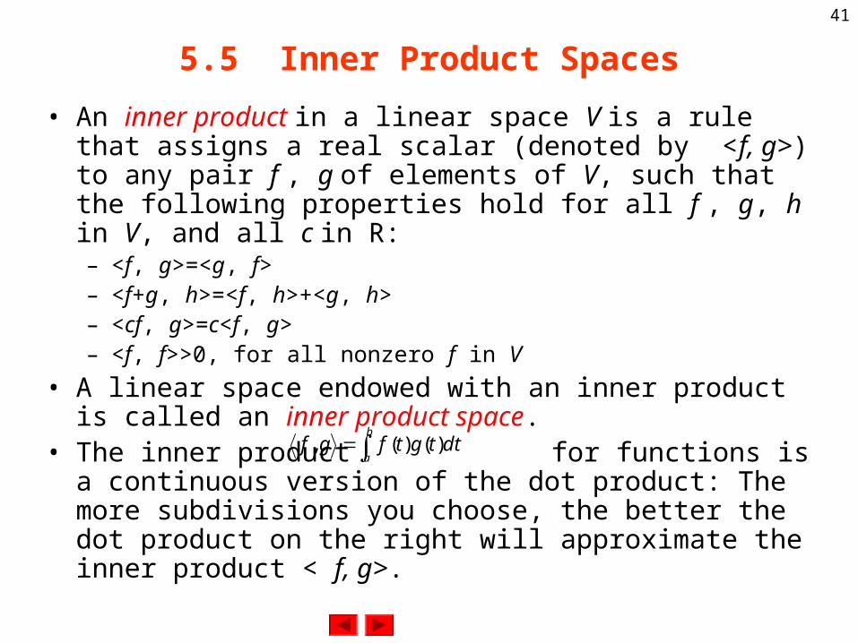
5.5 Inner Product Spaces

• An inner product in a linear space V is a rule that assigns a real scalar (denoted by <f, g>) to any pair f , g of elements of V, such that the following properties hold for all f , g, h in V, and all c in R:– <f, g>=<g, f>– <f+g, h>=<f, h>+<g, h>– <cf, g>=c<f, g>– <f, f>>0, for all nonzero f in V

• A linear space endowed with an inner product is called an inner product space.

• The inner product for functions is a continuous version of the dot product: The more subdivisions you choose, the better the dot product on the right will approximate the inner product < f, g>.

b

adttgtfgf )()(,

42

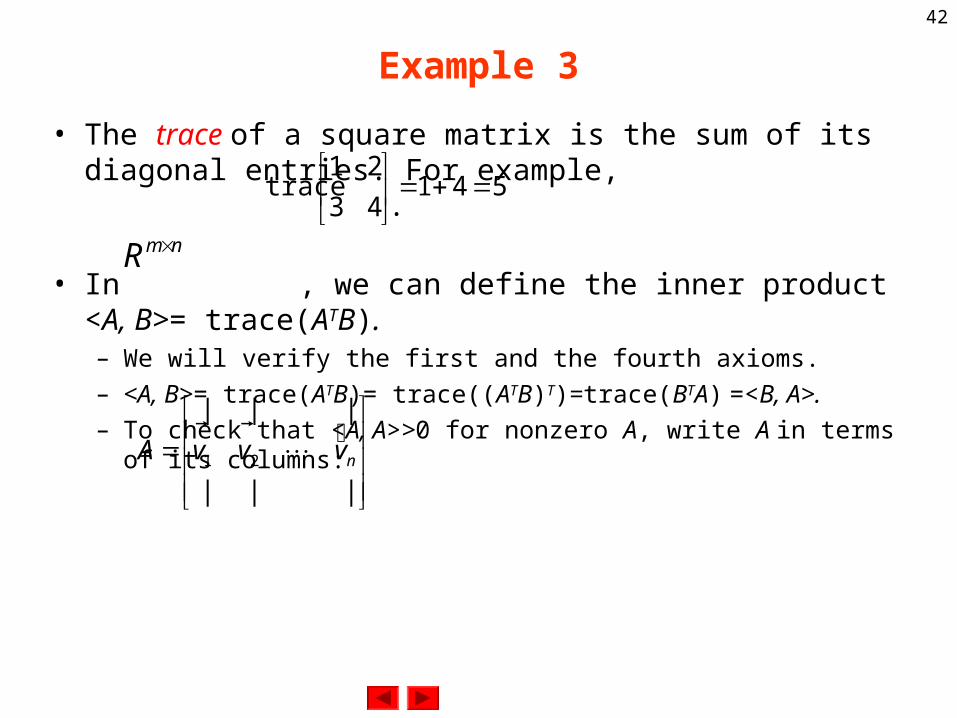
Example 3

• The trace of a square matrix is the sum of its diagonal entries. For example, .

• In , we can define the inner product <A, B>= trace(ATB).– We will verify the first and the fourth axioms.

– <A, B>= trace(ATB)= trace((ATB)T)=trace(BTA) =<B, A>.

– To check that <A, A>>0 for nonzero A, write A in terms of its columns:

54143

21trace

nmR

|||

|||

21 nvvvA%

43

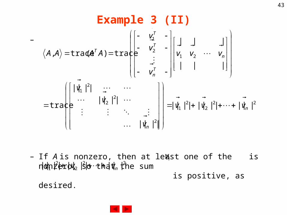
Example 3 (II)

–

– If A is nonzero, then at least one of the is nonzero, so that the sum is positive, as desired.

222

21

2

22

21

212

1

||||||||||||

||||

||||

||||

trace

|||

|||

trace)(trace,

n

n

n

Tn

T

T

T

vvv

v

v

v

vvv

v

v

v

AAAA

222

21 |||||||||||| nvvv

iv

44

Norm, orthogonality

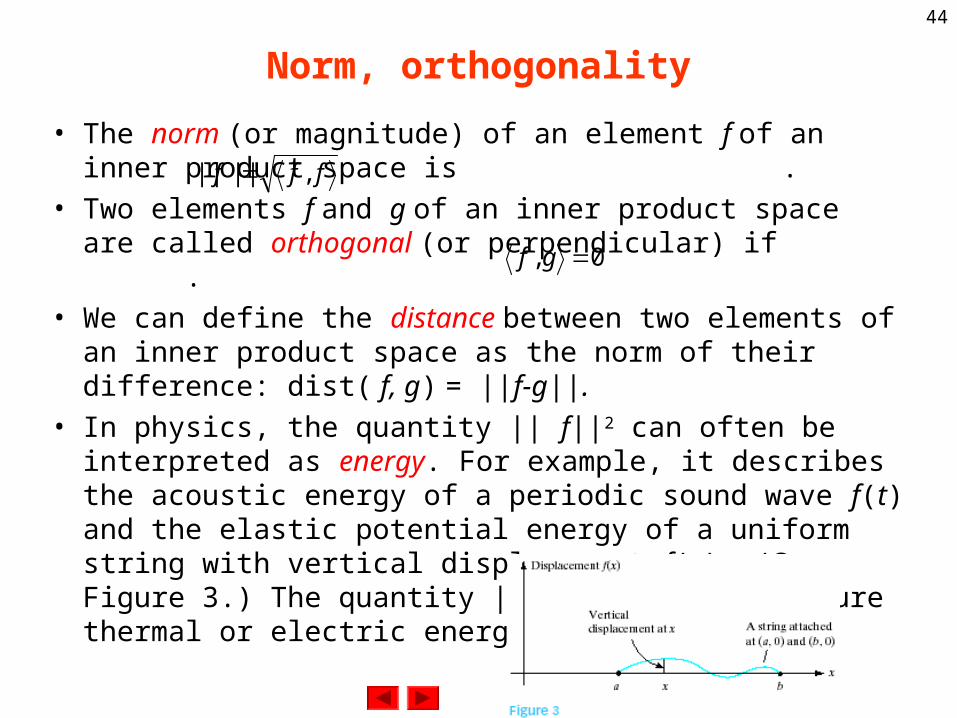
• The norm (or magnitude) of an element f of an inner product space is .

• Two elements f and g of an inner product space are called orthogonal (or perpendicular) if .

• We can define the distance between two elements of an inner product space as the norm of their difference: dist( f, g) = ||f-g||.

• In physics, the quantity || f||2 can often be interpreted as energy. For example, it describes the acoustic energy of a periodic sound wave f(t) and the elastic potential energy of a uniform string with vertical displacement f(x). (See Figure 3.) The quantity || f||2 may also measure thermal or electric energy.

fff ,||||

0, gf

45

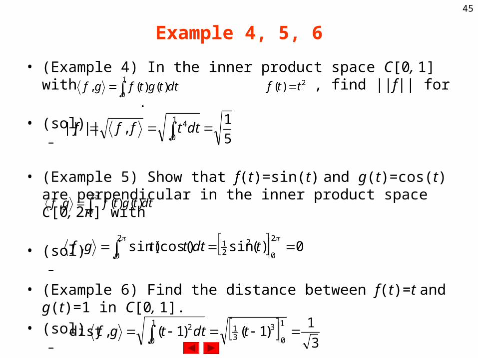
Example 4, 5, 6

• (Example 4) In the inner product space C[0, 1] with , find ||f|| for .

• (sol)–

• (Example 5) Show that f(t)=sin(t) and g(t)=cos(t) are perpendicular in the inner product space C[0, 2π] with

• (sol)–

• (Example 6) Find the distance between f(t)=t and g(t)=1 in C[0, 1].

• (sol)–

1

0)()(, dttgtfgf 2)( ttf

5

1,||||

1

0

4 dttfff

2

0)()(, dttgtfgf

2

0

2

0

221 0)(sin)cos()sin(, tdtttgf

3

1)1()1(,dist

1

0

331

1

0

2 tdttgf

46

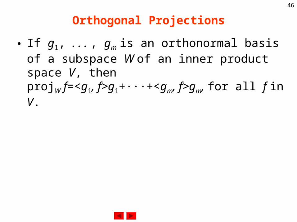
Orthogonal Projections

• If g1, . . . , gm is an orthonormal basis of a subspace W of an inner product space V, thenprojW f=<g1, f>g1+···+<gm, f>gm, for all f in V.

47

Example 7

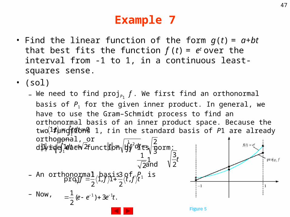
• Find the linear function of the form g(t) = a+bt that best fits the function f (t) = et over the interval from -1 to 1, in a continuous least-squares sense.

• (sol)– We need to find projP1

f . We first find an orthonormal basis of P1 for the

given inner product. In general, we have to use the Gram–Schmidt process to find an orthonormal basis of an inner product space. Because the two functions 1, t in the standard basis of P1 are already orthogonal, or , we merely need to divide each function by its norm:

and

– An orthonormal basis of P1 is and

– Now,

0,11

1 tdtt

2111

1 dt

3

21

1

2 dttt

12

1 t2

3

.3)(2

1

,2

31,1

2

1proj

11

1

teee

tftffP

48

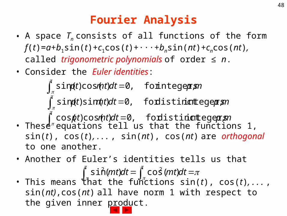
Fourier Analysis• A space Tn consists of all functions of the form

f(t)=a+b1sin(t)+c1cos(t)+···+bnsin(nt)+cncos(nt),called trigonometric polynomials of order ≤ n.

• Consider the Euler identities:

• These equations tell us that the functions 1, sin(t), cos(t), . . . , sin(nt), cos(nt) are orthogonal to one another.

• Another of Euler’s identities tells us that

• This means that the functions sin(t), cos(t), . . . , sin(nt),cos(nt) all have norm 1 with respect to the given inner product.

mpdtmtpt , integersfor ,0)cos()sin(

mpdtmtpt , integersdistinct for ,0)sin()sin(

mpdtmtpt , integersdistinct for ,0)cos()cos(

dtmtdtmt )(cos)(sin 22

49

Orthonormal Basis in Fourier Analysis

• Let Tn be the space of all trigonometric polynomials of order ≤n, with the inner product

then, the function

form an orthonormal basis of Tn.

dttgtfgf )()(

1,

)cos(),sin(,),2cos(),2sin(),cos(),sin(,2

1ntnttttt

50

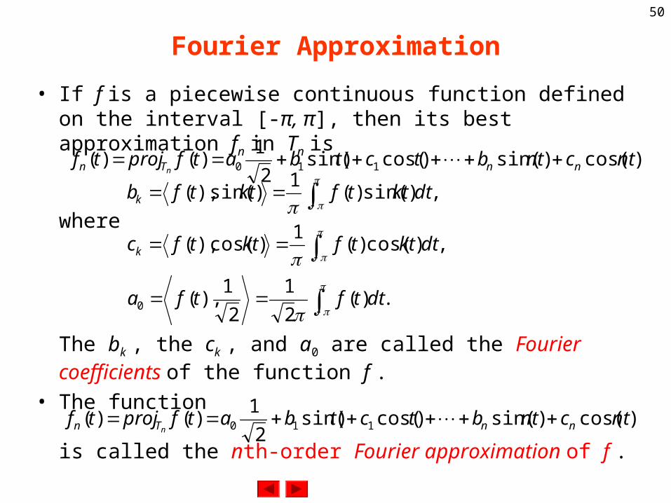
Fourier Approximation

• If f is a piecewise continuous function defined on the interval [-π, π], then its best approximation fn in Tn is

where

The bk , the ck , and a0 are called the Fourier coefficients of the function f .

• The function

is called the nth-order Fourier approximation of f .

),cos()sin()cos()sin(2

1)()( 110 ntcntbtctbatfprojtf nnTn n

.)(2

1

2

1),(

,)cos()(1

)cos(),(

,)sin()(1

)sin(),(

0 dttftfa

dtkttfkttfc

dtkttfkttfb

k

k

),cos()sin()cos()sin(2

1)()( 110 ntcntbtctbatfprojtf nnTn n

51

Example 8

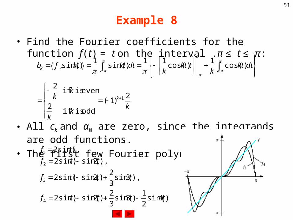
• Find the Fourier coefficients for the function f(t) = t on the interval .π ≤ t ≤ π:

• All ck and a0 are zero, since the integrands are odd functions.

• The first few Fourier polynomials are

kk

k

kk

dtktk

tktk

dtktktfb

k

k

2)1(

odd is if 2

even is if 2

)cos(1

)cos(11

)sin(1

)sin(,

1

)4sin(2

1)3sin(

3

2)2sin()sin(2

),3sin(3

2)2sin()sin(2

),2sin()sin(2

),sin(2

4

3

2

1

ttttf

tttf

ttf

tf

52

Fourier Analysis (II)

• The infinite series of the squares of the Fourier coefficients of a piecewise continuous function f converges to ||f||2.

22221

21

20 |||| fcbcba nn