Embed Size (px)
Citation preview
Second-Order Draft Chapter 8 IPCC WG1 Fourth Assessment Report
1 2 3 4 5 6 7 8 9
10 11 12 13 14 15 16 17 18 19 20 21 22 23 24 25 26 27 28 29
Chapter 8: Climate Models and Their Evaluation
Coordinating Lead Authors: David Randall (USA), Richard A. Wood (UK) Lead Authors: Sandrine Bony (France), Robert Colman (Australia), Thierry Fichefet (Belgium), John Fyfe (Canada), Vladimir Kattsov (Russia), Andrew Pitman (Australia), Jagadish Shukla (USA), Jayaraman Srinivasan (India), Ronald J. Stouffer (USA), Akimasa Sumi (Japan), Karl Taylor (USA) Contributing Authors: K. Achuta Rao (USA), R. Allan (UK), A. Berger (Belgium), H. Blatter, C. Bonfils (USA), A. Boone (France), C. Bretherton (USA), T. Broccoli (USA), V. Brovkin (Germany), W. Cai (Australia), M. Claussen (Germany), P. Dirmeyer (USA), C. Doutriaux (USA), H. Drange (Norway), J.-L. Dufresne (France), S. Emori (Japan), A. Frei (USA), A. Ganopolski (Germany), P. Gent (USA), P. Gleckler (USA), H. Goosse (Belgium), R. Graham (UK), J. Gregory (UK), R. Gudgel (USA), A. Hall (USA), S. Hallegatte (France), H. Hasumi (Japan), A. Henderson-Sellers, H. Hendon (Australia), K. Hodges (UK), M. Holland (USA), A.A.M.. Holtslag (The Netherlands), E. Hunke (USA), P. Huybrechts (Belgium), W. Ingram (UK), F. Joos (Switzerland), B. Kirtman (USA), S. Klein (USA), R. Koster (USA), P. Kushner (Canada), J. Lanzante (USA), M. Latif (Germany), G. Lau (USA), M. Meinshausen (USA), A.H. Monahan (Canada), J. Murphy (UK), T. Osborn (UK), T. Pavlova (Russia), V. Petoukhov(Germany), T. Phillips (USA), S. Power (Australia), S. Rahmstorf (Germany), S. Raper (UK), H. Renssen (The Netherlands), D. Rind (USA), M. Roberts (UK), A. Rosati (USA), C. Schär (Switzerland), J. Scinnoca (Canada), A. Schmittner (USA), D. Seidov (USA), A.G. Slater (USA), D. Smith (UK), B. Soden (USA), W. Stern (USA), D. Stone (UK), K.Sudo (Japan), G. Tselioudis (USA), M. Webb (UK), M. Wild (Switzerland), T.Yakemura (Japan). Review Editors: Elisa Manzini (Italy), Taroh Matsuno (Japan), Bryant McAvaney (Australia) Date of Draft: 3 March 2006 Notes: TSU compiled version
30 31 32 33 34 35 36 37 38 39 40 41 42 43 44 45 46 47 48 49 50 51 52 53 54 55 56 57 58 59
Table of Contents Executive Summary............................................................................................................................................................3 8.1 Introduction and Overview ........................................................................................................................................7
8.1.1 What is Meant by Evaluation? ......................................................................................................................7 8.1.2 Methods of Evaluation ..................................................................................................................................7 8.1.3 How Are Models Constructed? .....................................................................................................................9
8.2 Advances in Modelling............................................................................................................................................10 8.2.1 Atmospheric Processes ...............................................................................................................................10 8.2.2 Ocean Processes .........................................................................................................................................12 8.2.3 Terrestrial Processes ..................................................................................................................................14 8.2.4 Cryospheric Processes................................................................................................................................15 8.2.5 Aerosol Modelling and Atmospheric Chemistry .........................................................................................16 8.2.6 Coupling Advances .....................................................................................................................................17 8.2.7 Flux Adjustments and Initialization ............................................................................................................17
8.3 Evaluation of Contemporary Climate as Simulated by Coupled Global Models.....................................................18 8.3.1 Atmospheric Component .............................................................................................................................19 8.3.2 Ocean Component Evaluation ....................................................................................................................23 8.3.3 Sea Ice.........................................................................................................................................................26 8.3.4 Land-Surface Component ...........................................................................................................................27 8.3.5 Tracking Changes in Model Performance ..................................................................................................28
8.4 Evaluation of Large-Scale Climate Variability as Simulated by Coupled Global Models ......................................29 8.4.1 Northern and Southern Annular Modes (NAM and SAM) ..........................................................................29 8.4.2 Pacific Decadal Variability ........................................................................................................................31 8.4.3 Pacific-North American (PNA) Pattern ......................................................................................................32 8.4.4 Cold Ocean-Warm Land (COWL) Pattern..................................................................................................33 8.4.5 Atmospheric Regimes and Blocking............................................................................................................33 8.4.6 Atlantic Multidecadal Variability ...............................................................................................................34
Do Not Cite or Quote 8-1 Total pages: 99
Second-Order Draft Chapter 8 IPCC WG1 Fourth Assessment Report
1 2 3 4 5 6 7 8 9
10 11 12 13 14 15 16 17 18 19 20 21 22 23 24 25 26 27 28
8.4.7 El Niño-Southern Oscillation (ENSO) ........................................................................................................34 8.4.8 Madden-Julian Oscillation (MJO).............................................................................................................35 8.4.9 Quasi-Biennial Oscillation (QBO).............................................................................................................36 8.4.10 Monsoon Variability...................................................................................................................................37 8.4.11 Predictions Using “IPCC” Models.............................................................................................................37
8.5 Model Simulations of Extremes ..............................................................................................................................38 8.5.1 Extreme Temperature..................................................................................................................................39 8.5.2 Extreme Precipitation .................................................................................................................................39 8.5.3 Tropical Cyclones .......................................................................................................................................40 8.5.4 Summary .....................................................................................................................................................41
8.6 Climate Sensitivity and Feedbacks ..........................................................................................................................41 8.6.1 Introduction ................................................................................................................................................41 8.6.2 Interpretation of the Range of Climate Sensitivity Estimates Among GCMs. .............................................41 8.6.3 Key Physical Processes Involved in Climate Sensitivity .............................................................................43
Box 8.1 Upper Tropospheric Humidity and Water Vapour Feedback ........................................................................46 8.6.4 How to Assess Our Relative Confidence in the Feedbacks Simulated by the Different Models?................52
8.7 Mechanisms Producing Thresholds and Abrupt Climate Change ...........................................................................52 8.7.1 Introduction ................................................................................................................................................52 8.7.2 Forced Response.........................................................................................................................................53 8.7.3 Unforced Abrupt Climate Change ..............................................................................................................56
8.8 Representing the Global System with Simpler Models ...........................................................................................56 8.8.1 Why Lower Complexity? .............................................................................................................................56 8.8.2 Simple Climate Models ..............................................................................................................................57 8.8.3 Earth System Models of Intermediate Complexity ......................................................................................58
References ........................................................................................................................................................................60 Question 8.1: How Reliable Are the Models Used to Make Projections of Future Climate Change?..............................91 Tables ...............................................................................................................................................................................93
Do Not Cite or Quote 8-2 Total pages: 99
Second-Order Draft Chapter 8 IPCC WG1 Fourth Assessment Report
1 2 3 4 5 6 7 8 9
10 11 12 13 14 15 16 17 18 19 20 21 22 23 24 25 26 27 28 29 30 31 32 33 34 35 36 37 38 39 40 41 42 43 44 45 46 47 48 49 50 51 52 53 54 55 56
Executive Summary This chapter assesses the capacity of the global climate models used elsewhere in this report for projecting future climate change. Confidence in model estimates of future climate evolution has been enhanced via a range of advances since the TAR. There is considerable confidence that climate models provide plausible quantitative estimates of future climate change, particularly at continental scales and above. Confidence in these estimates is higher for some climate variables (e.g. temperature) than for others (e.g. precipitation). This confidence comes from the foundation of the models in accepted physical principles and from their ability to reproduce observed features of recent climate (see Chapters 8, 9) and past climate changes (see Chapter 6). In this summary we highlight areas of progress since the TAR:
• There have been ongoing improvements to resolution, numerics and parametrisations, and additional processes (e.g., interactive aerosols) have been included in more of the models.
• Few models continue to use flux adjustments which were previously required to maintain a stable climate. The uncertainty associated with the use of those adjustments is therefore decreasing, although biases and long term trends remain in AOGCM control simulations.
• There have been improvements in the simulation of many aspects of present climate despite the fact that flux adjustments have been eliminated in most models.
• Progress in the simulation of important modes of climate variability has increased our overall confidence in the models’ representation of important climate processes. Some problems remain in the simulation of ENSO (despite an overall improvement), and for other modes of variability, notably the MJO.
• The ability of models to simulate extreme events, especially hot and cold spells, has improved, but simulation of extreme precipitation remains variable, with generally too little precipitation falling in the most intense events.
• Simulation of extratropical cyclones has improved. Some models can simulate the large scale conditions necessary to infer the frequency and distribution of tropical cyclones.
• Substantial progress has been made in understanding the differences in equilibrium climate sensitivity found in different models. Cloud feedbacks have been confirmed as a primary source of inter-model differences, with low cloud the largest contributor. New observational and modelling evidence strongly supports a combined water vapour-lapse rate feedback of a strength comparable to that found in GCMs. The magnitude of cryospheric feedbacks remains uncertain, contributing particularly to the range of model climate responses at mid-to-high latitudes.
• Systematic biases have been found in most models’ simulation of the Southern Ocean. Since the Southern Ocean is important for ocean heat uptake this results in some uncertainty in transient climate response.
• The possibility that metrics based on historical observations might be used to constrain model projections of climate change has been explored for the first time through the analysis of large ensembles of simulations by closely related models. Nevertheless, a proven set of model metrics that might be used to narrow the range of plausible climate projections has yet to be developed.
• Models are increasingly being subjected to a more comprehensive set of diagnostic tests, including tests of their ability to forecast on time scales from days to a year, when initialized with observed conditions. The more diverse set of tests increases confidence in the fidelity with which models represent processes that impact climate projections.
• In order to explore the potential importance of carbon cycle feedbacks in the climate system, explicit treatment of the carbon cycle has been introduced in a few climate AOGCMs and some Earth System Models of Intermediate Complexity (EMICs).
• EMICs have been evaluated in greater depth than previously. Intercomparison exercises have demonstrated that these models are very useful to study questions involving long timescales or requiring a large number of ensemble simulations or sensitivity experiments.
• Enhanced scrutiny of models and expanded diagnostic analysis of model behavior has been increasingly facilitated by internationally coordinated efforts to collect and disseminate output from model experiments performed under common conditions. This has encouraged a more comprehensive and open evaluation of models. The expanded evaluation effort, encompassing a diversity of
Do Not Cite or Quote 8-3 Total pages: 99

Second-Order Draft Chapter 8 IPCC WG1 Fourth Assessment Report
1 2 3 4 5 6 7 8 9
10 11 12 13 14 15 16 17 18 19 20 21 22 23 24 25 26 27 28 29 30 31 32 33 34 35 36 37 38 39 40 41 42 43 44 45 46 47 48 49 50 51 52 53 54 55 56
perspectives, makes it less likely that significant model errors are being overlooked. Developments in model formulation Improvements in atmospheric models include reformulated dynamics and transport schemes, and increased horizontal and vertical resolution. Interactive aerosol modules have been incorporated into some models, and through these, the direct and the indirect effect of aerosols are now more widely included Significant developments have occurred in the representation of terrestrial processes. Individual components continue to be improved via a systematic evaluation against observations and against more comprehensive models. The terrestrial processes that might significantly affect large-scale climate over the next few decades are included in current climate models. Development of the oceanic component of AOGCMs has continued. Resolution has increased and models have generally abandoned the so-called "rigid lid" treatment of the ocean surface. New physical parameterizations and numerics include true freshwater fluxes, improved river and estuary mixing schemes, and the use of positive definite advection schemes. Adiabatic isopycnal mixing schemes are now widely used. Some of these improvements have led to a reduction in the uncertainty associated with the use of less sophisticated parameterizations (e.g. virtual salt flux). Progress in developing AOGCM cryospheric components is clearest for sea ice. Almost all state-of-the-art AOGCMs now include more elaborate sea-ice dynamics and some now include several sea-ice thickness categories and relatively advanced thermodynamics. AOGCM parameterizations of terrestrial snow processes vary considerably in formulation. Systematic evaluation of snow suggests that surface tiling and sub-grid scale heterogeneity are important for simulating observations of seasonal snow cover. Few AOGCMs include ice sheet dynamics, and in all of the AOGCMs evaluated in this chapter and used in Chapter 10 for projecting climate change in the 21st Century, the permanent ice cover is prescribed. Developments in model climate simulation Although tracking changes in overall coupled model performance is still difficult, there is some evidence, based on experiments in which atmospheric GCMs are run with prescribed ocean and sea ice conditions, that the large-scale seasonal variations in a number of climatologically important fields are better simulated now than they were a decade ago. Simulation of marine low-level clouds, which are important for correctly simulating sea surface temperature and cloud feedback in a changing climate, has improved in some models. Nevertheless, errors in cloud simulation remain in many models. Some common model biases in the Southern Ocean have been identified, resulting in some uncertainty in heat uptake and transient climate response. Simulation of the thermocline, which was too thick, and the Atlantic overturning and heat transport, which were both too weak in earlier models, has been substantially improved in many models. It is likely that at least part of the improvement is due to the improvements in formulation mentioned above. Despite notable progress in developing AOGCM sea ice components, and an improved ability of some models to capture key features of sea-ice distribution and seasonality, AOGCMs have typically demonstrated only modest improvement in simulations of observed sea-ice since the TAR. The relatively slow progress can partially be explained by the fact that improving sea ice simulation requires improvements in both the atmosphere and ocean components in addition to the sea ice component itself. Since the TAR, developments in AOGCM formulation have improved the representation of large-scale variability over a wide range of time-scales. The models capture the dominant extratropical patterns of variability including the Northern and Southern Annular Modes, the Pacific Decadal Oscillation, the Pacific-North American and Cold Ocean-Warm Land Patterns. AOGCMs simulate Atlantic multidecadal variability, although the relative roles of high and low latitude processes appear to differ between models. In the tropics, there has been an overall improvement in the AOGCM simulation of the spatial pattern and frequency of the El Niño – Southern Oscillation, but problems remain in simulating its seasonal phase locking and the
Do Not Cite or Quote 8-4 Total pages: 99
Second-Order Draft Chapter 8 IPCC WG1 Fourth Assessment Report
1 2 3 4 5 6 7 8 9
10 11 12 13 14 15 16 17 18 19 20 21 22 23 24 25 26 27 28 29 30 31 32 33 34 35 36 37 38 39 40 41 42 43 44 45 46 47 48 49 50 51 52 53 54 55 56 57
asymmetry between El Niño and La Niña episodes. Variability with characteristics of the Madden-Julian Oscillation is simulated in most AOGCMs, but typically too infrequently and with insufficient strength. GCMs are able to simulate extreme warm temperatures, cold air outbreaks and frost days reasonably well. Despite resolutions that are too coarse to resolve tropical cyclones, some coupled climate models can simulate the statistics of the larger-scale conditions necessary for tropical cyclone genesis. Simulation of extreme precipitation is dependent on resolution, parametrization and the thresholds chosen. In general models tend to produce too many days with weak precipitation (<10 mm day–1) and too little precipitation overall in intense events (>10 mm day–1). Given the large computing resources required by AOGCMs, Earth system models of intermediate complexity (EMICs) are widely used to study issues in past and future climate change that cannot be addressed with AOGCMs. Because of the reduced resolution of EMICs and their simplified representation of some physical processes, these models only allow inferences about very large scales. Since the TAR, EMICs have been evaluated via organised model intercomparisons which have revealed that, at large scales, EMIC results can compare well with observational data and AOGCM results. This lends support to the view that EMICS can be used to gain understanding of processes and interactions within the climate system that evolve on time-scales beyond those generally accessible to GCMs. The uncertainties in long-term climate change projections can also be explored more comprehensively by using large ensembles of EMIC runs. Developments in analysis methods Since the TAR, an unprecedented effort has been initiated to make available new model results for scrutiny by scientists outside the modelling centers. Sixteen modeling groups performed a set of coordinated, standard experiments, and the resulting model output, analyzed by hundreds of researchers worldwide, forms the basis for much of the current IPCC assessment of model results. The benefits of coordinated model intercomparison include increased communication among modelling groups, more rapid identification and correction of errors, the creation of standardized benchmark calculations, and a more complete and systematic record of modelling progress. A few climate models have been tested for (and shown) skill in initial value predictions, on timescales from weather forecasting (a few days) to seasonal forecasting (annual). The skill demonstrated by models under these conditions increases confidence that they simulate some of the key processes and teleconnections in the climate system. Developments in evaluation of climate feedbacks Water vapour feedback remains the most important positive feedback in modelled climate sensitivity. Although the strength of this feedback varies among models, its overall impact on the spread of model climate sensitivities is reduced by lapse rate feedback, which tends to be anticorrelated. Several new studies indicate that modelled lower and upper tropospheric relative humidity respond to seasonal and interannual variability, volcanic induced cooling and climate trends, in a way consistent with observations. Taken together, observational and modelling evidence strongly favour a combined water vapour-lapse rate feedback of around the strength found in AOGCMs. Recent studies reaffirm that the spread of climate sensitivity estimates among models arises primarily from inter-model differences in cloud feedbacks. The shortwave impact of changes in boundary-layer clouds, and to a lesser extent mid-level clouds, constitutes the largest contributor to inter-model differences in global cloud feedbacks. The relatively poor simulation of these clouds in the present climate is a reason for some concern. The response to global warming of deep convective clouds is also a significant source of uncertainty in projections since current models predict different responses of these clouds. Observationally-based evaluation of cloud feedbacks indicate that climate models exhibit different strengths and weaknesses, and it is not yet possible to determine which estimates of the climate change cloud feedbacks are the most reliable. Despite advances since the TAR, substantial uncertainty remains in the magnitude of cryospheric feedbacks within AOGCMs. This contributes to a spread of modelled climate response, particularly in high latitudes,
Do Not Cite or Quote 8-5 Total pages: 99

Second-Order Draft Chapter 8 IPCC WG1 Fourth Assessment Report
1 2 3 4 5 6 7 8 9
10 11 12 13 14 15 16 17 18 19
although there is growing evidence that cryospheric feedbacks are only partly responsible for polar amplification. On the global scale, the surface albedo feedback is positive in all the models, with a spread among current models much smaller than that of cloud feedbacks. Understanding and evaluating sea-ice feedbacks is complicated by the strong coupling to polar cloud processes and ocean heat and freshwater transport. Scarcity of observations in polar regions also hampers evaluation. New techniques that estimate sea-ice and land-snow albedo feedbacks have recently been developed. Model performance in reproducing the observed seasonal cycle of land snow cover may provide an indirect evaluation of the simulated snow-albedo feedback. Systematic model comparisons have helped establish the key processes responsible for differences among models in the response of the ocean to climate change (especially ocean heat uptake and thermohaline circulation changes). The importance of feedbacks from surface flux changes on the meridional overturning circulation has been established in many models. At present, these feedbacks are not tightly constrained by available observations. The approach discussed above for analyzing processes contributing to model feedbacks, together with recent studies based on large ensembles of models, suggests that in the future it may be possible to use observations to narrow the current spread in model projections of climate change.
Do Not Cite or Quote 8-6 Total pages: 99
Second-Order Draft Chapter 8 IPCC WG1 Fourth Assessment Report
1 2 3 4 5 6 7 8 9
10 11 12 13 14 15 16 17 18 19 20 21 22 23 24 25 26 27 28 29 30 31 32 33 34 35 36 37 38 39 40 41 42 43 44 45 46 47 48 49 50 51 52 53 54 55 56
8.1 Introduction and Overview The goal of this chapter is to evaluate the capabilities and limitations of the global climate models used elsewhere in this assessment. A number of model evaluation activities are described in various chapters of this report. This section provides a context for those studies and a guide to direct the reader to the appropriate chapters. 8.1.1 What is Meant by Evaluation? A specific prediction based on a model can often be demonstrated to be right or wrong, but the model itself should always be viewed critically. This is true for both weather prediction and climate prediction. Weather forecasts are produced on a regular basis, and can be quickly tested against what actually happened. Over time, statistics can be accumulated that give information on the performance of a particular model or forecast system. In climate change simulations, on the other hand, we use models to make projections of possible future changes, for which timescales are many decades and for which there are no precise past analogues. We can gain confidence in a model through simulations of the historical record, or of paleoclimate, but such opportunities are much more limited than those available through weather prediction. These and other approaches are discussed below. 8.1.2 Methods of Evaluation A climate model is a very complex system, with many components. The model must of course be tested at the system level, i.e., by running the full model and comparing the results with observations. Such tests can reveal problems, but their source is often hidden by the model's complexity. For this reason, it is also important to test the model at the component level, i.e., by isolating particular components and testing them independent of the complete model. Component-level evaluation of climate models is common. Numerical methods are tested in standardized tests, organized through activities such as the quasi-biennial Workshops on Partial Differential Equations on the Sphere. Physical parameterizations used in climate models are being tested through numerous case studies (some based on observations and some idealized), organized through programs such as ARM, EUROCS, and GCSS. These various activities have been ongoing for a decade or more. A large body of results has been published (e.g., Randall et al., 2003). System-level evaluation is focused on the outputs of the full model, i.e., model simulations of particular observed climate variables. Studies can be divided into three categories: simulation of the present climate (Chapter 8), simulation of the instrumental record (see Chapter 9), and simulation of paleo-climate (see Chapter 6). Testing models’ ability to simulate ‘present climate’ (including variability and extremes) is an important part of model evaluation (see Sections 8.3 to 8.5). In doing this, certain practical choices are needed, e.g. between a long timeseries or mean from a ‘control’ run with fixed radiative forcing (often preindustrial rather than present day), or a shorter, transient timeseries from a ‘20th-century’ simulation including historical variations in forcing. Such decisions are made by individual researchers, dependent on the particular problem being studied. Differences between model and observations should be considered insignificant if they are within
1. unpredictable internal variability (e.g., the observational period contained an unusual number of El Niño events)
2. expected differences in forcing (e.g., observations for the 1990s compared with a ‘preindustrial’ model control run)
3. uncertainties in the observed fields and while space does not allow a discussion of the above issues in detail for each climate variable, they are taken into account in the overall evaluation.
Do Not Cite or Quote 8-7 Total pages: 99
Second-Order Draft Chapter 8 IPCC WG1 Fourth Assessment Report
1 2 3 4 5 6 7 8 9
10 11 12 13 14 15 16 17 18 19 20 21 22 23 24 25 26 27 28 29 30 31 32 33 34 35 36 37 38 39 40 41 42 43 44 45 46 47 48 49 50 51 52 53 54 55 56 57
What does the accuracy of a model’s simulation of contemporary mean climate tell us about the accuracy of its projections of climate change? A full answer to this question remains elusive, but two approaches are possible. The first is to use an analysis of the mechanisms generating climate change in model simulations (e.g., Sections 8.6, 8.7) to provide insight into which aspects of the ‘mean climate state’ are important. For example analysis of the sea ice – albedo feedback (see Section 8.6.3.3) suggests that accurate simulation of mean sea ice fields may be of moderate importance for global climate sensitivity, and considerable importance for high latitude sensitivity (Holland and Bitz, 2003). The second approach is to use the emerging multi-model or ‘perturbed physics’ ensembles to make a ‘perfect model’ study of sensitivity of climate response to particular observational constraints. For example Murphy et al. (2004), Knutti et al. (2006), Piani et al. (2005), and Shukla et al. (2006) show that using specific observational constraints to weight members in a perturbed physics ensemble gives tighter constraints on the ensemble distribution of climate sensitivity than if the observations are not used. On the other hand Hargreaves et al. (2004) generate an ensemble of Earth System Models of Intermediate Complexity (EMICs) that all give good simulations of present-day mean ocean temperature and salinity and atmospheric surface temperature and humidity, but find that these observational constraints alone do not give a strong constraint on the future behaviour of the ocean thermohaline circulation. All the above studies are subject to two restrictions: (i) they are dependent on the structure of the particular model or ensemble used, so conclusions may be misleading if a key process or feedback is absent in all the driving models, (ii) a prior choice of observational constraints is required, and this may to a large extent be subjective. Therefore we are some way from a robust ‘model metric’ for likelihood weighting of different models; but these results do suggest that the observational tests currently available do have value in constraining climate projections. Further useful constraints come from models’ ability to simulate past climate (see Chapters 6 and 9). Models have been extensively used to simulate observed climate change during the 20th century. Since radiative forcing is not perfectly known over that period (see Chapter 2), such tests do not fully constrain future reponse to forcing changes. Knutti et al. (2002) show that in a perturbed physics EMIC ensemble, models with a range of climate sensitivities are consistent with the observed surface air temperature and ocean heat content records, if aerosol forcing is allowed to vary within its range of uncertainty. Despite this fundamental limitation, testing of 20th century simulations against historical observations does place some constraints on future climate response (e.g., Knutti et al. 2002). These topics are discussed in detail in Chapter 9. Simulations of past climate states allow models to be exercised in regimes that are significantly different from the present. Such tests complement the ‘present climate’ and ‘instrumental period climate’ evaluations, since 20th Century climate variations have been small compared with the anticipated future changes under SRES forcing scenarios. The limitations of palaeoclimate tests are that uncertainties in both forcing and actual climate variables (usually derived from proxies) tend to be greater than in the instrumental period. Further, climate states may have been so different (e.g., ice sheets at last glacial maximum) that processes determining quantities such as climate sensitivity were different from those likely to operate in the 21st Century. Finally, the timescales of change were so long that there are difficulties in experimental design, at least for GCMs. These issues are discussed in depth in Chapter 6. Climate models can be tested through forecasts based on initial conditions. Climate models are closely related to the models that are used routinely for numerical weather prediction (NWP), and increasingly for extended range forecasting on seasonal to interannual timescales. Typically, however, models used for NWP are run at higher resolution than is possible for climate. Evaluation of such forecasts tests the models’ representation of some key processes in the atmosphere and ocean, although the links between these processes and long-term climate response have not always been established. It must be remembered that the quality of an initial value prediction is dependent on several factors beyond the numerical model itself (e.g., data assimilation techniques, ensemble generation method), and these factors may be less relevant to projecting the long term, forced response of the climate system to changes in radiative forcing. There is a large literature on this topic, but to maintain focus on the goal of this chapter we confine ourselves to the relatively few studies that have been conducted using models that are very closely related to the climate models used for projections (see Section 8.4.11). Finally, we note that over thirty years ago climate models predicted that an increase in atmospheric CO2 would lead to a warming of the troposphere, especially in the polar regions, an increase in the speed of the
Do Not Cite or Quote 8-8 Total pages: 99
Second-Order Draft Chapter 8 IPCC WG1 Fourth Assessment Report
hydrologic cycle, and a cooling of the stratosphere (e.g., Manabe and Wetherald, 1975). As discussed elsewhere in this Assessment, each of these changes has since been observed. Over these 30 years, while climate models have evolved greatly, their projections of the impact of increasing CO
1 2 3 4 5 6 7 8 9
10 11 12 13 14 15 16 17 18 19 20 21 22 23 24 25 26 27 28 29 30 31 32 33 34 35 36 37 38 39 40 41 42 43 44 45 46 47 48 49 50 51 52 53 54 55 56 57
2 have remained remarkably unchanged, and these projections are consistent with the growing observational record. 8.1.2.1 Evaluation of climate change mechanisms and feedbacks The component-level and system-level methods of evaluation provide complementary perspectives on models. One way to bring together these two levels of evaluation is to base evaluation on an analysis of those mechanisms that are believed to control climate change response (e.g. Sections 8.6, 8.7). The impact of system-level and component-level errors can then be assessed against their likely impacts on the key mechanisms. 8.1.2.2 Model intercomparisons The global model intercomparison activities that began in the late 1980s (e.g., Cess et al., 1989), and continued with AMIP (the Atmosphere Model Intercomparison Project), have now proliferated to include several dozen “MIPs”, covering virtually all climate model components and various coupled model configurations. A summary is available at http://www.ifm.uni-kiel.de/other/clivar/science/mips.htm. By far the most ambitious organized effort to collect and analyze coupled model output from standardized experiments was undertaken in the last few years (see http://www-pcmdi.llnl.gov/ipcc/about_ipcc.php). It differed from previous model intercomparisons in that a more complete set of experiments was performed, including unforced control simulations, simulations attempting to reproduce historically observed climate change, and simulations of future climate change. It also differed in that multiple simulations were performed by individual models to make it easier to separate climate change signals from “noise” (i.e., unforced variability within the climate system). Perhaps the most important change from earlier efforts was the collection of a more comprehensive set of model output. This allowed hundreds of researchers from outside the modeling groups to scruitinize the models from a variety of perspectives. Th enhancement in diagnostic analysis of climate model results represents an important step forward since the TAR. Overall, the vigorous, ongoing intercomparison activities have increased communication among modelling groups, allowed rapid identification and correction of modeling errors, and encouraged the creation of standardized benchmark calculations, as well as a more complete and systematic record of modelling progress. A downside is that the effort required of modeling groups to run standardized experiments, prepare output for use by others, and provide model documentation to the community at large impinges on the groups’ own research agendas. There is recognition that model intercomparison activities and standardized experiments should not “crowd out” other creative research, but some disagreement concerning how resources should be apportioned among them. 8.1.3 How Are Models Constructed? The fundamental basis on which climate models are constructed has not changed since the TAR, although there have been many specific developments (see Section 8.2). Climate models are derived from fundamental physical laws (such as Newton’s laws of motion), which are then subjected to physical approximations appropriate for the large-scale climate system, and then further approximated through mathematical discretization. Computational constraints restrict the resolution that is possible in the discretised equations, and some representation of the large-scale impacts of unresolved processes is required (the parametrisation problem). 8.1.3.1 Parameter choices and ‘tuning’ Parameterizations are typically based in part on simplified physical models of the unresolved processes (e.g., entraining plume models in convection schemes). The parameterizations also involve numerical parameters that must be specified as input. Some of these parameters can be measured, at least in principle, while others cannot. It is therefore common to adjust parameter values (maybe chosen from some prior distribution) in order to optimise model simulation of particular variables or to improve global heat balance. This process is often known as tuning. It is justifiable to the extent that two conditions are met:
1. Observationally-based constraints on parameter ranges are not exceeded. Note that in some cases this may not provide a tight constraint on parameter values (e.g., Heymsfield and Donner, 1990).
Do Not Cite or Quote 8-9 Total pages: 99
Second-Order Draft Chapter 8 IPCC WG1 Fourth Assessment Report
1 2 3 4 5 6 7 8 9
10 11 12 13 14 15 16 17 18 19 20 21 22 23 24 25 26 27 28 29 30 31 32 33 34 35 36 37 38 39 40 41 42 43 44 45 46 47 48 49 50 51 52 53 54 55 56 57
2. The number of degrees of freedom in the tunable parameters is less than the number of degrees of
freedom in the observational constraints used in model evaluation. This is believed to be true for most GCMs – for example climate models are not explicitly tuned to give a good representation of NAO variability – but no studies are available that address the question formally. If the model has been tuned to give a good representation of a particular observed quantity, then agreement with that observation cannot be used to build confidence in that model. However, a model that has been tuned to give a good representation of certain key observations may have a greater likelihood of giving a good prediction than a similar model (perhaps another member of a ‘perturbed physics’ ensemble) which is less closely tuned (as discussed in Chapter 10).
Given sufficient computer time the tuning procedure can in principle be automated using various data assimilation procedures; however this has only been feasible to date for EMICs (Hargreaves et al., 2004) and low-resolution GCMs (Annan et al., 2005b; Jones et al., 2005; Severijns and Hazeleger, 2005). Ensemble methods (Murphy et al., 2004; Annan et al., 2005a; Stainforth et al., 2005) do not always produce a unique ‘best’ parameter setting for a given error measure. 8.1.3.2 Model spectra or hierarchies The value of using a range of models (a ‘spectrum’ or ‘hierarchy’) of differing complexity is discussed in the TAR (Section 8.3), and here in section 8.8. Computationally cheaper models such as EMICs allow a more thorough exploration of parameter space, and are simpler to analyse to gain understanding of particular model responses. Models of reduced complexity have been used more extensively in this report than in the TAR, and their evaluation is discussed in Section 8.8.We note that regional climate models can also be viewed as forming part of a climate-modeling hierarchy. 8.2 Advances in Modelling Many modeling advances have occurred since the TAR. Space does not permit a comprehensive discussion of all major changes made to the twenty-two AR4 models over the past several years (see Table 8.2.1). Model improvements can, however, be grouped into three categories. First, the dynamical cores (advection, numerics, etc.) have been improved, and the horizontal and vertical resolution of many models have been increased. Second, more processes have been incorporated into the models, in particular in the modelling of aerosols, land-surface and sea-ice processes. Third, the parameterizations of physical processes have been improved. For example, most AR4 models no longer use flux adjustments (Manabe and Stouffer, 1988; Sausen et al., 1988) to reduce climate drift. This is discussed further in Section 8.2.7. We also briefly mention some recent modelling developments that have not been incorporated into the AR4 models, but suggest the directions in which models are evolving.
Although many improvements have been made in individual climate models, numerous issues remain. Many of the important processes that determine a model’s response to changes in radiative forcing are not resolved by the model’s grid. Instead subgrid scale parameterizations are used to parameterize the unresolved processes, such as cloud formation and the mixing due to oceanic eddies. It continues to be the case that multi-model ensemble simulations generally provide more robust information than runs of any single model. Refer to Table.8.2.1 for details of the formulations of each of the AOGCMs used in this report. 8.2.1 Atmospheric Processes 8.2.1.1 Numerics In the TAR, more than half of the participating atmospheric models used spectral advection. Since the TAR, semi-Lagrangian advection schemes have been adopted in several atmospheric models. These schemes allow long time steps and maintain positive values of advected tracers such as water vapor, but they are diffusive, and some versions do not formally conserve mass. In AR4, various models use spectral, semi-Lagrangian, and Eulerian finite-volume advection schemes. Although there is still no consensus on which type of scheme is best, there is a movement away from spectral advection schemes, and toward mass-conserving schemes. Due to advances in parallel computing and the strong demand for increased resolution, high-resolution global atmospheric models have been developed. In these high-resolution models, grid-point methods are
Do Not Cite or Quote 8-10 Total pages: 99
Second-Order Draft Chapter 8 IPCC WG1 Fourth Assessment Report
1 2 3 4 5 6 7 8 9
10 11 12 13 14 15 16 17 18 19 20 21 22 23 24 25 26 27 28 29 30 31 32 33 34 35 36 37 38 39 40 41 42 43 44 45 46 47 48 49 50 51 52 53 54 55 56 57
commonly considered to be most appropriate because transformations between grid space and wave space are very expensive at high resolution, especially on parallel computers Further, the spectral methods can suffer from difficulties in representing features such as steep mountains and cloud boundaries. There remain problems associated with the use of finite-difference methods based on latitude-longitude grids on the sphere at high resolution. These include the treatment of the poles and the lack of uniformity and isotropy of the grid. To overcome these problems, new global grid systems have been developed. These include quasi-uniform spherical “geodesic” grids – tessellations of the sphere that are generated from icosahedra, cubes, or other Platonic solids (e.g., Heikes and Randall, 1995a; Tomita et al., 2005; McGregor, 1996). None of these new grids are used in the AR4 models, however. 8.2.1.2 Horizontal and vertical resolution The horizontal and vertical resolutions of AR4 models have increased relative to the TAR. For example, HadGEM1 has 8 times as many grid cells as HadCM3 (the number of cells has doubled in all three dimensions). At NCAR, a T85 version of the CSM is now routinely used, while a T42 version was standard at the time of the TAR. CCSR-NIES-FRCGC has developed a high-resolution climate model (MIROC-hi, which consists of a T106L56 AGCM and a 1/4 by 1/6 L48 OGCM), and MRI/JMA has developed a TL959 60 level spectral AGCM, which is being used in time-slice mode. The projections made with these models are presented in Chapter 10. Due to the increased horizontal and vertical resolution, a number of observed regional climate features as well as global climate features are better reproduced. For example, a far-reaching effect of the Hawaiian Islands in the Pacific Ocean (Xie et al., 2002) has been well simulated (Sakamoto et al., 2004). 8.2.1.3 Parameterisations The climate system includes a variety of physical processes, such as cloud processes, radiative processes and boundary-layer processes, which interact with each other on many temporal and spatial scales. Due to the limited resolutions of the models, many of these processes are either not resolved or not fully resolved and must therefore be parameterized.. The differences between parametrizations are an important reason why climate model results differ. For example, a new boundary layer parameterization (Lock et al., 2000; Lock, 2001) had a strong positive impact on the simulations produced by the GFDL climate models and the Hadley Centre, but the same parameterization had less positive impact when implemented in an earlier version of the Hadley Centre model (Martin et al., 2006). Clearly, parametrizations must be understood in the context of their host models. Cloud processes affect the climate system by regulating the flow of radiation at the top of the atmosphere, by producing precipitation, by accomplishing rapid and sometimes deep redistributions of atmospheric mass, and through additional mechanisms too numerous to list here (Arakawa and Schubert, 1974; Arakawa, 2004). Cloud parameterizations are physically based theories that aim to describe the statistics of the cloud field, e.g., the fractional cloudiness or the area-averaged precipitation rate, without describing the individual cloud elements. In an increasing number of climate models, microphysical parametrizations are used to predict the distributions of liquid and ice clouds. For example, a parameterization of this type has recently been incorporated into the GFDL model. These parametrizations improve the simulation of the present climate, and affect climate sensitivity (Iacobellis et al., 2003). Realistic parameterizations of cloud processes are a prerequisite for reliable current and future climate simulation (see Section 8.6). Data from field experiments such as GATE (1974), MONEX (1979), ARM (1993), and TOGA-COARE (1993) have been used to test and improve parameterizations of clouds and convection (e.g. Emanuel and Zivkovic-Rothmann, 1999; Sud and Walker, 1999; Bony and Emanuel, 2001). Systematic research such as that conducted by the GEWEX (Global Energy and Water Experiment) Cloud Systems Study (GCSS; Randall et al., 2003) has been organized to test parametrizations by comparing results with both observation and the results of a cloud-resolving model. These efforts have influenced the development of many of the AR4 models. For example, the boundary-layer cloud parameterization of Lock et al. (2000) and Lock (2001), was tested via GCSS. Parameterizations of radiative processes have been improved and tested by comparing results of radiation parameterizations used in AOGCMs with those of much more detailed “line-by-line” radiation codes (Collins et al., 2006). Since the TAR, improvements have been made in several models to the physical coupling between cloud and convection parameterizations, e.g. in the MPI OAGCM using
Do Not Cite or Quote 8-11 Total pages: 99
Second-Order Draft Chapter 8 IPCC WG1 Fourth Assessment Report
1 2 3 4 5 6 7 8 9
10 11 12 13 14 15 16 17 18 19 20 21 22 23 24 25 26 27 28 29 30 31 32 33 34 35 36 37 38 39 40 41 42 43 44 45 46 47 48 49 50 51 52 53 54 55 56
Tompkins (2002), in the IPSL-CM4 OAGCM using Bony and Emanuel (2001) and in the GFDL model using Tiedtke (1993). These are examples of component-level testing. In parallel with improvement in parameterizations, a new approach is being developed, in which the conventional parameterizations are replaced with embedded high-resolution models capable of representing individual large clouds (Grabowski and Smolarkiewicz, 1999; Khairoutdinov and Randall, 2001; Randall et al., 2003). At the same time, an effort has continued towards creating large-domain or even global cloud-resolving models. MRI/JMA has run a model with a 5 km grid on a domain of 4000 km by 3000 km by 22 km centered over Japan, using the time-slice method for AR4 (Yoshizaki et al., 2005). Recently, Tomita et al. (2005) reported encouraging results from a global cloud-resolving model. Due to computational limitations, however, it will not be possible to apply global cloud-resolving models to full climate simulations for several decades. Aerosols play an important role in the climate system. Fully interactive aerosol parameterizations are now used in some models (HADGEM1, MIROC-hi, MIROC-med). Both the ‘direct’ and ‘indirect’ aerosol effects (Chapter 2) have been incorporated in some cases (e.g., IPSL-CM4). In addition to sulphates, other types of aerosols such as black and organic carbon, sea-salt, and mineral dust are being introduced as prognostic variables (Takemura et al., 2005; see Chapter 2). Further details are given in Section 8.2.5. 8.2.2 Ocean Processes 8.2.2.1 Numerics Recently, isopycnic or hybrid vertical coordinates have been adopted in some ocean models (GISS-EH and BCCR-BCM2.0). Tests show that such models can produce solutions for complex regional flows that are as realistic as those obtained with the more common depth-coordinate (e.g., Drange et al., 2005). Issues remain over the proper treatment of thermobaricity, which means that in some isopycnic coordinate models the relative densities of, say, Mediterranean and Antarctic Bottom Water masses are distorted The merits of these vertical coordinate systems are still being established. An explicit representation of the sea-surface height is being used in many models, and real freshwater flux is used to force those models instead of a “virtual” (unphysical) salt flux. The virtual salt flux method induces a systematic error in sea surface salinity prediction and causes a serious problem at large river basin mouths (Hasumi, 2002a,b; Griffies, 2004). Generalized curvilinear horizontal coordinates with bipolar or tripolar grids (Murray, 1996) have become widely used in global ocean models. These are strategies used to deal with the North Pole coordinate singularity, as alternatives to the previously common polar filter or spherical coordinate rotation. The newer models have the advantage that the singular points can be shifted onto land while keeping grid points aligned on the equator. The older methods of representing the ocean surface, surface water flux and North Pole are still in use in several AOGCMs. 8.2.2.2 Horizontal and vertical resolution There has been a general increase in resolution since the TAR, with a horizontal resolution of order 1–2 degrees now commonly used in the ocean component of most climate models. To better resolve the equatorial waveguide, several models use enhanced meridional resolution in the tropics. Eddy-permitting resolution has not been used in a full suite of climate scenario integrations, but since the TAR it has been used in some idealised climate experiments as discussed below. A limited set of integrations using the eddy-permitting MIROC3.2 (hires) model is used here and in Chapter 10. Some modelling centres have also increased vertical resolution since the TAR. Global ocean modeling with resolution high enough to represent mesoscale eddies (e.g. Maltrud and McClean, 2005) has recently become achievable due to enhanced computer power. These models represent the behaviour of narrow, swift currents, eddy-induced heat and tracer transport, and oceanic short-term variability more realistically. A few coupled climate models with eddy-permitting ocean resolution (1/6 to 1/3 degree) have been developed (Roberts et al., 2004; Suzuki et al., 2005), and large-scale climatic features induced by local air-sea coupling have been successfully simulated (e.g., Sakamoto et al., 2004). These models
Do Not Cite or Quote 8-12 Total pages: 99
Second-Order Draft Chapter 8 IPCC WG1 Fourth Assessment Report
1 2 3 4 5 6 7 8 9
10 11 12 13 14 15 16 17 18 19 20 21 22 23 24 25 26 27 28 29 30 31 32 33 34 35 36 37 38 39 40 41 42 43 44 45 46 47 48 49 50 51 52 53 54 55 56
are not used in AR4 projections due to the computational cost, but some control and idealized anthropogenic climate change simulations have been made. Roberts et al. (2004) found that increasing the ocean resolution of the HadCM3 model to 0.33° by 0.33° by 40 levels (while leaving the atmospheric component unchanged) resulted in many improvements in the simulation of features of the ocean circulation. However the impact on the atmospheric simulation was relatively small and localized. The climate change response was similar to the standard resolution model, with a slightly faster rate of warming in the Northern Europe-Atlantic region due to differences in the Atlantic MOC response. The adjustment timescale of the Atlantic basin fresh water budget decreased from O(400 years) to O(150 years) with the higher resolution ocean, suggesting possible differences in transient MOC response on those timescales, but the mechanisms and the relative roles of horizontal and vertical resolution are not clear. The Atlantic thermohaline circulation (THC) is influenced by freshwater as well as thermal forcing. Besides atmospheric freshwater forcing, freshwater transport by the ocean itself is also important. For the Atlantic THC, the fresh Pacific water coming through the Bering Strait could be wrongly represented without an adequate treatment for its pathway through the Canadian Archipelago and the Labrador Sea (Komuro and Hasumi, 2004). These aspects are improved since the TAR in many of the AR4 models. Changes around marginal seas are very important for regional climate change. Over these areas, climate is influenced by the atmosphere and open ocean circulation. High-resolution climate models contribute to the improvement of simulation of regional climate. For example, the location of the Kuroshio separation from the Japan islands is well simulated in the MIROC3.2 (hires) model (see Figure 8.2.1), which makes it possible to study a change of the Kuroshio axis in the future climate (Sakamoto et al., 2005). [INSERT FIGURE 8.2.1 HERE] Guilyardi et al. (2004) suggest that ocean resolution may play only a secondary role in setting the time scale of model El Niño variability, with the dominant timescales being set by the atmospheric model provided the basic speeds of the equatorial ocean wave modes are adequately represented. 8.2.2.3 Parametrisations In the tracer equations, isopycnal diffusion (Redi, 1982) with isopycnal layer thickness diffusion (Gent et al., 1995), including its modification by Visbeck et al. (1997), has become a widespread choice instead of a simple horizontal diffusion. This has led to improvements in the thermocline structure and meridional overturning (Böning et al., 1995; see Section 8.3.2). For vertical mixing of tracers, a wide variety of parameterizations is currently used, such as turbulence closures (e.g., Mellor and Yamada, 1982), KPP (Large et al., 1994), and bulk mixed layer models (e.g., Kraus and Turner, 1967). Representation of the surface mixed layer has been much improved due to developments in these parameterizations. Observations have shown that deep ocean vertical mixing is enhanced over rough bottom and steep slopes, and where stratification is weak (Kraus, 1990; Polzin et al., 1997; Moum et al., 2002). While there have been modelling studies indicating the significance of such inhomogeneous mixing for the THC (e.g., Marotzke, 1997; Hasumi and Suginohara, 1999; Otterå et al., 2004; Oliver et al., 2005), comprehensive parameterizations for the effects and their application in coupled climate models are still to be seen. Many of the dense waters formed by oceanic convection, which are integral to the global MOC, must flow over ocean ridges or down continental slopes. The entrainment of ambient water around these topographic features is an important process determining the final properties and quantity of the deep waters. Parameterizations for such bottom boundary layer (BBL) processes have come into use in global ocean models (e.g., Nakano and Suginohara, 2002; Winton et al., 1998) and also in some coupled climate models. However the impact of the BBL representation on the coupled system is not fully understood (Tang and Roberts, 2005). Thorpe et al. (2004) study the impact of the very simple scheme used in the HadCM3 model to control mixing of overflow waters from the Nordic Seas into the North Atlantic. Although the scheme does result in a change of the subpolar water mass properties, it appears to have little impact on the simulation of the large-scale THC strength or its response to global warming.
Do Not Cite or Quote 8-13 Total pages: 99
Second-Order Draft Chapter 8 IPCC WG1 Fourth Assessment Report
1 2 3 4 5 6 7 8 9
10 11 12 13 14 15 16 17 18 19 20 21 22 23 24 25 26 27 28 29 30 31 32 33 34 35 36 37 38 39 40 41 42 43 44 45 46 47 48 49 50 51 52 53 54 55 56 57
8.2.3 Terrestrial Processes 8.2.3.1 Surface processes The addition of the terrestrial biosphere models that simulate changes in terrestrial carbon sources and sinks into fully-coupled climate models is at the cutting edge of climate science. The major advance in this area since the TAR is the inclusion of the dynamics of the carbon cycle including dynamic vegetation and soil carbon cycling, although these are not yet incorporated into the coupled AR4 models. The inclusion of the terrestrial carbon cycle introduces a new and potentially important feedback into the climate system on time scales of decades to centuries (see Chapters 7 and 10). These feedbacks include the responses of the terrestrial biosphere to increasing CO2, climate change and changes in climate variability (see Chapter 7). However, there remain many issues. The magnitude of the sink remains uncertain (Cox et al., 2000; Friedlingstein et al., 2001; Dufresne et al., 2002) because it depends on climate sensitivity as well as on the response of vegetation and soil carbon to increasing CO2 (Friedlingstein et al., 2003). The rate at which CO2-fertilization saturates in terrestrial systems dominates the present uncertainty in the role of biospheric feedbacks. A series of studies has been conducted that explores the present modelling capacity of the response of the terrestrial biosphere rather than the response of just one or two of its components (Friedlingstein et al., 2006). This work has built on systematic efforts to evaluate the capacity of terrestrial biosphere models to simulate the terrestrial carbon cycle (Cramer et al., 2001) via intercomparison exercises. For example, Friedlingstein et al. (2006) find that in all models examined the sink is reduced in the future as the climate warms. Other individual components of land surface processes have been improved since the TAR, such as root parameterization (Arora and Boer, 2003; Kleidon, 2004), and higher resolution river routing (Ducharne et al., 2003). Cold land processes have received much attention with multi-layer snowpack models now being more common (e.g. Oleson et al., 2004) as is the inclusion of soil freezing and thawing (e.g., Boone et al., 2000; Warrach et al., 2001). Additionally, sub-grid scale snow parameterizations have been introduced (Liston, 2004), as well as snow-vegetation interations (Essery et al., 2003) and the wind-redistribution of snow (Essery and Pomeroy, 2004) are considered processes. The representation of high-latitude organic soils has also been included in some models (Wang et al., 2002). A recent advance is the coupling of ground water models into land surface schemes (Liang et al. 2003; Maxwell and Miller, 2005; Yeh and Eltahir, 2005). These have only been evaluated locally but may be adaptable to global-scales. There is also evidence emerging that regional-scale projection of warming is sensitive to the simulation of processes that operate at finer scales than current climate models resolve (Pan et al., 2004). In general, the improvements in land surface models since the TAR are based on detailed comparisons of the land surface component against observational data. For example, Boone et al. (2004) used the Rhone Basin to investigate how land surface models simulate the water balance for several annual cycles compared to data from a dense observation network. They found that most of the land surface schemes simulate very similar total runoff and evapotranspiration but the partitioning between the various components varies greatly resulting in different soil water equilibrium states and simulated discharge. More sophisticated snow parameterizations led to superior simulations of basin-scale runoff. An analysis of AMIP-2 results explored the land surface contribution to climate simulation. Henderson-Sellers et al. (2003) found a clear chronological sequence of land surface schemes (early models that excluded an explicit canopy, more recent biophysically-based models and very recent biophysically based models). Statistically significant differences in annually-averaged evaporation were identified that could be associated with the parameterization of canopy processes. Further improvements depend on enhanced surface observations, for example, the use of stable isotopes (e.g., Henderson-Sellers et al., 2004). Pitman et al. (2004) explored the impact of the level of complexity used to parameterize the surface energy balance on differences found among the AMIP-2 results. They found that quite large variations in surface energy balance complexity did not lead to systematic differences in the simulated mean, minimum or maximum temperature variance at the global scale, or in the zonal averages indicating that these variables are not limited by uncertainties in how to parameterize the surface energy balance. This adds confidence to the use of climate models. While little work has been performed to assess the capability of the land surface models used in coupled climate models, the upgrading of the land surface models is gradually taking place and the inclusion of carbon into these models is a major conceptual advance. In the simulation of the present day climate, the
Do Not Cite or Quote 8-14 Total pages: 99
Second-Order Draft Chapter 8 IPCC WG1 Fourth Assessment Report
1 2 3 4 5 6 7 8 9
10 11 12 13 14 15 16 17 18 19 20 21 22 23 24 25 26 27 28 29 30 31 32 33 34 35 36 37 38 39 40 41 42 43 44 45 46 47 48 49 50 51 52 53 54 55 56 57
limitations of the standard bucket hydrology model are increasingly clear (Milly and Shmakin, 2002; Henderson-Sellers et al., 2004; Pitman et al., 2004) including evidence that it overestimates the likelihood of drought (Seneviratne et al., 2002). Relatively small improvements to the land surface model, for example to include variable water holding capacity and a simple canopy conductance, lead to significant improvements (Milly and Shmakin, 2002). This suggests that most AR4 models represent the continental-scale land surface adequately unless warming strongly affects the terrestrial carbon balance. A more systematic evaluation of AOGCMs with carbon cycle modelling would help increase our confidence in the contribution of the terrestrial surface to future warming. 8.2.3.2 Soil moisture feedbacks in climate models A key role of the land surface is as a store of soil moisture and a control of its evaporation. An important process, the soil moisture-precipitation feedback, has been explored extensively since the TAR building on regionally-specific studies that demonstrated links between soil moisture and rainfall. Recent studies (e.g. Gutowski et al., 2004; Pan et al., 2004) suggest that summer precipitation strongly depends on surface processes, notably in the simulation of regional extremes. Douville et al. (2001) showed that soil moisture anomalies affect the African monsoon while Schär et al. (2004) suggest that an active soil moisture-precipitation feedback was linked to the anomalously hot European summer in 2003. The soil moisture-precipitation feedback in climate models had not been systematically assessed at the time of the TAR. It is associated with the strength of coupling between the land and atmosphere which is not directly measurable at the large scale in nature and has only recently been quantified in models (Dirmeyer, 2001). A recent analysis (Koster et al., 2004) provides a first-order assessment of where the soil moisture-precipitation feedback is regionally important in northern hemisphere summer. That study quantified the coupling strength in a dozen atmospheric GCMs. Some similarity was seen amongst the model responses, enough to produce a multi-model average estimate of where the global precipitation pattern during the northern hemisphere summer is most strongly affected by soil moisture variations (Figure 8.2.2). These “hot spots” of strong coupling are found in transition regions between humid and dry areas. The models, however, also show strong disagreement in the strength of land-atmosphere coupling. A few studies have explored the differences in coupling strength. Seneviratne et al. (2005) highlight the important of differing water-holding capacities amongst the models while Lawrence and Slingo (2005) explore the role of soil moisture variability and suggest that a high occurrence of soil moisture saturation and low soil moisture variability could partially explain the weak coupling strength in the HadAM3 model (note that “weak” does not imply “wrong” since the real strength of the coupling is unknown). [INSERT FIGURE 8.2.2 HERE] Overall the uncertainty in surface-atmosphere coupling has implications for the reliability of the simulated soil moisture-atmosphere feedback. It tempers our interpretation of the response of the hydrologic cycle to simulated climate change. Note that no assessment has been attempted for seasons other than northern hemisphere summer. Since the TAR there have been few assessments of the capacity of climate models to simulate observed soil moisture. Despite the tremendous effort to collect and homogenize soil moisture measurements on a global scale (Robock et al., 2000) considerable discrepancies between large scale estimates of observed soil moisture remain. This makes evaluating climate models' simulation of soil moisture difficult. 8.2.4 Cryospheric Processes 8.2.4.1 Terrestrial cryosphere Ice sheet models are used in calculations of long-term warming and sea level scenarios, though they have not generally been incorporated in the AOGCMs used in Chapter 10. The models are generally run in 'offline' mode, i.e., forced by atmospheric fields derived from high-resolution timeslice experiments, although Huybrechts et al. (2002) and Fichefet et al. (2003) report early efforts at coupling ice sheet models into AOGCMs. Ice sheet models are also included in some EMICs (e.g. Calov et al., 2002). Ridley et al., (2006) point out that the timescale of projected melting of the Greenland ice sheet may be different in coupled and offline simulations. Presently available thermomechanical ice sheet models do not include processes associated with ice streams or grounding-line migration, which may permit rapid dynamical changes in the
Do Not Cite or Quote 8-15 Total pages: 99
Second-Order Draft Chapter 8 IPCC WG1 Fourth Assessment Report
1 2 3 4 5 6 7 8 9
10 11 12 13 14 15 16 17 18 19 20 21 22 23 24 25 26 27 28 29 30 31 32 33 34 35 36 37 38 39 40 41 42 43 44 45 46 47 48 49 50 51 52 53 54 55 56 57
ice sheets. Glaciers, due to their very small scales (much below that resolved by global models) and low likelihood of significant climate feedback on large scales, are not currently included interactively in any AOGCMs. See Chapters 4 and 10 for further detail. For a discussion of terrestrial snow, see Section 8.3.4.1. 8.2.4.2 Sea-ice Sea-ice components of current AOGCMs usually predict ice thickness (or volume), area-covered fraction, snow depth, surface and internal temperatures (or energy), and horizontal velocity. Some models now include prognostic sea ice salinity (Schmidt et al., 2004). Sea ice albedo is typically prescribed with only crude dependence on ice thickness, snow cover and puddling effects. Since TAR, most AOGCMs have started to employ complex sea ice dynamic components. Complexity of sea-ice dynamics of current AOGCMs vary from the relatively simple "cavitating fluid" model (Flato and Hibler, 1992) to the viscous-plastic model (Hibler, 1979), which is computationally expensive, particularly for global climate simulations. The elastic-viscous-plastic model (Hunke and Dukowicz, 1997) is being increasingly employed, particularly due to its efficiency for parallel computers. New numerical approaches for solving the ice dynamics equations include more accurate representations on curvilinear model grids (Hunke and Dukowicz, 2002; Marsland et al., 2003; Zhang and Rothrock, 2003) and Lagrangian methods for solving the viscous-plastic equations (Lindsay and Stern, 2004; Wang and Ikeda, 2004). Treatment of sea-ice thermodynamics in AOGCMs has progressed more slowly: typically it includes constant conductivity and heat capacities for ice and snow (if represented), a heat reservoir simulating the effect of brine pockets in the ice, and several layers, the upper one representing snow. More sophisticated thermodynamic schemes are being developed, such as the model of Bitz and Lipscomb (1999), which introduces salinity-dependent conductivity and heat capacities, modeling brine pockets in an energy-conserving way as part of a variable- layer thermodynamic model (e.g., Saenko et al., 2002). Snow models have advanced significantly, including such physical processes as water and vapor flow, compaction, grain growth, and snow redistribution by wind (Dery and Tremblay, 2004). Although these advances have not yet been incorporated into AOGCMs, some AOGCMs do include snow-ice formation, which occurs when an ice floe is submerged by the weight of the overlying snow cover and the flooded snow layer refreezes. The latter process is particularly important in the Antarctic sea ice system. Even with fine grid scales, many sea ice models incorporate sub-grid-scale ice thickness distributions (Thorndike et al., 1975), with several thickness "categories," rather than considering the ice as a uniform slab with inclusions of open water. An ice thickness distribution enables more accurate simulation of thermodynamic variations in growth and melt rates within a single grid cell, which can have significant consequences for ice-ocean albedo feedback processes (e.g., Bitz et al., 2001; Zhang and Rothrock, 2001). A well resolved ice thickness distribution enables a more physical formulation for ice ridging and rafting events, based on energetic principles. Although parameterizations of ridging mechanics and their relationship with the ice thickness distribution have improved (Babko et al., 2002; Toyota et al., 2004; Amundrud et al., 2004), inclusion of advanced ridging parameterizations has lagged other aspects of sea ice dynamics (rheology, in particular) in AOGCMs. Better numerical algorithms used for the ice thickness distribution (Lipscomb, 2001) and ice strength (Hutchings et al., 2004) have also been developed for AOGCMs. Progress has been made toward developing more physical parameterizations in stand-alone ice and regional ocean-ice model configurations. Advances include a dynamic and prognostic salinity profile that includes percolation and flooding; ice aging effects; prognostic ice and snow densities; snow redistribution; melt ponds and associated effect on the radiation balance; melt pond and brine convection; biogeochemistry; interaction of sea ice with ice sheets and icebergs; anisotropic features in the ice such as lead orientation; and more physically-based ridging algorithms. However, it is difficult to rank these developments in importance from the viewpoint of global climate modeling. 8.2.5 Aerosol Modelling and Atmospheric Chemistry Climate simulations including atmospheric aerosols with chemical transport have greatly improved since the TAR. Global aerosol distributions are simulated more precisely through comparisons with observations,
Do Not Cite or Quote 8-16 Total pages: 99
Second-Order Draft Chapter 8 IPCC WG1 Fourth Assessment Report
1 2 3 4 5 6 7 8 9
10 11 12 13 14 15 16 17 18 19 20 21 22 23 24 25 26 27 28 29 30 31 32 33 34 35 36 37 38 39 40 41 42 43 44 45 46 47 48 49 50 51 52 53 54 55 56
especially satellite data (e.g., AVHRR, MODIS, MISR, POLDER, TOMS), the ground-based network (AERONET), and many measurement campaigns. (e.g., Chin et al., 2002; Takemura et al., 2002). The global aerosol model inter-comparison project, AEROCOM, has been also initiated in order to improve our understanding of uncertainties of model estimates, and to reduce them (Kinne et al., 2003). These comparisons, combined with cloud observations, should result in improved confidence in the estimation of the aerosol direct and indirect radiative forcing (e.g., Ghan et al., 2001a, 2001b; Lohmann and Lesins, 2002; Takemura et al., 2005). Interactive aerosol subcomponent models have been incorporated in some of the climate models used in Chapter 10 (HadGEM1 and MIROC). Some models also include the indirect aerosol effects (Takemura et al., 2005). Recently, major advances have been made in non-aerosol chemistry modelling. In the past, most atmospheric chemistry component models used specified winds (such as the Chemical Transport Model, CTM). Several chemistry models have now been coupled to climate models for process studies. For example, CHASER has been coupled to the CCSR-AGCM (Sudo, 2002), STOCHEM to HadCM3 (Collins et al., 2003) and MOZART to CAM3 (Horowitz et al., 2003). Another important issue is an interaction with aerosol processes. This interaction has been included in CHASER (Sudo et al., 2002) and INCA (Hauglustaine et al., 2005), and reasonable results have been obtained. These studies have highlighted feedbacks of climate change on future atmospheric chemistry (See Chapter 7). However, atmospheric chemistry model components are not included in the AR4 models. CCSM3 includes two processes normally found in atmospheric chemistry models, the modification to GHG concentrations by chemical processes, and conversion of SO2 and DMS to sulphate aerosols. 8.2.6 Coupling Advances Since the TAR, a number of groups have developed software allowing easier coupling of the various components of a climate model (e.g Valcke et al., 2005). For example, the OASIS coupler, developed at CERFACS (Terray et al., 1995), has been used by many modeling centers to synchronize the different models and for the interpolation of the coupling fields between the atmosphere and ocean grids. The schemes for interpolation between the ocean and the atmosphere grids have been revised. The new schemes ensure both a global and local conservation of the various fluxes at the air-sea interface, and track terrestrial, ocean and sea-ice fluxes individually. Coupling frequency is an important issue, because fluxes are averaged during a coupling interval. The KPP ocean vertical scheme (Large et al., 1994), used in several models, is very sensitive to the wind energy available for mixing. If the models are coupled at a frequency lower than once per timestep, nonlinear quantities such as wind mixing power (which depends on the cube of the wind speed) must be accumulated over every timestep before passing to the ocean. Failure to do this could lead to too little mixing energy and hence shallower mixed layer depths. However, high coupling frequency also brings technical issues; in the MIROC model, the coupling interval is 1 hour. In this case, a poorly resolved internal gravity wave is excited in the ocean, and so some smoothing is necessary to damp this numerical problem. 8.2.7 Flux Adjustments and Initialization Since the TAR, more climate models have been developed that do not adjust the surface heat, water and momentum fluxes artificially to maintain a stable control climate. As noted by Stouffer and Dixon (1998), the use of such flux adjustments required relatively long integrations of the component models before coupling. In these models, normally the initial conditions for the coupled integrations were obtained from long spinups of the component models. In models that do not use flux adjustments, the initialization methods tend to be more varied. Many models initialize their oceanic components using values obtained either directly from an observationally based, gridded data set (Levitus, 1994, 1997, 1998) or from short ocean-only integrations that used an observational analysis for their initial conditions. The initial atmospheric component data are usually obtained from atmosphere-only integrations using prescribed SSTs.
Do Not Cite or Quote 8-17 Total pages: 99
Second-Order Draft Chapter 8 IPCC WG1 Fourth Assessment Report
To obtain initial data for the preindustrial control integrations discussed in Chapter 10, most models use variants of the Stouffer et al. (2004) scheme. In this scheme, the coupled model is initialized as discussed above. The radiative forcing is then set back to preindustrial conditions. The model is integrated for a few centuries using constant preindustrial radiative forcing, allowing the coupled system to partially adjust to this forcing. The degree of equilibration in the real preindustrial climate to the preindustrial radiative forcing is not known. Therefore it seems unnecessary to have the preindustrial control fully equilibrated. After this spin-up integration, the the preindustrial control is started and perturbation integrations can begin. An important next step, once the start of the control integration is determined, is the assessment of the control integration drift. Large climate drifts can distort both the natural variability and the climate response to changes in radiative forcing.
1 2 3 4 5 6 7 8 9
10 11 12 13 14 15 16 17 18 19 20 21 22 23 24 25 26 27 28 29 30 31 32 33 34 35 36 37 38 39 40 41 42 43 44 45 46 47 48 49 50 51 52 53 54
In earlier IPCC reports, the initialisation methods were quite varied. In some cases, the perturbation integrations were initialized using data from control integrations where the SSTs were near present day values and not preindustrial. Given that most climate models now use some variant of the Stouffer et al. method, this situation has improved. 8.3 Evaluation of Contemporary Climate as Simulated by Coupled Global Models Due to nonlinearities in the processes governing climate, the climate system response to perturbations depends to some extent on its basic state (Spelman and Manabe, 1984). Consequently, for models to predict future climatic conditions reliably, they must simulate the current climatic state with some as yet unknown degree of fidelity. Climate responses in some respects may in fact be linear to first order, and thus they may be relatively insensitive to mean climatic state. (e.g., global mean temperature response to global mean radiative forcing). Moreover, preliminary studies relying on “perfect model” simulations (e.g., Murphy et al., 2004; Stainforth et al., 2005) show only a weak relationship between certain measures of model skill in simulating climatology and the accurate prediction of future climate, so at this time it is impossible to establish minimum threshold criteria that models must meet to be trusted as reliable prediction tools. Nevertheless, poor model skill in simulating present climate indicates that certain physical processes have been misrepresented. The better a model simulates the complex spatial patterns and seasonal and diurnal cycles of present climate, the more likely it is that all the important physical processes have been adequately represented. Thus, when new models are constructed, considerable effort is devoted to evaluating their ability to simulate today's climate (Collins et al., 2006; Delworth et al., 2006). In this section, the evaluation of models is undertaken not, primarily, to determine which of them are qualified to predict future climate change, but to highlight where models generally perform well and to identify their deficiencies. An additional aim is to quantify the evolution in model skill that has occurred over the last several years. Faced with the rich variety of climate characteristics that could potentially be evaluated here, we focus on those elements most likely to affect surface climate response to radiative forcing and impact natural ecosystems and societies. Much of the assessment of model performance presented here relies on what will be referred to as "CMIP 20th Century simulations," as called for by the ongoing Coupled Model Intercomparison Project (CMIP)1. In these simulations, modeling groups initiated the models (ca. 1860) from pre-industrial "control" simulations and then imposed the natural and anthropogenic forcing thought to be important for simulating climate of the last 140 years, or so. The twenty-three models considered here (see Table 8.2.1) are those relied on in Chapters 9 and 10 to investigate historical and future climate changes. Some figures in this section are based on results from a subset of the models because not all modeling groups submitted all of the output fields called for by CMIP. In order to identify errors that are systematic across models, the mean of fields simulated by the CMIP models, referred to here as the "multi-model mean field," will often be shown. The multi-model mean field results are augmented by results from individual models available as supplementary material.2 The multi-model averaging tends to filter out biases of individual models and only retains errors that are generally
1 CMIP is overseen by the WCRP’s Working Group on Coupled Modeling. 2 Supplementary material is available at the website serving the chapter drafts. Do Not Cite or Quote 8-18 Total pages: 99
Second-Order Draft Chapter 8 IPCC WG1 Fourth Assessment Report
pervasive. This may make it more likely that a multi-model mean projection of climate change is less prone to bias. In any case, the emerging generalization that the multi-model mean field is often in better agreement with observations than any of the fields simulated by the individual models supports continued reliance on a diversity of modeling approaches in projecting future climate change.
1 2 3 4 5 6 7 8 9
10 11 12 13 14 15 16 17 18 19 20 21 22 23 24 25 26 27 28 29 30 31 32 33 34 35 36 37 38 39 40 41 42 43 44 45 46 47 48 49 50 51 52 53 54 55
8.3.1 Atmospheric Component 8.3.1.1 Surface temperature and the climate system’s energy budget For models to simulate accurately the global distribution of the annual cycle and the diurnal cycle of surface temperature, they must, in the absence of compensating errors, correctly represent a variety of processes. The large-scale distribution of annual mean surface temperature is largely determined by the distribution of insolation, which is moderated by clouds, other surface heat fluxes, and transport of energy by the atmosphere and to a lesser extent by the ocean. Similarly, the annual and diurnal cycles of surface temperature are governed by seasonal and diurnal changes in these factors, respectively, but they are also damped by storage of energy in the upper layers of the ocean and to a lesser degree the surface soil layers. 8.3.1.1.1 Temperature Figure 8.3.1a shows the observed time mean surface temperature as a composite of surface air temperature over regions of land and sea ice and sea surface temperature (SST) elsewhere. Also shown is the difference between the multi-model mean field and the observed field (see Figure 8.3.1b). With few exceptions, the absolute error (outside polar regions and other data-poor regions) is less than 2 K. Individual models typically have larger errors, but in most cases still less than 3 K, except at high latitudes3. Some of the larger errors occur in regions of sharp elevation changes and may result simply from mismatches between the model topography (typically smoothed) and the actual topography. There is also a tendency for a systematic cold bias over land and warm bias over oceans. Outside the polar regions, relatively large errors are evident in the eastern parts of the tropical ocean basins, a likely symptom of problems in the simulation of low clouds. The extent to which these systematic model errors affect a model's response to external perturbations is unknown, but may be significant (see Section 8.6). [INSERT FIGURE 8.3.1 HERE] In spite of the discrepancies discussed here, the fact is that models account for a very large fraction of the global temperature pattern: the pattern correlation between the simulated and observed annual mean temperature is typically about 0.98 for individual models. This supports the view that major processes governing surface temperature climatology are represented with a reasonable degree of fidelity by the models. An additional opportunity for evaluating models is afforded by the observed annual cycle of surface temperature. Figure 8.3.2 shows the standard deviation of monthly mean surface temperatures, which is dominated by contributions from the amplitudes of the annual and semi-annual components of the annual cycle. The difference between the mean of the model results and the observations is also shown. The absolute differences are in most regions less than 1 K. Even over the extensive land areas of the Northern Hemisphere where the standard deviation generally exceeds 10 K, the models agree with observations within 2 K. The models, as a group, clearly capture the differences between marine and continental environments and also the larger magnitude of the annual cycle found in higher latitudes, but there is a general tendency to underestimate the annual temperature range over eastern Siberia. In general, the largest fractional errors are found where the annual cycle is weakest (e.g., over much of tropical South America and off the east coasts of North America and Asia). These exceptions to the overall good agreement illustrate a general characteristic of current climate models: they are quite accurate in representing the largest-scale features of climate, but are often less reliable on the regional and smaller scales. [INSERT FIGURE 8.3.2 HERE] As for the annual cycle, the diurnal range (the difference between daily maximum and minimum surface air temperature) is much larger over land (and also better observed) than in the marine environment, so the
3See supplementary material available at the website serving the chapter drafts. Do Not Cite or Quote 8-19 Total pages: 99
Second-Order Draft Chapter 8 IPCC WG1 Fourth Assessment Report
discussion here will focus only on continental regions. The diurnal temperature range, zonally and annually averaged over the continents, is generally too small in the models, in many regions by as much as 50%.
1 2 3 4 5 6 7 8 9
10 11 12 13 14 15 16 17 18 19 20 21 22 23 24 25 26 27 28 29 30 31 32 33 34 35 36 37 38 39 40 41 42 43 44 45 46 47 48 49 50 51 52
4 Nevertheless the models simulate the general pattern of this field, with relatively high values over the clearer, drier regions. It is not yet known why models generally underestimate the diurnal temperature range; it is possible that in some models it is in part due to shortcomings of the boundary layer parameterizations, and it is also known that the diurnal cycle of convective cloud, which interacts strongly with surface temperature, is rather poorly simulated. Surface temperature is strongly coupled with the atmosphere above it. This is especially evident in mid-latitudes, where migrating cold fronts and warm fronts can cause relatively large swings in surface temperature. More subtly, the vertical temperature structure (along with water vapor and cloud amount) influences the down-welling flux of longwave radiation reaching the surface, which strongly influences surface temperature because the magnitude of this flux is on average as large as the incident solar radiation. Deficiencies in the simulation of the vertical profile of atmospheric temperature are of special concern then, as they impact both the surface temperature and a model’s response to changes in radiative forcing. The multi-model mean absolute errors in the zonal-mean, annual mean air temperature are almost everywhere less than 2 K (compared with the observed range of temperatures, which spans more than 100 K when the entire troposphere is considered)5. It is notable, however, that near the tropopause at high latitudes the models are generally biased cold. This bias is a problem that has persisted for many years, but in general is now less severe than in earlier models. In a few of the models, the bias has been eliminated entirely, but in some cases, compensating errors may be responsible. It is known that the tropopause cold bias is sensitive to several factors, including horizontal and vertical resolution, non-conservation of moist entropy, and the treatment of sub-grid scale vertical convergence of momentum (“gravity wave drag”). Although the impact of the tropopause temperature bias on the model’s response to radiative forcing changes has not been definitively quantified, it is almost certainly small, relative to other uncertainties. 8.3.1.1.2 The balance of radiation at the top of the atmosphere The primary driver of latitudinal and seasonal variations in temperature is the seasonally varying pattern of incident sunlight, and the fundamental driver of the circulation of the atmosphere and ocean is the local imbalance between the shortwave (SW) and longwave (LW) radiation at the top of the atmosphere. The impact on temperature of the distribution of insolation can be strongly modified by the distribution of clouds and surface characteristics. Considering first the annual mean shortwave flux at the “top” of the atmosphere (TOA)6, the insolation is determined by well-known orbital parameters that ensure good agreement between models and observations. The annual mean insolation is strongest in the tropics, decreasing to about half as much at the poles. This largely drives the strong equator to pole temperature gradient. As for outgoing SW, the Earth, on average, appears to be fairly uniformly bright, reflecting a little more than 100 W m-2 at all latitudes in the annual mean. At most latitudes, the difference between the multi-model mean zonally averaged outgoing SW and observations is in the annual mean less than 6 W m-2 (i.e., an error of about 6%). Given that clouds are responsible for about half the outgoing SW, these errors are not surprising, for it is known that cloud processes are among the most difficult to simulate by models (see Section 8.6.3.2.3). There are additional errors in outgoing SW radiation due to variations with longitude and season, and these can be quantified by means of the root-mean-square (RMS) error, calculated for each latitude over all longitudes and months and plotted in Figure 8.3.3a. Analysis of the multi-model mean field shows that these errors tend to be substantially larger than the zonal mean errors of about 6 W m–2, an example of the common result that model errors tend to increase as smaller spatial scales and shorter time scales are considered. Figure 8.3.3a also illustrates a common result that the errors in the multi-model average of monthly mean fields are often smaller than the errors in the individual model fields. In the case of outgoing SW radiation, this is true at nearly all latitudes. Calculation of the global mean RMS error, based on the
4See supplementary material available at the website serving the chapter drafts. 5See supplementary material available at the website serving the chapter drafts. 6 The atmosphere clearly has no identifiable “top”, but the term is used here to refer to an altitude above which the absorbtion of shortwave and longwave radiation is negligibly small. Do Not Cite or Quote 8-20 Total pages: 99
Second-Order Draft Chapter 8 IPCC WG1 Fourth Assessment Report
monthly mean fields and area-weighted over all grid cells, indicates that the individual model errors are in the range 18–22 W m
1 2 3 4 5 6 7 8 9
10 11 12 13 14 15 16 17 18 19 20 21 22 23 24 25 26 27 28 29 30 31 32 33 34 35 36 37 38 39 40 41 42 43 44 45 46 47 48 49 50 51 52 53 54
–2, whereas the error in the multi-model mean climatology is only 13.4 W m–2. Why the multi-model mean field turns out to be closer to the observed than the fields in any of the individual models is the subject of ongoing research; a superficial explanation is that at each location and for each month, the model estimates tend to scatter around the correct value (more or less symmetrically), with no single model consistently closest to the observations. This, however, does not explain why this should be the case. [INSERT FIGURE 8.3.3 HERE] In the annual mean, the net shortwave radiation at the top of the atmosphere is everywhere largely compensated by outgoing LW radiation from the surface and the atmosphere (i.e., infrared emissions). Globally averaged, this mean annual compensation is nearly exact. The pattern of LW radiation emitted by earth to space depends most critically on atmospheric temperature, humidity, clouds, and surface temperature. With a few exceptions the models can simulate the observed zonal mean of the annual mean outgoing LW within 10 W m–2 (an error of around 5%)7. The models reproduce the relative minimum in this field near the equator where the relatively high humidity and extensive cloud cover in the tropics raises the effective height (and lowers the effective temperature) at which LW radiation emanates to space. The seasonal cycle of the outgoing LW radiation pattern is also reasonably well simulated by models (see Figure 8.3.3b). The RMS error for most individual models varies from about 3% of the OLR near the poles to somewhat less than 10% in the tropics. The errors for the multi-model mean simulation, ranging from about 2% to 6% across all latitudes, are again smaller than those in the individual models. For a climate in equilibrium, any local annual mean imbalance in the net TOA radiative flux (SW + LW) must be balanced by a vertically integrated net horizontal divergence of energy imparted by the ocean and atmosphere. The fact that the TOA SW and LW fluxes are well simulated implies that the models must also be properly accounting for poleward transport of total energy by the atmosphere and ocean. This proves to be the case with most models correctly simulating poleward energy transport within about 10%.8 Although superficially this would seem to provide an important check on models, it is likely that in current models compensating errors improve their apparent agreement with observations. There are in fact theoretical and model studies that suggest that if the atmosphere fails to transport the observed portion of energy, the ocean will tend to largely compensate (e.g. Shaffrey and Sutton, 2004). 8.3.1.2 Moisture and precipitation Unlike the seasonal variation of the temperature, which at large scales is strongly determined by the insolation pattern and the configuration of the continents, the precipitation variations are more directly a result of processes internal to the climate system. Although precipitation amounts tend to be higher in low latitudes, this is more directly related to the higher temperatures there than to insolation. In addition to the general tendency for warmer air to be moister, atmospheric transport of water vapor and vertical motion, produced by atmospheric instabilities of various kinds and the flow of air over orographic features, largely determine the distribution of precipitation. For models to simulate accurately the seasonally varying pattern of precipitation, they must correctly simulate a number of processes (e.g., evapo-transpiration, condensation, transport) that are difficult to evaluate on a global scale. Some of these are discussed further in Sections 8.2 and 8.6. Here the focus will be on the distribution of precipitation and water vapor. Figure 8.3.4a shows observed annual mean precipitation and Figure 8.3.4b shows the multi-model mean field. At the largest scales, the lower precipitation rates at higher latitudes reflects both reduced local evaporation at lower temperatures and a lower saturation vapor pressure of cooler air, which tends to inhibit the transport of vapor from other regions. In addition to this large-scale pattern, captured well by models, is a local minimum in precipitation near the equator in the Pacific, due to a tendency for the ITCZ to reside off the equator in one hemisphere or the other during its annual cycle. There are local maxima in mid-latitudes, reflecting the tendency for subsidence to suppress precipitation in the subtropics and for storm systems to enhance precipitation in mid-latitudes. The models capture these large-scale zonal mean precipitation differences, suggesting that they can adequately represent these features of atmospheric circulation.
7See supplementary material available at the website serving the chapter drafts. 8See supplementary material available at the website serving the chapter drafts. Do Not Cite or Quote 8-21 Total pages: 99
Second-Order Draft Chapter 8 IPCC WG1 Fourth Assessment Report
1 2 3 4 5 6 7 8 9
10 11 12 13 14 15 16 17 18 19 20 21 22 23 24 25 26 27 28 29 30 31 32 33 34 35 36 37 38 39 40 41 42 43 44 45 46 47 48 49 50 51 52 53 54 55
[INSERT FIGURE 8.3.4 HERE] Models also simulate many of the major regional characteristics of the precipitation field, including the major convergence zones and the maxima over tropical rain forests, although there is a tendency to underestimate rainfall over the Amazon. The effects of warm ocean currents on precipitation is evident in mid-latitudes, and some topographically induced local precipitation maxima are also simulated by the models (e.g., along the western coastal mountains of Canada). When considered in more detail, however, there are also deficiencies in the multi-model mean precipitation field. There is a distinct tendency for models to orient the South Pacific convergence zone parallel to latitudes and to extend it too far eastward. In the tropical Atlantic the precipitation maximum is too broad in most models with too much rain south of the equator. Some of the deficiencies in simulating tropical rainfall patterns appear to be related to errors in the SST fields, and even though there is a tendency for models to produce too much convective and too little stratiform precipitation, the new models still rain too frequently at reduced intensity (Dai, 2006b; Sun et al., 2006). Atmospheric humidity is determined by evaporation, condensation and transport processes. Good observational estimates of the global pattern of evaporation are not available, and condensation and vertical transport of water vapor can often be dominated by subgrid scale convective processes which are difficult to evaluate globally. The best prospect for assessing these aspects of the hydrological cycle on global scales is perhaps to determine how well the resulting water vapor distribution agrees with observations. The models reproduce the large-scale decrease of humidity with both latitude and altitude9, although this distribution is substantially constrained by atmospheric temperatures. The multi-model mean bias, zonally and annually averaged, is less than 10% throughout most of the lower troposphere compared with reanalyses, but model evaluation in the upper troposphere is considerably hampered by observational uncertainty. Any errors in the water vapor distribution should impact the outgoing LW radiation (see Section 8.3.1.1), which was seen to be free of systematic zonal mean biases. In fact, the observed differences in outgoing LW radiation between the moist and dry regions are reproduced by the models, providing some confidence that any errors in humidity are not strongly affecting the net fluxes at the top of the atmosphere. The strength of water vapor feedback, which strongly affects global climate sensitivity, is, however, primarily determined by fractional changes in water vapor in response to warming, and the ability of models to correctly represent this feedback is perhaps better assessed with process studies (see Section 8.6). 8.3.1.3 Extra-tropical storms The cumulative impact of extra-tropical cyclones on particular regions of the extra-tropics derives primarily from their role in transporting heat, momentum and humidity. Extra-tropical cyclones can be both beneficial in providing much of the precipitation for a region and destructive through flooding and damaging winds. Their role in climate change is therefore important. Cyclone identification and tracking provides the most direct and complete information on extra-tropical cyclones (Hoskins and Hodges, 2002, 2005). Modelled cyclone climatologies can be compared with those based on reanalysis data, which are produced by assimilating observations in an operational Numerical Weather Prediction system. In the Northern Hemisphere (NH), most reanalyses produce very similar cyclone climatologies (Hodges et al., 2003; Hansen et al., 2004), but in the Southern Hemisphere, where observations are dominated by satellites, differences are larger, indicating insufficient observational constraints on the assimilation system (Hodges et al., 2003). Results from a systematic analysis of AMIP II simulations (PCMDI, 2004) indicated that those models were capable of producing storm tracks in more or less the correct positions but nearly all showed some deficiency in the distribution and level of activity of cyclones when contrasted with reanalyses. In particular, many simulated storm tracks were oriented more zonally than is observed. Lambert and Fyfe (2006) find that, as a group, the AOGCMs participating in the IPCC AR4 exercise tend to slightly underestimate the number of cyclones in both hemispheres. With regard to intense cyclones, models tend to differ substantially, but this can depend on how intensity is measured. Some recent coupled models which have been run at higher
9See supplementary material available at the website serving the chapter drafts. Do Not Cite or Quote 8-22 Total pages: 99
Second-Order Draft Chapter 8 IPCC WG1 Fourth Assessment Report
resolutions than before (e.g., the IPCC AR4 version of ECHAM5-OM was run at a resolution ~30% higher than its predecessor) now show much better agreement with reanalyses, particularly in the NH (Bengtsson et al, 2006). An improvement in storm track simulation is an expected result from the general increase in atmospheric resolution since the TAR (e.g., Pope and Stratton, 2002).
1 2 3 4 5 6 7 8 9
10 11 12 13 14 15 16 17 18 19 20 21 22 23 24 25 26 27 28 29 30 31 32 33 34 35 36 37 38 39 40 41 42 43 44 45 46 47 48 49 50 51 52 53
Our assessment is that since the last IPCC report, climate models have improved in their ability to simulate extra-tropical cyclone activity and that this is a result of moving to higher resolution and introducing improved model physics. 8.3.2 Ocean Component Evaluation As noted earlier, we focus only on those variables important in determining the transient response of a climate model (see Section 8.6). Due to space limitations, much of the analysis performed for this section is found in the supplemental material available on-line.10. The model data is compared to observations, mainly taken during the latter part of the 20th Century, although for some fields (SST for example), the observations extend back into the 19th Century. An assessment of the modes of natural, internally generated variability is found in the following subsection (see Section 8.4). Comparisons of the type performed here need to be made with an appreciation of the uncertainties in the historical estimates of radiative forcing and various sampling issue in the observations. 8.3.2.1 Simulation of mean temperature and salinity structure Before discussing the oceanic variables directly involved in determining the climatic response, it is important to discuss the fluxes the ocean receives from the atmosphere. In a sense, this discussion is the bridge between the ocean (see Section 8.3.2) and the atmosphere (see Section 8.3.1) discussions. Based on modelling experience, the surface fluxes play a large part in the quality of the oceanic simulation. Without reasonably simulated fluxes coming from the atmosphere, the oceanic component will suffer. Of course, this is a coupled problem where the fidelity of the oceanic simulation feeds back on the atmospheric simulation, impacting the surface fluxes. Unfortunately, the total surface heat and water fluxes are not well observed. Normally, they are inferred from observations of other fields, such as surface temperature and winds. Consequently, the uncertainty in the observational estimate is large – of the order of tens of W m–2, even in the zonal mean. An alternative way of assessing the surface fluxes is by looking at the horizontal transports in the ocean. In a long term average, the heat and water storage in the ocean is small so that the horizontal transports have to balance the surface fluxes. Since the heat transport seems better constrained by the available observations, it is presented here. The surface heat and water fluxes and the water transports are found in the supplemental off-line material.11
North of 45°N, most models transport too much heat northward when compared to the observational estimates used here (Figure 8.3.5), however they lie much closer to the 0.6 PW obtained by Ganachaud and Wunsch (2003). From 45°N to the equator, most model estimates lie between the observational estimates. In the tropics and subtropical zone of the Southern Hemisphere, most models underestimate the southward heat transport away from the equator. In middle and high latitudes of the Southern Hemisphere, the observational estimates are more uncertain and the model heat transports tend to surround the observational estimates. [INSERT FIGURE 8.3.5 HERE] The oceanic heat fluxes have large seasonal variations which lead to large variations in the seasonal storage of heat by the oceans, especially in mid-latitudes. The oceanic heat storage tends to damp the seasonal cycle of surface temperature and shift its phase. The models evaluated here agree well with the observations of seasonal heat storage by the oceans (Gleckler et al., 2006a; see supplemental material12). The most notable problem area for the models is in the tropics, where many models continue to have biases in representing the tropical convergence zones. Important pathways are located within the tropical convergence zones where the ocean transports the excess heat it receives near the equator to higher latitudes.
10 Supplementary material is available at the website serving the chapter drafts 11 Supplementary material is available at the website serving the chapter drafts. 12 Supplementary material is available at the website serving the chapter drafts. Do Not Cite or Quote 8-23 Total pages: 99

Second-Order Draft Chapter 8 IPCC WG1 Fourth Assessment Report
1 2 3 4 5 6 7 8 9
10 11 12 13 14 15 16 17 18 19 20 21 22 23 24 25 26 27 28 29 30 31 32 33 34 35 36 37 38 39 40 41 42 43 44 45 46 47 48 49 50 51 52 53 54
The annually averaged, zonal surface wind stress, zonally averaged over the oceans, is reasonably well simulated by the models, as shown in Figure 8.3.6. At most latitudes, the observational estimates lie within the range of model results. In middle to low latitudes, the model spread is relatively small and all the model results lie fairly close to the observations. In middle to high latitudes, the model simulated wind stress maximum lies equatorward of the observations. This error is particularly large in the Southern Hemisphere, a region where there is more uncertainty in the observations. Almost all models place the Southern Hemisphere wind stress maximum north of the observational estimate with the possible exceptions of the CM2.1 and MIROC3.2 (highres) models. The Southern Ocean wind stress errors in the control integrations may adversely impact other aspects of the simulation and possibly the oceanic heat uptake when climate changes as discussed below. [INSERT FIGURE 8.3.6 HERE] The largest individual model errors in the zonally averaged sea surface temperature (SST) plots (Figure 8.3.7) are found in middle and high latitudes, particularly in the middle latitudes of the Northern Hemisphere where the model temperatures are too cold. Almost every AR4 model has some tendency for this cold bias (see supplementary material13). This error seems associated with the poor simulation of the path of the North Atlantic Current and seems related to an ocean component problem rather than a problem with the surface fluxes. In the zonal averages near 60°S, there is a warm bias in the model mean results. Many models suffer from a too warm bias in the Southern Ocean SSTs. A similar warm bias exists near the sea ice edge in the Northern Hemisphere (70°N), although it should be noted that the areal extent of this latter problem is limited due to the small ocean area found at this latitude. [INSERT FIGURE 8.3.7 HERE] In the individual model SST error maps, it is also apparent that most models have a large warm bias in the eastern parts of the tropical ocean basins, near the continental boundaries. This is also evident in the model mean result (see Figure 8.3.8) and is associated with problems in the simulation of the local wind stress, oceanic upwelling and under-prediction of the low cloud amounts (see Section 8.3.1). These are also regions where there is a relatively large spread among the model simulations indicating a relatively wide range in the magnitude of these errors. Another area where the model error spread is relatively large is found in the N Atlantic Ocean. As noted above, this is an area where many models have problems properly locating the North Atlantic Current and is a region of relatively large SST gradients. In spite of the errors, the model simulation of the SST field is fairly realistic overall. Over most latitudes, the model mean, zonally averaged SST error is less than 2 K, which is fairly small considering that most models do not use flux adjustments in these simulations. The model mean local SST errors are also less than 2 K over most regions, with only relatively small areas exceeding this value. [INSERT FIGURE 8.3.8 HERE] Over most latitudes, the model mean, zonally averaged ocean temperature is too warm throughout much of the ocean depth extending from 200 to 3000 m (see Figure 8.3.9). The maximum warm model mean error is located in the region of the North Atlantic Deep Water (NADW) formation in most of the models. The error is about 2 K. The mean model is too cold above 200 m with maximum cold bias (about 1 K) near the surface in mid-latitudes of Northern Hemisphere as discussed above. Most models generally have an error pattern similar to the multi-model mean with the exception of CNRM-CM3 and MRI-CGCM2.3.2 which are too cold throughout most of the middle and low latitude ocean.14 The GISS-EH model is much too cold throughout the subtropical thermocline and only the Northern Hemisphere part of the FGOALS error pattern is similar to the model mean error described here. [INSERT FIGURE 8.3.9 HERE]
13 Supplementary material is available at the website serving the chapter drafts. 14 See supplementary material available at the website serving the chapter drafts. Do Not Cite or Quote 8-24 Total pages: 99
Second-Order Draft Chapter 8 IPCC WG1 Fourth Assessment Report
The error pattern in which the mean model is too warm from about 200 to 3000 m in zonal average north of 60°S and too cold above 200 m, indicates that the thermocline is too diffuse in the mean model. This error, which was also present at the time of the TAR, seems partly related to the wind stress errors in the Southern Hemisphere noted above and potentially to errors in formation and mixing of North Atlantic Deep Water. The model mean errors
1 2 3 4 5 6 7 8 9
10 11 12 13 14 15 16 17 18 19 20 21 22 23 24 25 26 27 28 29 30 31 32 33 34 35 36 37 38 39 40 41 42 43 44 45 46 47 48 49 50 51 52 53
15 in temperature (too warm) and salinity (too salty) in middle and low latitudes near the base of the thermocline tend to cancel in terms of a density error and appear to be associated with the problems in the formation of AAIW, as discussed above. 8.3.2.2 Simulation of circulation features important for climate response 8.3.2.2.1 Meridional overturning circulation The meridional overturning circulation (MOC) is an important component of present day climate and many models indicate that it will change in response in the future (Cubasch et al., 2001; Chapter 10). Unfortunately, many aspects of this circulation are not well observed, however a discussion of the models’ MOC simulation seems important and therefore is included here. The MOC transports large amounts of heat and salt into high latitudes of the North Atlantic Ocean. There the relatively warm, salty surface waters are cooled by the atmosphere, making the water very dense so that it sinks to depth. These waters then flow southward towards the Southern Ocean where they mix with the rest of the World Ocean waters (see Figure 8.3.10). [INSERT FIGURE 8.3.10 HERE] The mean model distribution also shows a number of distinct wind driven surface cells. North of 50°S, these cells are very shallow. In the latitude of the Drake Passage (55°S), the wind-driven cell extends to a much greater depth (2 to 3 km). Almost all models have some manifestation of the wind driven cells (INM, FGOALS are notable exceptions).15 The strength and pattern of the overturning circulation varies greatly from model to model. GISS-AOM exhibits the strongest overturning circulation, with almost 40 to 50 Sv. The CGCM (T47 and T63), FGOALS have the weakest overturning circulations, about 10 Sv. The observed value is about 18 Sv (Ganachaud and Wunsch 2000). In the Atlantic, the overturning circulation, extending to considerable depth, is responsible for a large fraction of the northward oceanic heat transport, in both observations and models (e.g., Hall and Bryden, 1982; Gordon et al., 2000). Chapter 10, Figure 10.3.13 shows an index of the Atlantic MOC at 30°N for the suite of GCM 20th Century simulations. While the majority of models show an MOC strength that is within observational uncertainty, some show higher and lower values and a few show substantial drifts which could make interpretation of MOC projections using those models very difficult. Overall, the simulation of the MOC has improved since the TAR, due in part to improvements in mixing schemes, through the use of higher resolution in the oceanic component of the AR4 models (see Section 8.2) and through improvements in the surface fluxes. This improvement is seen in the individual model MOC sections16 by the fact that (1) the location of the deep water formation is more realistic, with more sinking occurring in the GIN and Labrador Seas as evidenced by the larger streamfunction values north of the sill located at 60°N (e.g., Wood et al., 1999) and (2) deep waters are subjected to less spurious mixing, resulting in better water mass properties (Thorpe et al., 2004) and a larger fraction of the water that sinks in the northern part of the N Atlantic Ocean exiting the Atlantic Ocean near 30S (Danabasoglu et al., 1995). There is still room for improvement in the models' simulation of these processes, but there is clear evidence of improvement in many of the models analyzed here. 8.3.2.2.2 Southern ocean circulation The Southern Ocean wind stress error has a particularly large detrimental impact on the Southern Ocean simulation in the models. Partly due to the wind stress error identified above, the location of the Antarctic Circumpolar Current (ACC) is also placed too far north in most models17 (Russell et al., 2006). Since the Antarctic Intermediate Water (AAIW) is formed on the north side of the ACC, the water mass properties of the AAIW are distorted (typically too warm and salty - Russell et al., 2006). The relatively poor Southern
15 See supplemenatry material available at the website serving the chapter drafts. 16 See supplemenatry material available at the website serving the chapter drafts. 17 See supplemenatry material available at the website serving the chapter drafts. Do Not Cite or Quote 8-25 Total pages: 99
Second-Order Draft Chapter 8 IPCC WG1 Fourth Assessment Report
1 2 3 4 5 6 7 8 9
10 11 12 13 14 15 16 17 18 19 20 21 22 23 24 25 26 27 28 29 30 31 32 33 34 35 36 37 38 39 40 41 42 43 44 45 46 47 48 49 50 51 52 53 54 55 56 57
Ocean simulation contributes to the model mean error identified above where the thermocline is too diffuse, because the waters near the base of thermocline are too warm and salty. It is likely that the relatively poor Southern Ocean simulation will influence the transient climate response to increasing greenhouse gases by impacting the oceanic heat uptake. When forced by increases in radiative forcing, models with too little Southern Ocean mixing will probably underestimate the ocean heat uptake; models with too much mixing will likely exaggerate it. These errors in oceanic heat uptake will also have a large impact on the reliability of the sea level rise projections. See Chapter 10 for more discussion on this subject. 8.3.2.3 Summary of oceanic component simulation Overall, the improvements in the simulation of the observed time mean ocean state noted in the TAR (McAvaney et al., 2001) have continued in the AR4 models. It is notable that this improvement has continued in spite of the fact that nearly all models no longer use flux adjustments. This suggests that the improvements in the physical parameterizations, increased resolution noted in Section 8.2 and improved surface fluxes are having a positive result on the simulation in these models. The temperature and salinity errors in the thermocline, while still large, have been reduced in many models. In the Northern Hemisphere, many models still suffer from a cold bias in the upper ocean which is a maximum near the surface which may distort the ice-albedo feedback in some models (see Section 8.3.4). In the Southern Ocean, the equatorward bias of the westerly wind stress maximum is a problem in most models and this may affect the models’ response to increasing radiative forcing. 8.3.3 Sea Ice The magnitude and spatial distribution of the high-latitude climate changes can be strongly affected by sea ice characteristics, but evaluation of sea-ice in models is hampered by insufficient observations of some key variables (e.g. ice thickness) (see Chapter 4). Even when sea-ice errors can be quantified, it is difficult to isolate their causes, which might arise from deficiencies in the representation of sea ice itself, but could also be due to flawed simulation of the atmospheric and oceanic fields in high latitudes, which drive ice movement (see Sections 8.3.1, 8.3.2, 11.3.8). Although sea ice treatment in AOGCMs has become more sophisticated (see Section 8.2.4), including better representation of both the dynamics and thermodynamics (which in some models now take into account the ice thickness category), improvement in simulating sea ice in these models, as a group, is not obvious (compare Figure 8.3.11 with TAR Figure 8.10; or Kattsov and Källén, 2005, Figure 4.11). In some models, however, the geographical distribution and seasonality of sea ice is now better reproduced. [INSERT FIGURE 8.3.11 HERE] For the purposes of model evaluation, the most reliably measured characteristic of sea ice (see Chapter 4) is its seasonally varying extent. Based on fourteen of the fifteen AOGCMs available at the time of analysis (one model was excluded because of unrealistically large ice extents (Arzel et al., 2005)), the mean extent of simulated sea ice exceeded that observed in the Northern Hemisphere (NH) both in March and in September (by 7% and 17%, respectively), whereas in the Southern Hemisphere (SH) the annual cycle is exaggerated, with 15% too much sea ice in September and 18% too little in March. The multi-model mean of sea ice extent is in relatively good agreement with observations, but in many models the regional distribution of sea ice is poorly simulated, even if the hemispheric areal extent is approximately correct (Arzel et al., 2005; Holland and Raphael, 2005; Zhang and Walsh, 2005). The spread of model results is smaller in winter than in summer for both hemispheres, and is generally better in the NH than in SH. Even in the best case (NH winter), the range of simulated sea ice extent exceeds 50% of the mean, and ice thickness also varies considerably (Arzel et al., 2005). This suggests that simulation of high latitude processes in AOGCMs is still enough of a problem that their projections of sea ice extent remain highly uncertain. This is particularly troubling because the model sea ice biases may influence global climate sensitivity (see Section 8.6), especially in models with low to moderate (<3) polar amplification (Holland and Bitz, 2003). Among the primary causes of biases in simulated sea ice (especially its distribution) are biases in the simulation of high latitude atmospheric winds and oceanic currents (e.g., Walsh et al., 2002; Chapman and
Do Not Cite or Quote 8-26 Total pages: 99
Second-Order Draft Chapter 8 IPCC WG1 Fourth Assessment Report
1 2 3 4 5 6 7 8 9
10 11 12 13 14 15 16 17 18 19 20 21 22 23 24 25 26 27 28 29 30 31 32 33 34 35 36 37 38 39 40 41 42 43 44 45 46 47 48 49 50 51 52 53 54 55 56
Walsh, 2005; Bitz et al., 2002). Also important are surface heat flux errors, which may result in particular from inadequate parameterizations of the atmospheric boundary layer (under stable conditions commonly occurring at night and in the wintertime over sea ice) and generally poor simulation of high latitude cloudiness, which is evident from the striking inter-model scatter (e.g., Kattsov and Källén, 2005). 8.3.4 Land-Surface Component Our ability to evaluate the land surface component in coupled models is severely limited by the lack of suitable observations. The key roles of the terrestrial surface are the partitioning of available energy between sensible and latent heat fluxes, the partitioning of available water between runoff and evaporation, snow cover and the exchange of carbon and momentum. Few of these can be evaluated at large spatial or long temporal scales. This section therefore evaluates those quantities for which some observational data exist. 8.3.4.1 Snow cover Simulations of snow cover by climate models involved in AR4 and AMIP-2 have been evaluated and demonstrated improved intermodel consistency since the TAR. Problems still remain, however, and Roesch (2006) suggests that the AR4 models predict excessive snow water equivalent (SWE) in spring, likely because of excessive winter precipitation rates. Frei et al. (2005) found that AMIP-2 models simulate the seasonal timing and the relative spatial patterns of continental scale SWE over North America fairly well. A tendency to overestimate ablation during spring was however identified. On the continental scale, the peak monthly SWE integrated over the North American continent in AMIP-2 models varies within ±50% of the observed value of ~1500 km3. The magnitude of these model errors is large enough to affect continental water balances. Snow cover area (SCA) in the AR4 models is well captured, but interannual variability is too low during melt. Frei et al., 2003 showed where observations were within the interquartile range of AMIP-II models for all months at the hemispheric and continental scale. Encouragingly, there was significant improvement over AMIP-I simulations for seasonal and interannual ariability of SCA (Frei et al., 2005). Both the AR4 and AMIP models reproduced the observed decline in annual SCA over the period 1979–1995 and most models captured the observed decadal scale variability over the 20th century. Despite these improvements, a minority of models still exaggerate the snow area. SCA has also been evaluated by Roesch and Roeckner (2006), who evaluated surface albedo and snow cover in CMIP 20th Century simulations. They found most models simulate excessive snow mass in spring and suffer from a delayed spring snow melt, whereas the onset of the snow accumulation is generally well captured. At continental scales, the seasonal cycle of SCA is captured reasonably well by most models. Year-to-year variations are often underestimated in Eurasia in winter and spring, while reasonably well simulated over North America. The surface albedo over snow-covered forests is generally too high in these models. Presently, the largest discrepancies in albedo are for forested areas under snowy conditions, since determining the extent of vegetation masking by snow is a known weakness in models. The ability of terrestrial models to simulate snow under observed meteorological forcing has been evaluated via several intercomparisons. At the point scale, for mid-latitude (Slater et al., 2001) and alpine (Etchevers et al., 2004) locations, the spread of model simulations usually encompass observations. The consensus among models typically provides a good estimate of SWE. However, grid-box scale simulations of snow over high-latitude river basins identified significant limitation (Nijssen et al., 2003), due to difficulties relating to surface forcing distribution, fractional snow cover, and interactions with vegetation. 8.3.4.2 Land hydrology The evaluation of the hydrological component of climate models has mainly been conducted uncoupled (Bowling et al., 2003; Nijssen et al., 2003; Boone et al., 2004). This is due in part to the difficulties of evaluating runoff simulations across a range of climate models due to variations in rainfall, snow melt and net radiation. Some attempts have, however, been made. Arora (2001) used the AMIP-2 framework to show that the Canadian Climate Model’s simulation of the global hydrological cycle compared well to observations, but regional variations in rainfall and runoff led to differences at the basin-scale. Gerten et al. (2004) evaluated the hydrological performance of the Lund-Potsdam-Jena (LPJ) model and showed that the model performed well in the simulation of runoff and evapotranspiration compared to other global
Do Not Cite or Quote 8-27 Total pages: 99
Second-Order Draft Chapter 8 IPCC WG1 Fourth Assessment Report
1 2 3 4 5 6 7 8 9
10 11 12 13 14 15 16 17 18 19 20 21 22 23 24 25 26 27 28 29 30 31 32 33 34 35 36 37 38 39 40 41 42 43 44 45 46 47 48 49 50 51 52 53 54 55 56 57
hydrological models although it is noteworthy that the version of LPJ assessed had been enhanced to improve the simulation of hydrology over the versions used by Sitch et al. (2003). Milly et al. (2005) used results from AR4 models to investigate whether observed 20th-Century trends in regional land hydrology could be attributed to variations in atmospheric composition and solar irradiance. An ensemble of 26 integrations from nine climate models was used covering the 20th Century. They showed that these models simulated observed stream flow measurements at regional scales with good qualitative skill. Further, the models demonstrated highly significant quantitative skill in identifying the regional runoff trends indicated by at 165 long-term stream gauges. They concluded that the impact of changes in atmospheric composition and solar irradiance on observed stream flow was partially predictable. This is an important scientific advance: it suggests that despite limitations in the hydrological parameterizations included in climate models, these models can capture observed changes in 20th Century stream flow associated with atmospheric composition and solar irradiance changes. This enhances our confidence in the use of these models for future projection. 8.3.4.3 Surface fluxes Despite considerable effort since the TAR, uncertainties remain in the representation of solar radiation in climate models (Potter and Cess, 2004). The major systematic evaluation of climate models’ ability to simulate solar radiation was based on AMIP-II and IPCC AR4 climate model data (Wild, 2005; Wild et al., 2005), which included many climate models relied on in Chapter 10. Wild (2005) evaluated these models and found considerable differences in the global annual mean solar radiation absorbed at the Earth’s surface. In comparison to global surface observations, Wild (2005) concludes that many climate models overestimate surface absorption of solar radiation partly due to problems in the parameterizations of atmospheric absorption, clouds and aerosols. Similar uncertainties exist in the simulation of downwelling infrared radiation (Wild et al., 2001). Difficulties in simulating absorbed solar and infrared radiation at the surface leads inevitable to uncertainty in the simulation of surface sensible and latent heat fluxes. 8.3.4.4 Carbon A major advance since the TAR is some systematic assessments of the capability of land surface models to simulate carbon. Dargaville et al. (2002) evaluated the capacity of four global vegetation models to simulate the seasonal dynamics and interannual variability of atmospheric CO2 between 1980 and 1991. Using off-line forcing, they evaluated the capacity of these models to capture the net exchange of carbon and then evaluated the carbon fluxes, via an atmospheric transport model, against observed atmospheric CO2. They found that the terrestrial models tended to underestimate the amplitude of the seasonal cycle and simulated the spring uptake of CO2 approximately 1–2 months too early. Of the four models, none were clearly superior in its capacity to simulate the global carbon budget, but all four reproduced the main features of the observed seasonal cycle in atmospheric CO2. A further off-line evaluation of the LPJ global vegetation model by Sitch et al. (2003) provided confidence that the model could replicate the observed vegetation pattern, seasonal variability in net ecosystem exchange and local soil moisture measurements when forced by observed climatologies. Some evaluation of the carbon models have taken place coupled to a climate model. The only systematic evaluation occurred as part of C4MIP where Friedlingstein et al. (2006) compared a suite of models’ capacity to simulate historical CO2 forced by observed emissions. Issues relating to the magnitude of the fertilization effect and the partitioning between land and ocean uptake were identified in individual models, but it is only under increasing CO2 in the future (see Chapter 10) that the differences become large. Several other groups have evaluated the impact of coupling specific models of carbon into climate models but clear results are difficult to obtain because of inevitable biases in both the terrestrial and atmospheric modules (e.g., Delire et al., 2003). 8.3.5 Tracking Changes in Model Performance Standard experiments that have been largely agreed upon by the modeling community to facilitate model intercomparison (see Section 8.1.2.2) have produced archives of model output that make it easier to track historical changes in model performance. Most of the modeling centers providing coupled model (CMIP) output in support of the AR4 have also tested the atmospheric component of their models following the AMIP protocol (i.e., with sea surface temperature and sea ice specified as observed over recent decades).
Do Not Cite or Quote 8-28 Total pages: 99

Second-Order Draft Chapter 8 IPCC WG1 Fourth Assessment Report
More than a decade ago, many of these same centers carried out AMIP simulations with predecessor models, and like output from current CMIP and AMIP experiments, the early AMIP output remains archived at the Program for Climate Model Diagnosis and Intercomparison (PCMDI), which is available for analysis by scientists both inside and outside the groups developing these models.
1 2 3 4 5 6 7 8 9
10 11 12 13 14 15 16 17 18 19 20 21 22 23 24 25 26 27 28 29 30 31 32 33 34 35 36 37 38 39 40 41 42 43 44 45 46 47 48 49 50 51 52 53 54
Based on the output in the PCMDI archive, changes in model performance can be assessed. Although the most important metrics by which progress might be tracked depend to some extent on the intended applications of the models, there is general agreement that a wide variety of variables should be considered and a broad range of phenomena should be analyzed. A more comprehensive historical database exists for AMIP than for CMIP, so AMIP will be the focus here. To summarize the evolution of the collective ability of atmospheric component models to simulate the mean climate state, Figure 8.3.12 displays metrics of model performance in a Taylor diagram (Taylor, 2001). Statistical comparisons between several simulated and observed fields were made to obtain an overall sense of whether models, following the AMIP protocol, had or had not improved over the decade from 1992–2001. Statistics shown are based on output from the nineteen modeling centers that reported results from both earlier and later versions of their models. The statistics obtained from the collection of older model versions determine the position of the tails of the arrows, and the arrows point to results obtained from the newer model versions. On this kind of diagram, model improvement is indicated by increasing correlation, reduced distance to the point marked "observed," and decreased distance from the dotted arc (which is located at the observed SD). [INSERT FIGURE 8.3.12 HERE] The composite multi-model median result was calculated considering monthly mean output from the ensemble of nineteen models. Output from each model was interpolated to a common grid of 64 latitudes by 128 longitudes. For each grid cell and for each of the 120 months of the decade, 1979–1988, the median of the nineteen model values was then selected. The collection of these values defined the composite multi-model median result. It differs from simply taking the mean of all nineteen model results (at each grid cell and for each month) in that outliers have reduced influence. The statistics shown in Figure 8.3.12 are the so-called space-time statistics for seasonal data, weighted by the area of each grid cell. In the case of the RMS error, for example, the sum of the squared difference includes contributions from all grid cells (weighted by the grid-cell area) and also all 40 seasons, so the fidelity of the full annual cycle of the spatial pattern is measured, along with interannual variability. It should be noted that the statistics calculated for the composite multi-model median fields are not the same as the median (or mean) of the statistics calculated from the individual model output fields. In fact the agreement with observations of the composite mulit-model median field is generally better than the agreement of any of the individual fields from which the median was calculated.18
The statistics shown in Figure 8.3.12 characterize how model skill has evolved in simulating the eleven global fields listed in the figure caption. The impression given by the diagram is that models have generally been improved during the decade, 1992–2001, but the fractional decreases in RMS errors are not strikingly large. This conclusion applies to the composite multi-model median result, but further analysis demonstrates that many individual models have improved, some more dramatically than the mean.19 8.4 Evaluation of Large-Scale Climate Variability as Simulated by Coupled Global Models The atmosphere-ocean coupled climate system shows various modes of variability that range widely from intraseasonal to interdecadal time-scales. Successful simulation and prediction over a wide range of these phenomena increases our confidence in the climate models used for climate predictions of the future. 8.4.1 Northern and Southern Annular Modes (NAM and SAM) The Northern Annular Mode (NAM, Thompson and Wallace, 1998; also called the Arctic Oscillation) is a hemispheric-scale pattern that represents the leading mode of variability in the Northern Hemisphere
18See supplementary material available at the website serving the chapter drafts. 19See supplementary material available at the website serving the chapter drafts. Do Not Cite or Quote 8-29 Total pages: 99
Second-Order Draft Chapter 8 IPCC WG1 Fourth Assessment Report
1 2 3 4 5 6 7 8 9
10 11 12 13 14 15 16 17 18 19 20 21 22 23 24 25 26 27 28 29 30 31 32 33 34 35 36 37 38 39 40 41 42 43 44 45 46 47 48 49 50 51 52 53 54 55 56 57
extratropical atmospheric circulation. The NAM is not zonally symmetric, with strongest variations evident over the Atlantic sector where it is closely related to the North Atlantic Oscillation (NAO; Hurrell, 1995). There is evidence (e.g., Fyfe et al., 1999; Shindell et al., 1999) that the simulated response to greenhouse gas forcing has a pattern that resembles the models’ NAM, and thus it would appear important that the NAM is realistically simulated. Analyses of individual coupled GCMs (e.g., Fyfe et al., 1999; Shindell et al., 1999) have demonstrated that they are capable of simulating many aspects of the NAM and NAO patterns including linkages between circulation and temperature. Multi-model comparisons (for winter atmospheric pressure, Osborn, 2004; for winter temperature, Stephenson and Pavan, 2003; and for atmospheric pressure across all months of the year, AchutaRao et al., 2004), including assessments of the most recently developed models (Miller et al., 2006) confirm the overall skill of coupled GCMs but also identify that teleconnections between the Atlantic and Pacific Oceans are stronger in many models than is observed (Osborn, 2004). In some models this is related to a bias towards a strong polar vortex in all winters and thus their simulations nearly always reflect behaviour that is only observed at times with strong vortices (when a stronger Atlantic–Pacific correlation is observed, Castanheira and Graf, 2003). Most models organize too much sea-level-pressure variability into the NAM and NAO (Miller et al., 2006). The year-to-year variance of the NAM or NAO is correctly simulated by some coupled GCMs, while others are significantly too variable (Osborn, 2004); for the models that simulate stronger variability, the persistence of anomalous states is also greater than observed (AchutaRao et al., 2004). The magnitude of multi-decadal variability (relative to sub-decadal variability) is lower in coupled GCM control simulations than is observed, and can also not be reproduced in current model simulations with external forcings (Osborn, 2004). However, Scaife et al. (2005) show that the observed multidecadal trend in the surface NAO and NAM can be reproduced in a model if observed trends in the lower stratospheric circulation are prescribed in the model.Troposphere-stratosphere coupling processes may therefore need to be included in models to fully simulate NAM variability. The response of the NAM and NAO to volcanic aerosols (Stenchikov et al., 2002), sea surface temperature variability (Hurrell et al., 2004) and sea-ice anomalies (Alexander et al., 2004) demonstrate some compatibility with observed variations, though the difficulties in determining cause and effect in the coupled system limit the conclusions that can be drawn with regards to the veracity of model behaviour. The Southern Annular Mode (SAM, Thompson and Wallace, 1998; also called the Antarctic Oscillation) is a hemispheric-scale pattern that represents the leading mode of variability in the Southern Hemisphere extratropical circulation. Like its Northern Hemisphere counterpart, the NAM, the SAM has signatures in the tropospheric circulation, the stratospheric polar vortex, midlatitude storm tracks, ocean circulation, and sea ice. Coupled GCMs generally simulate the SAM realistically (Fyfe et al., 1999; Cai et al., 2003; Miller et al., 2006). For example, Figure 8.4.1 (adapted from Miller et al., 2006) compares the austral winter SAM sea-level pressure signature simulated in the IPCC AR4 model set to the observed SAM as represented in the NCEP Reanalysis. The main elements of the pattern, including the low-pressure anomaly over Antarctica and the high-pressure anomalies equatorward of 60°S are all captured well by the models. In all but one model, the spatial correlation between the observed and simulated SAM is greater than 0.95. Further analysis shows that the SAM signature in surface temperature, such as the surface warm anomaly over the Antarctic Peninsula associated with a positive SAM event, are also captured by some coupled GCMs (e.g. Delworth et al., 2006). This follows from the realistic simulation of the SAM-related circulation shown in Figure 8.4.1, because the surface temperature signatures of the SAM typically reflect advection of the climatological temperature distribution by the SAM-related circulation (Thompson and Wallace, 2000). [INSERT FIGURE 8.4.1 HERE] Although the spatial structure of the SAM is well simulated by the IPCC AR4 models, other features of the SAM such as the amplitude, the detailed zonal structure, and the temporal spectra do not always compare well with the Reanalysis SAM (Raphael and Holland, 2006; Miller et al., 2006). For example, Figure 8.4.1 shows that the simulated SAM variance (the square of the typical SAM amplitude) varies between 0.8 and 2.4 times the Reanalysis SAM variance. But such features vary considerably among different realizations of multiple-member ensembles (Raphael and Holland, 2006), and the temporal variability of the SAM in the NCEP Reanalysis is problematic when compared to station data (Marshall, 2003). Thus it is difficult to assess whether these discrepancies between the simulated SAM and the Reanalysis SAM point to shortcomings in the models or to problems in sampling in the observed analysis.
Do Not Cite or Quote 8-30 Total pages: 99
Second-Order Draft Chapter 8 IPCC WG1 Fourth Assessment Report
1 2 3 4 5 6 7 8 9
10 11 12 13 14 15 16 17 18 19 20 21 22 23 24 25 26 27 28 29 30 31 32 33 34 35 36 37 38 39 40 41 42 43 44 45 46 47 48 49 50 51 52 53 54 55 56 57
Resolving these issues may require a better understanding of SAM dynamics. Although the SAM exhibits clear signatures in the ocean and stratosphere, its tropospheric structure can be simulated, for example, in atmospheric GCMs with a poorly resolved stratosphere and driven by prescribed SSTs (e.g., Limpasuvan and Hartmann, 2000; Cai et al., 2003). Even much simpler atmospheric models with one or two vertical levels produce SAM-like variability (Vallis et al., 2004). These relatively simple models capture the dynamics that underlie SAM variability –– namely, interactions between the tropospheric jet stream and extratropical weather systems (Limpasuvan and Hartmann, 2000; Lorenz and Hartmann, 2001). Nevertheless, the ocean and stratosphere might still influence SAM variability in important ways. For example, coupled GCM simulations suggest strong SAM-related impacts on ocean temperature, ocean heat transport, and sea-ice distribution (Hall and Visbeck, 2002); these could easily implicate air-sea interactions in SAM dynamics. Furthermore, observational and modelling studies (e.g., Baldwin et al., 2003; Thompson and Solomon, 2002; Gillett and Thompson, 2003) suggest that the stratosphere might also influence the tropospheric SAM, at least in austral spring and summer. Thus, an accurate simulation of stratosphere-troposphere and ocean-atmosphere coupling may still be necessary to accurately simulate the SAM. 8.4.2 Pacific Decadal Variability The Pacific Decadal Oscillation (PDO) is the leading mode of decadal variability in the North Pacific. The PDO has a structure in the atmosphere and upper North Pacific Ocean that resembles the pattern normally associated with ENSO’s impact on the region (Latif and Barnett, 1996; Mantua et al., 1997; Zhang et al., 1997; Deser et al., 2004). There are two key differences between the PDO and ENSO. First, the PDO has greater variability in mid-latitudes than it does in the tropical Pacific, whereas for ENSO this hierarchy is reversed. Second, the PDO has a corresponding time-series that is more heavily influenced by variability at decadal and longer time-scales than are traditional ENSO indices (Newman et al., 2003). Latif and Barnett (1994) argued that the PDO-like mode they examined in their coupled model could be understood in terms of mid-latitude atmosphere-ocean interactions, without the need for teleconnections with the tropical Pacific. However, more recent work suggests that the PDO is the North Pacific expression of a near-global ENSO-like pattern of variability called the Interdecadal Pacific Oscillation or IPO (Power et al., 1999; Deser et al., 2004). The appearance of the IPO as the leading EOF of SST in coupled GCMs that do not include interdecadal variability in natural or external forcing indicates that the IPO is an internally generated, natural form of variability. Note, however, that some models exhibit an El Niño-like response to global warming (Cubasch et al., 2001) that can take decades to emerge (Cai and Whetton, 2000). Therefore some, though certainly not all, of the variability seen in the IPO and PDO indices might be anthropogenic in origin (Shiogama et al., 2005). The IPO and PDO can be partially understood as the residual of random interdecadal changes in ENSO activity (e.g., Power et al., 2005), reddened by the integrating effect of the upper ocean mixed layer (Newman et al., 2003; Power and Colman, 2005) and the excitation of low frequency off-equatorial Rossby waves (Power and Colman, 2005). Some of the interdecadal variability in the tropics also has an extratropical origin (e.g., Barnett et al., 1999; Hazeleger et al., 2001a) and this might give the IPO a predictable component (Power et al., 2005). Coupled models do not seem to have difficulty in simulating IPO-like variability (e.g., Meehl and Hu, 2006; Yeh and Kirtman, 2004), even in models that are too coarse to properly resolve equatorially-trapped waves important for ENSO dynamics. Some studies have provided objective measures of the realism of the modelled decadal variability. For example, Pierce et al. (2000) found that the ENSO-like decadal SST mode in the Pacific Ocean of their coupled model had a pattern that gave a correlation of 0.56 with its observed counterpart. This compared with a correlation coefficient of 0.79 between the modelled and observed interannual ENSO mode. The reduced agreement on decadal time-scales was attributed to lower than observed variability in the North Pacific sub-polar gyre, over the southwest Pacific and along the western coast of North America. The latter was attributed to poor resolution of the coastal wave-guide. The importance of properly resolving coastally-trapped waves in the context of simulating decadal variability in the Pacific has been raised in a number studies (e.g., Meehl and Hu, 2006). Finally, there has been little work evaluating the amplitude of Pacific decadal variability in coupled models. Manabe and Stouffer (1996) showed that the variability has roughly the right magnitude in their model but a more detailed investigation using recent models with a specific focus on IPO-like variability would be useful.
Do Not Cite or Quote 8-31 Total pages: 99
Second-Order Draft Chapter 8 IPCC WG1 Fourth Assessment Report
1 2 3 4 5 6 7 8 9
10 11 12 13 14 15 16 17 18 19 20 21 22 23 24 25 26 27 28 29 30 31 32 33 34 35 36 37 38 39 40 41 42 43 44 45 46 47 48 49 50 51 52 53 54 55 56 57
8.4.3 Pacific-North American (PNA) Pattern The Pacific-North American (PNA) Pattern (Wallace and Gutzler, 1981) is a recurrent wintertime circulation pattern in the middle and upper troposphere, with quasi stationary centers of action spanning the North Pacific and North American sectors. This wave-like spatial pattern exerts a notable influence on seasonal changes in temperature, precipitation and synoptic-scale activity over the extratropical North Pacific and North America. The PNA pattern is commonly associated with the response to anomalous boundary forcing. However, PNA-like patterns have been simulated in GCM experiments subjected to constant boundary conditions. Hence both external and internal processes may contribute to the formation of this pattern. Particular attention has been paid to the external influences due to SST anomalies related to ENSO episodes in the tropical Pacific, as well as those situated in the extratropical North Pacific. Internal mechanisms that might play a role in the formation of the PNA pattern include interactions between the slowly-varying component of the circulation and high-frequency transient disturbances, and instability of the climatological flow pattern. The myriad of observational and modelling studies on various processes contributing to the PNA pattern have been reviewed by Trenberth et al. (1998). The ability of GCMs to replicate various aspects of the PNA pattern has been tested in coordinated experiments. Until several years ago, such experiments have been conducted by prescribing observed SST anomalies as lower boundary conditions for atmospheric GCMs. Particularly noteworthy are the ensembles of model runs performed under the auspices of the European PROVOST and the U.S. DSP projects. The skill of seasonal hindcasts produced by the participating models of the atmospheric anomalies in different regions of the globe (including the PNA sector) has been summarized in a series of articles edited by Palmer and Shukla (2000). These results demonstrate that the prescribed SST forcing exerts a notable impact on the model atmospheres. The hindcast skill for the wintertime extratropical Northern Hemisphere is particularly high during the largest El Niño and La Niña episodes. However, these experiments indicate considerable variability of the responses in individual models, and among ensemble members of a given model. This large scatter of model responses suggests that atmospheric changes in the extratropics are only weakly constrained by tropical SST forcing. The performance of the dynamical seasonal forecast system at the U.S. NCEP in predicting the atmospheric anomalies given prescribed anomalous SST forcing (in the PNA sector) has been assessed by Kanamitsu et al. (2002). During the large El Niño event of 1997–1998, the forecasts based on this system with one-month lead time are in good agreement with the observed changes in the PNA sector, with anomaly correlation scores of 0.8–0.9 (for 200 mb height), 0.6–0.8 (surface temperature) and 0.4–0.5 (precipitation). More recently, hindcast experiments have been launched using coupled GCMs. The European effort was supported by the DEMETER (Development of a European Multimodel Ensemble System for Seasonal to Interannual Prediction) programme (Palmer et al., 2004). For the boreal winter season, and with hindcasts initiated in November, the model-generated PNA indices exhibit statistically significant temporal correlations with the corresponding observations. The fidelity of the PNA simulations is evident in both the multimodel ensemble means, as well as in the output from individual member models. However, the strength of the ensemble-mean signal remains low when compared with the statistical spread due to sampling fluctuations among different models, and among different realizations of a given model. The model skill is notably lower for other seasons, and longer lead times. EOF analyses of the geopotential height data produced by individual member models confirm that the PNA pattern is a leading spatial mode of atmospheric variability in these models. Multi-century integrations have also been conducted at various institutions using the current generation of coupled GCMs. Unlike the hindcasting or forecasting experiments mentioned above, these climate simulations are not aimed at reproducing specific ENSO events in the observed system. Diagnosis of the output from one of such coupled experiments indicates that the ENSO events appearing in the integration are linked to a PNA-like pattern in the upper troposphere (Wittenberg et al., 2006). The centers of action of the simulated patterns are systematically displaced 20–30 degrees of longitude west of the observed positions. This discrepancy is evidently linked to a corresponding spatial shift in the ENSO-related SST and precipitation anomaly centers simulated in the tropical Pacific. This finding illustrates that the spatial configuration of the PNA pattern in coupled models is crucially dependent on the accuracy of ENSO simulations in the tropics.
Do Not Cite or Quote 8-32 Total pages: 99
Second-Order Draft Chapter 8 IPCC WG1 Fourth Assessment Report
1 2 3 4 5 6 7 8 9
10 11 12 13 14 15 16 17 18 19 20 21 22 23 24 25 26 27 28 29 30 31 32 33 34 35 36 37 38 39 40 41 42 43 44 45 46 47 48 49 50 51 52 53 54 55 56
8.4.4 Cold Ocean-Warm Land (COWL) Pattern The Cold Ocean-Warm Land (COWL) Pattern (Wallace et al., 1995) is obtained by regressing local surface temperature anomalies on time series of Northern Hemisphere mean temperature. This analysis reveals that the oceans are relatively cold and the continents are relatively warm poleward of 40°N when the Northern Hemisphere is relatively warm. The COWL pattern results from the contrast in thermal inertia between the continents and oceans, which allows continental temperature anomalies to have greater amplitude, and thus more strongly influence hemispheric mean temperature. The COWL pattern has been simulated in climate models of varying degrees of complexity (e.g., Broccoli et al., 1998), and similar patterns have been obtained from cluster analysis (Wu and Straus, 2004a) and EOF analysis (Wu and Straus, 2004b) of Reanalysis data. In a number of studies, cold season trends in Northern Hemisphere temperature and sea level pressure during the late 20th century have been associated with secular trends in indices of the COWL pattern (Wallace et al., 1996; Lu et al., 2004). In their analysis of coupled model simulations, Broccoli et al. (1998) found that the original method for extracting the COWL pattern could yield ambiguous results when applied to a simulation forced by past and future variations in anthropogenic forcing. The resulting spatial pattern was a mixture of the patterns associated with unforced climate variability and the anthropogenic fingerprint. Broccoli et al. (1998) also noted that temperature anomalies in the two continental centers of the COWL pattern are virtually uncorrelated, suggesting that different atmospheric teleconnections are involved in producing this pattern. Quadrelli and Wallace (2004) have recently shown that the COWL pattern can be reconstructed as a linear combination of the first two EOFs of monthly mean December–March sea level pressure. These two EOFs are the NAM and a mode closely resembling the PNA Pattern. A linear combination of these two fundamental patterns can also account for a substantial fraction of the wintertime trend in Northern Hemisphere sea level pressure during the late 20th century. 8.4.5 Atmospheric Regimes and Blocking Persistent or recurrent structures of atmospheric circulation (manifested as deviations in the probability distribution of atmospheric states from multivariate Gaussian) are often denoted as climate or weather regimes. Weather regimes are important factors in determining climate at various locations around the world and they can have a large impact on day-to-day variability (e.g., Plaut and Simonnet, 2001; Trigo et al., 2004; Yiou and Nogaj, 2004). Therefore it is important to evaluate persistent or recurrent structures. A number of different statistical techniques have been used to characterise these regimes (e.g., Ghil and Robertson, 2002; Monahan et al., 2003). Teng et al. (2004) emphasise the sensitivity of such structures to time filtering. GCMs have been found to simulate hemispheric climate regimes quite similar to those found in observations (Robertson, 2001; Achatz and Opsteegh, 2003; Selten and Branstator, 2004). On a sectorial (sub-hemispheric) scale, simulated regional climate regimes over the North Atlantic of strong similarity to the observed regimes are reported in Cassou et al. (2004), while the North Pacific regimes simulated in Farrara et al. (2000) are broadly consistent with those in observations. These studies have provided evidence that regime structures may be slightly changed, but are not fundamentally altered, by imposing SST and greenhouse gases forcing; this result is broadly consistent with the results of Corti et al. (1999). Since the TAR, agreement between different studies has improved regarding the number and structure of both hemispheric and sectorial atmospheric regimes, although this remains a subject of research (e.g., Wu and Straus, 2004a) and the statistical significance of the regimes has been discussed and remains an unresolved issue (e.g., Hannachi and O'Neill, 2001; Hsu and Zwiers, 2001; Stephenson et al., 2004). An important class of sectorial weather regimes are blocking events, associated with local reversals of the midlatitude westerlies. The most recent systematic intercomparison of GCM simulations of Northern Hemisphere blocking (D’Andrea et al., 1998) was reported in the TAR. Consistent with the conclusions of this earlier study, recent studies have found that GCMs tend to simulate the location of Northern Hemisphere blocking more accurately than frequency or duration: simulated events are generally shorter and less frequent than observed events (e.g., Pelly and Hoskins, 2003b). However, no commonly accepted objective definition of blocking exists, complicating the comparison of different blocking studies. Furthermore, most common blocking indices involve thresholds tuned to observed variability: large apparent biases in GCM blocking climatologies can arise through small biases in the time-mean state (Doblas-Reyes et al., 2002).
Do Not Cite or Quote 8-33 Total pages: 99
Second-Order Draft Chapter 8 IPCC WG1 Fourth Assessment Report
1 2 3 4 5 6 7 8 9
10 11 12 13 14 15 16 17 18 19 20 21 22 23 24 25 26 27 28 29 30 31 32 33 34 35 36 37 38 39 40 41 42 43 44 45 46 47 48 49 50 51 52 53 54 55 56 57
Pelly and Hoskins (2003a) emphasise the importance of longitude-dependent parameters in blocking indices for the accurate identification of blocking events. Finally, both GCM simulations and analyses of long datasets suggest the existence of considerable interannual to interdecadal variability in blocking frequency (e.g., Stein, 2000; Pelly and Hoskins, 2003a), highlighting the need for caution when assessing blocking climatologies derived from short records (either observed or simulated). Blocking events also occur in the Southern Hemisphere middle latitudes (Sinclair, 1996); no systematic intercomparison of observed and simulated Southern Hemisphere blocking climatologies has been carried out. There is also evidence of connections between North and South Pacific blocking and ENSO variability (e.g., Renwick, 1998; Chen and Yoon, 2002), and between North Atlantic blocks and sudden stratospheric warmings (e.g., Kodera and Chiba, 1995; Monahan et al., 2003); these connections have not been systematically explored in coupled GCMs. 8.4.6 Atlantic Multidecadal Variability The Atlantic Ocean exhibits considerable multidecadal variability with a timescales of about 50 to 100 years. This multidecadal variability appears to be a stable feature of the surface climate in the Atlantic region, as shown by tree ring reconstructions for the last few centuries (e.g., Mann et al., 1998). Atlantic multidecadal variability has a unique spatial pattern in the SST anomaly field, with opposite changes in the North and South Atlantic (e.g., Mestas-Nunez and Enfield, 1999; Latif et al., 2004), and this dipole pattern has been shown to be significantly correlated with decadal changes in Sahelian rainfall (Folland et al., 1986). Decadal variations in hurricane activity have also been linked to the multidecadal SST variability in the Atlantic (Goldenberg et al., 2001). Coupled models simulate Atlantic multidecadal variability (e.g., Delworth et al., 1993; Latif, 1998 and references therein; Knight et al., 2005), and the simulated space-time structure is consistent with that observed (Delworth and Mann, 2000). The multidecadal variability simulated by the coupled models originates from variations of the MOC. The mechanisms, however, that control the variations of the MOC are quite different across the ensemble of coupled models. In most models, the variability can be understood as a damped oceanic eigenmode that is stochastically excited by the atmosphere. In a few other models, however, coupled interactions between the ocean and the atmosphere appear to be more important. The relative roles of high and low latitude processes differ also from model to model. The variations of the Atlantic SST associated with the multidecadal variability appear to be predictable a few decades ahead, which has been shown by potential (diagnostic) and classical (prognostic) predictability studies. Atmospheric quantities do not exhibit predictability at decadal timescales in these studies, which supports the picture of stochastically forced variability. The presence of strong Atlantic multidecadal variability may mask any anthropogenic weakening of the THC for several decades (Latif et al., 2004; Knight et al., 2005). 8.4.7 El Niño-Southern Oscillation (ENSO) The El Niño-Southern Oscillation (ENSO) phenomenon is the dominant mode of natural climate variability in the tropical Pacific on seasonal to interannual time scales. During the last decade there has been steady progress in simulating and predicting ENSO and the related global variability using coupled GCMs (Latif et al. 2001; Davey et al., 2002; AchutaRao and Sperber, 2002). Over the last several years the parameterized physics has become more comprehensive (Gregory et al., 2000; Collins et al., 2001; Kiehl and Gent, 2004), the horizontal and vertical resolution, particularly in the atmospheric component models, has markedly increased (Guilyardi et al., 2004) and the application of observations in initializing forecasts has become more sophisticated (Alves et al., 2004). These improvements in model formulation have led to a better representation of the spatial pattern of the SST anomalies in the eastern Pacific (AchutaRao and Sperber, 2006). In fact, as an indication of recent model improvements some IPCC class models are being used for ENSO prediction (Wittenberg et al., 2006). Despite this progress, serious systematic errors in both the simulated mean climate and the natural variability persist. For example, the so-called “double Intertropical Convergence Zone (ITCZ)” problem noted by Mechoso et al. (1995; see Section 8.3.1) remains a major source of error in simulating the annual cycle in the tropics, which ultimately impacts the fidelity of the simulated ENSO. Along the equator in the Pacific the models fail to adequately capture the zonal SST gradient, the equatorial cold tongue structure is too equatorially confined and extends too far too to the west (Cai et al., 2003), and typically have thermoclines that are far too diffuse (Davey et al., 2002). Most coupled GCMs fail to capture the meridional extent of the anomalies in the eastern Pacific and tend to produce
Do Not Cite or Quote 8-34 Total pages: 99
Second-Order Draft Chapter 8 IPCC WG1 Fourth Assessment Report
1 2 3 4 5 6 7 8 9
10 11 12 13 14 15 16 17 18 19 20 21 22 23 24 25 26 27 28 29 30 31 32 33 34 35 36 37 38 39 40 41 42 43 44 45 46 47 48 49 50 51 52 53 54 55 56 57
anomalies that extend too far into the western tropical Pacific. Most, but not all, coupled GCMs produce ENSO variability that occurs on time scales considerably faster than observed (AchutaRao and Sperber, 2002), although there has been some notable progress in this regard over the last decade (AchutaRao and Sperber, 2006) in that more models are consistent with the observed time scale for ENSO (see Figure 8.4.2). The models also have difficulty capturing the correct phase locking between the annual cycle and ENSO. Further, some models fail to represent the spatial and temporal structure of the El Niño-La Niño asymmetry (Monahan and Dai, 2004). Other weaknesses in the simulated amplitude and structure of ENSO variability have been discussed in Davey et al. (2002). [INSERT FIGURE 8.4.2 HERE] Current research points to some promise in addressing some of the above problems. For example, increasing the atmospheric resolution in both the horizontal (Guilyardi et al., 2004) and vertical (National Centers for Environmental Prediction Coupled Forecast System) may improve the simulated spectral characteristic of the variability, ocean parameterized physics has also been shown to significantly influence the coupled variability (Meehl et al., 2001), and continued methodical numerical experimentation into the sources of model error (e.g., Schneider, 2001) will ultimately suggest model improvement strategies. In terms of ENSO prediction, the two biggest recent breakthroughs are: (i) the recognition that forecasts must include quantitative information regarding uncertainty (i.e., probabilistic prediction) and that verification must include skill measures for probability forecasts (Kirtman, 2003); and (ii) that a multi-model ensemble strategy may be the best current approach for adequately resolving forecast uncertainty (Palmer et al., 2004). Palmer et al. (2004, Figure 2), for example, demonstrates that a multi-model ensemble forecast has better skill than a comparable ensemble based on a single model. Improvements in the use of data, particularly in the ocean, for initializing forecasts continues to yield enhancements in forecast skill (Alves et al., 2004); moreover, recent research indicates that forecast initialization strategies that are implemented within the framework of the coupled system as opposed to the individual component models may also lead to substantial improvements in skill (Chen et al., 1995). However, basic questions regarding the predictability of SST in the tropical Pacific remain open challenges in the forecast community. For instance, it is unclear how westerly wind bursts, intra-seasonal variability or atmospheric weather noise in general, limits the predictability of ENSO (e.g., Thompson and Battisti, 2001; Kleeman et al., 2003; Flugel et al., 2004; Kirtman et al., 2004). There are also apparent decadal variations in ENSO forecast skill (Balmaseda et al., 1995; Ji et al., 1996; Kirtman and Schopf, 1998), and the sources of these variations are the subject of some debate. Finally, it remains unclear how changes in the mean climate will ultimately impact ENSO predictability (Collins et al., 2002a). 8.4.8 Madden-Julian Oscillation (MJO) The Madden-Julian Oscillation (MJO; Madden and Julian 1971) refers to the dominant mode of intraseasonal variability in the tropical troposphere. It is characterized by large-scale regions of enhanced and suppressed convection, coupled to a deep-baroclinic, primarily zonal circulation anomaly. Together, they propagate slowly eastward along the equator from the western Indian Ocean to the central Pacific and exhibit local periodicity in a broad 30–90 day range. The MJO is now appreciated to be an integral component of the tropical atmosphere-ocean climate system (e.g., Lau and Waliser, 2005; Zhang, 2005). It affects variability in both the Indian/Asian and Indonesian/Australian summer monsoons, impacting onset, break episodes, tropical cyclone development and mean monsoon strength. Interannual variation of MJO activity (e.g., Hendon et al., 1999; Slingo et al., 1990; Teng and Wang, 2003) constitutes a fundamental component of the interannual variation of these monsoons. The MJO, because of the slow eastward propagation of the associated surface heat flux and zonal stress anomalies across the western Pacific, interacts strongly with the evolution of ENSO (e.g., McPhaden, 1999). Simulation of the MJO in contemporary coupled and uncoupled climate models remains unsatisfactory (e.g., Lin et al., 2006; Zhang, 2005). In part, we are now demanding more of the model simulations, as our understanding of the role of the MJO in the coupled atmosphere-ocean climate system expands. For instance, simulations of the MJO in models at the time of the TAR were judged using gross metrics (e.g., Slingo et al., 1996). The spatial phasing of the associated surface fluxes, for instance, are now recognized as critical for the development of the MJO and its interaction with the underlying ocean (e.g., Hendon, 2005; Zhang,
Do Not Cite or Quote 8-35 Total pages: 99
Second-Order Draft Chapter 8 IPCC WG1 Fourth Assessment Report
1 2 3 4 5 6 7 8 9
10 11 12 13 14 15 16 17 18 19 20 21 22 23 24 25 26 27 28 29 30 31 32 33 34 35 36 37 38 39 40 41 42 43 44 45 46 47 48 49 50 51 52 53 54 55 56 57
2005). Thus, while a model may simulate some gross characteristics of the MJO, the simulation may be deemed unsuccessful when the detailed structure of the surface fluxes is examined (e.g., Hendon, 2000). Variability with MJO-characteristics (e.g., convection and wind anomalies of the correct spatial scale that propagate coherently eastward with realistic eastward phase speeds) is simulated in many contemporary models (e.g., Sperber et al., 2005; Zhang, 2005), but this variability is typically not simulated to occur often enough or with sufficient strength so that the MJO stands out realistically above the broad-band background variability (Lin et al., 2006). This under-estimation of the strength and coherence of convection and wind variability at MJO time and space scales means that many of the important climatic effects of the MJO (e.g., its impact on rainfall variability in the monsoons or the modulation of tropical cyclone development) are still poorly simulated in contemporary climate models. Simulation of the spatial structure of the MJO as it evolves through its life cycle is also problematic, with tendencies for the convective anomaly to split into double ITCZs in the Pacific and for erroneously strong convective signals to sometimes develop in the eastern Pacific ITCZ (e.g., Inness and Slingo, 2003). Even though the MJO is probably not fundamentally a coupled ocean-atmosphere mode (e.g., Waliser et al., 1999), air-sea coupling does appear to promote more coherent eastward, and, in northern summer, northward propagation at MJO time and space scales. The interaction with an active ocean is important especially in the suppressed convective phase when SSTs are warming and the atmospheric boundary layer is recovering (e.g., Hendon, 2005). Thus, the most realistic simulation of the MJO is anticipated to be with a global coupled model. But, coupling, in general, has not been a panacea. While coupling in some models improves some aspects of the MJO, especially eastward propagation and coherence of convective anomalies across the Indian and western Pacific Oceans (e.g., Kemball-Cook et al., 2002; Inness and Slingo, 2003), problems with the horizontal structure and seasonality remain. Typically, models that show the most beneficial impact of coupling on the propagation characteristics of the MJO are also the models that possess the most unrealistic seasonal variation of MJO activity (e.g., Zhang, 2005). Unrealistic simulation of the annual variation of MJO activity implies that the simulated MJO will improperly interact with climate phenomena that are tied to the annual cycle (e.g., the monsoons and ENSO). Simulation of the MJO is also adversely affected by biases in the mean state. These biases include the tendency for coupled models to exaggerate the double ITCZ in the Indian and western Pacific Oceans, under predict the eastward extent of surface monsoonal westerlies into the western Pacific, and over predict the westward extension of the Pacific cold tongue. Together, these flaws limit development, maintenance and the eastward extent of convection associated with the MJO, thereby reducing the overall strength and coherence of the MJO (e.g., Inness et al., 2003). To date, simulation of the MJO has proven to be most sensitive to the convective parameterization employed in climate models (e.g., Wang and Schlesinger, 1999; Maloney and Hartmann, 2001; Slingo et al., 2005). A consensus, though with exception (e.g., Liu et al., 2005), appears to be emerging that convective schemes based on local vertical stability and that include some triggering threshold produce more realistic MJO variability than those that convect too readily. However, some sophisticated models, with arguably the most physically based convective parameterizations, are unable to simulate reasonable MJO activity (e.g., Slingo et al., 2005). 8.4.9 Quasi-Biennial Oscillation (QBO) The Quasi-Biennial Oscillation (QBO) is a quasi-periodic wave-driven zonal-mean wind reversal that dominates the low-frequency variability of the lower equatorial stratosphere (3–100 hPa) and affects a variety of extratropical phenomena including the strength and stability of the wintertime polar vortex (e.g., Baldwin et al., 2001). Recent efforts to model the QBO in GCMs that employ horizontal resolutions typical of climate-change studies have focused on wave driving by resolved waves (Takahashi 1996, 1999; Horinouchi and Yoden, 1998; Hamilton et al., 2001) and parameterized non-orographic gravity waves (Scaife et al., 2000; Giorgetta et al., 2002; McLandress, 2002). The inability of resolved wave driving to induce a spontaneous QBO in climate models has been a notorious issue for some time (Boville and Randel, 1992; Hayashi and Golder, 1994; Hamilton et al., 1999). Only recently (Takahashi, 1996, 1999; Horinouchi and Yoden, 1998; Hamilton et al., 2001) have two necessary conditions been identified that allow resolved waves to induce a QBO: high vertical resolution in the lower stratosphere (roughly 0.5 km), and a parameterization of deep cumulus convection with sufficiently large
Do Not Cite or Quote 8-36 Total pages: 99
Second-Order Draft Chapter 8 IPCC WG1 Fourth Assessment Report
1 2 3 4 5 6 7 8 9
10 11 12 13 14 15 16 17 18 19 20 21 22 23 24 25 26 27 28 29 30 31 32 33 34 35 36 37 38 39 40 41 42 43 44 45 46 47 48 49 50 51 52 53 54 55 56 57
temporal variability (e.g., moist-convective adjustment). However, recent analysis of satellite and radar observations of deep tropical convection (Horinouchi, 2002) indicates that the forcing of a QBO by resolved waves alone requires a parameterization of deep convection with an unrealistically large amount of temporal variability. Consequently, it is currently thought that a combination of resolved and parameterized waves is required to properly model the QBO. The utility of parameterized non-orographic gravity-wave drag (GWD) to force a QBO has now been demonstrated by a number of studies (Scaife et al., 2000; Giorgetta et al., 2002; McLandress, 2002). Often an enhancement of input momentum flux in the tropics relative to that needed in the extratropics is required. Such an enhancement, however, depends implicitly on the amount of resolved waves and in turn the spatial and temporal properties of parameterized deep convection employed in each model (Horinouchi et al., 2003; Scinocca and McFarlane, 2004). At this time we require better observational estimates of deep convective variability to constrain parameterizations of deep convection. This would allow a specification of input flux to non-orographic GWD schemes that is more realistic in terms of its magnitude and composition. Due to the computational cost associated with the requirement of a well resolved stratosphere, the models employed for the current assessment do not generally include the QBO. 8.4.10 Monsoon Variability Gadgil et al. (2005) examined the ability of the AMIPII atmospheric GCMs to simulate the extreme years in Indian summer monsoon rainfall occurring from 1979 to 1995. Most models simulated the strong Indian monsoon of 1988 (associated with La Niña) but failed to simulate the strong Indian monsoon of 1994 (associated with large warming in the western equatorial Indian ocean). This indicates that atmospheric GCMs can capture the teleconnection between the equatorial Pacific and the Indian summer monsoon but not the linkage between the equatorial Indian Ocean and the Indian summer monsoon. Liang et al. (2002) found no correlation between the ability of atmospheric GCMs to accurately simulate the annual cycle of rainfall in China and their ability to simulate monsoon interannual variability. Marengo et al. (2003) examined the tropical climate simulated by a version of the COLA model forced with globally observed SSTs. They show that the inter-annual variability of rainfall is realistically simulated in Northeast Brazil, Amazonia, Central Chile, Southern Argentina–Uruguay, Eastern Africa, and the tropical Pacific regions. Held et al. (2005) show that coupled GCMs can simulate the decrease in rainfall in the Sahel observed during the period 1950 to 1980. Cook and Vizy (2006) evaluated the simulation of 20th century climate in North Africa in the IPCC AR4 models. They found that the simulation of North Africa summer precipitation in the models is not as realistic as the simulation of summer precipitation over North America or Europe. Ashrit et al. (2003) examined the simulation of the Indian monsoon in the CNRM coupled GCM and found that the model simulates the Indian summer monsoon well but overestimates winter precipitation. Semenov and Bengtsson (2002) evaluated the performance of the ECHAM4/OPYC3 coupled GCM. The model generally overestimates annual mean precipitation over the continents except for North Africa, India, the north- and south-eastern coasts of South America, and an area north of the Gulf of Mexico. Over the ocean the highest discrepancies were found in the tropical belt in those regions with the most intense precipitation. The model produces excessive precipitation in the tropical Indian Ocean and in the regions of the ITCZ and SPCZ: with less precipitation in the Indian and south-eastern Asia coasts and in the western equatorial Pacific. Lambert and Boer (2001) compared fifteen coupled GCMs that participated in the CMIP. They found large errors in the simulated precipitation in the equatorial regions and in the Asian monsoon region. 8.4.11 Predictions Using “IPCC” Models Here we focus on the few results of initial value predictions made using models that are identical, or very close to, the models used in other chapters of this report for understanding and predicting climate change. Weather prediction Climate model evaluation has traditionally been limited to monthly-mean output or monthly-mean statistics of higher frequency phenomena such as the diurnal cycle. Since the TAR, however, it has been shown that climate models can be integrated as weather prediction models if they are initialized properly (Phillips et al., 2004). This advance appears to be due to: (i) improvements in the forecast model analyses and (ii) increases in the climate model spatial resolution. An advantage of testing a model's ability to predict weather is that some of the sub-grid scale physical processes that are parameterized in models (e.g., cloud formation,
Do Not Cite or Quote 8-37 Total pages: 99
Second-Order Draft Chapter 8 IPCC WG1 Fourth Assessment Report
1 2 3 4 5 6 7 8 9
10 11 12 13 14 15 16 17 18 19 20 21 22 23 24 25 26 27 28 29 30 31 32 33 34 35 36 37 38 39 40 41 42 43 44 45 46 47 48 49 50 51 52 53 54 55 56 57
convection) can be evaluated on time-scales characteristic of those processes. Full use can be made of the plentiful meteorological datasets and observations from specialized field experiments. The predictions, typically limited to a few days, allow short timescale processes in the models to be more easily evaluated without the complication of feedbacks from these processes altering the underlying state of the atmosphere (Pope and Stratton, 2002; Boyle et al., 2005; Williamson et al., 2005). According to these studies, some of the biases found in climate simulations are also evident in the analysis of their weather forecasts. Improvement in a model's ability to forecast weather may therefore lead also to more reliable climate predictions. Seasonal prediction Verification of seasonal-range predictions provides a direct test of a model’s ability to represent the physical and dynamical processes controlling (unforced) fluctuations in the climate system. Satisfactory prediction of variations in key climate signals such as ENSO and its global teleconnections provides evidence that such features are realistically represented in long-term forced climate simulations. A version of the HadCM3 AOGCM (known as GloSea) has been assessed for skill in predicting observed seasonal climate variations (Davey et al., 2002; Graham et al., 2005). Graham et al. (2005) analysed 43 years of retrospective forecasts (‘hindcasts’) with GloSea, run from observed ocean-land-atmosphere initial conditions to a range of 6 months from four start dates each year. A 9-member ensemble was used to sample uncertainty in the initial conditions. Key conclusions include: (i) six-month predicted and observed phases of ENSO, as represented by tropical Pacific SST, show good correlation; (ii) the model is able to reproduce the observed large-scale lagged responses to ENSO events in the tropical Atlantic and Indian Ocean SSTs; (iii) the model can realistically predict anomaly patterns in North Atlantic SSTs, shown to have important links with the North Atlantic Oscillation (NAO) and seasonal temperature anomalies over Europe. The GFDL-CM 2.0 AOGCM has also been assessed for seasonal prediction. Twelve month retrospective and contemporaneous forecasts were produced using a 6-member ensemble. The forecasts were initialized using global ocean data assimilation (Derber and Rosati, 1989; Rosati et al., 1997) and observed atmospheric forcing combined with atmospheric initial conditions derived from the atmospheric component of the model forced with observed SSTs. The integrations were run from starting dates of January, April, July-December for 15 years starting in 1991. The results indicated considerable model skill out to 12 months for ENSO prediction (see http://www.gfdl.noaa.gov for summary skill scores). Global teleconnections, as diagnosed from the NCEP reanalysis (The GFDL Global Atmosphere Development Team, 2004), were evident throughout the 12 month forecasts. 8.5 Model Simulations of Extremes Society’s perception of climate variability and climate change is, to a large extent, formed by the frequency and the severity of extremes. This is especially true if the extreme events have large and negative impacts on lives and property. As climate models’ resolution and the treatment of physical processes have improved, the simulation of extremes has also improved. Mainly because of the increased data availability (e.g daily data, various indices, etc.), the modeling community has now examined the model simulations in greater detail and presented a comprehensive description of extreme events in the coupled models used for climate change projections. Extreme events, by their very nature of being smaller in scale and shorter in duration, are manifestations of either a rapid amplification, or an equilibration at a higher amplitude, of naturally occurring local instabilities. Based on this, a reasonable hypothesis might be that the coarse resolution AOGMSs might not be able to simulate extreme events. But that is not the case. Our assessment of the recent scientific literature shows that the global statistics of the extreme events in the current climate are generally well simulated by the current models. The successes of the AR4 models in simulating such extremes can be summarized by quoting directly from the scientific papers: “On the whole, the AGCMs appear to simulate temperature extremes reasonably well“ (Kharin et al., 2005); “The model simulations agree with the observed pattern for late 20th century of a greater decrease of frost days in the west and southeast U.S. compared to the rest of the country, and almost no change in frost days in fall compared to relatively larger decreases in spring” (Meehl et al., 2004).
Do Not Cite or Quote 8-38 Total pages: 99
Second-Order Draft Chapter 8 IPCC WG1 Fourth Assessment Report
1 2 3 4 5 6 7 8 9
10 11 12 13 14 15 16 17 18 19 20 21 22 23 24 25 26 27 28 29 30 31 32 33 34 35 36 37 38 39 40 41 42 43 44 45 46 47 48 49 50 51 52 53 54 55 56
The assessment of extremes, especially for temperature has, been done in terms of the frequency, intensity or persistence of intense events. For precipitation, the assessment has been done either in terms of return values or extremely high rates of precipitation. In this section, we assess the extreme events by examining the amplitude, frequency and persistence of the following quantities: daily maximum and minimum temperature (hot days, cold days, frost days etc.), daily precipitation intensity and frequency, seasonal mean temperature and precipitation, and frequency and tracks of tropical cyclones. 8.5.1 Extreme Temperature Kiktev et al. (2003) compared station observations of extreme events with the simulations of an atmosphere-only GCM (HadAM3) forced by prescribed oceanic forcing and anthropogenic radiative forcing during 1950–1995. The indices of extreme events they used were those proposed by Frich et al. (2002). They found that inclusion of anthropogenic radiative forcing was required to reproduce observed changes in temperature extremes, particularly on large spatial scales. The decrease in the number of frost days in Southern Australia simulated by HadAM3 is in good agreement with the observations. The increase in the number of warm nights over Eurasia is poorly simulated when anthropogenic forcing is not included, but the inclusion of anthropogenic forcing improves the modelled trend patterns over western Russia and reproduces the general increase in the occurrence of warm nights over much of the Northern Hemisphere. Meehl et al. (2004) compared the number of frost days simulated by National Center for Atmospheric Research/Department of Energy Parallel Climate Model (PCM). The twentieth century simulations include the variations in solar, volcano, sulfate aerosol, ozone, and greenhouse gas forcing. Both model simulations and observations show that the number of frost days decreased by 2 days per decade in the western USA during the 20th century. The model simulations do not agree with observations in the southeastern USA. The model shows a decrease in the number of frost days in this region in the 20th century, while observations indicate an increase in this region. Meehl et al. (2004) argue that this discrepancy could be on account of the impact of El Niño events on the number of frost days in the southeastern USA. Meehl and Tebaldi (2004) compared the heat waves simulated by the PCM with observations. They defined a heat wave as the three consecutive warmest nights during the year. During the period 1961–1990, there is good agreement between the model and observations (NCEP reanalysis). Vavrus et al. (2005) used daily values of 20th century integrations from seven models. They defined a cold air outbreak “as an occurrence of two or more consecutive days during which the local mean daily surface air temperature is at least two standard deviations below the local wintertime mean temperature.” They found that the climate models reproduce the location and magnitude of cold air outbreaks in the current climate. Researchers have also established relationships between large scale circulation features and cold air outbreaks or heat waves. For example, Vavrus et al. (2005) found that “the favored regions of cold air outbreaks are located near and downstream from preferred locations of atmosphere blocking.” Likewise, Meehl and Tebaldi (2004) found that heat waves over Europe and North America were associated with changes in the 500hPa circulation pattern. 8.5.2 Extreme Precipitation Sun et al. (2006) investigated the intensity of daily precipitation simulated by 18 AOGCMs, including several used in this report. They found that most of the models produce light precipitation (<10 mm day–1) more often than observed, but too little precipitation in heavy events (>10 mm day–1). The errors tend to cancel, so that the seasonal-mean precipitation is fairly realistic (see Section 8.3). Since the TAR, many simulations have been made with high-resolution GCMs. Iorio et al. (2004) examined the impact of model resolution on the simulation of precipitation in United States using the CCM3 GCM. They found that the high-resolution simulation produces more realistic daily precipitation statistics. The coarse resolution model had too many days with weak precipitation and not enough with intense precipitation. This tendency was partially eliminated in the high-resolution simulation, but, in the simulation
Do Not Cite or Quote 8-39 Total pages: 99
Second-Order Draft Chapter 8 IPCC WG1 Fourth Assessment Report
1 2 3 4 5 6 7 8 9
10 11 12 13 14 15 16 17 18 19 20 21 22 23 24 25 26 27 28 29 30 31 32 33 34 35 36 37 38 39 40 41 42 43 44 45 46 47 48 49 50
at the highest resolution (T239), the high-percentile daily precipitation was still too low. This problem was eliminated when a cloud-resolving model was embedded in every grid point of the GCM. Kimoto et al. (2005) compared the daily precipitation over Japan in an AOGCM with two different resolutions and found more realistic distributions with the higher resolution. Emori et al. (2005) have shown that a high-resolution AGCM can simulate the extreme daily precipitation realistically if there is provision in the model to suppress convection when the ambient relative humidity is below 80%, suggesting that modeled extreme precipitation can be strongly parameterization dependent. Kiktev et al. (2003) compared station observations of rainfall with the simulations of the atmosphere-only GCM (HadAM3) forced by prescribed oceanic forcing and anthropogenic radiative forcing . They found that this model shows little skill in simulating changing precipitation extremes. May (2004) examined the variability and extremes of daily rainfall in the simulation of present day climate by the ECHAM4 GCM. He found that this model simulates the variability and extremes of rainfall quite well over most of India when compared to satellite-derived rainfall. The model has, however, a tendency to overestimate heavy rainfall events in central India. Durman et al. (2001) compared the extreme daily European precipitation simulated by the HadCM2 GCM with station observations. They found that the ability of the GCM to simulate daily precipitation events exceeding 15 mm day–1 was good but that exceeding 30 mm day–1 was poor. Kiktev et al. (2003) showed that the HadAM3 GCM was able to simulate the natural variability of the precipitation intensity index (annual mean precipitation divided by number of days with precipitation below 1 mm) but was not able to simulate accurately the variability in the number of wet days (the number of days in a year with precipitation above 10 mm). Using the Palmer Drought Severity Index (PDSI), Dai at al. (2004) concluded that very dry or wet areas (PDSI above +3 or below –3) have increased from 20% to 38% since 1972. Burke et al. (2006) have shown that the Hadley Centre AGCM (HadAM3) is able to simulate this trend in PDSI only if the anthropogenic forcing is included in the 20th century simulation. In addition to simulating the short duration events like heat waves, frost days and cold air outbreaks, models have also shown success in simulating long time scale anomalies. For example, Burke et al. (2006) have shown that in the HadCM3 model, although regional distributions of wet and dry areas are not always correctly simulated, on a global basis, and at decadal timescales, the model “reproduces the observed drying trend” as defined by the Palmer Drought Severity Index. 8.5.3 Tropical Cyclones The spatial resolution of the coupled ocean-atmosphere models used in the IPCC assessment is generally not high enough to resolve tropical cyclones, and especially to simulate their intensity. A common approach to investigate the effects of global warming on tropical cyclones has been to utilize the SST boundary conditions from a global change scenario run to force a high resolution (typically T106 or higher) atmospheric GCM. That model run is then compared with a control run using the high resolution AGCM forced with specified observed SST for the current climate. There are also several idealized model experiments in which a high resolution AGCM is integrated with and without a fixed global warming or cooling of SST (typically ±2°C).Another method is to embed a high resolution regional model in the lower resolution climate model (Knutson and Tuleya, 1999). This method has been used to investigate the change in strength in tropical storms in a warmer world (see Chapter 10 for more details). A few more detailed model studies show a remarkable ability to simulate the statistics and geographical distributions of tropical cyclones in some models. Bengtsson et al. (2006) have shown that the global metrics of tropical cyclones (tropical or hemispheric averages) are broadly reproduced by the ECHAM5 model, even as a function of intensity. However errors in estimated storm frequency have been noted in some models (e.g., GFDL Global Atmospheric Model Development Team (GAMDT) 2004) 51
52 53 54 55 56 57
Almost all the papers agree on one major result: the tracks of tropical cyclones are affected by the structure of the tropical SST in any given year (viz. El Niño vs. La Niña), and models are able to simulate those differences. This is especially relevant to the impact on society, because changes in the tracks of destructive cyclones can be as important (or even more important if hurricanes pass over highly developed population centers) as the changes in the intensity. Observational studies have shown systematic shifts in the tracks of
Do Not Cite or Quote 8-40 Total pages: 99
Second-Order Draft Chapter 8 IPCC WG1 Fourth Assessment Report
1 2 3 4 5 6 7 8 9
10 11 12 13 14 15 16 17 18 19 20 21 22 23 24 25 26 27 28 29 30 31 32 33 34 35 36 37 38 39 40 41 42 43 44 45 46 47 48 49 50 51 52 53 54 55 56 57
western North Pacific typhoons during the past 50 years. However, there are no comparable modeling studies to assess the causes of changes in the tracks in the twentieth century. 8.5.4 Summary Because coupled models have coarse resolution and large systematic errors, and extreme events tend to be short-lived and have smaller spatial scales, it is somewhat surprising how well the models simulate the statistics of extreme events in the current climate, including the trends during the twentieth century. This is especially true for the temperature and wind-related extremes. Models continue to show serious deficiencies in the simulation of precipitation, both in the intensity and the distribution of precipitation. As long as climate models do not have sufficient resolution to explicitly resolve at least the large convective systems and must use parameterizations for deep convection, it is unlikely that simulation of precipitation will be satisfactory. 8.6 Climate Sensitivity and Feedbacks 8.6.1 Introduction Climate sensitivity is a metric used to characterize the response of the global climate system to a given forcing. It is broadly defined as the equilibrium global mean surface temperature change following a doubling of atmospheric CO2 concentration (see Chapter 10, Box 10.2). Spread in model climate sensitivity is a major factor contributing to the range in projections of future climate changes (see Chapter 10) -- along with uncertainties in future emission scenarios and rates of oceanic heat uptake. As a consequence, differences in climate sensitivity between models have received close scrutiny in all four IPCC reports. Climate sensitivity is largely determined by internal feedback processes that amplify or dampen the influence of radiative forcing on climate. To assess the reliability of model estimates of climate sensitivity, one may evaluate the ability of climate models to reproduce different climate changes induced by specific forcings. These include the Last Glacial Maximum (see Chapter 6), and the evolution of climate over the last millennium and the 20th century (see Chapter 9). The compilation and comparison of climate sensitivity estimates derived from models and from observations are presented in Chapter 10 (Box 10.2). An alternative approach, which is that followed here, it to assess the reliability of key climate feedback processes known to play a critical role in the models' estimate of climate sensitivity. Below we explain why the estimates of climate sensitivity and of climate feedbacks differ among current models (see Section 8.6.2), we summarize our understanding of the role in climate sensitivity of key radiative feedback processes associated with water vapour and lapse rate, clouds, snow and sea-ice, and we assess the treatment of these processes in the global climate models used to make projections of future climate change (8.6.3). Finally we discuss how we can assess our relative confidence in the different climate sensitivity estimates derived from climate models (see Section 8.6.4). Note that climate feedbacks associated with chemical or biochemical processes are not discussed in this section (they are addressed in Chapters 7 and 10), nor are local scale feedbacks (e.g., between soil moisture and precipitation, Section 8.2.3.2) that do not have a direct impact on global scale top of atmosphere radiative balance. 8.6.2 Interpretation of the Range of Climate Sensitivity Estimates Among GCMs. 8.6.2.1 Definition of climate sensitivity As defined in previous assessments (Cubasch et al., 2001) and in the glossary, the global annual mean surface air temperature change experienced by the climate system after it has attained a new equilibrium in response to a CO2 doubling is referred to as the equilibrium climate sensitivity (unit is K), and is often simply termed the climate sensitivity. It has long been estimated from numerical experiments in which an atmospheric GCM is coupled to a simple nondynamic model of the upper ocean with prescribed ocean heat transports ( usually referred to as 'mixed-layer' or 'slab' ocean models) and the atmospheric concentration of carbon dioxide is doubled. In OAGCMs and non-steady-state (or transient) simulations, the transient climate response (TCR) (Cubasch et al., 2001) is defined as the globally averaged surface air temperature change (with respect to a 'control' run) over the 20-year period around time of CO2 doubling in a 1%/yr atmospheric CO2 increase scenario. That response depends both on the sensitivity and on the ocean heat uptake. An estimate of the equilibrium climate sensitivity in transient climate change integrations is obtained from the
Do Not Cite or Quote 8-41 Total pages: 99
Second-Order Draft Chapter 8 IPCC WG1 Fourth Assessment Report
1 2 3 4 5 6 7 8 9
10 11 12 13 14 15 16 17 18 19 20 21 22 23 24 25 26 27 28 29 30 31 32 33 34 35 36 37 38 39 40 41 42 43 44 45 46 47 48 49 50 51 52 53 54 55 56 57
effective climate sensitivity (Murphy, 1995). It is computed from the oceanic heat storage, the radiative forcing and the surface temperature change (Cubasch et al., 2001; Gregory et al., 2002). The climate sensitivity depends on the type of forcing agents applied to the climate system and on their geographical and vertical distributions (Allen and Ingram, 2002; Sausen et al., 2002; Joshi et al., 2003). As it is influenced by the nature and the magnitude of the feedbacks at work in the climate response, it also depends on the mean climate state (Boer and Yu, 2003). Some differences in climate sensitivity will also result simply from differences in the particular radiative forcing calculated by different radiation codes (see Chapter 2, Section 2.3.1 and Section 8.6.2.3). The global annual mean surface temperature change thus presents limitations regarding the description and the understanding of the climate response to an external forcing. Indeed, the regional temperature response to a uniform forcing (and even more to a vertically or geographically distributed forcing) is highly inhomogeneous. In addition, it gives no indication of the response of any climate variable other than surface temperature, nor of the occurrence of abrupt changes or extreme events. Despite its limitations, however, the climate sensitivity remains a useful concept because many aspects in a climate model scale well with global average temperature (although not necessarily across models), because the global mean temperature of the Earth is fairly well measured, and because it provides a simple way to quantify and compare the climate response simulated by different models to a specified perturbation. By focusing on the global scale it can also help separate the climate response from variability. 8.6.2.2 Why have the model estimates changed since the TAR? As discussed in Chapter 10, the current generation of AOGCMs covers a range of equilibrium climate sensitivity from 2.1 to 4.4°C (with a mean value of 3.2°C, Table 8.8.1, Chapter 10, Box 10.2), which is quite similar to the TAR. Yet, most climate models have undergone substantial developments since the TAR (probably more than between the SAR and the TAR), that generally involve improved parameterizations of specific processes such as clouds, boundary layer or convection (see Section 8.2). In some cases, developments have also concerned numerics, dynamical cores or the coupling to new components (ocean, carbon cycle, etc.). Developing new versions of a model so as to improve the simulation of the current climate is at the heart of modelling group activities. The rationale for these changes is generally based upon a combination of process-level tests against observations or against cloud-resolving models or large-eddy-simulation models (see Section 8.2), and on the overall quality of the model simulation (see Sections 8.3 and 8.4). Climate sensitivity estimates are generally not part of the decision process when making particular changes in the model. However, developments can, and do, affect the climate sensitivity of models. The climate sensitivity estimate from the latest model version used by modelling groups has increased (e.g., CCCma/CGCM, NCAR/CCSM, MPI/ECHAM, MRI, Hadley Centre model coupled to a slab ocean), decreased (e.g., CCSR/NIES, GFDL) or remained unchanged (e.g., IPSL, Hadley Centre coupled model) compared to the TAR. In some models, changes in climate sensitivity are primarily ascribed to changes in the cloud parameterization or in the representation of cloud-radiative properties (e.g., CGCM, CCSM, MRI, CCSR). However, in most models the change in climate sensitivity cannot be attributed to a specific change in the model. For instance, Johns et al. (2006) show that most of the individual changes made during the development of HadGEM1 have a small impact on the climate sensitivity, and that the global effect of the individual changes largely cancel. Also, the parameterization changes can interact non-linearly with each other so that the sum of change A and change B does not produce the same as the change A+B (e.g., Stainforth et al., 2005). Finally, the interaction among the different parameterizations of a model explains why the influence on climate sensitivity of a given change is often model dependent (see Section 8.2). For instance, the introduction of the Lock boundary layer scheme (Lock et al., 2000) to HadCM3 had a minimal impact on the climate sensitivity, in contrast to the introduction of the scheme to the GFDL model (Soden et al., 2004; Johns et al., 2006). 8.6.2.3 What explains the current spread in models’climate sensitivity estimates? As discussed in Chapter 10 and throughout the last three IPCC assessments, climate models exhibit a wide range of climate sensitivity estimates (Table 8.8.1). The analysis method of Webb et al. (2006) applied to a selection of the AR4 slab models shows that differences in feedbacks contribute almost three times more to the range in equilibrium climate sensitivity estimates than differences in the models' radiative forcings (the spread of models' forcing is discussed in Chapter 10, Section 10.2). Since the TAR, there has been progress in comparing the feedbacks produced by climate models in 2 × CO2 equilibrium experiments (Colman, 2003a; Webb et al., 2006) and in transient climate change integrations (Soden and Held, 2006).
Do Not Cite or Quote 8-42 Total pages: 99
Second-Order Draft Chapter 8 IPCC WG1 Fourth Assessment Report
1 2 3 4 5 6 7 8 9
10 11 12 13 14 15 16 17 18 19 20 21 22 23 24 25 26 27 28 29 30 31 32 33 34 35 36 37 38 39 40 41 42 43 44 45 46 47 48 49 50 51 52 53 54 55 56 57
Several methods have been used to diagnose climate feedbacks in GCMs, whose strengths and weaknesses are reviewed in Bony et al. (2006). Whatever the approach being used, the partial radiative perturbation (PRP) or radiative-convective method (RCM) analysis (Colman, 2003a), a variant of the PRP analysis (Soden and Held, 2006), or the CRF approach (Webb et al., 2006), all studies suggest that the spread of models' feedbacks primarily stems from the large range of cloud radiative feedbacks (Figure 8.6.1). Cloud feedbacks, whose sign and range are discussed in Section 8.6.3.2.2, therefore constitute the largest source of uncertainty in current model estimates of climate sensitivity. [INSERT FIGURE 8.6.1 HERE] The water vapour feedback (discussed in Section 8.6.3.1) constitutes a strong positive feedback in climate models. A substantial spread is noticed in the strength of this feedback, larger in Colman (2003a) than in Soden and Held (2006). It is not known whether this indicates a closer consensus among current OAGCMs than among older models, differences in the PRP (or RCM) methodology, or differences in the nature of climate change integrations among the two studies. In both studies, the lapse rate feedback also shows a substantial spread among models, which is explained by intermodel differences in the relative surface warming of low and high latitudes (Soden and Held, 2006). Since relative humidity (RH) is nearly unchanged (see Section 8.6.3.1), temperature and specific humidity changes are highly correlated in climate change. As a result, the water vapor and lapse rate feedbacks have a degree of anti-correlation, and this makes intermodel differences in the combination of water vapor and lapse rate feedbacks a substantially smaller contributor to the spread in climate sensitivity estimates than differences in cloud feedback (Figure 8.6.1). The source of the difference in mean lapse rate feedback between the two studies is unclear, but may relate to inappropriate inclusion of stratospheric temperature response in some feedback analyses (Soden and Held, 2006). The global surface albedo feedback associated with snow and sea-ice changes has been estimated using different methodologies (Colman, 2003a; Soden and Held, 2006; Winton, 2006a). All three studies suggest that it is positive in all the models, substantially weaker than the water vapour feedback, and that its range among models is much smaller than that of cloud feedbacks. Winton (2006a) suggests that about three-quarters of the global feedback arises from the Northern Hemisphere (see Section 8.6.3.3). 8.6.3 Key Physical Processes Involved in Climate Sensitivity The traditional approach in assessing model sensitivity has been to consider water vapour, lapse rate, surface albedo and cloud feedbacks separately. Although this division can be regarded as somewhat artificial because, for example, water vapour, clouds and temperature interact strongly, it remains conceptually useful, and is consistent in approach with previous assessments. This, and the relationship between lapse rate and water-vapour feedbacks, means that we will separately address the water vapour/lapse rate feedbacks and then the cloud and surface albedo feedbacks. 8.6.3.1 Water vapour and lapse rate Absorption of longwave radiation increases approximately with the logarithm of water-vapour concentration, and the Clausius-Clapeyron equation dictates a near-exponential increase in moisture holding capacity with temperature. Since atmospheric and surface temperatures are closely coupled (see Chapter 3, Section 3.4.1), these constraints predict a strongly positive water vapour feedback if RH is close to unchanged. Furthermore, the combined water vapour-lapse rate feedback is relatively insensitive to changes in lapse rate for unchanged RH (Cess, 1975) due to the compensating effects of water vapour and temperature on the OLR. Understanding processes determining the distribution and variability in RH is therefore central to our understanding of the water vapour-lapse rate feedback. To a first approximation, GCMs indeed maintain a roughly unchanged distribution of RH under greenhouse gas (GHG) forcing. More precisely, a small but widespread RH decrease in GCMs typically reduces feedback strength slightly compared with a constant RH response (Colman, 2004; Soden and Held, 2006; Figure 8.6.1). In the Planetary Boundary Layer humidity is controlled by strong coupling with the surface, and a broad-scale quasi-unchanged RH response is uncontroversial (Wentz and Schabel, 2000; Dai, 2006a; Trenberth et al., 2005). Confidence in GCMs’ water vapour feedback is also relatively high in the extratropics, because
Do Not Cite or Quote 8-43 Total pages: 99
Second-Order Draft Chapter 8 IPCC WG1 Fourth Assessment Report
1 2 3 4 5 6 7 8 9
10 11 12 13 14 15 16 17 18 19 20 21 22 23 24 25 26 27 28 29 30 31 32 33 34 35 36 37 38 39 40 41 42 43 44 45 46 47 48 49 50 51 52 53 54 55 56 57
large scale eddies, responsible for much of the moistening throughout the troposphere, are explicitly resolved, and keep much of the atmosphere at a substantial fraction of saturation throughout the year (Stocker et al., 2001). Humidity changes in the tropical middle and upper troposphere, however, are less well understood and have more TOA radiative impact than for other regions of the atmosphere (e.g., Held and Soden, 2000; Colman, 2001). Much of the research since the TAR, then, has focused on the RH response in the tropics with emphasis on the upper troposphere (see Bony et al., 2006 for a review), and confidence in the humidity response of this region is central to our confidence in modelled water vapour feedback. The humidity distribution within the tropical free troposphere is determined by many factors, including the detrainment of vapour and condensed water from convective systems and the large-scale atmospheric circulation. The relatively dry regions of large-scale descent play a major role in tropical longwave cooling, and changes in their area or humidity could potentially have a significant impact on water vapour feedback strength (Pierrehumbert, 1999; Lindzen et al., 2001; Peters and Bretherton, 2005). Given the complexity of processes controlling tropical humidity, however, simple convincing physical arguments on changes under global scale warming are difficult to sustain, and a combination of modelling and observational studies are needed to assess confidence in water vapour feedback. In contrast to cloud feedback, a strong positive water vapour feedback is a robust feature of GCMs (Stocker et al., 2001), being found across models with many different schemes for advection, convection and condensation of water vapour. High resolution mesoscale (Larson and Hartmann, 2003) and cloud resolving models (Tompkins and Craig, 1999) run on limited tropical domains also display humidity responses consistent with strong positive feedback, although with differences in the details of upper tropospheric RH (UTRH) trends with temperature. GCM experiments have found water vapour feedback strength to be insensitive to large changes in vertical resolution, as well as convective parametrisation and advection schemes (Ingram, 2002). These modeling studies provide evidence that the free tropospheric RH response of global coupled models under climate warming is not simply an artefact of GCMs or of coarse GCM resolution, since broadly similar changes are found in a range of models of different complexity and scope. Indirect supporting evidence for model water vapour feedback strength also come from experiments which show that suppressing humidity variation from the radiation code in a CGCM produces unrealistically low interannual variability (Hall and Manabe, 1999). Confidence in modelled water vapour feedback is dependent upon our understanding of the physical processes important for controlling UTRH, and our confidence in their representation in GCMs. The TAR noted a sensitivity of UTRH to the representation of cloud microphysical processes in several simple modelling studies. However, other evidence suggests that the role of microphysics is limited. The observed RH field in much of the tropics can be well simulated without microphysics, but simply by observed winds while imposing an upper limit of 100% RH on parcels (Pierrehumbert and Roca, 1998; Gettelman et al., 2000; Dessler and Sherwood, 2000), or by determining a detrainment profile from clear-sky radiative cooling (Folkins et al., 2002). Evaporation of detrained cirrus condensate also does not play a major part in moistening the tropical upper troposphere (Soden, 2004; Luo and Rossow, 2004), although cirrus might be important as a water vapour sink (Luo and Rossow, 2004). Overall, these studies increase confidence in GCM water vapour feedback, since they emphasise the importance of large scale advective processes, or radiation, in which confidence in representation by GCMs is high, compared with microphysical processes, in which confidence is much lower. A significant role for microphysics in determining the distribution of changes in water vapour under climate warming cannot however yet be ruled out. Observations provide ample evidence of regional scale increases and decreases in tropical UTRH in response to changes in convection (Zhu et al., 2000; Bates and Jackson, 2001; Blankenship and Wilheit, 2001; Wang et al., 2001; Chen et al., 2002; Sohn and Schmetz, 2004; Chung et al., 2004). Such changes however provide little insight into large-scale thermodynamic relationships, (most important for the water vapour feedback) unless considered over entire circulation systems. Recent observational studies of the tropical mean UTRH response to temperature have found results consistent with that of near unchanged RH at a variety of timescales (see Chapter 3, Section 3.4.2.3). These include responses from interannual variability (Bauer et al., 2002; Allan et al., 2003; McCarthy and Toumi, 2004), volcanic forcing (Forster and Collins, 2004; Soden et al., 2002) and decadal trends (Soden et al., 2005), although modest RH decreases are noted at high levels on interannual timescales (Minschwaner and Dessler, 2004; Chapter 3, Section 3.4.2.3). Seasonal variations in observed global LW trapping are also consistent with a strong positive water vapour
Do Not Cite or Quote 8-44 Total pages: 99
Second-Order Draft Chapter 8 IPCC WG1 Fourth Assessment Report
1 2 3 4 5 6 7 8 9
10 11 12 13 14 15 16 17 18 19 20 21 22 23 24 25 26 27 28 29 30 31 32 33 34 35 36 37 38 39 40 41 42 43 44 45 46 47 48 49 50 51 52 53 54 55 56 57
feedback (Inamdar and Ramanathan, 1998; Tsushima et al., 2005). Note, however, that humidity responses to variability or shorter timescale forcing must be interpreted cautiously, as they are not direct analogues to that from GHG increases, because of differences in patterns of warming and circulation changes. 8.6.3.1.1 Evaluation of feedback processes in models Evaluation of the humidity distribution and its variability in GCMs, while not directly testing their climate change feedbacks, can assess their ability to represent key physical processes controlling water vapour, and therefore affects our confidence in their water vapour feedback. Limitations in coverage or accuracy of radiosonde measurements or reanalyses have long posed a problem for UTRH evaluation in models (Trenberth et al., 2001; Allan et al., 2004), and recent emphasis has been on assessments using satellite measurements, along with increasing efforts to directly simulate satellite radiances in models (so as to reduce errors in converting to model level RH) (e.g., Soden et al., 2002; Allan et al., 2003; Iacono et al., 2003; Brogniez et al., 2005; Huang et al., 2005). Major features of the mean humidity distribution are reasonably simulated in GCMs, along with the consequent distribution of OLR (see Section 8.3.1). In the important subtropical subsidence regions, models show a range of skill in representing the mean UTRH. Some large regional biases have been found (Iacono et al., 2003; Chung et al., 2004), although good agreement with satellite data has also been noted in some models for distribution and regional variability (Allan et al., 2003; Brogniez et al., 2005). Skill in the reproduction of ‘bimodality’ in the humidity distribution at different timescales has also been found to differ between models (Zhang et al., 2003; Pierrehumbert et al., 2005), possibly associated with mixing processes and resolution. Note, however, that given the near-logarithmic dependence of longwave radiation on humidity, errors in the control climate humidity have little direct effect on climate sensitivity: it is the fractional change of RH as climate changes that matters (Held and Soden, 2000). A number of new tests of large-scale variability of UTRH have been applied to GCMs since the TAR, and have generally found skill in model simulations. Allan et al. (2003) found an AGCM forced by observed SSTs simulated interannual changes in tropical mean simulated 6.7μm radiance (sensitive to UTRH and temperature) in broad agreement with HIRS observations over the last two decades. Minschwaner et al. (2005) analysed the interannual response of tropical mean 250 hPa RH to the mean SST of the most convectively active region in 16 AR4 CGCMs. The mean model response (a small decrease in RH) was statistically consistent with the 215 hPa response inferred from satellite observations, when uncertainties from observations and model spread were taken into account. AGCMs have been able to reproduce global or tropical mean variations in clear sky OLR (sensitive to water-vapour and temperature distributions) over seasonal (Tsushima et al., 2005) as well as interannual and decadal (Soden, 2000; Allan and Slingo, 2002) timescales (although aerosol or greenhouse gas uncertainties and sampling differences can affect these latter comparisons; Allan et al., 2003). In the lower troposphere, GCMs can simulate global scale interannual moisture variability well (e.g., Allan et al., 2003). At a smaller scale, a number of GCMs have also shown skill in reproducing regional changes in UTRH in response to circulation changes such as from seasonal or interannual variability (e.g., Soden, 1997; Allan et al., 2003; Brogniez et al., 2005). A further test of the response of free tropospheric temperature and humidity to surface temperature in models is how well they can reproduce interannual correlations between surface temperature and vertical humidity profiles. Although GCMs are only partially successful in reproducing regional (Ross et al., 2002) and mean tropical (Bauer et al., 2002) correlations, the marked disagreement found in previous studies (Sun and Held, 1996; Sun et al., 2001) has been shown to be in part an artifact of sampling techniques (Bauer et al., 2002). At low latitudes, GCMs show negative lapse rate feedback because of their tendency towards a moist adiabatic lapse rate, producing amplified warming aloft (e.g., Larson and Hartmann, 2003). At mid to high latitudes enhanced low level warming, particularly in winter, contribute a positive feedback (e.g., Colman, 2003b), and global feedback strength is dependent upon the meridional warming gradient (Soden and Held, 2006). There has been extensive testing of GCM tropospheric temperature response against observational trends for climate change detection purposes (see Chapter 9, Section 9.4.4). Although some recent studies have suggested consistency between modelled and observed changes (e.g., Fu et al., 2004; Santer et al., 2005), debate continues as to the level of agreement, particularly in the tropics (Chapter 9, Section 9.4.4). Regardless, if RH remains close to unchanged, the combined lapse rate and water vapour feedback is relatively insensitive to differences in lapse rate response (Cess, 1975; Allan et al., 2002; Colman, 2003a).
Do Not Cite or Quote 8-45 Total pages: 99
Second-Order Draft Chapter 8 IPCC WG1 Fourth Assessment Report
1 2 3 4 5 6 7 8 9
10 11 12 13 14 15 16 17 18 19 20 21 22 23 24 25 26 27 28 29 30 31 32 33 34 35 36 37 38 39 40 41 42 43 44 45 46
There have also been efforts since the TAR to test GCMs’ water vapour response against that from global scale temperature changes of recent decades. One recent approach has used a long period of satellite data (1982–2004) to infer trends in UTRH. That study found an AGCM, forced by observed SSTs, was able to capture the observed global and zonal humidity trends well (Soden et al., 2005). A second approach uses the cooling following the eruption of Mt Pinatubo. Caution is required, however, when comparing with feedbacks from increased GHGs, because radiative forcing from volcanic aerosol is differently distributed and occurs over shorter timescales, which can induce different changes in circulation and bias the relative land/ocean response (although a recent CGCM study has found similar global longwave clear sky feedbacks between the two forcings; Yokohata et al., 2005). Nevertheless, comparing observed and modelled water vapour response to Mt Pinatubo constitutes one way to test model ability to simulate humidity changes induced by an external global scale forcing. Using radiation calculations based on humidity observations, Forster and Collins (2004) found consistency in inferred water vapour feedback strength with an ensemble of coupled model integrations (Figure 8.6.2), although the latitude-height pattern of the observed humidity response did not closely match any single realization. They deduced a water vapour feedback of 0.9–2.5 W m–2 K–1, a range which covers that of models under GHG forcing (see Figure 8.6.1). Using estimated aerosol forcing, Soden et al. (2002) found a model simulated response of HIRS 6.7µm radiance consistent with satellite observations. They also found a model global temperature response similar to that observed, but not if the water vapour feedback was switched off (although the study neglected changes in cloud cover and potential heat uptake by the deep ocean). An important caveat on these studies is that climate perturbation from Pinatubo is small, not sitting clearly above natural variability (Forster and Collins, 2004). [INSERT FIGURE 8.6.2 HERE] In the stratosphere, GCM water vapour response is sensitive to the location of initial radiative forcing (Joshi et al., 2003; Stuber et al., 2005). Forcing concentrated in the lower stratosphere, such as from ozone changes, invoked a positive feedback involving increased stratospheric water vapour and tropical cold point temperatures in one study (Stuber et al., 2005). However, for more homogenous forcing, such as from CO2, stratospheric water vapour contribution to model sensitivity appears weak (Stuber et al., 2001, 2005; Colman, 2001). There is observational evidence of possible long term increases in stratospheric water vapour (Section 3.4.2.4), although it is not yet clear whether this is a feedback process. If there is a significant global mean trend associated with feedback mechanisms however, this could imply a significant stratospheric water vapour feedback (Forster and Shine, 2002). 8.6.3.1.2 Summary on water vapour and lapse fate feedbacks Significant progress has been made since the TAR in understanding and evaluating water vapour and lapse rate feedbacks. New tests have been applied to GCMs, and have generally found skill in the representation of large-scale free tropospheric humidity responses to seasonal and interannual variability, volcanic induced cooling and climate trends. Although a degree of spread in lapse rate-water vapour feedback is apparent between GCMs, there is no significant evidence that the broadscale RH response of models to climate change is simply an artefact of GCMs. Indeed, new evidence from both observations and models has reinforced the conventional view of a roughly unchanged RH response to warming. It has also increased our confidence in the ability of GCMs to simulate important features of humidity and temperature response under a range of different climate perturbations. Taken together, the evidence strongly favours a combined water vapour-lapse rate feedback of around the strength found in global climate models.
47 Box 8.1 Upper Tropospheric Humidity and Water Vapour Feedback 48
Water vapour is the most important greenhouse gas in the atmosphere. Tropospheric water vapour 49 concentration diminishes rapidly with height, since it is ultimately limited by saturation specific humidity, 50 which strongly decreases as temperature decreases. Nevertheless, these relatively low upper tropospheric 51 concentrations contribute disproportionately to the ‘natural’ greenhouse effect, both because temperature 52 contrast with the surface increases with height, and because lower down the atmosphere is nearly opaque at 53 wavelengths of strong water vapour absorption. 54
55 In the stratosphere, there are potentially important radiative impacts due to anthropogenic sources of water 56 vapour, such as from methane oxidation (see Chapter 2, Section 2.3.7). In the troposphere, the radiative 57
Do Not Cite or Quote 8-46 Total pages: 99
Second-Order Draft Chapter 8 IPCC WG1 Fourth Assessment Report
forcing due to direct anthropogenic sources of water vapour (mainly from irrigation) is negligible (see 1 Chapter 2, Section 2.3.7). Rather, it is the response of tropospheric water vapour to warming itself – the 2 water vapour feedback – that matters for climate change. In General Circulation Models (GCMs) water 3 vapour provides the largest positive radiative feedback (see Section 8.6.2.3): alone it roughly doubles the 4 warming in response to forcing (such as from greenhouse gas increases), while when it is combined with 5 other positive feedbacks (such as from surface albedo) they amplify one another’s effects. There are also 6 possible stratospheric water vapour feedback effects due to tropical tropopause temperature changes and/or 7 changes in deep convection (see Chapter 3, Section 3.4.2; Section 8.6.3.1.1). 8
9 The radiative effect of absorption by water vapour is roughly proportional to the logarithm of its 10 concentration, so it is the fractional change in water vapour concentration, not the absolute change, which 11 governs its strength as a feedback mechanism. GCM calculations suggest that water vapour remains at an 12 approximately constant fraction of its saturated value (close to unchanged relative humidity) under global 13 scale warming (see Section 8.6.3.1). Under such a response, for uniform warming the largest fractional 14 change in water vapour, and thus the largest contribution to the feedback, occurs in the upper troposphere. In 15 addition, GCMs find enhanced warming in the tropical upper troposphere, due to changes in the lapse rate 16 (see Chapter 9, Secton 9.4.4). This further enhances moisture changes in this region, but also introduces a 17 partially offsetting radiative response from the temperature increase. The close link between these processes 18 means that water vapour and lapse rate feedbacks are commonly considered together. The strength of the 19 combined feedback is found to be robust across GCMs, despite significant inter-model differences, for 20 example, in the mean climatology of water vapour (see Section 8.6.2.3). 21
22 Confidence in modelled water vapour feedback is thus affected by uncertainties in the physical processes 23 controlling upper tropospheric humidity, and our confidence in their representation in GCMs. One important 24 question is the relative contribution of large-scale advective processes (in which confidence in GCMs' 25 representation is high) compared with microphysical processes (in which confidence is much lower) for 26 determining the distribution and variation in water vapour. Although advection has been shown to establish 27 the general distribution of tropical upper tropospheric humidity in the present climate (see Section 8.6.3.1), a 28 significant role for microphysics in humidity response to climate change cannot yet be ruled out. 29
30 Difficulties in observing water vapour in the upper troposphere have long hampered both observational and 31 modelling studies, and significant limitations remain in coverage and reliability of observational humidity 32 data sets (see Chapter 3, Section 3.4.2). To reduce the impact of these problems, in recent years there has 33 been increased emphasis on the use of satellite data (such as 6.3–6.7μm thermal radiance measurements) for 34 inferring variations or trends in humidity, and on direct simulation of satellite radiances in models as a basis 35 for model evaluation (see Chapter 3, Section 3.4.2; Section 8.6.3.1.1). 36
37 Variations of upper-tropospheric water vapour have been observed across timescales from seasonal and 38 interannual to decadal, as well as in response to external forcing (see Chapter 3, Section 3.4.2.3). At tropics-39 wide scales, they correspond to roughly-unchanged relative humidity (see Section 8.6.3.1), and GCMs are 40 generally able to reproduce these observed variations. Both column-integrated (see Chapter 3, Section 41 3.4.2.2) and upper-tropospheric (see Chapter 3, Section 3.4.2.3) specific humidity have increased over the 42 past two decades, also consistent with roughly-unchanged relative humidity. There remains substantial 43 disagreement between different observational estimates of lapse rate changes over recent decades, but some 44 of these are consistent with GCM simulations (see Chapter 3, Section 3.4.1; Chapter 9, Section 9.4.5). 45
46 Overall, since the TAR, confidence has increased in the conventional view that the distribution of relative 47 humidity changes little as climate warms, particularly for the upper troposphere. Confidence has also 48 increased in the ability of GCMs to represent upper-tropospheric humidity and its variations, both free and 49 forced. Together, upper-tropospheric observational and modelling evidence provide strong support for a 50 combined water vapour/lapse rate feedback of around the strength found in GCMs (see Section 8.6.3.1.2). 51
52 53 54 55 56 57
8.6.3.2 Clouds By reflecting the solar radiation back to space (the albedo effect of clouds) and by trapping the infrared radiation emitted by the surface and the lower troposphere (the greenhouse effect of clouds), clouds exert two competing effects on the Earth's radiation budget. These two effects are usually referred to as the shortwave (SW) and longwave (LW) components of the cloud radiative forcing (CRF). The balance between
Do Not Cite or Quote 8-47 Total pages: 99
Second-Order Draft Chapter 8 IPCC WG1 Fourth Assessment Report
1 2 3 4 5 6 7 8 9
10 11 12 13 14 15 16 17 18 19 20 21 22 23 24 25 26 27 28 29 30 31 32 33 34 35 36 37 38 39 40 41 42 43 44 45 46 47 48 49 50 51 52 53 54 55 56 57
these two components depends on many factors, including macrophysical and microphysical cloud properties. In the current climate, clouds exert a cooling effect on climate (the global mean CRF is negative). In response to global warming, the cooling effect of clouds on climate may be enhanced or weakened, thereby producing a radiative feedback on climate warming (Randall et al., 2000; NRC, 2003; Zhang, 2004; Stephens, 2005; Bony et al., 2006). In many climate models, details in the representation of clouds can substantially affect the model estimates of cloud feedback and climate sensitivity (e.g., Senior and Mitchell, 1993; Le Treut et al., 1994; Yao and Del Genio, 2002; Zhang, 200; Stainforth et al., 2005; Yokohata et al., 2005). Moreover, the spread of climate sensitivity estimates among current models arises primarily from inter-model differences in cloud feedbacks (Colman, 2003; Soden and Held, 2006; Webb et al., 2006; Section 8.6.2, Figure 8.6.1). Therefore, cloud feedbacks remain the largest source of uncertainty in climate sensitivity estimates. In this section, we assess the evolution since the TAR in our understanding of the physical processes involved in cloud feedbacks (see Section 8.6.3.2.1), in the interpretation of the range of cloud feedback estimates among current climate models (see Section 8.6.3.2.2), and in evaluation of the model cloud feedbacks using observations (see Section 8.6.3.2.3). 8.6.3.2.1 Understanding of the physical processes involved in cloud feedbacks The Earth's cloudiness is associated with a large spectrum of cloud types, ranging from low-level boundary-layer clouds to deep convective clouds and anvils. Understanding cloud feedbacks requires an understanding of how a change in climate may affect the spectrum and the radiative properties of these different clouds, and to estimate the impact of these changes on the Earth's radiation budget. Moreover, since cloudy regions are also moist regions, a change in the cloud fraction matters for both the water vapour and the cloud feedbacks (Pierrehumbert, 1995; Lindzen et al., 2001). Since the TAR, there have been some advances in the analysis of physical processes involved in cloud feedbacks, thanks to the combined analysis of observations, simple conceptual models, cloud resolving models, mesoscale models and GCMs. This is reviewed in Bony et al. (2006). Major issues are presented below. Several climate feedback mechanisms involving convective anvil clouds have been examined. Hartmann and Larson (2002) proposed that the emission temperature of tropical anvil clouds is essentially independent of the surface temperature (FAT hypothesis), and that it will thus remain unchanged during climate change. This suggestion is consistent with cloud-resolving model simulations showing that in a warmer climate, the vertical profiles of mid and upper tropospheric cloud fraction, condensate and relative humidity all tend to be displaced upward in height together with the temperature (Tompkins and Craig, 1998). However this hypothesis has not yet been tested with observations or with CRM simulations having a fine vertical resolution in the upper troposphere. The response of the anvil cloud fraction to a change in temperature remains an object of debate. Assuming that the increase with temperature of the precipitation efficiency of convective clouds could decrease the amount of water detrained in the upper troposphere, Lindzen et al. (2001) speculated that the tropical area covered by anvil clouds could decrease with rising temperature, and that would lead to a negative climate feedback (IRIS hypothesis). Numerous objections have been raised on various aspects of the observational evidence provided so far (Chambers et al., 2002; Del Genio and Kovari, 2002; Fu et al., 2002; Harrison, 2002; Hartmann and Michelsen, 2002; Lin et al., 2002; Lin et al., 2004), leading to a vigorous debate with the authors of the hypothesis (Bell et al., 2002; Chou et al., 2002; Lindzen et al., 2002). Other observational studies (Del Genio and Kovari, 2002; Del Genio et al., 2005a) suggest an increase of the convective cloud cover with surface temperature. Boundary-layer clouds have a strong impact on the net radiation budget (e.g., Harrison et al., 1990; Hartmann et al., 1992) and cover a large fraction of the global ocean (e.g., Norris, 1998). Understanding how they may change in a perturbed climate is thus a vital part of the cloud feedback problem. The observed relationship between low-level cloud amount and a particular measure of lower tropospheric stability (Klein and Hartmann, 1993), which has been used in some simple climate models and into some GCMs' parameterizations of boundary-layer cloud amount (e.g., NCAR CCSM3, FGOALS), led to the suggestion that a global climate warming might be associated with an increased low-level cloud cover, which would produce a negative cloud feedback (e.g., Miller, 1997; Zhang, 2004). However, variants of the lower-tropospheric stability's measure, that may predict boundary-layer cloud amount as well as the Klein and Hartmann (1993)'s measure, would not necessarily predict an increase in low-level clouds in a warmer
Do Not Cite or Quote 8-48 Total pages: 99
Second-Order Draft Chapter 8 IPCC WG1 Fourth Assessment Report
1 2 3 4 5 6 7 8 9
10 11 12 13 14 15 16 17 18 19 20 21 22 23 24 25 26 27 28 29 30 31 32 33 34 35 36 37 38 39 40 41 42 43 44 45 46 47 48 49 50 51 52 53 54 55 56 57
climate (e.g. Williams et al., 2006). Moreover, observations indicate that in regions covered by low-level clouds, the cloud optical depth decreases and the SW CRF weakens as temperature is rising (Tselioudis et al., 1994; Greenwald et al., 1995; Bony et al., 1997; Del Genio and Wolf, 2000; Bony and Dufresne, 2005), but the different factors that may explain these observations are not well established. Therefore, our understanding of the physical processes that control the response of boundary-layer clouds and their radiative properties to a change in climate remains very limited. In middle-latitudes, the atmosphere is organized in synoptic weather systems, with a prevailing thick, high-top frontal clouds in regions of synoptic ascent and low-level clouds in regions of synoptic descent. In the northern hemisphere, several climate models report a decrease in overall extratropical storm frequency and an increase in storm intensity in response to climate warming (e.g., Carnell and Senior, 1998; Geng and Sugi, 2003), and a poleward shift of the storm tracks (Yin, 2005). Using observations and reanalyses to investigate the impact that dynamical changes such as those found by Carnell and Senior (1998) would have on the NH radiation budget, Tselioudis and Rossow (2006) suggest that the increase in storm strength would have a larger radiative impact than the decrease in storm frequency, and that this would produce increased reflection of SW radiation and decreased emission of LW radiation. However the poleward shift of the storm tracks may decrease the amount of SW radiation reflected (Tsushima et al., 2006). In addition, several studies have used observations to investigate the dependence of midlatitude cloud radiative properties on temperature. Del Genio and Wolf (2000) show that the physical thickness of low-level continental clouds decreases with rising temperature, resulting in a decrease of the cloud water path and optical thickness as temperature rises, and Norris and Iacobellis (2005) suggest that over the northern hemisphere ocean, a uniform change in surface temperature would result in decreased cloud amount and optical thickness for a large range of dynamical conditions. The sign of the climate change radiative feedback associated with the combined effects of dynamical and temperature changes on extratropical clouds is still unknown. The role of polar cloud feedbacks in climate sensitivity has been emphasized by Holland and Bitz (2003) and Vavrus (2004). However, these feedbacks remain poorly understood. 8.6.3.2.2 Interpretation of the range of cloud feedbacks among climate models. In 2 × CO2 equilibrium experiments performed by mixed-layer ocean-atmosphere models as well as in transient climate change integrations performed by fully coupled ocean-atmosphere models, models exhibit a large range of global cloud feedbacks, with roughly half of the climate models predicting a more negative CRF in response to global warming, and half predicting the opposite (Soden and Held, 2006; Webb et al., 2006). Several studies suggest that the sign of cloud feedbacks may not be necessarily that of CRF changes (Zhang et al., 1994; Colman, 2003a; Soden et al., 2004), due to the contribution of clear-sky radiation changes (i.e., of water vapour, temperature and surface albedo changes) to the change in CRF. The PRP method, that excludes clear-sky changes from the definition of cloud feedbacks, diagnoses a positive global net cloud feedback in virtually all the models (Colman, 2003a; Soden and Held, 2006). However, the cloud feedback estimates diagnosed from either the change in CRF or the PRP method are well correlated, and they exhibit a similar range of magnitude among GCMs. By decomposing the GCM feedbacks into regional components or dynamical regimes, substantial progress has been made in the interpretation of the range of climate change cloud feedbacks. The comparison of coupled ocean-atmosphere GCMs used for the climate projections presented in chapter 10 (Bony and Dufresne, 2005), of atmospheric or slab ocean versions of current GCMs (Webb et al., 2006; Williams et al., 2006; Wyant et al., 2006), or of slightly older models (Williams et al., 2003; Bony et al., 2004; Volodin, 2004; Stowasser et al.; 2006) show that inter-model differences in cloud feedbacks are mostly attributable to the SW cloud feedback component, and that the responses to global warming of both deep convective clouds and low-level clouds differ among GCMs. Recent analyses suggest that the response of boundary-layer clouds constitutes the largest contributor to the range of climate change cloud feedbacks among current GCMs (Bony and Dufresne, 2005; Webb et al., 2006; Wyant et al., 2006). It is due both to large discrepancies in the radiative response simulated by models in regions dominated by low-level cloud cover (Figure 8.6.3), and to the large areas of the globe covered by these regions. However, the response of other cloud types is also important because for each model it either reinforces or partially cancels the radiative response from low-level clouds. The spread of model cloud feedbacks is substantial at all latitudes, and tends to be larger in the tropics (Bony et al., 2006; Webb et al., 2006). Differences in the representation of mixed-phase clouds and in the degree of latitudinal shift of the storm tracks predicted by the models also contribute
Do Not Cite or Quote 8-49 Total pages: 99
Second-Order Draft Chapter 8 IPCC WG1 Fourth Assessment Report
1 2 3 4 5 6 7 8 9
10 11 12 13 14 15 16 17 18 19 20 21 22 23 24 25 26 27 28 29 30 31 32 33 34 35 36 37 38 39 40 41 42 43 44 45 46 47 48 49 50 51 52 53 54 55 56 57
to inter-model differences in the CRF response to climate change, in particular in the extratropics (Tsushima et al., 2006). [INSERT FIGURE 8.6.3 HERE] 8.6.3.2.3 Evaluation of cloud feedbacks produced by climate models. The evaluation of clouds in climate models has long been based on comparisons of observed and simulated climatologies of top of atmosphere radiative fluxes and total cloud amount (see Section 8.3.1). However, a good agreement with these observed quantities may result from compensating errors. Since the TAR, and partly due to the use of an ISCCP simulator (Klein and Jakob, 1999; Webb et al., 2001), the evaluation of simulated cloud fields is increasingly done in terms of cloud types and cloud optical properties (Klein and Jakob, 1999; Webb et al., 2001; Williams et al., 2003; Lin and Zhang, 2004; Weare, 2004; Zhang et al., 2005; Wyant et al., 2006), and has thus become more constraining. In addition, a new class of observational tests has been applied to GCMs, using clustering or compositing techniques, to diagnose errors in the simulation of particular cloud regimes or in specific dynamical conditions (Tselioudis et al., 2000; Norris and Weaver, 2001; Jakob and Tselioudis, 2003; Williams et al., 2003; Bony et al., 2004; Lin and Zhang, 2004; Ringer and Allan, 2004; Bony and Dufresne, 2005; Del Genio et al., 2005b; Gordon et al., 2005; Bauer and Del Genio, 2006; Williams et al., 2006; Wyant et al., 2006). An observational test focused on the global response of clouds to seasonal variations has been proposed to evaluate model cloud feedbacks (Tsushima et al., 2005), but it has not been applied to current models yet. These studies highlight some common biases in the simulation of clouds by current models (e.g., Zhang et al., 2005). This includes the overprediction of optically thick clouds and the underprediction of optically thin low and middle-top clouds (note however that uncertainties remain in the observational determination of the relative amounts of the different cloud types). For mid-latitudes, these biases have been interpreted as the consequence of the coarse resolution of climate GCMs and their resulting inability to correctly simulate the strength of ageostrophic circulations (Bauer and Del Genio, 2006) and the right amount of subgrid-scale variability (Gordon et al., 2005). Although the errors in the simulation of the different cloud types may eventually compensate and lead to a prediction of the mean CRF in agreement with observations (see Section 8.3), they cast doubts on the reliability of the model cloud feedbacks. For instance, given the non linear dependence of cloud albedo on cloud optical depth, the overestimate of the cloud optical thickness implies that a change in cloud optical depth, even of the right sign and magnitude, would produce a too small radiative signature. Similarly, the underprediction of low-level and mid-level clouds presumably affects the magnitude of the radiative response to climate warming in the widespread regions of subsidence. Modelling assumptions controlling the cloud water phase (liquid, ice or mixed) are known to be critical for the prediction of climate sensitivity. However the evaluation of these assumptions is just beginning (Doutriaux-Boucher and Quaas, 2004; Naud et al., 2006). Tsushima et al. (2006) suggest that observations of the mixed-phase cloud water distribution in the current climate would provide a substantial constraint on the model cloud feedbacks at middle and high latitudes. As an attempt to assess some components of the clouds response to a change in climate, several studies have investigated the ability of GCMs to simulate the sensitivity of clouds and CRF to interannual changes in environmental condition. When examining atmosphere-mixed-layer ocean models, Williams et al. (2006) found for instance that by considering the CRF response to a change in large-scale vertical velocity and in lower tropospheric stability, a component of the local mean climate change cloud response can be related to the present-day variability, and thus evaluated using observations. Bony and Dufresne (2005) and Stowasser and Hamilton (2006) have examined the ability of the OAGCMs of Chapter 10 to simulate the change in tropical CRF to a change in sea surface temperature, in large-scale vertical velocity, and in lower tropospheric relative humidity. They show that the models exhibit the largest diversity and the largest errors vis-a-vis observations in regions of subsidence, and to a lesser extent in regimes of deep convective activity. This emphasizes the necessity to improve the representation and the evaluation of cloud processes in climate models, and especially those of boundary-layer clouds. 8.6.3.2.4 Conclusion on cloud feedbacks Despite some advances in our understanding of the physical processes that control the clouds' response to climate change and in the evaluation of some components of cloud feedbacks in current models, we are not yet able to assess which of the model estimates of cloud feedback is the most reliable. However, progress has
Do Not Cite or Quote 8-50 Total pages: 99

Second-Order Draft Chapter 8 IPCC WG1 Fourth Assessment Report
1 2 3 4 5 6 7 8 9
10 11 12 13 14 15 16 17 18 19 20 21 22 23 24 25 26 27 28 29 30 31 32 33 34 35 36 37 38 39 40 41 42 43 44 45 46 47 48 49 50 51 52 53 54 55 56 57
been made in the identification of the cloud types, the dynamical regimes and the regions of the globe responsible for the large spread of cloud feedback estimates among models. This is likely to foster more specific observational analyses and model evaluations, that will improve future assessments of climate change cloud feedbacks. 8.6.3.3 Cryosphere feedbacks A number of feedbacks that significantly contribute to the global climate sensitivity are introduced by the cryosphere. A robust feature of the response of climate models to increases in atmospheric concentrations of GHGs is the poleward retreat of terrestrial snow and sea ice, and the polar amplification of increases in lower tropospheric temperature. At the same time, the high-latitude response to increased GHG concentrations is highly variable among climate models (e.g., Holland and Bitz, 2003) and does not show substantial convergence in the latest generation of AOGCMs (Chapman and Walsh, 2005; see also Chapter 11, Section 11.3.8). The possibility of threshold behaviour also contributes to the uncertainty of how the cryosphere may evolve in future climate scenarios. Arguably the most important simulated feedback associated with the cryosphere is an increase in absorbed solar radiation resulting from a retreat of highly reflective snow or ice cover in a warmer climate. Since the TAR, some progress has been made in quantifying the surface albedo feedback associated with the cryosphere. Hall (2004) found that the albedo feedback was responsible for about half the high-latitude response to a doubling of CO2. However, an analysis of long control simulations showed that it accounted for surprisingly little internal variability. Hall and Qu (2006) show that biases of AR4 models in reproducing the observed seasonal cycle of land snow cover (especially the springtime melt) are tightly related to the large variations in snow albedo feedback strength simulated by the same models in climate change scenarios. Addressing the seasonal cycle biases would therefore provide a constraint that would dramatically reduce divergence in simulations of snow albedo feedback, though this does not constitute a guarantee that the converged result would be realistic (Figure 8.6.4). Hall and Qu (2006) found that the feedback has a pronounced interhemispheric asymmetry and the relative contributions of snow and sea ice to the enhanced simulated warming differ dramatically between hemispheres. In the northern hemisphere, the simulated annual mean increase in solar radiation resulting from the shrunken cryosphere has almost equal contributions from snow and sea-ice retreat, while in the southern hemisphere the relative contribution of terrestrial snow to the polar amplification is almost negligible. A new result found independently by Winton (2006a) and Qu and Hall (2005) is that surface processes are the main source of divergence in climate simulations of surface albedo feedback, rather than simulated differences in cloud fields in cryospheric regions. [INSERT FIGURE 8.6.4 HERE] Our understanding of numerous other feedbacks associated with the cryosphere, e.g. ice insulating feedback, MOC/SST-sea-ice feedback, ice-thickness/ice-growth feedback, has improved since the TAR (see for details NRC, 2003; Bony et al., 2006) . However, the relative influence on climate sensitivity of these feedbacks has not been quantified. Understanding and evaluating sea-ice feedbacks is complicated by their strong coupling to processes in the high-latitude atmosphere and ocean, particularly to polar cloud processes and ocean heat and freshwater transport. Additionally, while impressive advances have occurred in developing sea-ice components of the AOGCMs since the TAR, particularly by the inclusion of more sophisticated dynamics by most of them (see Section 8.3.3), evaluation of cryospheric feedbacks through the testing of model parameterizations against observations is hampered by the scarcity of observational data in the polar regions. In particular, the lack of sea ice thickness observations is a considerable problem. The role of sea-ice dynamics in climate sensitivity has remained uncertain for years. Some recent results with AGCM/UML (Hewitt et al., 2001; Vavrus and Harrison, 2003) support the hypothesis that a representation of sea-ice dynamics in climate models has a moderating impact on climate sensitivity. However, experiments with full AOGCMs (Holland and Bitz, 2003) show no compelling relationship between the transient climate response and the presence or absence of ice dynamics, with numerous model differences presumably overwhelming whatever signal might be due to ice dynamics. A substantial connection between the initial (i.e., control) simulation of sea-ice and the response to GHG forcing (Holland
Do Not Cite or Quote 8-51 Total pages: 99
Second-Order Draft Chapter 8 IPCC WG1 Fourth Assessment Report
1 2 3 4 5 6 7 8 9
10 11 12 13 14 15 16 17 18 19 20 21 22 23 24 25 26 27 28 29 30 31 32 33 34 35 36 37 38 39 40 41 42 43 44 45 46 47 48 49 50 51 52 53 54 55 56 57
and Bitz, 2003; Flato, 2004) further hampers “clean” experiments aimed at identifying or quantifying the role of sea-ice dynamics. A number of processes, other than surface albedo feedback, have been shown to also contribute to the polar amplification of warming in models (Alexeev, 2003; Alexeev et al., 2005; Cai, 2005; Holland and Bitz, 2003; Vavrus, 2004; Winton, 2006b). An important one is additional poleward energy transport, but contributions from high latitude changes to temperature, water vapour and cloud feedbacks have also been found. The processes and their interactions are complex, however, with substantial variation between models (Winton, 2006b), and their relative importance contributing to or dampening high latitude amplification has not yet been properly resolved. 8.6.4 How to Assess Our Relative Confidence in the Feedbacks Simulated by the Different Models? Assessments of our relative confidence in climate projections from the different models should ideally be based on a comprehensive set of observational tests that would allow us to quantify model errors in simulating a wide variety of climate statistics, including simulations of the mean climate and variability, and of particular climate processes. The collection of measures that quantify how well a model performs in an ensemble of tests of this kind are referred to as “climate metrics”. To guarantee the robustness of the metrics, they would ideally be insensitive to observational uncertainty and to the methodology used for the model-data comparison. Moreover, to have the ability to constrain future climate projections, they would ideally have strong connections with one or several aspects of climate change: climate sensitivity, large-scale patterns of climate change (interhemispheric symmetry, polar amplification, vertical patterns of temperature change, land-sea contrasts), regional patterns, or transient aspects of climate change. For example, to assess our confidence in model projections of the Australian climate, one would need in the metrics some measures of the quality of ENSO simulation because the Australian climate depends much on this variability (see Chapter 11, Section 11.3.7.1). To better assess our confidence in the different model estimates of climate sensitivity, two kinds of observational tests are available: tests related to the global climate response associated with specified external forcings (discussed in Chapters 6, 9 and 10; Chapter 10, Box 10.2), and tests focused on the simulation of key feedback processes. Based on our understanding of both the physical processes that control key climate feedbacks (see Section 8.6.3), and also the origin of intermodel differences in the simulation of feedbacks (see Section 8.6.2), the following climate characteristics appear to be particularly important: (i) for the water vapor and lapse rate feedbacks, the response of upper relative humidity and lapse rate to interannual or decadal changes in climate; (ii) for cloud feedbacks, the response of boundary-layer clouds and anvil clouds to a change in surface or atmospheric conditions and the change in cloud radiative properties associated with a change in extratropical synoptic weather systems; (iii) for snow-albedo feedbacks, the relationship between surface air temperature and snow melt over northern land areas during springtime; and (iv) for sea-ice feedbacks, the simulation of sea-ice thickness. A number of diagnostic tests have been proposed since the TAR (see Section 8.6.3), but few of them have been applied to a majority of the models currently in use. Moreover, it is not yet clear which tests are critical for constraining future projections. Consequently, a set of model metrics that might be used to narrow the range of plausible climate change feedbacks and climate sensitivity has yet to be developed. 8.7 Mechanisms Producing Thresholds and Abrupt Climate Change 8.7.1 Introduction Our discussion of thresholds and abrupt climate change is based on the definition of “threshold” and “abrupt” proposed by Alley et al. (2002). The climate system tends to respond to changes in a gradual way until it crosses some threshold: thereafter the change in the response is much larger than the change in the forcing. The changes at the threshold are therefore abrupt relative to the changes that occur before or after the threshold and can lead to a transition to a new state. The space scales for these changes can range from global to local. In this definition, the magnitude of the forcing and response are important. In addition to the
Do Not Cite or Quote 8-52 Total pages: 99
Second-Order Draft Chapter 8 IPCC WG1 Fourth Assessment Report
1 2 3 4 5 6 7 8 9
10 11 12 13 14 15 16 17 18 19 20 21 22 23 24 25 26 27 28 29 30 31 32 33 34 35 36 37 38 39 40 41 42 43 44 45 46 47 48 49 50 51 52 53 54 55 56 57
magnitude, the time scale being considered is also important. Here we mainly focus on the decadal to centennial time scales. Because of the somewhat subjective nature of the definition of threshold and abrupt, there have been efforts to develop quantitative measures to identify these points in a time series of a given variable (e.g., Lanzante, 1996; Seidel and Lanzante, 2004; Tomé and Miranda, 2004). The most common way to identify thresholds and abrupt changes is by linearly detrending the input time series and looking for large deviations from the trend line. More statistically rigorous methods are usually based on Bayesian statistics. Here we explore the potential causes and mechanisms for producing thresholds and abrupt climate change and address the issue of how well climate models can simulate these changes. The following discussion is split into two main areas: forcing changes that can result in abrupt changes and abrupt climate changes that result from large natural variability on long time scales. Formally the latter abrupt changes do not fit the definition of thresholds and abrupt changes, because the forcing (at least radiative forcing - the external boundary condition) is not changing in time. However these changes have been discussed in the literature and popular press and are worthy of assessment here. 8.7.2 Forced Response 8.7.2.1 Meridional overturning circulation changes As the radiative forcing of the planet changes, the climate system responds on many different time scales. For the physical climate system typically simulated in AR4 models (atmosphere, ocean, land, sea ice), the longest response time scales are found in the ocean (Stouffer, 2004). In terms of thresholds and abrupt climate changes on decadal and longer time scales, the ocean has also been a focus of attention. In particular, the ocean’s Atlantic meridional overturning circulation (MOC, see Chapter 5, Box 5.1 for definition and description) is a main area of study. The MOC transports large amounts of heat (order of 1015 watts) and salt into high latitudes of the N Atlantic. There, the heat is released to the atmosphere, cooling the surface waters. The cold, relatively salty waters sink to depth and flow southward out of the Atlantic basin. The climatic drivers of this circulation remain unclear but it is likely that both density (e.g.,. Stommel 1961; Rooth 1982) and wind stress forcings (e.g., Wunsch, 2002; Timmermann and Goosse, 2004) are important. Both paleo-studies (e.g., Broecker, 1997; Clark et al., 2002) and modeling studies (e.g., Manabe and Stouffer, 1988, 1997; Vellinga and Wood, 2002) suggest that disruptions in the MOC can produce abrupt climate changes. Some modeling studies (Rahmstorf, 1995; Tziperman, 1997; Rind et al., 2001) suggest that thresholds exist where the MOC may weaken or shut down causing abrupt change. It is important to note the distinction between the equilibrium and transient or time-dependent responses of the MOC to changes in forcing. Due to the long response time scales found in the ocean (some longer than 1000 years), it is possible that the short term response to a given forcing change may be very different from the equilibrium response. This behavior of the coupled system has been documented in at least one AOGCM (Stouffer and Manabe, 2003) and suggested in the results of a few other AOGCM studies (e.g., Hirst, 1999; Senior and Mitchell, 2000). In these AOGCM experiments, the MOC weakens as the greenhouse gases increase in the atmosphere. When the CO2 concentration is stabilized, the MOC slowly recovers to its unperturbed value. In most models, the MOC weakens as the climate warms (see Chapter 10) and it could approach a threshold where the circulation can no longer sustain itself. Once the MOC crosses this threshold, it could rapidly change states, causing abrupt climate change where the N Atlantic and surrounding land areas would cool relative to the case where the MOC is active. This cooling is the result of the loss of heat transport from low latitudes in the Atlantic and the feedbacks associated with the reduction in the vertical mixing of high latitude waters. Some researchers have speculated that the change of state of the MOC could cool the Northern Hemisphere as GHG increase and potentially cause a future ice age (e.g., Joyce and Kegwin, 2004). However, no model has supported this speculation when forced with realistic estimates of future climate forcings (see discussion in Chapter 10). In addition, idealized modeling studies where the MOC was forced to shut down through
Do Not Cite or Quote 8-53 Total pages: 99
Second-Order Draft Chapter 8 IPCC WG1 Fourth Assessment Report
1 2 3 4 5 6 7 8 9
10 11 12 13 14 15 16 17 18 19 20 21 22 23 24 25 26 27 28 29 30 31 32 33 34 35 36 37 38 39 40 41 42 43 44 45 46 47 48 49 50 51 52 53 54 55 56 57
very large sources of freshwater (not changes in GHG), the surface temperature changes do not support the idea that an ice age could result from a MOC shut down, though the impacts on climate would be large (Manabe and Stouffer, 1988, 1997; Schiller et al., 1997; Vellinga and Wood, 2002; Stouffer et al., 2005). Because of the large amount of heat and salt transported northward and its sensitivity to surface fluxes, the changes in the MOC are able to produce abrupt climate change in the climate system on decadal to centennial time scales (e.g., Manabe and Stouffer, 1995; Stouffer et al., 2005). Idealized studies using present day simulations have shown that models can simulate many of the variations seen in the paleo-record on decadal to centennial time scales when forced by fluxes of freshwater water at the ocean surface. However, the quantitative response to freshwater inputs varies widely among models (Stouffer et al., 2005) which lead the Coupled Model intercomparison Project (CMIP) and Paleo-Model Intercomparison Project (PMIP) panels to design and support a set of coordinated experiments to study this issue (http://www.gfdl.noaa.gov/~kd/CMIP.html and http://www-lsce.cea.fr/pmip/). In addition to the amount of the freshwater input, the exact location may also be important (Manabe and Stouffer, 1997; Rind et al., 2001). Designing experiments and determining the realistic past forcings needed to test the models response on decadal to centennial time scales, remains to be accomplished. The processes determining MOC response to increasing GHG have been studied in a number of models. In many models, initial MOC response to increasing GHG is dominated by thermal effects. In most models this is enhanced by changes in salinity driven by, among other things, the expected strengthening of the hydrological cycle (Gregory et al., 2005; Chapter 10). More complex feedbacks, associated with wind and hydrological changes, are important in many models. These include local surface flux anomalies in deep water formation regions (Gent, 2001), and oceanic teleconnections driven by changes to the fresh water budget of the tropical and South Atlantic (e.g., Latif et al., 2000; Thorpe et al., 2001; Vellinga et al., 2002; Hu et al., 2004). The magnitudes of the climate factors causing the MOC to weaken, along with the feedbacks and the associated restoring factors, are all uncertain at this time. Evaluation of these processes in AOGCMs is mainly restricted by lack of observations, but some early progress has been made in individual studies (e.g., Schmittner et al., 2000; Pardaens et al., 2003; Wu et al., 2005; Chapter 9). Model intercomparison studies (e.g., Gregory et al., 2005; Stouffer et al., 2005; Rahmstorf et al. 2005) were developed to identify and understand the causes for the wide range of MOC responses in the AR4 models (see Chapters 4, 6 and 10). 8.7.2.2 Rapid West Antarctic and/or Greenland ice sheet collapse and MOC changes Increased influx of freshwater to the ocean from the ice sheets is a potential forcing for abrupt climate changes. For Antarctica in the present climate, these fluxes chiefly arise from melting below the ice shelves and from melting of icebergs transported by the ocean; both fluxes could increase significantly in a warmer climate. Ice sheet runoff and iceberg calving, in roughly equal shares, currently dominate the freshwater flux from the Greenland ice sheet (Church et al., 2001). In a warming climate, runoff is thought to quickly increase and become much larger than the calving rate, the latter of which in turn is likely to decrease as less and thinner ice borders the ocean; basal melting from below the grounded ice will remain several orders of magnitude smaller than the other fluxes (Huybrechts et al., 2002). For a discussion of the likelihood of these ice sheet changes and the effects on sea level, the reader is encouraged to see the discussion in Chapter 10. Changes in the surface forcing near the deepwater production areas seem to be most capable of producing rapid climate changes on decadal and longer time scales due to changes in the ocean circulation and mixing. If there are large changes in the ice volume over Greenland, it is likely that much of this meltwater will freshen the surface waters in the high latitude N Atlantic, slowing down the MOC (see Section 8.7.2.1; Chapter 10). The response of the Atlantic MOC to changes in the Antarctic ice sheet is less well understood. Experiments with ocean-only models where the meltwater changes are imposed as surface salinity changes, indicate that the Atlantic MOC will intensify as the waters around Antarctica become lighter (Seidov et al., 2001). Weaver et al. (2003) showed that by adding freshwater in the Southern Ocean, the MOC could change from an “off” state to a state similar to present day. However, in an experiment with an AOGCM, Seidov et al. (2005) found that an external source of freshwater in the Southern Ocean resulted in a surface freshening throughout the world ocean, leading to a weakening of the Atlantic MOC. In these model results, the
Do Not Cite or Quote 8-54 Total pages: 99

Second-Order Draft Chapter 8 IPCC WG1 Fourth Assessment Report
1 2 3 4 5 6 7 8 9
10 11 12 13 14 15 16 17 18 19 20 21 22 23 24 25 26 27 28 29 30 31 32 33 34 35 36 37 38 39 40 41 42 43 44 45 46 47 48 49 50 51 52 53 54 55 56 57
Southern Hemisphere MOC associated with Antarctic bottom water formation weakened, causing a cooling around Antarctica. See Chapters 4, 6 and 10 for more discussion on the likelihood of large meltwater fluxes from the icesheets impacting the climate. In summary, there is a potential for rapid ice sheet changes to produce rapid climate change both through sea level changes and ocean circulation changes. The ocean circulation changes result from increased freshwater flux over the particularly sensitive deep water production sites. In general, the climate changes associated with future evolution of the Greenland Ice Sheet are better understood than those associated with changes in the Antarctic Ice Sheets. 8.7.2.3 Volcanoes Volcanoes produce abrupt climate responses on short time scales (less than 3 years or so). The surface cooling effect of the stratospheric aerosols, the main climatic forcing factor, decays in 1 to 3 years after an eruption due to the lifetime of the aerosols in the stratosphere. It is possible for one large volcano or a series of large volcanic eruptions to produce climate responses on longer time scales, especially in the subsurface region of the ocean (Glecker et al., 2006b; Delworth et al., 2005). The models' ability to simulate any possible abrupt response of the climate system to volcanic eruptions seems similar to their ability to simulate the climate response to future changes in GHG in that both produce changes in the radiative forcing of the planet. However, mechanisms involved in the exchange of heat between the atmosphere and ocean may be different in response to volcanic forcing when compared to the response to increase GHG. 8.7.2.4 Methane hydrate instability/permafrost methane Methane hydrates are stored in the oceans along continental margins where they are stabilized by in situ water pressure and temperature fields, implying that ocean warming may cause hydrate instability and release of methane into the atmosphere. Methane is also stored in the soils in areas of permafrost and warming increases the likelihood of a positive feedback in the climate system via permafrost melti and the release of trapped methane into the atmosphere. The likelihood of methane release from methane hydrates found in the oceans or methane trapped in permafrost layers is assessed in Chapter 7. Here we consider the potential usefulness of models in determining if those releases could trigger an abrupt climate change. Both forms of methane release represent a potential threshold in the climate system. As the climate warms, the likelihood of the system crossing a threshold for a sudden release increases (see Chapters 7, 10). Since these changes produce changes in the radiative forcing through changes in the GHG concentrations, the climatic impacts of such a release are the same as an increase in the rate of change in the radiative forcing. Therefore the models ability to simulate any abrupt climate change should be similar to their ability to simulate future abrupt climate changes due to changes in the GHG forcing. 8.7.2.5 Biogeochemical Two questions concerning biogeochemical aspects of the climate system will be addressed here. One is: can ne is can biogeochemical changes lead to abrupt climate change? The second is: can abrupt changes in the MOC can further impact the radiative forcing through biogeochemical feedbacks? Abrupt changes in biogeochemical systems of relevance to our capacity to simulate the climate of the 21st Century are not well understood (Friedlingstein et al., 2003). The potential for major abrupt change exists in the uptake and storage of carbon by terrestrial systems. While abrupt change within the climate system is beginning to be seriously considered (Rial et al., 2004; Schneider, 2004) the potential for abrupt change in terrestrial systems, such as loss of soil carbon (Cox et al., 2000) or die-back of the Amazon forests (Cox et al., 2004) remains uncertain. In part this is due to lack of understanding of processes (see Friedlingstein et al., 2003; Chapter 7) and in part it results from the impact of differences in the projected climate sensitivities in the host climate models (Joos et al., 2001; Govindasamy et al., 2005; Chapter 10). There is some evidence of multiple equilibria within vegetation-soil-climate systems. These include North Africa and Central East Asia where Claussen (1998) showed two stable equilibria for rainfall, dependent on initial land surface conditions. Kleidon et al. (2000), Wang and Eltahir (2000) and Renssen et al. (2004) also found evidence for multiple equilibria. These are preliminary assessments that highlight the possibility of
Do Not Cite or Quote 8-55 Total pages: 99
Second-Order Draft Chapter 8 IPCC WG1 Fourth Assessment Report
1 2 3 4 5 6 7 8 9
10 11 12 13 14 15 16 17 18 19 20 21 22 23 24 25 26 27 28 29 30 31 32 33 34 35 36 37 38 39 40 41 42 43 44 45 46 47 48 49 50 51 52 53 54 55 56 57
irreversible change in the Earth System but require extensive further research to assess the reliability of the phenomenon found. There have only been a few preliminary studies of the impact of abrupt climate changes such as the shutdown of the MOC on the carbon cycle. The findings of these studies indicate that the shutdown of the MOC would tend to increase the amount of GHG in the atmosphere (Joos et al., 1999; Plattner et al., 2001). In both these studies, only the effect of oceanic component of the carbon cycle changes was considered. The models' ability to simulate any abrupt climate change to changes in the biogeochemical system is similar to their ability to simulate the abrupt climate changes in response to future changes in GHG. Both produce changes in the radiative forcing of the planet. The ability of the models to simulate abrupt changes in the MOC is discussed in Section 8.7.2.1. 8.7.3 Unforced Abrupt Climate Change Formally, as noted above, the changes discussed here do not fall into the definition of abrupt climate change as outlined above. In the literature, unforced abrupt climate change falls into two general categories. One is just a red noise time series, where there is power at decadal and longer time scales. A second category is a bimodal or multi-modal distribution. In practice, it can be very difficult to distinguish between the two categories unless the time series are very long—long enough to eliminate sampling as an issue—and the forcings are fairly constant in time. In observations, neither of these conditions is normally met. Models, both AOGCMs and less complex models, have produced examples of large abrupt climate change (e.g. Hall and Stouffer 2001; Goosse et al. 2002) without any changes in forcing. Typically, these events are associated with changes in the ocean circulation, mainly in the N Atlantic. An abrupt event can last for several years to a few centuries. They bear some similarities with the conditions observed during relatively cold period in the recent past in the Arctic (Goosse et al., 2003) Unfortunately, the probability of such an event is difficult to estimate as it is requires a very long experiment and is certainly dependent on the mean state simulated by the model. Furthermore, comparison with observations is nearly impossible since it would require a very long period with constant forcing which does not exist in nature. Nevertheless, if an event such as the one of those mentioned above were to occur in the future, it would make the detection and attribution of the climate changes very difficult. 8.8 Representing the Global System with Simpler Models 8.8.1 Why Lower Complexity? An important concept in climate system modelling is the notion of a spectrum of models of differing levels of complexity, each of which being optimum for answering specific questions. It is not meaningful to judge one level as being better or worse than another independently of the context of analysis. What is important is that each model be asked questions appropriate for its level of compexity and quality of its simulation. The most comprehensive models available are AOGCMs. These models, which include more and more components of the climate system (see Section 8.2), are designed to provide the best representation of the system and its dynamics, thereby serving as the most realistic laboratory of nature. Their major limitation is their high computational cost. Even using the most powerful computers, only a limited number of multi-decadal experiments can be performed with such models, which hinders a systematic exploration of uncertainties in climate change projections and prevents studies of the long-term evolution of climate. At the other end of the spectrum of complexity of climate system models are the so-called simple climate models (see Harvey et al., 1997 for a review of these models). The most advanced simple climate models contain modules that calculate in a highly parameterised way (1) the abundances of atmospheric greenhouse gases for given future emissions, (2) the radiative forcing resulting from the modelled greenhouse gas concentrations and aerosol precursor emissions, (3) the global mean surface temperature response to the computed radiative forcing and (4) the global mean sea level rise due to thermal expansion of sea water and the response of glaciers and ice sheets. These models are much more computationally efficient than
Do Not Cite or Quote 8-56 Total pages: 99
Second-Order Draft Chapter 8 IPCC WG1 Fourth Assessment Report
1 2 3 4 5 6 7 8 9
10 11 12 13 14 15 16 17 18 19 20 21 22 23 24 25 26 27 28 29 30 31 32 33 34 35 36 37 38 39 40 41 42 43 44 45 46 47 48 49 50 51 52 53 54 55 56 57
AOGCMs and thus can be utilised to investigate future climate change in response to a large number of different scenarios of greenhouse gas emissions. Uncertainties from the modules can also be concatenated, potentially allowing the climate and sea level results to be expressed as probabilistic distributions, which is harder to do with AOGCMs because of their computational expense. A particularity of simple climate models is that climate sensitivity and other subsystem properties must be specified based on the results of AOGCMs or observations. Therefore, simple climate models can be tuned to individual AOGCMs and employed as a tool to emulate and extend their results (e.g., Raper et al., 2001; Cubasch et al., 2001). They are useful mainly for examining global-scale questions.
To bridge the gap between AOGCMs and simple climate models, Earth system models of intermediate complexity (EMICs) have been developed. Given that this gap is quite large, there is a wide range of EMICs (see the reviews of Saltzman, 1978 and Claussen et al., 2002). Typically, EMICs use a simplified atmospheric component coupled to an OGCM or simplified atmospheric and oceanic components. The degree of simplification of the component models varies from EMIC to EMIC. EMICs are reduced-resolution models that incorporate most of the processes represented by AOGCMs, albeit in a more parameterised form. They explicitly simulate the interactions between various components of the climate system. Similarly to AOGCMs, but in contrast to simple climate models, the number of degrees of freedom of an EMIC exceeds the number of adjustable parameters by several orders of magnitude. However, these models are simple enough to permit climate simulations over several thousand of years or even glacial cycles (with a period of some 100,000 years), although not all are designed for this purpose. Moreover, like simple climate models, EMICs can explore the parameter space with some completeness and are thus suitable for assessing uncertainty. EMICs can also be utilised to screen the phase space of climate or the history of climate in order to identify interesting time slices, thereby providing guidance for more detailed studies to be undertaken with AOGCMs. Besides, EMICs are invaluable tools for understanding large-scale processes and feedbacks acting within the climate system. Certainly, it would not be sensible to apply an EMIC to studies which require high spatial and temporal resolution. Furthermore, model assumptions and restrictions, hence the limit of applicability of individual EMICs, must be carefully studied. Some EMICs include a zonally averaged atmosphere or zonally averaged oceanic basins. In a number of EMICs, cloudiness and/or wind fields are prescribed and do not evolve with changing climate. In still other EMICs, the atmospheric synoptic variability is not resolved explicitly, but diagnosed by using a statistical-dynamical approach. A priori, it is not obvious how the reduction in resolution or dynamics/physics affects the simulated climate. As shown in Section 8.8.3 and in Chapters 6, 9 and 10, at large scale, most EMIC results compare well with observational or proxy data and AOGCM results. Therefore, it is argued that there is a clear advantage in having available a spectrum of climate system models . 8.8.2 Simple Climate Models As in the TAR, a simple climate model is utilised in the AR4 to emulate the projections of future climate change conducted with state-of-the-art AOGCMs, thus allowing the investigation of the temperature and sea level implications of all relevant emission scenarios (see Chapter 10). This model is an updated version of the MAGICC model (Wigley and Raper, 1992, 2001; Raper et al., 1996). The calculation of the radiative forcings from emission scenarios closely follows that described in Chapter 2, and the feedback between climate and the carbon cycle is treated consistently with Chapter 7. The atmosphere-ocean module consists of an atmospheric energy balance model coupled to an upwelling-diffusion ocean model. The atmospheric energy balance model has land and ocean boxes in each hemisphere, and the upwelling-diffusion ocean model in each hemisphere has 40 layers in the vertical direction with inter-hemispheric exchange in the mixed layer. This simple climate model has been tuned to outputs from 19 of the AOGCMs described in Table 8.2.1, with resulting parameter values as given in Table 8.8.1. The applied tuning procedure involves an iterative optimisation to derive least-square optimal fits between the simple model results and the AOGCM outputs for temperature time series and net oceanic heat uptake. This procedure attempts to match not only the global mean temperature but also the hemispheric and land and ocean surface temperature changes of the AOGCM results by adjusting the equilibrium land-ocean warming ratio. Where data availability allowed, the tuning procedure takes simultaneously account of lowpass filtered AOGCM data for two scenarios, namely a 1%
Do Not Cite or Quote 8-57 Total pages: 99
Second-Order Draft Chapter 8 IPCC WG1 Fourth Assessment Report
annual increase in CO2 concentration to doubled or quadrupled levels above pre-industrial values, respectively. Before tuning, the AOGCM temperature and heat uptake data has been de-drifted by substracting the respective lowpass-filtered pre-industrial control run segments. The three tuned parameters in the simple climate model are climate sensitivity, T
1 2 3 4 5 6 7 8 9
10 11 12 13 14 15 16 17 18 19 20 21 22 23 24 25 26 27 28 29 30 31 32 33 34 35 36 37 38 39 40 41 42 43 44 45 46 47 48 49 50 51 52 53 54 55 56 57
2x (°C), the ocean effective vertical diffusivity, K (cm2
s–1) and the equilibrium land-ocean warming ratio, RLO. A default radiative forcing for CO2 doubling, F2x (W m–2) of 3.71 W m–2 (Myhre et al., 1998) has been assumed for the tuning procedure, except for those AOGCMs where model specific values were available. Default parameters are assumed for the land-ocean and inter-hemispheric heat exchange rates (K = 1.0 Wm–2°C-1) as well as the temperature dependence of the upwelling velocity (ΔT+ = 8.0°C, see TAR, Chapter 9, Appendix 9.1). The obtained best-fit climate sensitivity estimates differ for various reasons from other estimates that are derived with alternative methods. Such alternative methods are for example regression estimates that use a global energy balance equation around the year of CO2 doubling or the analysis of slab ocean equilibrium warmings. The resulting differences in climate sensitivity estimates can be partially explained by the non-time constant effective climate sensitivities in many of the AOGCM runs. Furthermore, tuning results of a simple climate model will be affected by the model structure, albeit simple, and other default parameter settings that affect the simple model transient response. 8.8.3 Earth System Models of Intermediate Complexity Pictorially, EMICs can be defined in terms of the components of a three-dimensional vector (Claussen et al., 2002): integration, i.e., the number of interacting components of the Earth’s climate system being explicitly represented in the model (hence the term integration is employed here in the sense of integrated modelling rather than in its original mathematical meaning), the number of processes explicitly simulated and the detail of description. Some basic information on the EMICs used in Chapter 10 of this report is presented in Table 8.8.2. A comprehensive description of all EMICs in operation can be found in Claussen (2005). Actually, there is a broad range of EMICs, reflecting the differences in scope. In some EMICs, the number of processes and the detail of description is reduced for the sake of enhancing integration, i.e., the simulation of feedbacks between as many components of the climate system as feasible. Others, with a lesser degree of integration, are utilised for long-term ensemble simulations to study specific aspects of climate variability. The gap between some of the most complicated EMICs and AOGCMs is not large. Actually, this particular class of EMICs is derived from AOGCMs. On the other hand, EMICs and simple climate models differ much more. This reflects the notion that EMICs as well as AOGCMs tend to preserve the geographical integrity of the Earth’s climate system, which is certainly not the case for simple climate models. Since the TAR, EMICs have intensively been used to study past and future climate changes (see Chapters 6, 9 and 10). Furthermore, a great deal of effort has been devoted to the evaluation of those models through organised model intercomparisons. Figure 8.8.1 compares results for present-day climate of some of the EMICs utilised in Chapter 10 (see Table 8.8.2) with observational data and results of GCMs that took part in AMIP (Atmospheric Model Intercomparison Project) and CMIP1 (Coupled Model Intercomparison Project, phase 1) (Gates et al., 1999; Lambert and Boer, 2001). From Figures 8.8.1a and 8.8.1b, it can be seen that the simulated latitudinal distributions of the zonally averaged surface air temperature for boreal winter and boreal summer are in rather good agreement with observations, except at northern and southern high latitudes. Interestingly, also the GCM results exhibit a larger scatter in these regions, and they somewhat deviate from data there. Figures 8.8.1c and 8.8.1d indicate that EMICs satisfactorily reproduce the general structure of the observed zonally averaged precipitation. Here again, for most latitudes, the results of EMICs compare favourably with those of GCMs. When these EMICs are allowed to adjust to a doubling of atmospheric CO2 concentration, they all experience an increase in globally averaged, annual mean surface temperature and precipitation which falls by and large within the range of GCM results (Petoukhov et al., 2005). [INSERT FIGURE 8.8.1 HERE] The responses of the North Atlantic meridional overturning circulation to increasing atmospheric CO2 concentration and idealised freshwater perturbations as simulated by EMICs have also been compared to those obtained by AOGCMs (Petoukhov et al., 2005; Gregory et al., 2005; Stouffer et al., 2006). These
Do Not Cite or Quote 8-58 Total pages: 99

Second-Order Draft Chapter 8 IPCC WG1 Fourth Assessment Report
1 2 3 4 5 6 7 8 9
10 11 12 13 14 15 16 17 18 19 20 21 22 23
studies reveal no systematic difference in model behaviour, which gives added confidence to the use of EMICs. In a further intercomparison, Rahmstorf et al. (2005) compared results from eleven EMICs in which the North Atlantic Ocean was subjected to a slowly varying change in freshwater input. All the models analysed show a characteristic hysteresis response of the North Atlantic meridional overturning circulation to freshwater forcing, which can be explained by Stommel’s (1961) salt advection feedback. The width of the hysteresis curve varies between 0.2 and 0.5 Sv in the models. Major differences are found in the location of the present-day climate on the hysteresis diagram. In seven of the models, the present-day climate for standard parameter choices is found in the bi-stable regime, while in the other four models, this climate is situated in the mono-stable regime. The proximity of the present-day climate to Stommel’s bifurcation point, beyond which North Atlantic Deep Water formation cannot be sustained, varies from less than 0.1 Sv to over 0.5 Sv. A final example of EMIC intercomparison is discussed in Brovkin et al. (2006). EMICs that explicitly simulate the interactions between atmosphere, ocean and land surface were forced by a reconstruction of land cover changes during the last millennium. In response to historical deforestation of about 18 × 106 km2, all models exhibit a decrease in globally averaged, annual mean surface temperature in the range of 0.13–0.25°C, mainly due to the increase in land surface albedo. Further experiments with the models forced by historical atmospheric CO2 trend reveal that, for the whole last millennium, the biogeophysical cooling due to land cover changes is less pronounced than the warming induced by elevated atmospheric CO2 level (0.27–0.62°C). During the 19th century, the cooling effect of deforestation appears to counterbalance, albeit not completely, the warming effect of increasing CO2 concentration.
Do Not Cite or Quote 8-59 Total pages: 99
Second-Order Draft Chapter 8 IPCC WG1 Fourth Assessment Report
1 2 3 4 5 6 7 8 9
10 11 12 13 14 15 16 17 18 19 20 21 22 23 24 25 26 27 28 29 30 31 32 33 34 35 36 37 38 39 40 41 42 43 44 45 46 47 48 49 50 51 52 53 54 55 56 57
References Abramopoulos, F., C. Rosenzweig, and B. Choudhury, 1988: Improved ground hydrology calculations for
global climate models (GCMs): Soil water movement and evapotranspiration. Journal of Climate, 1, 921-941.
Achatz, U. and J.D. Opsteegh, 2003: Primitive-equation-based low-order models with seasonal cycle, Part II: Application to complexity and nonlinearity of large-scale atmospheric dynamics. Journal of the Atmospheric Sciences, 60, 478–490.
AchutaRao, K. and K.R. Sperber, 2002: Simulation of the El Niño Southern Oscillation: Results from the coupled model intercomparison project. Climate Dynamics, 19, 191–209.
AchutaRao, K. and K.R. Sperber, 2006: ENSO Simulation in Coupled Ocean-Atmosphere Models: Are the Current Models Better? Climate Dynamics, (in press).
AchutaRao, K., C. Covey, C. Doutriaux, M. Fiorino, P. Gleckler, T. Phillips, K. Sperber, and K. Taylor, 2004: An appraisal of coupled climate model simulations. UCRL-TR-202550, Lawrence Livermore National Laboratory, USA.
Alexander, M.A., U.S. Bhatt, J.E. Walsh, M.S. Timlin, J.S. Miller, and J.D. Scott, 2004: The atmospheric response to realistic Arctic sea ice anomalies in an AGCM during winter. Journal of Climate, 17, 890-905.
Alexeev, V.A., 2003: Sensitivity to CO2 doubling of an atmospheric GCM coupled to an oceanic mixed layer: a linear analysis. Climate Dynamics, 20, 775-787.
Alexeev, V.A., E.M. Volodin, V.Ya. Galin, V.P. Dymnikov, and V.N. Lykossov, 1998: Modelling of the present-day climate by the INM RAS atmospheric model “DNM GCM”. INM, 200 pp. (preprint).
Alexeev, V.A., P.L. Langen, and J.R. Bates, 2005: Polar amplification of surface warming on an aquaplanet in “ghost forcing” experiments without sea ice feedbacks. Climate Dynamics, 24, 655-666.
Allan, R.P. and A. Slingo, 2002: Can current climate forcings explain the spatial and temporal signatures of decadal OLR variations? Geophysical Research Letters, 29(7), 1141, doi:10.1029/2001GL014620.
Allan, R.P., V. Ramaswamy, and A. Slingo, 2002: A diagnostic analysis of atmospheric moisture and clear-sky radiative feedback in the Hadley Centre and Geophysical Fluid Dynamics Laboratory (GFDL) climate models. Journal of Geophysical Research, 107(D17), 4329, doi:10.1029/2001JD001131.
Allan, R.P., M.A. Ringer, and A.Slingo, 2003: Evaluation of moisture in the Hadley Centre Climate Model using simulations of HIRS water vapour channel radiances. Quarterly Journal of the Royal Meteorological Society, 129, 3371–3389.
Allan, R.P., M.A. Ringer, J.A. Pamment, and A. Slingo, 2004: Simulation of the Earth's radiation budget by the European Centre for Medium Range Weather Forecasts 40-year Reanalysis (ERA40). Journal of Geophysical Research, 109, D18107, doi:10.1029/2004JD004816.
Allen, M.R. and W.J. Ingram, 2002: Constraints on future changes in climate and the hydrologic cycle. Nature, 419, 224-231.
Alley, R.B., J. Marotzke, W. Nordhaus, J. Overpeck, D. Peteet, R. Pielke, Jr., R. Pierrehumbert, P. Rhines, T. Stocker, L. Talley, and J.M. Wallace, 2002: Abrupt Climate Changes: Inevitable Surprises. National Research Council, National Academy Press, Washington DC, 221 pp.
Alves, O., M.A. Balmaseda, D. Anderson, and T. Stockdale, 2004: Sensitivity of dynamical seasonal forecast to ocean initial conditions. Quarterly Journal of the Royal Meteorological Society, 130, 647–667.
Amundrud, T.L., H. Mailing, and R.G. Ingram, 2004: Geometrical constraints on the evolution of ridged sea ice. Journal of Geophysical Research, 109, C06005, doi:10.1029/2003JC002251.
Annan, J.D., J.C. Hargreaves, N.R. Edwards, and R. Marsh, 2005a: Parameter estimation in an intermediate complexity Earth System Model using an ensemble Kalman filter. Ocean Modelling, 8, 135-154.
Annan, J.D., J.C. Hargreaves, R. Ohgaito, A. Abe-Ouchi, and S. Emori, 2005b: Efficiently constraining climate sensitivity with palaeoclimate observations. SOLA, 1, 181-184.
Arakawa, A., 2004: The Cumulus Parameterization Problem: Past, Present, and Future. Journal of Climate, 17, 2493-2525.
Arakawa, A. and W.H. Schubert, 1974: Interaction of a cumulus cloud ensemble with the large-scale environment, Part I. Journal of the Atmospheric Sciences, 31, 674-701.
Arora, V.K., 2001a: Assessment of simulated water balance for continental-scale river basins in an AMIP 2 simulation. Journal of Geophysical Research, 106, 14827–14842.
Arora, V.K. and G.J. Boer, 2003: A Representation of Variable Root Distribution in Dynamic Vegetation Models. Earth Interactions, 7, 1–19.
Do Not Cite or Quote 8-60 Total pages: 99
Second-Order Draft Chapter 8 IPCC WG1 Fourth Assessment Report
1 2 3 4 5 6 7 8 9
10 11 12 13 14 15 16 17 18 19 20 21 22 23 24 25 26 27 28 29 30 31 32 33 34 35 36 37 38 39 40 41 42 43 44 45 46 47 48 49 50 51 52 53 54 55 56
Arzel, O., T. Fichefet, and H. Goosse, 2005: Sea ice evolution over the 20th and 21st centuries as simulated by the current AOGCMs. Ocean Modelling, 12, 401-415.
Ashrit, R.G., H. Douville, and K. Rupa Kumar, 2003: Response of the Indian Monsoon and ENSO-Monsoon Teleconnection to Enhanced Greenhouse Effect in the CNRM Coupled Model. Journal of the Meteorological Society of Japan, 81, 779–803.
Babko, O., D.A. Rothrock, and G.A. Maykut, 2002: Role of rafting in the mechanical redistribution of sea ice thickness. Journal of Geophysical Research, 107, 3113, doi:10.1029/1999JC000190.
Baldwin, M.P., L.J. Gray, T.J. Dunkerton, K. Hamilton, P.H. Haynes, W.J. Randel, J.R. Holton, M.J. Alexander, I. Hirota, T. Horinouchi, D.B.A. Jones, J.S. Kinnersley, C. Marquardt, K. Sato, and M. Takahashi, 2001: The quasi-biennial oscillation. Reviews of Geophysics, 39, 179-229.
Baldwin, M.P., D.B. Stephenson, D.W.J. Thompson, T.J. Dunkerton, A.J. Charlton, and A. O’Neill, 2003: Stratospheric memory and skill of extended-range weather forecasts. Science, 301, 636–640.
Balmaseda, M.A., M.K. Davey, and D.L.T. Anderson, 1995: Decadal and seasonal dependence of ENSO prediction skill. Journal of Climate, 8, 2705–2715.
Barkstrom, B., E. Harrison, G. Smith, R. Green, J. Kibler, R. Cess, and the ERBE Science Team, 1989: Earth Radiation Budget Experiment (ERBE) archival and April 1985 results. Bulletin of the American Meteorological Society, 70, 1254-1262.
Barnett, T.P., D.W. Pierce, R. Saravanan, N. Schneider, D. Dommenget, and M. Latif, 1999: Origins of midlatitude Pacific decadal variability. Geophysical Research Letters, 26, 1453–1456.
Bates, J.J. and D.L. Jackson, 2001: Trends in upper-tropospheric humidity. Geophysical Research Letters, 28, 1695–1698.
Bauer, M. and A.D. Del Genio, 2006: Composite Analysis of Winter Cyclones in a GCM: Influence on Climatological Humidity. Journal of Climate, (in press).
Bauer, M., A.D. Del Genio, and J.R. Lanzante, 2002: Observed and simulated temperature humidity relationships: sensitivity to sampling and analysis. Journal of Climate, 15, 203-215.
Bell, T.L., M.-D. Chou, R.S. Lindzen, and A.Y. Hou, 2002: Comments on "Does the Earth have an adaptive infrared iris?" Reply. Bulletin of the American Meterological Society, 83, 598-600.
Bengtsson, L.K., I. Hodges, and E. Roeckner, 2006: Storm tracks and climate change. Journal of Climate, (in press).
Bitz, C.M. and W.H. Lipscomb, 1999: An energy-conserving thermodynamic sea ice model for climate study. Journal of Geophysical Research, Oceans, 104, 15669–15677.
Bitz, C.M., M.M., Holland, A.J. Weaver, and M. Eby, 2001: Simulating the ice-thickness distribution in a coupled climate model. Journal of Geophysical Research, 106, 2441–2463.
Bitz, C.M., G. Flato, and J. Fyfe, 2002: Sea ice response to wind forcing from AMIP models. Journal of Climate, 15, 523-535.
Blankenship, C.B. and T.T Wilheit, 2001: SSM/T-2 measurements of regional changes in three-dimensional water vapour fields during ENSO events. Journal of Geophysical Research, 106, 5239–5254.
Bleck, R., 2002: An oceanic general circulation model framed in hybrid isopycnic-Cartesian coordinates. Ocean Modelling, 4, 55-88.
Bleck, R., C. Rooth, D. Hu, and L.T. Smith, 1992: Salinity-driven thermocline transients in a wind- and thermohaline-forced isopycnic coordinate model of the North Atlantic. Journal of Physical Oceanography, 22, 1486-1505.
Boer, G.J. and B. Yu, 2003: Climate sensitivity and climate state. Climate Dynamics, 21, 167–176. Bonan, G.B., 1998: The land surface climatology of the NCAR land surface model (LSM 1.0) coupled to the
NCAR Community Climate Model (CCM3). Journal of Climate, 11, 1307-1326. Bonan, G.B., K.W. Oleson, M. Vertenstein, and S. Levis, 2002: The land surface climatology of the
Community Land Model coupled to the NCAR Community Climate Model. Journal of Climate, 15, 3123-3149.
Böning, C.W., W.R. Holland, F.O. Bryan, G. Danabasoglu, and J.C. McWilliams, 1995: An overlooked problem in model simulations of the thermohaline circulation and heat transports in the Atlantic Ocean. Journal of Climate, 8, 515-523.
Bony, S. and J.-L. Dufresne, 2005: Marine boundary-layer clouds at the heart of tropical cloud feedback uncertainties in climate models. Geophysical Research Letters, 32(20), L20806, doi:10.1029/2005GL023851.
Bony, S. and K. A. Emanuel, 2001: A parameterization of the cloudiness associated with cumulus convection; Evaluation using TOGA COARE data. J. Atmos. Sci., 58, 3158-3183.
Do Not Cite or Quote 8-61 Total pages: 99
Second-Order Draft Chapter 8 IPCC WG1 Fourth Assessment Report
1 2 3 4 5 6 7 8 9
10 11 12 13 14 15 16 17 18 19 20 21 22 23 24 25 26 27 28 29 30 31 32 33 34 35 36 37 38 39 40 41 42 43 44 45 46 47 48 49 50 51 52 53 54 55 56 57
Bony, S., K.-M. Lau, and Y.C. Sud, 1997: Sea surface temperature and large-scale circulation influences on tropical greenhouse effect and cloud radiative forcing. Journal of Climate, 10, 2055–2077.
Bony, S, J.-L. Dufresne, H. Le Treut, C. Senior, and J.-J. Morcrette, 2004: On dynamic and thermodynamic components of cloud changes. Climate Dynamics, 22, 71–86.
Bony, S., R. Colman, V. Kattsov, R.P. Allan, C.S. Bretherton, J.-L. Dufresne, A. Hall, S. Hallegatte, M.M. Holland, W. Ingram, D.A. Randall, B.J. Soden, G. Tselioudis, and M. J. Webb, 2006: How well do we understand and evaluate climate change feedback processes? Journal of Climate, (in press).
Boone, A., V. Masson, T. Meyers, and J. Noilhan, 2000: The influence of the inclusion of soil freezing on simulations by a soil-vegetation-atmosphere transfer scheme. Journal of Applied Meteorology, 39(9), 1544-1569.
Boone, A., F. Habets, J. Noilhan, D. Clark, P. Dirmeyer, S. Fox, Y. Gusev, I. Haddeland, R. Koster, D. Lohmann, S. Mahanama, K. Mitchell, O.N. Nasonova, G.-Y. Niu, A.J. Pitman, J. Polcher, A.B. Shmakin, K. Tanaka, B. Van Den Hurk, S. Verant, D. Verseghy, P. Viterbo, and Z.-L. Yang, 2004: The Rhone-Aggregation land surface scheme intercomparison project: An overview. Journal of Climate, 17, 187–208.
Boville, B.A. and W.J. Randel, 1992: Equatorial waves in a stratospheric GCM: Effects of resolution. Journal of the Atmosperic Sciences, 49, 785-801.
Bowling, L.C., D.P. Lettenmaier, B. Nijssen, L.P. Graham, D.B. Clark, M. El Maayar, R. Essery, S. Goers, Y.M. Gusev, F. Habets, B. van den Hurk, J. Jin, D. Kahan, D. Lohmann, X. Ma, S. Mahanama, D. Mocko, O. Nasonova, G.-Y. Niu, P. Samuelsson, A.B. Shmakin, K. Takata, D. Verseghy, P. Viterbo, Y. Xia, Y. Xue, and Z.-L. Yang, 2003: Simulation of high latitude hydrological processes in the Torne-Kalix basin: PILPS Phase 2(e) 1: Experiment description and summary intercomparisons. Global and Planetary Change, 38, 1–30.
Boyle, J.S., D. Williamson, R. Cederwall, M. Fiorino, J. Hnilo, J. Olson, T. Phillips, G. Potter, and S. Xie, 2005: Diagnosis of Community Atmospheric Model 2 (CAM2) in numerical weather forecast configuration at Atmospheric Radiation Measurement (ARM) sites. Journal of Geophysical Research, 110, doi:10.1029/2004JD005042.
Branstetter, M.L., 2001: Development of a Parallel River Transport Algorithm and Application to Climate Studies. Ph.D. Dissertation, University of Texas, Austin, Texas, USA.
Briegleb, B.P., C.M. Bitz, E.C. Hunke, W.H. Lipscomb, M.M. Holland, J.L. Schramm, and R.E. Moritz, 2004: Scientific Description of the Sea Ice Component in the Community Climate System Model, Version Three. Technical Note TN-463STR, NTIS #PB2004-106574, National Center for Atmospheric Research, Boulder, Colorado, USA, 75 pp.
Broccoli, A.J., N.-C. Lau, and M.J. Nath, 1998: The cold ocean-warm land pattern: Model simulation and relevance to climate change detection. Journal of Climate, 11, 2743–2763.
Broecker, W.S., 1997: Thermohaline circulation, the achilles heel of our climate system: will man-made CO2 upset the current balance? Science, 278, 1582–1588.
Brogniez, H., R. Roca, and L. Picon, 2005: Evaluation of the distribution of subtropical free tropospheric humidity in AMIP-2 simulations using METEOSAT water vapour channel data. Geophysical Research Letters, 32, L19708, doi:10.1029/2005GL024341.
Brovkin, V., J. Bendtsen, M. Claussen, A. Ganoposlki, C. Kubatzki, V. Pethoukhov, and A. Andreev, 2002: Carbon cycle, vegetation and climate dynamics in the Holocene: Experiments with the CLIMBER-2 model. Global Biogeochemicl Cycles, 16(4), 1139, doi:10.1029/2001GB001662.
Brovkin, V., M. Claussen, E. Driesschaert, T. Fichefet, D. Kicklighter, et al., 2006: Biogeophysical effects of historical land cover changes simulated by six Earth system models of intermediate complexity. Climate Dynamics, (in press).
Burke, E.J., S.J. Brown and N. Christidis, 2006: Modelling the recent evoluution of glbal drought and projections for the 21st Century with the Hadley Centre climate model. J. Hydrometeorology (in press).
Cai, M., 2005: Dynamical amplification of polar warming. Geophysical Research Letters, 32(L22710), doi:10.1029/2005GL024481.
Cai, W.J. and P.H. Whetton, 2000: Evidence for a time-varying pattern of greenhouse warming in the Pacific Ocean. Geophysical Research Letters, 27(16): 2577-2580.
Cai, W.J., P.H. Whetton, and D.J. Karoly, 2003: The response of the Antarctic Oscillation to increasing and stabilized atmospheric CO2. Journal of Climate, 16, 1525–1538.
Calov, R., A. Ganopolski, V. Petoukhov, M. Claussen, and R. Greve, 2002: Large-scale instabilities of the Laurentide ice sheet simulated in a fully coupled climate-system model. Geophysical Research Letters, 29(24), 2216, doi:10.1029/2002GL016078.
Do Not Cite or Quote 8-62 Total pages: 99
Second-Order Draft Chapter 8 IPCC WG1 Fourth Assessment Report
1 2 3 4 5 6 7 8 9
10 11 12 13 14 15 16 17 18 19 20 21 22 23 24 25 26 27 28 29 30 31 32 33 34 35 36 37 38 39 40 41 42 43 44 45 46 47 48 49 50 51 52 53 54 55 56
Calov, R., A. Ganopolski, M. Claussen, V. Pethoukhov, and R. Greve, 2005: Transient simulation of the last glacial inception. Part I: Glacial inception as a bifurcation of the climate system. Climate Dynamics, 24(6), 545-561.
Carnell, R. and C. Senior, 1998: Changes in mid-latitude variability due to increasing greenhouse gases and sulphate aerosols. Climate Dynamics, 14, 369–383.
Cassou, C., L. Terray, J.W. Hurrell, and C. Deser, 2004: North Atlantic winter climate regimes: Spatial asymmetry, stationarity with time, and oceanic forcing. Journal of Climate, 17, 1055–1068.
Castenheira, J.M. and H.-F. Graf, 2003: North Pacific–North Atlantic relationships under stratospheric control? Journal of Geophysical Research, 108, 4036, doi:10.1029/2002JD002754.
Cattle, H. and J. Crossley, 1995: Modelling Arctic climate change. The Royal Society of London, Philosophical Transactions, A352, 201-213.
Cess, R.D., 1975: Global climate change: an investigation of atmospheric feedback mechanisms. Tellus, 27, 193-198.
Cess, R.D., G.L. Potter, J.P. Blanchet, G.J. Boer, S.J. Ghan, J.T. Kiehl, H. Le Treut, Z.-X. Li, X.-Z. Liang, J.F.B. Mitchell, J.-J. Morcrette, D.A. Randall, M. Riches, E. Roeckner, U. Schlese, A. Slingo, K.E. Taylor, W.M. Washington, R.T. Wetherald, and I. Yagai, 1989: Interpretation of cloud-climate feedback as produced by 14 atmospheric general circulation models. Science, 245, 513-516.
Chambers, L.H., B. Lin, and D.F. Young, 2002: Examination of New CERES Data for Evidence of Tropical Iris Feedback. Journal of Climate, 15, 3719–3726.
Chapman, W.L. and J.E. Walsh, 2005: Simulations of arctic temperature and pressure by global coupled models. Journal of Climate, (in press).
Chen, D., S.E. Zebiak, A.J. Busalacchi, and M.A. Cane, 1995: An improved procedure for El Niño forecasting. Science, 269, 1699–1702.
Chen, J., B.E. Carlson, and A.D. Del Genio, 2002: Evidence for strengthening of the tropical general circulation in the 1990s. Science, 295, 838–841.
Chen, T.-C. and J.-H. Yoon, 2002: Interdecadal variation of the North Pacific wintertime blocking. Monthly Weather Review, 130, 3136–3143.
Chin, M., P. Ginoux, S. Kinne, O. Torres, B.N. Holben, B.N. Duncan, R.V. Martin, J.A. Logan, A. Higurashi, and T. Nakajima, 2002: Tropospheric aerosol optical thickness from GOCART model and comparisons with satellite and sun photometer measurements. Journal of the Atmospheric Sciences, 59, 461–483.
Chou, M.-D., R.S. Lindzen, and A.Y. Hou, 2002: Reply to: "Tropical cirrus and water vapor: An effective Earth infrared iris freedback?". Atmospheric Chemistry and Physics, 2, 99-101.
Chung, E.S., B.J. Sohn, and V. Ramanathan, 2004: Moistening processes in the upper troposphere by deep convection: a case study over the tropical Indian Ocean. Journal of the Meterological Society of Japan, 82, 959-965.
Church, J.A., J.M. Gregory, P. Huybrechts, M. Kuhn, K. Lambeck, M.T. Nhuan, D. Qin, and P.L. Woodworth, 2001: Changes in Sea Level. In: Climate Change 2001: The Scientific Basis. Contribution of Working Group I to the Third Assessment Report of the Intergovernmental Panel on Climate Change [Houghton, J.T., Y. Ding, D.J. Griggs, M. Noguer, P.J. van der Linden, X. Dai, K. Maskell, and C.A. Johnson (eds.)]. Cambridge University Press, Cambridge, United Kingdom and New York, NY, USA, pp. 663-693.
Clarke, P.U., N.G. Pisias, T.F. Stocker, and A.J. Weaver, 2002: The role of the thermohaline in abrupt climate change. Nature, 415, 863-869.
Claussen, M., 1998: On multiple solutions of the atmopshere-vegetaion system in present-day climate. Global Change Biology, 4, 549–559.
Claussen, M., 2005: Table of EMICs (Earth System Models of Intermediate Complexity). PIK Report 98, Potsdam-Institut für Klimafolgenforschung, Potsdam, Germany, 55 pp. http://www.pik-potsdam.de/emics
Claussen, M., L.A. Mysak, A.J. Weaver, M. Crucifix, T. Fichefet, M.-F. Loutre, S.L. Weber, J. Alcamo, V.A. Alexeev, A. Berger, R. Calov, A. Ganopolski, H. Goosse, G. Lohmann, F. Lunkeit, I.I. Mokhov, V. Petoukhov, P. Stone, and Z. Wang, 2002: Earth system models of intermediate complexity: closing the gap in the spectrum of climate system models. Climate Dynamics, 18, 579–586.
Climate System Modeling Division (CSMD), 2005: An introduction to the first general operational climate model at the National Climate Center. Advances in Climate System Modeling, 1, 14pp (in English and Chinese).
Do Not Cite or Quote 8-63 Total pages: 99
Second-Order Draft Chapter 8 IPCC WG1 Fourth Assessment Report
1 2 3 4 5 6 7 8 9
10 11 12 13 14 15 16 17 18 19 20 21 22 23 24 25 26 27 28 29 30 31 32 33 34 35 36 37 38 39 40 41 42 43 44 45 46 47 48 49 50 51 52 53 54 55 56
Collins, M., S.F.B. Tett, and C. Cooper, 2001: The internal climate variability of HadCM3, a version of the Hadley Centre coupled model without flux adjustments. Climate Dynamics, 17, 61–81.
Collins, M., D. Frame, B. Sinha, and C. Wilson, 2002: How far ahead could we predict El Niño? Geophysical Research Letters, 29(10), 1492, doi:10.1029/2001GL013919.
Collins, W.D., P.J. Rasch, B.A. Boville, J.R. McCaa, D.L. Williamson, J.T. Kiehl, B. Briegleb, C. Bitz, S.-J. Lin, M. Zhang, and Y. Dai, 2004: Description of the NCAR Community Atmosphere Model (CAM3.0). Technical Note TN-464+STR, National Center for Atmospheric Research, Boulder, Colorado, USA, 214 pp.
Collins, W.D., C.M. Bitz, M.L. Blackmon, G.B. Bonan, C.S. Bretherton, J.A. Carton, P. Chang, S.C. Doney, J.J. Hack, T.B. Henderson, J.T. Kiehl, W.G. Large, D.S. McKenna, B.D. Santer, and R.D. Smith, 2006: The Community Climate System Model: CCSM3. Journal of Climate, (in press).
Collins, W.J., R.G. Derwent, C.E. Johnson, M.G. Sanderson, and D.S. Stevenson, 2003: Effect of stratosphere-troposphere exchange on the future tropospheric ozone trend. Journal of Geophysical Research, 108(D21), doi:10.1029/2002JD002617.
Colman, R.A., 2001: On the vertical extent of atmospheric feedbacks. Climate Dynamics, 17: 391-405. Colman, R.A., 2003a: A comparison of climate feedbacks in general circulation models. Climate Dynamics,
20, 865–873. Colman, R.A., 2003b: Seasonal contributions to climate feedbacks. Climate Dynamics, 20, 825–841. Colman, R.A., 2004: On the structure of water vapour feedbacks in climate models. Geophysical Research
Letters, 31, L21109, doi:10.1029/2004GL020708. Cook, K.H. and E.K. Vizy, 2006: Coupled Model Simulations of the West African Monsoon System: 20th
century Simulations and 21st Century Predictions. Journal of Climate, (in press). Corti, S., F. Molteni, and T.N. Palmer, 1999: Signature of recent climate change in frequencies of natural
atmospheric circulation regimes. Nature, 398, 799–802. Cox, P., 2001: Description of the "TRIFFID" Dynamic Global Vegetation Model. Technical Note 24, Hadley
Centre, United Kingdom Meteorological Office, Bracknell, United Kingdom. Cox, P.M., R.A. Betts, C.B. Bunton, R.L.H. Essery, P.R. Rowntree, and J. Smith, 1999: The impact of new
land surface physics on the GCM simulation of climate and climate sensitivity. Climate Dynamics, 15, 183-203.
Cox, P.M., R.A. Betts, C.D. Jones, S.A. Spall, and I.J. Totterdell, 2000: Acceleration of global warming due to carbon-cycle feedbacks in a coupled climate model. Nature, 408, 184–187.
Cox, P.M., R.A. Betts, M.Collins, P.P. Harris, C. Huntingford, and C.D. Jones, 2004: Amazonian forest dieback under climate-carbon cycle projections for the 21st century. Theoretical and Applied Climatology, 78, 137–156, doi:10.1007/s00704-004-0049-4.
Cramer, W., A. Bondeau, F.I. Woodward, I.C. Prentice, R.A. Betts, V. Brovkin, P.M. Cox, V. Fisher, J.A. Foley, A.D. Friend, C. Kucharik, M.R. Lomas, N. Ramankutty, S. Sitch, B. Smith, A. White, and C. Young-Molling, 2001: Global response of terrestrial ecosystem structure and function to CO2 and climate change: results from six dynamic global vegetation models. Global Change Biology, 7, 357-373.
Crucifix, M., 2005: Carbon isotopes in the glacial ocean: A model study. Paleoceanography, 20, PA4020, doi:10.1029/2005PA001131.
Crucifix, M. and A. Berger, 2002: Simulation of ocean–ice sheet interactions during the last deglaciation. Paleoceanography, 17(4), 1054, doi:10.1029/2001PA000702.
Crucifix, M., M.-F. Loutre, P. Tulkens, T. Fichefet, and A. Berger, 2002: Climate evolution during the Holocene: A study with an Earth system model of intermediate complexity. Climate Dynamics, 19, 43–60, doi:10.10007/s00382-001-0208-6.
Cubasch, U., G.A. Meehl, G.J. Boer, R.J. Stouffer, M. Dix, A. Noda, C.A. Senior, S. Raper, and K.S. Yap, 2001: Projections of future climate changes. In: Climate Change 2001: The Scientific Basis. Contribution of Working Group I to the Third Assessment Report of the Intergovernmental Panel on Climate Change [Houghton, J.T., Y. Ding, D.J. Griggs, M. Noguer, P.J. van der Linden, X. Dai, K. Maskell, and C.A. Johnson (eds.)]. Cambridge University Press, Cambridge, United Kingdom and New York, NY, USA, pp. 525–582.
D'Andrea, F., S. Tibaldi, M. Blackburn, G. Boer, M. Déqué, M.R. Dix, B. Dugas, L. Ferranti, T. Iwasaki, A. Kitoh, V. Pope, D. Randall, E. Roeckner, D. Strauss, W. Stern, H. Van den Dool, and D. Williamson, 1998: Northern Hemisphere atmospheric blocking as simulated by 15 atmospheric general circulation models in the period 1979–1988. Climate Dynamics, 14(6), 385–407.
Do Not Cite or Quote 8-64 Total pages: 99
Second-Order Draft Chapter 8 IPCC WG1 Fourth Assessment Report
1 2 3 4 5 6 7 8 9
10 11 12 13 14 15 16 17 18 19 20 21 22 23 24 25 26 27 28 29 30 31 32 33 34 35 36 37 38 39 40 41 42 43 44 45 46 47 48 49 50 51 52 53 54 55
da Silva, A.M., C.C. Young, and S. Levitus, 1994: Atlas of Surface Marine Data 1994, NOAA Atlas NESDIS 6. U.S. Dept. Commerce, NODC, User Services Branch, NOAA/NESDIS E/OC21, Washington D.C., 20233, USA (6 Volumes).
Dai, A., 2006a: Precipitation characteristics in eighteen coupled climate models. Journal of Climate, (in press).
Dai, A., 2006b: Recent climatology, variability and trends in global surface humidity. Journal of Climate, (in press).
Dai, A., K.E. Trenberth, and T. Qian, 2004: A Global Data Set of Palmer Drought Severity Index for 1870-2002: Relationship with Soil Moisture and Effects of Surface Warming. Journal of Hydrometeorology, 5, 1117-1130. PDSI data: http://www.cgd.ucar.edu/cas/catalog/climind/pdsi.html
Danabasglu, G., J.C. McWilliams, and P.R. Gent, 1995: The role of mesoscale tracer transports in the global ocean circulation. Science, 264, 1123-1126.
Dargaville, R.J., M. Heimann, A.D. McGuire, I.C. Prentice, D.W. Kicklighter, F. Joos, J.S. Clein, G. Esser, J. Foley, J. Kaplan, R.A. Meier, J.M. Melillo, B. Moore III, N. Ramankutty, T. Reichenau, A. Schloss, S. Sitch, H. Tian, L.J. Williams, and U. Wittenberg, 2002: Evaluation of terrestrial carbon cycle models with atmospheric CO2 measurements: Results from transient simulations considering increasing CO2, climate, and land-use effects. Global Biogeochemical Cycles, 16, 1092, doi:10.1029/2001GB001426.
Davey, M., M. Huddleston, K. Sperber, P. Braconnot, F. Bryan, D. Chen, R. Colman, C. Cooper, U. Cubasch, P. Delecluse, D. DeWitt, L. Fairhead, G. Flato, C. Gordon, T. Hogan, M. Ji, M. Kimoto, A. Kitoh, T. Knutson, M. Latif, H. Le Treut, T. Li, S. Manabe, C. Mechoso, G. Meehl, S. Power, E. Roeckner, L. Terray, A. Vintzileos, R. Voss, B. Wang, W. Washington, I. Yoshikawa, J. Yu, S. Yukimoto, and S. Zebiak, 2002: STOIC: A study of coupled GCM climatology and variability in tropical ocean regions. Climate Dynamics, 18, 403–420, doi:10.1007/s00382-001-0188-6.
Del Genio, A.D. and W. Kovari, 2002: Climatic properties of tropical precipitating convection under varying environmnetal conditions. Journal of Climate, 15, 2597–2615.
Del Genio, A.D. and A. B. Wolf, 2000: The temperature dependence of the liquid water path of low clouds in the southern great plains. Journal of Climate, 13, 3465 3486.
Del Genio, A.D., W. Kovari, M.-S. Yao, and J. Jonas, 2005a: Cumulus microphysics and climate sensitivity. Journal of Climate, 18, 2376-2387, doi:10.1175/JCLI3413.1.
Del Genio, A.D., A. Wolf, and M.-S. Yao, 2005b: Evaluation of regional cloud feedbacks using single-column models. Journal of Geophysical Research, 110, D15S13, doi:10.1029/2004JD005011.
Delire, C., J.A. Foley, and S. Thompson, 2003: Evaluating the carbon cycle of a coupled atmosphere–biosphere model. Global Biogeochemical Cycles, 17, 1012, doi:10.1029/2002GB001870.
Delworth, T.L. and M.E. Mann, 2000: Observed and simulated multidecadal varaibility in the Northern Hemisphere. Climate Dynamics, 16(9), 661-676.
Delworth, T., S. Manabe, and R.J. Stouffer, 1993: Interdecadal variations of the thermohaline circulation in a coupled ocean-atmosphere model. Journal of Climate, 6, 1993-2011.
Delworth, T. L., V. Ramaswamy and G. L. Stenchikov, 2005: The impact of aerosols on simulated ocean temperature and heat content in the 20th century. Geophys. Res. Lett., 32, L24709, doi:10.1029/2005GL024457.
Delworth, T., et al., 2006: GFDL’s CM2 global coupled climate models – Part 1: Formulation and simulation characteristics. Journal of Climate, (in press).
Déqué, M., C. Dreveton, A. Braun, and D. Cariolle, 1994: The ARPEGE/IFS atmosphere model: A contribution to the French community climate modeling. Climate Dynamics, 10, 249-266.
Derber, J. and A. Rosati, 1989: A global oceanic data assimilation system. Journal of Physical Oceanography, 19(9), 1333-1347.
Dery, S.J. and L.B. Tremblay, 2004: Modeling the effects of wind redistribution on the snow mass budget of polar sea ice. Journal of Physical Oceanography, 34, 258-271.
Deser, C., A.S. Phillips, and J.W. Hurrell, 2004: Pacific Interdecadal Climate Variability: Linkages between the Tropics and North Pacific during boreal winter since 1900. Journal of Climate, 17, 3109–3124.
Dessler, A.E. and S.C. Sherwood, 2000: Simulations of tropical upper tropospheric humidity. Journal of Geophysical Research, 105, 20155-20163.
Diansky, N.A. and E.M. Volodin, 2002: Simulation of the present-day climate with a coupled atmosphere-ocean general circulation model. Izvestia, Atmospheric and Oceanic Physics, 38, 732-747 (English translation).
Do Not Cite or Quote 8-65 Total pages: 99
Second-Order Draft Chapter 8 IPCC WG1 Fourth Assessment Report
1 2 3 4 5 6 7 8 9
10 11 12 13 14 15 16 17 18 19 20 21 22 23 24 25 26 27 28 29 30 31 32 33 34 35 36 37 38 39 40 41 42 43 44 45 46 47 48 49 50 51 52 53 54 55 56 57
Diansky, N.A., A.V. Bagno, and V.B. Zalesny, 2002: Sigma model of global ocean circulation and its sensitivity to variations in wind stress. Izvestia, Atmospheric and Oceanic Physics, 38, 477-494 (English translation).
Dirmeyer, P.A., 2001: An evaluation of the strength of land-atmosphere coupling. Journal of Hydrometeorology, 2, 329-344.
Doblas-Reyes, F.J., M.J. Casado, and M.A. Pastor, 2002: Sensitivity of the Northern Hemisphere blocking frequency to the detection index. Journal of Geophysical Research, 107, doi:10.1029/20000JD000290.
Dong, M., J. Chen, Z. Ji, X. Gao, B. Wang, Y. Shen, Y. Luo, S. Sun, J. Sun, P. Zhang, Z. Ye, Y. Song, and Z. Jin, 2000: Developments and implications of the atmospheric general circulation model. In: Investigations on the Model System of the Short-Term Climate Predictions [Ding, Y., Y. Ni, X. Zhang, W. Li, M. Dong, Z.-C. Zhao, Z. Li, and W. Shen, (eds.)]. China Meteorological Press, Beijing, China, pp. 63-69 (in Chinese).
Doutriaux-Boucher, M. and J. Quaas, 2004: Evaluation of cloud thermodynamic phase parametrizations in the LMDZ GCM by using POLDER satellite data. Geophysical Research Letters, 31, L06126, doi:10.1029/2003GL019095.
Douville, H., 2001: Influence of soil moisture on the Asian and African Monsoons. Part II: internannual variability. Journal of Climate, 15, 701-720.
Douville, H., J.-F. Royer, and J.-F. Mahfouf, 1995: A new snow parameterization for the Meteo-France climate model. Climate Dynamics, 12, 21-35.
Drange, H., R. Gerdes, Y. Gao, M. Karcher, F. Kauker, and M. Bentsen 2005: Ocean general circulation modelling of the Nordic Seas, in The Nordic Seas: An Integrated Perspective [Drange, H., T. Dokken, T. Furevik, R. Gerdes, and W. Berger, (eds.)]. AGU Monograph 158, American Geophysical Union, Washington DC, 199-220 pp.
Ducharne, A., C. Golaz, E. Leblois, K. Laval, J. Polcher, E. Ledoux, and G. de Marsily, 2003: Development of a high resolution runoff routing model, calibration and application to assess runoff from the LMD GCM. Journal of Hydrology, 280, 207–228.
Dufresne, J.-L., P. Friedlingstein, M. Berthelot, L. Bopp, P. Ciais, L. Fairhead, H. LeTreut, and P. Monfray, 2002: On the magnitude of positive feedback between future climate change and the carbon cycle. Geophysical Research Letters, 29(10), doi:10.1029/2001GL013777.
Dümenil, L. and E. Todini, 1992: A rainfall-runoff scheme for use in the Hamburg climate model. In: Advances in Theoretical Hydrology: A Tribute to James Dooge. European Geophysical Society Series on Hydrological Sciences, Vol. 1 [O'Kane, J.P. (ed.)]. Elsevier Press, Amsterdam, pp. 129-157.
Durman, C.F., J.M. Gregory, D.C. Hassel, R.G. Jones, and J.M. Murphy, 2001: A comparison of extreme European daily precipitatio simulated by a global model and regional climate model for present and future climates. Quaterly Journal of the Royal Meteoroogical Society, 127, 1005–1015.
Edwards, N.R. and R.J. Marsh, 2005: Uncertainties due to transport-parameter sensitivity in an efficient 3-D ocean-climate model. Climate Dynamics, 24, 415–433, doi:10.1007/s00382-004-0508-8.
Emanuel, K. A., and M. Zivkovic-Rothman, 1999: Development and evaluation of a convection scheme for use in climate models. J. Atmos. Sci., 56, 1766-1782.
Emori, S., A. Hasegawa, T. Suzuki, and K. Dairaku, 2005: Validation, Parameterization Dependence and Future Projection of Daily Precipitation simulated with an Atmospheric GCM. Geophysical Research Lettters, 32, L06708, doi:10.1029/2004GL022306.
Essery, R.H. and J. Pomeroy, 2004: Vegetation and topographic control of wind-blown snow distributions in distributed and aggregated simulations. Journal of Hydrometeorology, 5(5), 735-744.
Essery, R., M. Best, and P. Cox, 2001: MOSES 2.2 technical documentation. Hadley Centre Technical Note No. 30, Hadley Centre for Climate Prediction and Research/Met Office, Exeter, United Kingdom. http://www.metoffice.gov.uk/research/hadleycentre/pubs/HCTN/index.html
Essery, R.H., J. Pomeroy, J. Parvianen, and P. Storck, 2003: Sublimation of snow from boreal forests in a climate model. Journal of Climate, 16, 1855-1864.
Etchevers, P., E. Martin, R. Brown, C. Fierz, Y. Lejeune, E. Bazile, A. Boone, Y. Dai, R. Essery, A. Fernandez, Y. Gusev, R. Jordan, V. Koren, E. Kowalcyzk, N.O. Nasonova, R.D. Pyles, A. Schlosser, A.B. Shmakin, T.G. Smirnova, U. Strasser, D. Verseghy, T. Yamazaki, and Z.-L. Yang, 2004: Validation of the energy budget of an alpine snowpack simulated by several snow models (SnowMIP project). Annals of Glaciology, 38, 150-158.
Farrara, J.D., C.R. Mechoso, and A.W. Robertson, 2000: Ensembles of AGCM two-tier predictions and simulations of the circulation anomalies during winter 1997–1998. Monthly Weather Review, 128, 3589–3604.
Do Not Cite or Quote 8-66 Total pages: 99
Second-Order Draft Chapter 8 IPCC WG1 Fourth Assessment Report
1 2 3 4 5 6 7 8 9
10 11 12 13 14 15 16 17 18 19 20 21 22 23 24 25 26 27 28 29 30 31 32 33 34 35 36 37 38 39 40 41 42 43 44 45 46 47 48 49 50 51 52 53 54 55 56 57
Felzer, B., J. Reilly, J. Melillo, D. Kicklighter, M. Sarofim, C. Wang, R. Prinn, and Q. Zhuang, 2005: Global and future implications of ozone on net primary production and carbon sequestration using a biogeochemical model. Climatic Change, 73, 345–373.
Fichefet, T. and M.A. Morales Maqueda, 1997: Sensitivity of a global sea ice model to the treatment of ice thermodynamics and dynamics. Journal of Geophysical Research, 102, 12609-12646.
Fichefet, T., C. Poncin, H. Goose, P. Huybrechts, I. Janssens, and H. Le Treut, 2003: Implications of changes in freshwater flux from the Greenland ice sheet for the climate of the 21st century. Geophysical Research Letters, 30(17), 1911, doi:10.1029/2003GL017826.
Fiorino, M., 1997: A Merged Surface Air Temperature Data Set for the Validation of AMIP1. PCMDI Web. Rep., Lawrence Livermore National Laboratory, Livermore, USA. http://www-pcmdi.llnl.gov/obs/ipcc.
Flato, G.M., 2004: Sea-ice and its response to CO2 forcing as simulated by global climate models. Climate Dynaamics, 23, 229–241, doi:10.1007/s00382-004-0436-7.
Flato, G.M., 2005: The Third Generation Coupled Global Climate Model (CGCM3) (and included links to the description of the AGCM3 atmospheric model). http://www.cccma.bc.ec.gc.ca/models/cgcm2.shtml
Flato, G.M. and G.J. Boer, 2001: Warming asymmetry in climate change simulations. Geophysical Research Letters, 28, 195-198.
Flato,G.M. and W.D. Hibler, 1992: Modeling pack ice as a cavitating fluid. Journal of Physical Oceanography, 22, 626–651.
Flugel, M., P. Chang, and C. Penland, 2004: The role of stochastic forcing in modulating ENSO predictability. Journal of Climate, 17(16), 3125-3140.
Folkins, I., K.K. Kelly, and E.M. Weinstock, 2002: A simple explanation of the increase in relative humidity between 11 and 14 km in the tropics. Journal of Geophysical Research, 107, doi:10.1029/2002JD002185.
Folland, C.K., T.K. Palmer, and D.E. Parker, 1986: Sahel rainfall and worldwide sea temperatures. Nature, 320, 602-607.
Forster, P.M. de F. and M. Collins, 2004: Quantifying the water vapour feedback associated with post-Pinatubo cooling. Climate Dynamics, 23, 207–214.
Forster, P.M. de F. and K.P. Shine, 2002: Assessing the climate impact of trends in stratospheric water vapour. Geophysical Research Letters, 6, 10.1029/2001GL013909.
Frei, A., J. Miller, and D. Robinson, 2003: Improved simulations of Snow Extent in the Second Phase of the Atmospheric Model Intercomparison Project (AMIP-2). Journal of Geophysical Research, 108(D12), 4369, doi:10.1029/2002JD003030.
Frei, A., J.A. Miller, R. Brown, and D.A. Robinson, 2005: Snow mass over North America: observations and results from the second phase of the Atmospheric Model Intercomparison Project (AMIP-2). Journal of Hydrometeorology, 6, 681-695.
Frich, P., L.V. Alexander, P. Della-Marta, B. Gleason, M. Haylock, A.M.G. Klein Tank, and T. Peterson, 2002: Observed coherent changes in climatic extremes during the second half of the twentieth century. Climate Research, 19, 193–212.
Friedlingstein, P., L. Bopp, P. Ciais, J.-L. Dufresne, L. Fairhead, H. LeTreut, P. Monfray, and J. Orr, 2001: Positive feedback between future climate change and the carbon cycle. Geophysical Research Letters, 28(8), 1543–1546.
Friedlingstein, P., J.-L. Dufresne, P.M Cox, and P. Rayner, 2003: How positive is the feedback between climate change and the carbon cycle? Tellus, 55B, 692–700.
Friedlingstein, P., P. Cox, R. Betts, L. Bopp, W. von Bloh, V. Brovkin, P. Cadule, S. Doney, M. Eby, I. Fung, G. Bala, J. John, C. Jones, F. Joos, T. Kato, M. Kawamiya, W. Knorr, K. Lindsay, H.D. Matthews, T. Raddatz, P. Rayner, C. Reick, E. Roeckner, K.-G. Schnitzler, R. Schnur, K. Strassmann, A.J. Weaver, C. Yoshikawa, and N. Zeng, 2006: Climate –carbon cycle feedback analysis, results from the C4MIP model intercomparison. Journal of Climate, (in press).
Friend, A.D. and N.Y. Kiang, 2005: Land surface model development for the GISS GCM: Effects of improved canopy physiology on simulated climate. Journal of Climate, 18, 2883-2902.
Fu, Q., M. Baker, and D.L. Hartmann, 2002: Tropical cirrus and water vapour: an effective Earth infrared iris? Atmospheric Chemistry and Physics, 2, 31–37.
Fu, Q., C.M. Johanson, S.G. Warren, and D.J. Seidel, 2004: Contribution of stratospheric cooling to satellite-inferred tropospheric temperature trends. Nature, 429, 55-58.
Furevik, T., M. Bentsen, H. Drange, I.K.T. Kindem, N.G. Kvamsto, and A. Sorteberg, 2003: Description and evaluation of the Bergen climate model: ARPEGE coupled with MICOM. Climate Dynamics, 21, 27–51.
Do Not Cite or Quote 8-67 Total pages: 99
Second-Order Draft Chapter 8 IPCC WG1 Fourth Assessment Report
1 2 3 4 5 6 7 8 9
10 11 12 13 14 15 16 17 18 19 20 21 22 23 24 25 26 27 28 29 30 31 32 33 34 35 36 37 38 39 40 41 42 43 44 45 46 47 48 49 50 51 52 53 54 55 56 57
Fyfe, J.C., G.J. Boer, and G.M. Flato, 1999: The Arctic and Antarctic Oscillations and their projected changes under global warming. Geophysical Research Letters, 11, 1601–1604.
Gadgil, S., M. Rajeevan, and R.S. Nanjundiah, 2005: Monsoon Prediction: Yet another failure? Current Science, 18, 1389-1400.
Galin, V. Ya., E.M. Volodin, and S.P. Smyshliaev, 2003: Atmospheric general circulation model of INM RAS with ozone dynamics. Russian Meteorology and Hydrology, 5, 13-22.
Gallée, H., J.-P. van Ypersele, T. Fichefet, C. Tricot, and A. Berger, 1991: Simulation of the last glacial cycle by a coupled, sectorially averaged climate–ice sheet model. Part I: The climate model. Journal of Geophysical Research, 96, 13139-13161.
Ganachaud, A. and C. Wunsch, 2000: Improved estimates of global ocean circulation, heat transport and mixing from hydrographic data. Nature, 408, 453-457.
Ganachaud, A. and C. Wunsch, 2003: Large-scale ocean heat and freshwater transports during the World Ocean Circulation Experiment. Journal of Climate, 16, 696-705.
Gates, W.L., J.S. Boyle, C. Covey, C.G. Dease, C.M. Doutriaux, R.S. Drach, M. Fiorino, P.J. Gleckler, J.J. Hnilo, S.M. Marlais, T.J. Phillips, G.L. Potter, B.D. Santer, K.R. Sperber, K.E. Taylor, and D.N. Williams, 1999: An overview of the results of the Atmospheric Model Intercomparison Project (AMIP I). Bulletin of the American Meteorogical Society, 80, 29-55.
Geng, Q. and M. Sugi, 2003: Possible Change of Extratropical Cyclone Activity due to Enhanced Greenhouse Gases and Sulfate Aerosols—Study with a High-Resolution AGCM. Journal of Climate, 16, 2262-2274.
Gent, P.R., 2001: Will the North Atlantic Ocean thermohaline circulation weaken during the 21st century? Geophysical Research Letters, 28, 1023-1026.
Gent, P.R., J. Willebrand, T.J. McDougall, and J.C. McWilliams, 1995: Parameteizing eddy-induced tracer transports in ocean circulation models. Journal of Physical Oceanography, 25, 463-474.
Gerber, S., F. Joos, P. Brügger, T. Stocker, M. Mann, S. Sitch, and M. Scholze., 2003: Constraining temperature variations over the last millennium by comparing simulated and observed atmospheric CO2. Climate Dynamics, 20, 281-299.
Gerten, D., S. Schaphoff, U. Haberlandt, W. Lucht, and S. Sitch, 2004: Terrestrial vegetation and water balance—hydrological evaluation of a dynamic global vegetation model. Journal of Hydrology, 286, 249–270.
Gettelman, A., J.R. Holton, and A.R. Douglass, 2000: Simulations of water vapor in the lower stratosphere and upper troposphere. Journal of Geophysical Research, 105, 9003-9023.
GFDL Global Atmospheric Model Development Team (GAMDT), 2004: The new GFDL global atmosphere and land model AM2-LM2: Evaluation with prescribed SST simulations. Journal of Climate, 17, 4641-4673.
Ghan, S.J., N. Laulainen, R. Easter, R. Wagener, S. Nemesure, E. Chapman, Y. Zhang, and R. Lenug, 2001a: Evaluation of aerosol direct radiative forcing in MIRAGE. Journal of Geophysical Research, 106, 5295–5316.
Ghan, S. J., R. Easter, J. Hudson, and F.-M. Bréon, 2001b: Evaluation of aerosol indirect radiative forcing in MIRAGE. Journal of Geophysical Research, 106, 5317–5334.
Ghil, M. and A.W. Robertson, 2002: "Waves" vs. "particles" in the atmosphere's phase space: A pathway to long-range forecasting? Proceedings of the National Academy of Science, 99, 2493–2500.
Gibson, J.K., P. Kallberg, S. Uppala, A. Hernandez, A. Nomura, E. Serrano, 1997: ERA description. ECMWF Re-Analysis Project Report Series, 1, 72 pp.
Gillett, N.P. and D.W.J. Thompson, 2003: Simulation of recent Southern Hemisphere climate change. Science, 302, 273–275.
Giorgetta, M.A., E. Manzini, and E. Roeckner, 2002: Forcing of the quasi-biennial oscillation from a broad spectrum of atmospheric waves. Geophysical Research Letters, 29, 1245, doi:10.1029/2002GL014756.
Gleckler, P.J., K.R. Sperber, and K. AchutaRao, 2005: The annual cycle of global ocean heat content: Observed and simulated. Journal of Geophysical Research, (in press).
Gleckler, P.J., T.M.L. Wigley, B.D. Santer, J.M. Gregory, K. AchutaRao, and K.E. Taylor, 2005: Krakatau lives: The effect of volcanic eruptions on ocean heat content and thermal expansion. Nature, 439, 675 doi:10.1038/439675a.
Gnanadesikan, A., and coauthors, 2004: GFDL’s CM2 global coupled climate models—Part 2: The baseline ocean simulation. Journal of Climate, (in press).
Goldenberg, S.B., C.W. Landsea, A.M. Mestas-Nunez, and W.M. Gray, 2001: The recent increase in Atlantic hurricane activity: Causes and implications. Science, 293, 474-479.
Do Not Cite or Quote 8-68 Total pages: 99
Second-Order Draft Chapter 8 IPCC WG1 Fourth Assessment Report
1 2 3 4 5 6 7 8 9
10 11 12 13 14 15 16 17 18 19 20 21 22 23 24 25 26 27 28 29 30 31 32 33 34 35 36 37 38 39 40 41 42 43 44 45 46 47 48 49 50 51 52 53 54 55 56 57
Goosse, H. and T. Fichefet, 1999: Importance of ice-ocean interactions for the global ocean circulation: A model study. Journal of Geophysical Research, 104, 23337–23355.
Goosse, H., H. Renssen, F.M. Selten, R.J. Haarsma, and J.D. Opsteegh, 2002: Potential causes of abrupt climate events: a numerical study with a three-dimensional climate model. Geophysical Research Letters, 29(18), 1860, doi:10.1029/2002GL014993.
Goosse, H., F.M. Selten, R. J. Haarsma, and J.D. Opsteegh, 2003: Large sea-ice volume anomalies simulated in a coupled climate model. Climate Dynamics, 20, 523–536, doi:10.1007/s00382-002-0290-4.
Gordon, C., C. Cooper, C.A. Senior, H.T. Banks, J.M. Gregory, T.C. Johns, J.F.B. Mitchell, and R.A. Wood, 2000: The simulation of SST, sea ice extents and ocean heat transports in a version of the Hadley Centre coupled model without flux adjustments. Climate Dynamics, 16, 147-168.
Gordon, H.B., L.D. Rotstayn, J.L. McGregor, M.R. Dix, E.A. Kowalezyk, S.P. O’Farrell, L.J. Waterman, A.C. Hirst, S.G. Wilson, M.A. Collier, I.G. Watterson, and T.I. Elliott, 2002: The CSIRO Mk3 Climate System Model. CSIRO Atmospheric Research Technical Paper No. 60, Aspendale, Victoria 3195, Australia, 130 pp. http://www.dar.csiro.au/publications/gordon_2002a.pdf
Gordon, N.D., J.R. Norris, C.P. Weaver, and S.A. Klein, 2005: Cluster analysis of cloud regimes and characteristic dynamics of midlatitude synoptic systems in observations and a model. Journal of Geophysical Research, 110, D15S17, doi:10.1029/2004JD005027.
Govindasamy, B., S. Thompson, A. Mirin, P. Friedlingstein, M. Wickett, K. Caldeira, and C. Delire, 2005: Increase of the carbon cycle feedback with climate sensitivity: results from a coupled and carbon climate and carbon cycle model. Tellus, 57B, 153-163.
Grabowski, W.W. and P.K. Smolarkiewicz, 1999: CRCP: A cloud resolving convection parameterization for modeling the tropical convective atmosphere. Physica D, 133, 171–178.
Graham, R.J., M. Gordon, P.J. McLean, S. Ineson, M.R. Huddleston, M.K. Davey, A. Brookshaw, and R.T.H. Barnes, 2005: A performance comparison of coupled and uncoupled versions of the Met Office seasonal prediction general circulation model. Tellus, 57A, 320-339.
Greenwald, T.J., G.L. Stephens, S.A. Christopher, and T.H.V. Haar, 1995: Observations of the global characteristics and regional radiative effects of marine cloud liquid water. Journal of Climate, 8, 2928-2946.
Gregory, D., J. Morcrette, C. Jakob, A. Beljaars, and T. Stockdale, 2000: Revision of convection, radiation and cloud schemes in the ECMWF Integrated Forecasting System. Quarterly Journal of the Royal Meteorological Society, 126, 1685–1710.
Gregory, J.M. and J.F.B. Mitchell, 1997: The climate response to CO2 of the Hadley Centre coupled AOGCM with and without flux adjustment. Geophys. Res. Lett., 24, 1943—1946.
Gregory, J.M., R.J. Stouffer, S.C.B. Raper, P.A. Stott, and N.A. Rayner, 2002: An observationally based estimate of the climate sensitivity. Journal of Climate, 15, 3117-3121.
Gregory, J.M., K.W. Dixon, R.J. Stouffer, A.J. Weaver, E. Driesschaert, M. Eby, T. Fichefet, H. Hasumi, A. Hu, J.H. Jungclaus, I.V. Kamenkovich, A. Levermann, M. Montoya, S. Murakami, S. Nawrath, A. Oka, A.P. Sokolov, and R.B. Thorpe, 2005: A model intercomparaison of changes in the Atlantic thermohaline circulation in response to increasing atmospheric CO2 concentration. Geophysical Research Letters, 32, L12703, doi:10.1029/2005GL023209.
Griffies, S.M., 2004: Fundamentals of ocean climate models. Princeton Universtity Press, Princeton, NJ, 496 pp.
Guilyardi, E., S. Gualdi, J.M. Slingo, A. Navarra, P. Delecluse, J. Cole, G. Madec, M. Roberts, M. Latif, and L. Terray, 2004: Representing El Niño in coupled ocean-atmosphere GCMs: the dominant role of the atmospheric component. Journal of Climate, 17, 4623-4629.
Gutowski, W.J., F.O. Otieno, R.W. Arritt, E.S. Takle, and Z.T. Pan, 2004: Diagnosis and attribution of a seasonal precipitation deficit in a US regional climate simulation. Journal of Hydrometeorology, 5(1), 230-242.
Hagemann, S., 2002: An improved land surface parameter dataset for global and regional climate models. Max Planck Institute for Meteorology Report 162, MPI for Meteorology, Bundesstrasse 53, 20146 Hamburg, Germany, 21 pp.
Hagemann, S. and L. Dümenil-Gates, 2001: Validation of the hydrological cycle of ECMWF and NCEP reanalyses using the MPI hydrological discharge model. Journal of Geophysical Research, 106, 1503-1510.
Hall, A., 2004: The role of surface albedo feedback in climate. Journal of Climate, 17, 1550–1568. Hall, A. and S. Manabe, 1999: The role of water vapour feedback in unperturbed climate variability and
global warming. Journal of Climate, 12, 2327–2346.
Do Not Cite or Quote 8-69 Total pages: 99
Second-Order Draft Chapter 8 IPCC WG1 Fourth Assessment Report
1 2 3 4 5 6 7 8 9
10 11 12 13 14 15 16 17 18 19 20 21 22 23 24 25 26 27 28 29 30 31 32 33 34 35 36 37 38 39 40 41 42 43 44 45 46 47 48 49 50 51 52 53 54 55 56 57
Hall, A. and X. Qu, 2006: Using the current seasonal cycle to constrain snow albedo feedback in future climate change. Geophysical Research Letters, 33, L03502, doi: 10.1029/2005GL025127.
Hall, A. and R.J. Stouffer, 2001: An abrupt climate event in a coupled ocean-atmosphere simulation without external forcing. Nature, 409(6817), 171–174.
Hall, A. and M. Visbeck, 2002: Synchronous variability in the Southern Hemisphere atmosphere, sea ice and ocean resulting from the annular mode. Journal of Climate, 15, 3043–3057.
Hall, M.M. and H.L. Bryden, 1982: Direct estimates and mechanisms of ocean heat transport. Deep Sea Research, 29, 339-359.
Hamilton, K., R.J. Wilson, and R. Hemler, 1999: Middle atmosphere simulated with high vertical and horizontal resolution versions of a GCM: Improvement in the cold pole bias and generation of a QBO-like oscillation in the Tropics. Journal of the Atmospheric Sciences, 56, 3829–3846.
Hamilton, K., R.J. Wilson, and R.S. Hemler, 2001: Spontaneous stratospheric QBO-like oscillations simulated by the GFDL SKYHI general circulation model. Journal of the Atmospheric Sciences, 58, 3271–3292.
Hannachi, A. and A. O'Neill, 2001: Atmospheric multiple equilibria and non-Gaussian behaviour in model simulations. Quarterly Journal of the Royal Meteorological Society, 127, 939–958.
Hansen, J., A. Lacis, D. Rind, G. Russell, P. Stone, I. Fung, R. Ruedy, J. Lerner, 1984: Climate sensitivity: analysis of feedback mechanisms. Meterological Monograph, 29, 130-163.
Hanson, C.E., J.P. Palutikof, and T.D. Davies, 2004: Objective cyclone climatologies of the North Atlantic - a comparison between the ECMWF and NCEP Reanalyses. Climate Dynamics, 22, 757-769.
Harder, M., 1996: Dynamik, Rauhigkeit und Alter des Meereises in der Arktis. Ph.D. Thesis, Alfred-Wegener-Institut für Polar und Meeresforschung, Bremerhaven, Germany, 124 pp.
Hargreaves, J.C., J.D. Annan, N.R. Edwards, and R. Marsh, 2004: An efficient climate forecasting method using an intermediate complexity Earth System Model and the ensemble Kalman filter. Climate Dynamics, 23, 745-760.
Harrison, E.F., P. Minnis, B.R. Barkstrom, V. Ramanathan, R.D. Cess, and G.G. Gibson, 1990: Seasonal variation of cloud radiative forcing derived from the Earth Radiation Budget Experiment. Journal of Geophysical Research, 95, 18687–18703.
Harrison, H., 2002: Comments on "Does the Earth have an adaptive infrared iris?". Bulletin of the American Meteorological Society, 83, 597.
Hartmann, D.L. and K. Larson, 2002: An Important Constraint on Tropical Cloud-Climate Feedback. Geophysical Research Letters, 29(20), 1951–1954.
Hartmann, D.L. and M.L. Michelsen, 2002: No Evidence for Iris. Bulletin of the American Meteorological Society, 83, 249–254.
Hartmann, D.L., M.E. Ockert-Bell, and M.L. Michelsen, 1992: The effect of cloud type on Earth's energy balance: Global analysis. Journal of Climate, 5, 1281–1304.
Harvey, D., J. Gregory, M. Hoffert, A. Jain, M. Lal, R. Leemans, S. Raper, T. Wigley, and J. deWolde, 1997: An introduction to simple climate models used in the IPCC Second Assessment Report. IPCC Technical Paper 2 [Houghton, J.T., L.G. Meira Filho, D.J. Griggs, and K. Maskell (eds.)]. IPCC, Geneva, Switzerland, 51 pp.
Hasumi, H., 2002a: Sensitivity of the global thermohaline circulation to interbasin freshwater transport by the atmosphere and the Bering Strait throughflow. Journal of Climate, 15, 2516–2526.
Hasumi, H., 2002b: Modeling the global thermohaline circulation. Journal of Oceanography, 58, 25-33. Hasumi, H. and N. Suginohara, 1999: Effects of locally enhanced vertical diffusivity over rough bathymetry
on the world ocean circulation. Journal of Geophysical Research, 104, 23367–23374. Hauglustaine, D.A. and G.P. Brasseur, 2001: Evolution of Tropospheric ozone under anthropogenic
activities and associated radiative forcing of climate. Journal of Geophysical Research, 106, 32337-32360.
Hauglustaine, D. A., J. Lathiere, and S. Szopa, 2005: Future tropospheric ozone simulatd with a climate-chemistry-biosphere model. Geophys. Res. Lett., Vol. 32, L24807, doi:10.1029/2005GL024031.
Hayashi, Y. and D.G. Golder, 1994: Kelvin and mixed Rossby-gravity waves appearing in the GFDL “SKYHI” general circulation model and the FGGE dataset: Implications for their generation mechanism and role in the QBO. Journal of the Meteorological Society of Japan, 72, 901–935.
Hazeleger, W., M. Visbeck, M. Cane, A. Karspeck, and N. Naik, 2001: Decadal upper ocean temperature variability in the tropical Pacific. Journal of Geophysical Research - Oceans, 106(C5), 8971–8988.
Heikes, R. P., and D. A. Randall, 1995: Numerical integration of the shallow water equations on a twisted icosahedral grid. Part I: Basic design and results of tests. Mon. Wea. Rev., 123, 1862-1880.
Do Not Cite or Quote 8-70 Total pages: 99
Second-Order Draft Chapter 8 IPCC WG1 Fourth Assessment Report
1 2 3 4 5 6 7 8 9
10 11 12 13 14 15 16 17 18 19 20 21 22 23 24 25 26 27 28 29 30 31 32 33 34 35 36 37 38 39 40 41 42 43 44 45 46 47 48 49 50 51 52 53 54 55 56
Held, I.M. and B.J. Soden, 2000: Water vapour feedback and global warming. Annual Review of Energy and the Environment, 25, 441– 475.
Held, I.M., T.L. Delworth, J. Lu, K. Findell, and T.R. Knutson, 2005: Simulation of Sahel Drought in the 20th and 21st Centuries. Proceedings of the National Academy of Sciences, 102, 17891-17896.
Henderson-Sellers, A., P. Irannejad, K. McGuffie, and A.J. Pitman, 2003: Predicting land-surface climates - better skill or moving targets? Geophysical Research Letters, 30(14), 1777–1780.
Henderson-Sellers, A., K. McGuffie, D. Noone, and P. Irannejad, 2004: Using stable water isotopes to evaluate basin-scale simulations of surface water budgets. Journal of Hydrometeorology, 5(5), 805–822.
Hendon, H.H., 2000: Impact of air–sea coupling on the Madden–Julian oscillation in a general circulation model. Journal of the Atmospheric Sciences, 57, 3939–3952.
Hendon, H.H., 2005: Air sea interaction. In: Intraseasonal Variability in the Atmosphere-Ocean Climate System [Lau, W.K.M. and D.E. Waliser (eds.)]. Praxis Publishing, 436 pp.
Hendon, H.H., C. Zhang, and J.D. Glick, 1999: Interannual variation of the Madden-Julian Oscillation during austral summer. Journal of Climate, 12, 2538–2550.
Hewitt, C.D., C.S. Senior, and J.F.B. Mitchell, 2001: The impact of dynamic sea-ice on the climate sensitvity of a GCM: a study of past, present and future climates. Climate Dynamics, 17, 655–668.
Heymsfield, A.J. and L. Donner, 1990: A scheme for parameterizing ice-cloud water content in general circulation models. Journal of the Atmospheric Sciences, 47, 1865-1877.
Hibler, W.D., 1979: A dynamic thermodynamic sea ice model. Journal of Physical Oceanography, 9, 817–846.
Hirst, A.C., 1999: The Southern Ocean response to global warming in the CSIRO coupled ocean-atmosphere model. Environmental Modelling and Software, 14, 227–241.
Hodges, K.I., B.J. Hoskins, J. Boyle, and C. Thorncroft, 2003: A comparison of recent reanalysis data sets using objective feature tracking: storm tracks and tropical easterly waves. Monthly Weather Review, 131, 2012–2037.
Holland, M.M. and C.M. Bitz, 2003: Polar amplification of climate change in coupled models. Climate Dynamics, 21, 221–232, doi:10.1007/s00382-003-0332-6.
Holland, M.M. and M. Raphael, 2006: Twentieth century simulation of the Southern Hemisphere climate in coupled models. Part II: sea ice conditions and variability. Climate Dynamics, 26, 229–245, doi:10.1007/s00382-005-0087-3.
Horinouchi, T., 2002: Mesoscale variability of tropical precipitation: Validation of satellite estimates of wave forcing using TOGA COARE radar data. Journal of the Atmospheric Sciences, 59, 2428–2437.
Horinouchi, T. and S. Yoden, 1998: Wave-mean flow interaction associated with a QBO-like oscillation simulated in a simplified GCM. Journal of the Atmospheric Sciences, 55, 502–526.
Horinouchi, T., S. Pawson, K. Shibata, U. Langematz, E. Manzini, M.A. Giorgetta, F. Sassi, R.J. Wilson, K. Hamilton, J. de Grandpré, and A.A. Scaife, 2003: Tropical cumulus convection and upward-propagating waves in middle-atmospheric GCMs. Journal of the Atmospheric Sciences, 60, 2765–2782.
Horowitz, L.W., S. Walters, D.L. Mauzerall, L.K. Emmons, P.J. Rasch, C. Granier, X. Tie, J.-F. Lamarque, M.G. Schultz, G.S. Tyndall, J.J. Orlando, and G.P. Brasseur, 2003: A global simulation of tropospheric ozone and related tracers: Description and evaluation of MOZART, version 2. Journal of Geophysical Research, 108(D24), 4784, doi:10.1029/2002JD002853.
Hoskins, B.J. and K.I. Hodges, 2002: New perspectives on the Northern Hemisphere winter storm tracks. Journal of the Atmospheric Sciences, 59, 1041–1061.
Hoskins, B.J. and K.I. Hodges, 2005: New perspectives on the Southern Hemisphere storm tracks. Journal of Climate, 18, 4108-4129.
Hourdin, F., I. Musat, S. Bony, P. Braconnot, F. Codron, J.-L. Dufresne, L. Fairhead, M.-A. Filiberti, P. Friedlingstein, J.-Y. Grandpeix, G. Krinner, P. LeVan, Z.-X. Li, and F. Lott, 2006: The LMDZ4 general circulation model: Climate performance and sensitivity to parameterized physics with emphasis on tropical convection. Climate Dynamics, (submitted).
Hovine, S. and T. Fichefet, 1994: A zonally averaged, three-basin ocean circulation model for climate studies. Climate Dynamics, 15, 1405-1413.
Hsu, C.J. and F. Zwiers, 2001: Climate change in recurrent regimes and modes of atmospheric variability. Journal of Geophysical Research, 106, 20145–20160.
Hu, A.X., G.A. Meehl, W.M. Washington, and A. Dai, 2004: Response of the Atlantic thermohaline circulation to increased atmospheric CO2 in a coupled model. Journal of Climate, 17, 4267-4279.
Do Not Cite or Quote 8-71 Total pages: 99
Second-Order Draft Chapter 8 IPCC WG1 Fourth Assessment Report
1 2 3 4 5 6 7 8 9
10 11 12 13 14 15 16 17 18 19 20 21 22 23 24 25 26 27 28 29 30 31 32 33 34 35 36 37 38 39 40 41 42 43 44 45 46 47 48 49 50 51 52 53 54 55 56
Huang, X., B.J. Soden, and D.L. Jackson, 2005: Interannual co-variability of tropical temperature and humidity: A comparison of model, reanalysis data and satellite observation, Geophysical Research Letters, 32, L17808, doi:10.1029/2005GL023375.
Hunke, E.C. and J.K. Dukowicz, 1997: An elastic-viscous-plastic model for sea ice dynamics. Journal of Physical Oceanography, 27, 1849-1867.
Hunke, E.C. and J. K. Dukowicz, 2002: The Elastic-Viscous-Plastic sea ice dynamics model in general orthogonal curvilinear coordinates on a sphere—Effect of metric terms. Monthly Weather Review, 130, 1848-1865.
Hunke, E.C. and J.K. Dukowicz, 2003: The sea ice momentum equation in the free drift regime. Technical Report LA-UR-03-2219, Los Alamos National Laboratory, Los Alamos, New Mexico, USA.
Hurrell, J.W., 1995: Decadal trends in the North Atlantic Oscillation: regional temperatures and precipitation. Science, 269, 676–679.
Hurrell, J.W., M.P. Hoerling, A.S. Phillips, and T. Xu, 2004: Twentieth century North Atlantic climate change. Part I: assessing determinism. Climate Dynamics, 23, 371-389.
Hutchings, J.K., H. Jasak, and S.W. Laxon, 2004: A strength implicit correction scheme for the viscous-plastic sea ice model. Ocean Modelling, 7, 111-133.
Huybrechts, P., 2002: Sea-level changes at the LGM from ice-dynamics reconstructions of the Greenland and Antarctic ice sheets during the glacial cycles. Quaternary Science Reviews, 21, 203-231.
Huybrechts, P., I. Janssens, C. Poncin, and T. Fichefet, 2002: The response of the Greenland ice sheet to climate changes in the 21st century by interactive coupling of an AOGCM with a thermomechanical ice sheet model. Annals of Glaciology, 35, 409–415.
Iacobellis, S. F., G. M. McFarquhar, D. L. Mitchell, and R. C. J. Somerville, 2003: The sensitivity of radiative fluxes to parameterized cloud microphysics. Journal of Climate, 16, 2979-2996.
Iacono, M.J., J.S. Delamere, E.J. Mlawer, and S.A. Clough, 2003: Evaluation of Upper Tropospheric Water Vapor in the NCAR Community Climate Model, CCM3, Using Modeled and Observed HIRS Radiances. Journal of Geophysical Research, 108(D2), 4037, doi:10.1029/2002JD002539.
Inamdar, A.K. and V. Ramanathan, 1998: Tropical and global scale interactions among water vapour, atmospheric greenhouse effect, and surface temperature. Journal of Geophysical Research, 103, 32,177-32,194.
Ingram, W.J., 2002: On the robustness of the water vapor feedback: GCM vertical resolution and formulation. Journal of Climate, 15, 917–921.
Inness, P.M. and J.M. Slingo, 2003: Simulation of the MJO in a coupled GCM. I: Comparison with observations and atmosphere-only GCM. Journal of Climate, 16, 345–364.
Inness, P.M., J.M. Slingo, E. Guilyardi, and J. Cole, 2003: Simulation of the MJO in a coupled GCM. II: The role of the basic state. Journal of Climate, 16, 365–382.
Iorio, J.P., P.B. Duffy, B. Govindasamy, S.L. Thompson, M. Khairoutdinov, and D. Randall, 2004: Effects of model resolution and subgrid scale physics on the simulation of precipitation in the continental United States. Climate Dynamics, 23, 243–258, doi:10.1007/s00382-004-0440-y.
Jaeger, L., 1976: Monatskarten des Niederschlags für die Ganze Erde. Ber. Deutsche Wetterdienstes 139, Germany, 38 pp.
Jakob, C. and G. Tselioudis, 2003: Objective identification of cloud regimes in the Tropical western pacific. Geophysical Research Letters, 30, doi:10.1029/2003GL018367.
Jennings, R.L., 1975: Data Sets for Meteorological Research. NCAR-TN/1A, National Center for Atmospheric Research, Boulder, USA, 156 pp.
Ji, M., A. Leetmaa, and V.E. Kousky, 1996: Coupled model predictions of ENSO during the 1980s and the 1990s at the National Centers for Environmental Prediction. Journal of Climate, 9, 3105–3120.
Jin, X.Z., X.H. Zhang, and T.J. Zhou, 1999: Fundamental framework and experiments of the third generation of the IAP/LASG World Ocean General Circulation Model. Advances in Atmospheric Sciences, 16, 197-215.
Johns, T.C., C.F. Durman, H.T. Banks, M.J. Roberts, A.J. McLaren, et al., 2006: The new Hadley Centre climate model HadGEM1: Evaluation of coupled simulations. Journal of Climate, (in press).
Jones, C.D., J.M. Gregory, R.B. Thorpe, P.M. Cox, J.M. Murphy, D. Sexton, and P. Valdes, 2005: Systematic optimisation and climate simulation of FAMOUS, a fast version of HadCM3. Climate Dynamics, 25, 189-204.
Jones, P.D., 1988: Hemispheric surface air temperature variations: Recent trends and an update to 1987. Journal of Climate, 1, 654–660.
Do Not Cite or Quote 8-72 Total pages: 99
Second-Order Draft Chapter 8 IPCC WG1 Fourth Assessment Report
1 2 3 4 5 6 7 8 9
10 11 12 13 14 15 16 17 18 19 20 21 22 23 24 25 26 27 28 29 30 31 32 33 34 35 36 37 38 39 40 41 42 43 44 45 46 47 48 49 50 51 52 53 54 55 56 57
Jones, P.D. and A. Moberg, 2003: Hemispheric and large-scale surface air temperature variations: an extensive revision and an update to 2001. Journal of Climate, 16, 206-223.
Jones, P.D., M. New, D.E. Parker, S. Martin, and I.G. Rigor, 1999: Surface air temperature and its variations over the last 150 years. Reviews of Geophysics, 37, 173-199.
Joos, F., G.-K. Plattner, T.F. Stocker, O. Marchal, and A. Schmittner, 1999: Global warming and marine carbon cycle feedbacks on future atmospheric CO2. Science, 284, 464–467.
Joos, F., I.C. Prentice, S. Sitch, R. Meyer, G. Hooss, G.-K. Plattner, S. Gerber, K. Hasselmann, 2001: Global warming feedbacks on terrestrial carbon uptake under the IPCC emission scenarios. Global Biogeochemical Cycles, 15, 891–907.
Josey, S.A., E.C. Kent, and P.K. Taylor, 1998: The Southampton Oceanography Centre (SOC) Ocean - Atmosphere Heat, Momentum and Freshwater Flux Atlas. Southampton Oceanography Centre Report No. 6, 30 pp.
Joshi, M., K. Shine, M. Ponater, N. Stuber, R. Sausen, and L. Li, 2003: A comparison of climate response to different radiative forcings in three general circulation models: towards an improved metric of climate change. Climate Dynamics, 20, 843–854.
Joyce, T. and L. Keigwin, 2004: Abrupt Climate Change: Are we on the brink of another little ice age? http://www.whoi.edu/institutes/occi/currenttopics/abruptclimate_joyce_keigwin.html.
Jungclaus, J.H., M. Botzet, H. Haak, N. Keenlyside, J.-J. Luo, M. Latif, J. Marotzke, U. Mikolajewicz, and E. Roeckner, 2005: Ocean circulation and tropical variability in the AOGCM ECHAM5/MPI-OM. Journal of Climate, (submitted).
K-1 Developers, 2004: K-1 coupled model (MIROC) description. K-1 Technical Report 1 [Hasumi, H. and S. Emori (eds.)], Center for Climate System Research, University of Tokyo, Tokyo, Japan, 34 pp. http://www.ccsr.u-tokyo.ac.jp/kyosei/hasumi/MIROC/tech-repo.pdf
Kalnay, E., M. Kanamitsu, R. Kistler, W. Collins, D. Deaven, L. Gandin, M. Iredell, S. Saha, G. White, J. Woolten, Y. Zhu, M. Chellian, W. Ebisuzaki, W. Higgins, J. Janowiak, K.C. Mo, C. Ropelewski, J. Wang, A. Leetmaa, R. Reynolds, R. Jenne, and D. Joseph, 1996: The NCEP/NCAR 40-year reanalysis project. Bulletin of the American Meteorological Society, 77, 437-471.
Kanamitsu, M., A. Kumar, H.-M.H. Juang, J.-K. Schemm, W. Wang, F. Yang, S.-Y. Hong, P. Peng, W. Chen, S. Moorthi, and M. Ji, 2002: NCEP dynamical seasonal forecast system 2000. Bulletin of the American Meteorological Society, 83, 1019-1037.
Kattsov, V. and E. Källén, 2005: Future Changes of Climate: Modelling and Scenarios for the Arctic Region. In: Arctic Climate Impact Assessment (ACIA). Cambridge University Press, Cambridge, United Kingdom, 1042 pp.
Kemball-Cook, S., B. Wang, and X. Fu, 2002: Simulation of the intraseasonal oscillation in ECHAM-4 model: The impact of coupling with an ocean model. Journal of the Atmospheric Sciences, 59, 1433–1453.
Khairoutdinov, M. F., and D. A. Randall, 2001: A Cloud Resolving Model as a Cloud Parameterization in the NCAR Community Climate System Model: Preliminary Results. Geophys. Res. Lett., 28, 3617-3620.
Kharin, V.V., F.W. Zwiers, and X. Zhang, 2005: Intercomparison of near surface temperature and precipitation extremes in AMIP-2 simulations, reanalyses and observations. J. Climate, Vol. 18, No. 24, pp. 5201–5223.
Kiehl, J. T. and P.R. Gent, 2004: The Community Climate System Model, Version 2. Journal of Climate, 17, 3666–3682.
Kiehl, J.T., J.J. Hack, G. Bonan, B.A. Boville, D. Williamson, and P. Rasch, 1998: The National Center for Atmospheric Research Community Climate Model: CCM3. Journal of Climate, 11, 1131-1149.
Kiktev, D., D.N.H. Sexton, L. Alexander, and C.K. Folland, 2003: Comparison of Modeled and Observed Trends in Indices of Daily Climate Extremes. Journal of Climate, 16(22), 3560–3571.
Kim, S.-J., G.M. Flato, G.J. Boer, and N.A. McFarlane, 2002: A coupled climate model simulation of the Last Glacial Maximum, Part 1: Transient multi-decadal response. Climate Dynamics, 19, 515-537.
Kinne, S., U. Lohmann, S. Ghan, R. Easter, M. Chin, P. Ginoux, T. Takemura, I. Tegen, D. Koch, M. Herzog, J. Penner, G. Pitari, B. Holben, T. Eck, A. Smirnov, O. Dubovik, I. Slutsker, D. Tanre, O. Torres, M. Mishchenko, I. Geogdzhayev, D. A. Chu, and Y. Kaufman, 2003: Monthly averages of aerosol properties: A global comparison among models, satellite, and AERONET ground data. Journal of Geophysical Research, 108(D20), 4634, doi:10.1029/2001JD001253.
Kirtman, B.P., 2003: The COLA anomaly coupled model: Ensemble ENSO prediction. Monthly Weather Review, 131, 2324–2341.
Do Not Cite or Quote 8-73 Total pages: 99
Second-Order Draft Chapter 8 IPCC WG1 Fourth Assessment Report
1 2 3 4 5 6 7 8 9
10 11 12 13 14 15 16 17 18 19 20 21 22 23 24 25 26 27 28 29 30 31 32 33 34 35 36 37 38 39 40 41 42 43 44 45 46 47 48 49 50 51 52 53 54 55 56
Kirtman, B.P. and P.S. Schopf, 1998: Decadal variability in ENSO predictability and prediction. Journal of Climate, 11, 2804–2822.
Kirtman, B.P., K. Pegion, and S. Kinter, 2005: Internal atmospheric dynamics and tropical indo-pacific climate variability. Journal of the Atmospheric Sciences, 62, 2220-2233.
Kleeman, R., Y. Tang, and A.M. Moore, 2003: The Calculation of Climatically Relevant Singular Vectors in the Presence of Weather Noise as Applied to the ENSO Problem. Journal of the Atmospheric Sciences, 60, 2856–2868.
Kleidon, A., 2004: Global Datasets of Rooting Zone Depth Inferred from Inverse Methods. Journal of Climate, 17, 2714–2722.
Kleidon, A., K. Fraedrich, and M. Heimann, 2000: A green planet versus a desert world: estimating the maximum effect of vegetation on the land surface climate. Climatic Change, 44, 471–493.
Klein, S.A. and C. Jakob, 1999: Validation and Sensitivities of Frontal Clouds Simulated by the ECMWF Model. Monthly Weather Review, 127, 2514–2531.
Klein, S.A. and D.L. Hartmann, 1993: The seasonal cycle of low stratiform clouds. Journal of Climate, 6, 1587–1606.
Knight, J.R, R.J. Allan, C.K. Folland, M. Vellinga, and M.E. Mann, 2005: A signature of persistent natural thermohaline circulation cycles in observed climate. Geophysical Research Letters, 32, L20708, doi:10.1029/2005GL024233.
Knutson, T. R., and R. E. Tuleya, 1999: Increased hurricane intensities with CO2 -induced global warming as simulated using the GFDL hurricane prediction system. Climate Dynamics, 15(7), 503-519.
Knutti, R., T.F. Stocker, F. Joos, and G.K. Plattner, 2002: Constraints on radiative forcing and future climate change from observations and climate model ensembles. Nature, 416, 719-723.
Knutti, R., G.A. Meehl, M.R. Allen and D. A. Stainforth, 2006: Constraining climate sensitivity from the seasonal cycle in surface temperature, J. Climate (in press).
Kodera, K. and M. Chiba, 1995: Tropospheric circulation changes associated with stratospheric sudden warmings: A case study. Journal of Geophysical Research, 100, 11055–11068.
Komuro, Y. and H. Hasumi, 2005: Intensification of the Atlantic deep circulation by the Canadian Archipelago throughflow. Journal of Physical Oceanography, 35, 775-789.
Koster, R.D., P.A. Dirmeyer, Z. Guo, G. Bonan, E. Chan, P. Cox, C.T. Gordon, S. Kanae, E. Kowalczyk, D. Lawrence, P. Liu, C.-H. Lu, S. Malyshev, B. McAvaney, K. Mitchell, D. Mocko, T. Oki, K. Oleson, A. Pitman, Y. C. Sud, C. M. Taylor, D. Verseghy, R. Vasic, Y. Xue, and T. Yamada, 2004: Regions of coupling between soil moisture and precipitation. Science, 305, 1138-1140.
Kraus, E. B. and J. S. Turner, 1967: A one-dimensional model of the seasonal thermocline. II. The general theory and its consequences. Tellus, 19, 98–105.
Kraus, E.B., 1990: Diapycnal mixing. In: Climate-Ocean Interaction [Schlesinger, M.E. (ed.)]. Kluwer, Amsterdam, pp. 269-293.
Krinner, G., N. Viovy, N. de Noblet-Ducoudré, J. Ogee, J. Polcher, P. Friedlingstein, P. Ciais, S. Sitch, and I.C. Prentice, 2005: A dynamic global vegetation model for studies of the coupled atmosphere-biosphere system. Global Biogeochemical Cycles, 19, GB1015, doi: 10.1029/2003GB002199.
Lambert, S.J. and G.J. Boer, 2001: CMIP1 evaluation and intercomparison of coupled climate models. Climate Dynamics, 17, 83–106.
Lambert, S.J. and J. Fyfe, 2005: Changes in winter cyclone frequencies and strengths simulated in enhanced greenhouse gas simulations: Results from the models participating in the IPCC diagnostic exercise. Climate Dynamics, (in press).
Lanzante, J.R., 1996: Resistant, robust and nonparametric techniques for analysis of climate data: Theory and examples, including applications to historical radiosonde station data. International Journal of Climatology, 16, 1197–1226.
Large, W.G., J.C. McWilliams, and S.C. Doney, 1994: Oceanic vertical mixing: a review and a model with a nonlocal boundary layer parameterization. Reviews of Geophysics, 32, 363–403.
Larson, K. and D.L. Hartmann, 2003: Interactions among cloud, water vapour, radiation and large-scale circulation in the tropical climate. Part 1: sensitivity to uniform sea surface temperature changes. Journal of Climate, 15, 1425–1440.
Latif, M., 1998: Dynamics of interdecadal variability in coupled ocean-atmosphere models. Journal of Climate, 11, 602-624.
Latif, M. and T.P. Barnett, 1994: Causes of decadal climate variability over the North Pacific and North America. Science, 266, 634–637.
Do Not Cite or Quote 8-74 Total pages: 99
Second-Order Draft Chapter 8 IPCC WG1 Fourth Assessment Report
1 2 3 4 5 6 7 8 9
10 11 12 13 14 15 16 17 18 19 20 21 22 23 24 25 26 27 28 29 30 31 32 33 34 35 36 37 38 39 40 41 42 43 44 45 46 47 48 49 50 51 52 53 54 55 56 57
Latif, M. and T.P. Barnett, 1996: Decadal climate variability over the North Pacific and North America - Dynamics and predictability. Journal of Climate, 9, 2407-2423.
Latif, M., E. Roeckner, U. Mikolajewicz, and R. Voss, 2000: Tropical stabilisation of the thermohaline circulation in a greenhouse warming simulation. Journal of Climate, 13, 1809-1813.
Latif, M., K. Sperber, J. Arblaster, P. Braconnot, D. Chen, A. Colman, U. Cubasch, C. Cooper, P. Delecluse, D. Dewitt, L. Fairhead, G. Flato, T. Hogan, M. Ji, M. Kimoto, A. Kitoh, T. Knutson, H. Le Treut, T. Li, S. Manabe, O. Marti, C. Mechoso, G. Meehl, S. Power, E. Roeckner, J. Sirven, L. Terray, A. Vintzileos, R. Voß, B. Wang, W. Washington, I. Yoshikawa, J. Yu, and S. Zebiak, 2001: ENSIP: The El Niño simulation intercomparison project. Climate Dynamics, 18, 255–276.
Latif, M., E. Roeckner, M. Botzet, M. Esch, H. Haak, S. Hagemann, J. Jungclaus, S. Legutke, S. Marsland, and U. Mikolajewicz, 2004: Reconstructing, monitoring, and predicting multidecadal scale changes in the North Atlantic thermohaline circulation with sea surface temperatures. Journal of Climate, 17, 1605-1614.
Lau, W.K.-M. and D.E. Waliser (eds.), 2005: Intraseasonal Variability of the Atmosphere-Ocean Climate System. Praxis Publishing.
Lawrence, D.M. and J.M. Slingo, 2005: Weak Land–Atmosphere Coupling Strength in HadAM3: The Role of Soil Moisture Variability. Journal of Hydrometeorology, 6, 670-680.
Le Treut, H., Z.X. Li, and M. Forichon, 1994: Sensitivity of the LMD general circulation model to greenhouse forcing associated with two different cloud water parametrizations. Journal of Climate, 7, 1827-1841.
Levitus, S. and J. Antonov, 1997: Variability of heat storage of and the rate of heat storage of the world ocean. NOAA NESDIS Atlas 16, US Government Printing Office, Washington DC, 6 pp., 186 figures.
Levitus, S. and T.P. Boyer, 1994: World Ocean Atlas 1994, Volume 4: Temperature. NOAA NESDIS E/OC21, Washington DC, 117 pp.
Levitus, S., T.P. Boyer, M.E. Conkright, T. O'Brien, J. Antonov, C. Stephens, L. Stathoplos, D. Johnson, and R. Gelfeld, 1998: World Ocean Database 1998, Volume 1: Introduction. NOAA Atlas NESDIS 18, U.S. Government Printing Office, Washington, D.C.
Levitus, S., J. Antonov, and T. Boyer, 2005: Warming of the world ocean, 1955-2003. Geophysical Research Letters, 32, L02604, doi:10.1029/2004GLO21592.
Liang, X., Z. Xie, and M. Huang, 2003: A new parameterization for surface and groundwater interactions and its impact on water budgets with the variable infiltration capacity (VIC) land surface model, Journal of Geophysical Research, 108, 8613, doi: 10.1029/2002JD003090.
Liang, X-Z., A.N. Samuel, and W-C. Wang, 2002: China’s Rainfall Interannual Predictability: Dependence on the Annual Cycle and Surface Anomalies. Journal of Climate, 15, 2555–2561.
Limpasuvan, V. and D.L. Hartmann, 2000: Wave-maintained annular modes of climate variability. Journal of Climate, 13, 4414–4429.
Lin, B., B.A. Wielicki, L.H. Chambers, Y. Hu, and K.-M. Xu, 2002: The Iris Hypothesis: A Negative or Positive Cloud Feedback? Journal of Climate, 15, 3–7.
Lin, B., T. Wong, B.A. Wielicki, and Y. Hu, 2004: Examination of the Decadal Tropical Mean ERBS Nonscanner Radiation Data for the Iris Hypothesis. Journal of Climate, 17, 1239–1246.
Lin, J.L., G.N. Kiladis, B.E. Mapes, K.M. Weickmann, K.R. Sperber, W.Y. Lin, M. Wheeler, S.D. Schubert, A. Del Genio, L.J. Donner, S. Emori, J.-F. Gueremy, F. Hourdin, P.J. Rasch, E. Roeckner, and J.F. Scinocca, 2006: Tropical intraseasonal variability in 14 IPCC AR4 climate models. Part I: Convective signals. Journal of Climate, (in press).
Lin, W.Y. and M.H. Zhang, 2004: Evaluation of Clouds and Their Radiative Effects Simulated by the NCAR Community Atmospheric Model Against Satellite Observations. Journal of Climate, 17, 3302–3318.
Lindsay, R.W. and H.L. Stern, 2004: A new Lagrangian model of Arctic sea ice. Journal of Physical Oceanography, 34, 272-283.
Lindzen, R.S., M.D. Chou, and A.Y. Hou, 2001: Does the Earth have an adaptative infrared iris? Bulletin of the American Meteorological Society, 82, 417–432.
Lindzen, R.S., M.-D. Chou, and A.Y. Hou, 2002: Comment on "No evidence for iris". Bulletin of the American Meteorological Society, 83, 1345-1349.
Lipscomb, W.H., 2001: Remapping the thickness distribution in sea ice models. Journal of Geophysical Research-Oceans, 106, 13989-14000.
Liston, G., 2004: Representing subgrid snow cover heterogeneities in regional and global models. Journal of Climate, 17, 1381–1397.
Do Not Cite or Quote 8-75 Total pages: 99
Second-Order Draft Chapter 8 IPCC WG1 Fourth Assessment Report
1 2 3 4 5 6 7 8 9
10 11 12 13 14 15 16 17 18 19 20 21 22 23 24 25 26 27 28 29 30 31 32 33 34 35 36 37 38 39 40 41 42 43 44 45 46 47 48 49 50 51 52 53 54 55 56 57
Liu, H., X. Zhang, W. Li, Y. Yu, and R. Yu, 2004: An eddy-permitting oceanic general circulation model and its preliminary evaluations. Advances in Atmospheric Sciences, 21, 675-690.
Liu, J., G.A. Schmidt, D. Martinson, D. Rind, G. Russell, and X. Yuan, 2003: Sensitivity of sea ice to physical parameterizations in the GISS global climate model. Journal of Geophysical Research, 108, 3053, doi:10.1029/2001JC001167.
Liu, P., B. Wang, K.R. Sperber, T. Li, and G. Meehl, 2005: MJO in the NCAR CAM2 with the Tiedtke convective scheme. Journal of Climate, 18, 3007-3020.
Liu, X.Y., X.H. Zhang, Y.Q. Yu, and R.C. Yu, 2004: Mean climate characteristics in high northern latitudes in an ocean-sea ice-atmosphere coupled model. Advances in Atmospheric Sciences, 21, 236–244.
Lock, A.P., 2001: The numerical representation of entrainment in parameterizations of boundary layer turbulent mixing. Monthly Weather Review, 129, 1148-1163.
Lock, A.P., A.R. Brown, M.R. Bush, G.M. Martin, and R.N.B. Smith, 2000: A new boundary layer mixing scheme. Part I: Scheme description and SCM tests. Monthly Weather Review, 128, 3187-3199.
Lohmann, U. and G. Lesins, 2002: Stronger constraints on the anthropogenic indirect aerosol effect. Science, 298, 1012–1015.
Lorenz, D.J. and D.L. Hartmann, 2001: Eddy–zonal flow feedback in the Southern Hemisphere. Journal of the Atmospheric Sciences, 58, 3312–3327.
Lu, J., R.J. Greatbatch, and K.A. Peterson, 2004: Trend in Northern Hemisphere winter atmospheric circulation during the last half of the twentieth century. Journal of Climate, 17, 3745–3760.
Luo, Z. and W.B. Rossow, 2004: Characterising tropical cirrus life cycle, evolution and interaction with upper tropospheric water vapour using a Lagrangian trajectory analysis of satellite observations. Journal of Climate, 17, 4541-4563.
Madden, R.A. and P.R. Julian, 1971: Detection of a 40-50 day oscillation in the zonal wind in the tropical Pacific. Journal of the Atmospheric Sciences, 28, 702-708.
Madec, G., P. Delecluse, M. Imbard, and C. Lévy, 1998: OPA version 8.1 Ocean General Circulation Model Reference Manual. Notes du Pôle de Modélisation, Institut Pierre-Simon Laplace, nº11, 91 pp. http://www.lodyc.jussieu.fr/opa/Docu_Free/Doc_models/Doc_OPA8.1.pdf
Mahfouf, J.-F., A.O. Manzi, J. Noilhan, H. Giordani, and M. Déqué, 1995: The land surface scheme ISBA within the Meteo-France climate model ARPEGE. Part 1: Implementation and preliminary results. Journal of Climate, 8, 2039-2057.
Maloney, E.D. and D.L. Hartmann, 2001: The sensitivity of the intraseasonal variability in the NCAR CCM3 to changes in convective parameterization. Journal of Climate, 14, 2015–2034.
Maltrud, E.M. and J.L. McClean, 2005: An eddy resolving global 1/10 ocean simulation. Ocean Modelling, 8, 31–54.
Maltrud, M.E., R.D. Smith, A.J. Semtner, and R.C. Malone, 1998: Global eddy-resolving ocean simulations driven by 1985-1995 atmospheric winds. Journal of Geophysical Research, 103, 30825-30853.
Manabe, S. and R.J. Stouffer, 1988: Two stable equilibria of a coupled ocean-atmosphere model. Journal of Climate, 1(9), 841–866.
Manabe, S. and R.J. Stouffer, 1996: Low-frequency variability of surface air temperature in a 1000-year integration of a coupled atmosphere-ocean-land surface model. Journal of Climate, 9, 376–393.
Manabe, S. and R.J. Stouffer, 1997: Coupled ocean-atmosphere model response to freshwater input: Comparison to Younger Dryas event. Paleoceanography, 12, 321–336.
Manabe, S. and R.T. Wetherald, 1975: The effects of doubling CO2 concentration on the climate of a general circulation model. Journal of the Atmospheric Sciences, 32(1), 3-15.
Mann, M.E., R.S. Bradley, and M.K. Hughes, 1998: Global-scale temperature patterns and climate forcing over the past six centuries. Nature, 392, 779-787.
Mantua, N.J., S.R. Hare, Y. Zhang, J.M. Wallace, and R.C. Francis, 1997: A Pacific interdecadal climate oscillation with impacts on salmon production. Bulletin of the American Meteorological Society, 78, 1069–1079.
Marchal, O., T.F. Stocker, and F. Joos, 1998: A latitude-depth, circulation-biogeochemical ocean model for plaeoclimate studies. Tellus, 50B, 290-316.
Marengo, J.A., I.F.A. Cavalcanti, P. Satyamurty, I. Trosnikov, C.A. Nobre, J.P. Bonatti, H. Camargo, G. Sampaio, M.B. Sanches, A.O. Manzi, C.A.C. Castro, C. D’Almeida, L.P. Pezzi, and L. Candido, 2003: Assessment of regional seasonal rainfall predictability using the CPTEC/COLA atmospheric GCM. Climate Dynamics, 21, 459-475.
Marotzke, J., 1997: Boundary mixing and the dynamics of three-dimensional thermohaline circulation. Journal of Physical Oceanography, 27, 1713–1728.
Do Not Cite or Quote 8-76 Total pages: 99
Second-Order Draft Chapter 8 IPCC WG1 Fourth Assessment Report
1 2 3 4 5 6 7 8 9
10 11 12 13 14 15 16 17 18 19 20 21 22 23 24 25 26 27 28 29 30 31 32 33 34 35 36 37 38 39 40 41 42 43 44 45 46 47 48 49 50 51 52 53 54 55
Marshall, G.J., 2003: Trends in the Southern Annular Mode from observations and reanalyses. Journal of Climate, 16, 4134-4143.
Marshall, J.C., C. Hill, L. Perelman, and A. Adcroft, 1997: Hydrostatic, quasi-hydrostatic and non-hydrostatic ocean modeling. Journal of Geophysical Research, 102, 5733-5752.
Marsland, S.J., H. Haak, J.H. Jungclaus, M. Latif, and F. Roske, 2003: The Max-Planck-Institute global ocean/sea ice model with orthogonal curvilinear coordinates. Ocean Modelling, 5, 91-127.
Marti, O., P. Braconnot, J. Bellier, R. Benshila, S. Bony, P. Brockmann, P. Cadule, A. Caubel, S. Denvil, J.-L. Dufresne, L. Fairhead, M.-A. Filiberti, M.-A. Foujols, T. Tichefet, P. Friedlingstein, H. Gosse, J.-Y., Grandpeix, F. Hourdin, G. Krinner, C. Lévy, G. Madec, I. Musat, N. de Noblet, J. Polcher, and C. Talandier, 2005: The new IPSL climate system model: IPSL-CM4. Note du Pôle de Modélisation nº26, Institut Pierre Simon Laplace des Sciences de l’Environnement Global. http://dods.ipsl.jussieu.fr/omamce/IPSLCM4/DocIPSLCM4/FILES/DocIPSLCM4.pdf
Martin, G.M., C. Dearden, C. Greeves, T. Hinton, P. Inness, P. James, V.D. Pope, M.A. Ringer, R.A. Stratton, and G.Y. Yang, 2004: Evaluation of the atmospheric performance of HadGAM/GEM1. Hadley Centre Technical Note No. 54, Hadley Centre for Climate Prediction and Research/Met Office, Exeter, United Kingdom. http://www.metoffice.gov.uk/research/hadleycentre/pubs/HCTN/index.html
Martin, G.M., M.A. Ringer, V.D. Pope, A. Jones, C. Dearden, and T.J. Hinton, 2006: The physical properties of the atmosphere in the new Hadley Centre Global Environmental Model, HadGEM1. Part I: Model description and global climatology. Journal of Climate, (in press).
Maxwell, R.M. and N.L. Miller, 2005: Development of a coupled land surface and groundwater model. Journal of Hydrometeorology, 6, 233-247.
May, W., 2004: Simulation of the variability and extremes of daily rainfall during the Indian summer monsoon for present and future times in a global time-slice experiment. Climate Dynamics, 22, 183–204.
Mayer, M., C. Wang, M. Webster, and R. Prinn, 2000: Linking air pollution to global chemistry and climate. Journal of Geophysical Research, 105, 22869–22896.
McAvaney, B.J., C. Covey, S. Joussaume, V. Kattsov, A. Kitoh, W. Ogana, A.J. Pitman, A.J. Weaver, R.A. Wood and Z.-C. Zhao, 2001: Model Evaluation. In Climate Change 2001: the scientific basis. Contribution of Working Group I to the Third Assessment Report of the Intergovernmental Panel on Climate Change [Houghton, J.T., Y. Ding, D.J. Griggs, M. Noguer, P.J. van der Linden, X. Dai, K. Maskell and C. A. Johnson (eds.)]. Cambridge University Press, Cambridge, UK, 881pp.
McCarthy, M.P. and R. Toumi, 2004: Observed interannual variability of tropical troposphere relative humidity. Journal of Climate, 17, 3181–3191.
McFarlane, N.A., G.J. Boer, J.-P. Blanchet, and M. Lazare, 1992: The Canadian Climate Centre second-generation general circulation model and its equilibrium climate. Journal of Climate, 5, 1013-1044.
McGregor, J.L., 1996: Semi-Lagrangian advection on conformal-cubic grids. Monthly Weather Review, 124, 1311–1322.
McLandress, C., 2002: Interannual variations of the diurnal tide in the mesosphere induced by zonal-mean wind oscillations in the tropics. Geophysical Research Letters, 29, doi:10.1029/2001GL014551.
McPhaden, M.J., 1999: Genesis and evolution of the 1997–1998 El Niño. Science, 283, 950–954. Mechoso, C.R., A.W. Robertson, N. Barth, M.K. Davey, P. Delecluse, P.R. Gent, S. Ineson, B. Kirtman,
M. Latif, H. Le Treut, T. Nagai, J.D. Neelin, S.G.H. Philander, J. Polcher, P.S. Schopf, T. Stockdale, M.J. Suarez, L. Terray, O. Thual, and J.J. Tribbia, 1995: The seasonal cycle over the tropical Pacific in general circulation model. Monthly Weather Review, 123, 2825–2838.
Meehl, G.A. and A. Hu, 2006: Mega droughts in the Indian monsoon and southwest North America and a mechanism for associated multi-decadal sea surface temperature anomalies. Journal of Climate, (in press).
Meehl, G.A. and C. Tebaldi, 2004: More Intense, More Frequent, and Longer Lasting Heat Waves in the 21st Century. Science, 305, 994–997.
Meehl, G.A., P.R. Gent, J.M. Arblaster, B.L. Otto-Bliesner, E.C. Brady, and A. Craig, 2001: Factors that affect the amplitude of El Niño in global coupled climate models. Climate Dynamics, 17, 515–526.
Meehl, G.A., C. Tebaldi, and D. Nychka, 2004: Changes in frost days in simulations of twenty-first century climate. Climate Dynamics, 23, 495–511.
Meehl, G.A., W.M. Washington, J.M. Arblaster, and A. Hu, 2004: Factors affecting climate sensitivity in global coupled models. Journal of Climate, 17, 1584–1596.
Do Not Cite or Quote 8-77 Total pages: 99
Second-Order Draft Chapter 8 IPCC WG1 Fourth Assessment Report
1 2 3 4 5 6 7 8 9
10 11 12 13 14 15 16 17 18 19 20 21 22 23 24 25 26 27 28 29 30 31 32 33 34 35 36 37 38 39 40 41 42 43 44 45 46 47 48 49 50 51 52 53 54 55 56
Meissner, K.J., A.J. Weaver, H.D. Matthews, and P.M. Cox, 2003: The role of land surface dynamics in glacial inception: A study with the UVic Earth System Model. Climate Dynamics, 21, 515-537, doi: 10.1007/s00382-003-0352-2.
Mellor, G.L. and L. Kantha, 1989: An ice-ocean coupled model. Journal of Geophysical Research, 94, 10937-10954.
Mellor, G. L. and T. Yamada, 1982: Development of a turbulence closure model for geophysical fluid problems. Reviews of Geophysics, 20, 851–875.
Mestas-Nunez, A.M. and D.B. Enfield, 1999: Rotated global modes of non-ENSO sea surface temperature variability. Journal of Climate, 12, 2734-2745.
Miller, J. R., G.L. Russell, and G. Caliri, 1994: Continental-scale river flow in climate models. Journal of Climate, 7, 914-928.
Miller, R. L., 1997: Tropical thermostats and low cloud cover. Journal of Climate, 10, 409–440. Miller, R.L., G.A. Schmidt, and D.T. Shindell, 2006: Forced variations of annular modes in the 20th century
IPCC AR4 simulations. Journal of Geophysical Research, (in press). Milly, P.C.D. and A.B. Shmakin, 2002: Global modeling of land water and energy balances, Part I: The
Land Dynamics (LaD) model. Journal of Hydrometeorology, 3, 283-299. Milly, P.C.D., K. A. Dunne, and A. V. Vecchia, 2005: Global pattern of trends in streamflow and water
availability in a changing climate. Nature, 438, 347-350, doi:10.1038/nature04312. Min, S.-K., S. Legutke, A. Hense, and W.-T. Kwon, 2005: Climatology and internal variability in a 1000-
year control simulation with the coupled climate model ECHO-G—I. Near-surface temperature, precipitation and mean sea level pressure. Tellus, 57A, 605-621.
Min, S.-K., S. Legutke, A. Hense, and W.-T. Kwon, 2005: Internal variability in a 1000-year control simulation with the coupled climate model ECHO-G. II: El Niño Southern Oscillation and North Atlantic Oscillation. Tellus, 57A, 622-640.
Minschwaner, K. and A.E. Dessler, 2004: Water vapor feedback in the tropical upper troposphere: model results and observations. Journal of Climate, 17, 1272–1282.
Minschwaner, K., A.E. Dessler, and S. Parnchai, 2006: Multi-model analysis of the water vapour feedback in the tropical upper troposphere. Journal of Climate, (in press).
Monahan, A.H. and A. Dai, 2004: The spatial and temporal structure of ENSO nonlinearity. Journal of Climate, 17, 3026-3036.
Monahan, A.H., J.C. Fyfe, and L. Pandolfo, 2003: The vertical structure of wintertime climate regimes of the Northern Hemisphere extratropical atmosphere. Journal of Climate, 16, 2005–2021.
Montoya, M., A. Griesel, A. Levermann, J. Mignot, M. Hofmann, A. Ganopolski, and S. Rahmstorf, 2005: The Earth System Model of Intermediate Complexity CLIMBER-3α. Part I: Description and performance for present day conditions. Climate Dynamics, 25, 237–263, doi:10.1007/s00382-005-0044-1.
Mouchet, A. and L. François, 1997: Sensitivity of a global oceanic carbon cycle model to the circulation and to the fate of organic matter: Preliminary results. Physics and Chemistry of the Earth, 21, 511-516.
Moum, J.N., D.R. Caldwell, J.D. Nash, and G.D. Gunderson, 2002: Observations of boundary mixing over the continental slope. Journal of Physical Oceanography, 32, 2113–2130.
Murphy, J.M., 1995: Transient response of the Hadley Centre coupled ocean-atmopshere model to increasing carbon dioxide. Part III: analysis of global-mean response using simple models. Journal of Climate, 8, 496-514.
Murphy, J.M., D.M.H. Sexton, D.N. Barnett, G.S. Jones, M.J. Webb, M. Collins, and D.A. Stainforth, 2004: Quantification of modelling uncertainties in a large ensemble of climate change simulations. Nature, 430, 768-772.
Murray, R.J., 1996: Explicit generation of orthogonal grids for ocean models. Journal of Computational Physics, 126, 251–273.
Myhre, G., E.J. Highwood, K.P. Shine, and F. Stordal, 1998: New estimates of radiative forcing due to well mixed greenhouse gases. Geophysical Research Letters, 25, 2715–2718.
Nakano, H. and N. Suginohara, 2002: Effects of bottom boundary layer parameterization on reproducing deep and bottom waters in a World Ocean model. Journal of Physical Oceanography, 32, 1209–1227.
Naud, C.M., A.D. Del Genio, and M. Bauer, 2006: Observational constraints on cloud thermodynamic phase in midlatitude storms. Journal of Climate, (in press).
Newman, M., G.P. Compo, and M.A. Alexander, 2003: ENSO-forced variability of the PDO. Journal of Climate, 16, 3853–3857.
Do Not Cite or Quote 8-78 Total pages: 99
Second-Order Draft Chapter 8 IPCC WG1 Fourth Assessment Report
1 2 3 4 5 6 7 8 9
10 11 12 13 14 15 16 17 18 19 20 21 22 23 24 25 26 27 28 29 30 31 32 33 34 35 36 37 38 39 40 41 42 43 44 45 46 47 48 49 50 51 52 53 54 55 56
Nijssen, B., L.C. Bowling, D.P. Lettenmaier, D.B. Clark, M. El Maayar, R. Essery, S. Goers, Y. Gusev, F. Habets, B. van den Hurk, J. Jin, D. Kahan, D. Lohmann, X. Ma, S. Mahanama, D. Mocko, O. Nasonova, G.-Y. Niu, P. Samuelsson, A.B. Shmakin, K. Takata, D. Verseghy, P. Viterbo, Y. Xia, Y. Xue, and Z.-L. Yang, 2003: Simulation of high latitude hydrological processes in the Torne-Kalix basin: PILPS Phase 2(e) 2: Comparison of model results with observations. Global and Planetary Change, 38, 31–53.
Norris, J.R., 1998a: Low cloud type over the ocean from surface observations. Part I: relationship to surface meteorology and the vertical distribution of temperature and moisture. Journal of Climate, 11, 369–382.
Norris, J.R., 1998b: Low cloud type over the ocean from surface observations. Part II: geographical and seasonal variations. Journal of Climate, 11, 383–403.
Norris, J.R. and S.F. Iacobellis, 2005: North pacific cloud feedbacks inferred from synoptic-scale dynamic and thermodynamic relationships. Journal of Climate, 18, 4862-4878.
Norris, J.R. and C.P. Weaver, 2001: Improved techniques for evaluating GCM cloudiness applied to the NCAR CCM3. Journal of Climate, 14, 2540–2550.
NRC (National Research Council of the National Academies), 2003: Understanding climate change feedbacks. National Academies Press, Washington D.C., 152 pp.
O'Farrell, S.P., 1998: Investigation of the dynamic sea ice component of a coupled atmosphere sea-ice general circulation model. Journal of Geophysical Research, 103, 15751-15782.
Oki, T. and Y.C. Sud, 1998: Design of Total Runoff Integrating Pathways (TRIP)—A global river channel network. Earth Interactions, 2, 1-37.
Oleson, K.W., Y. Dai, G. Bonan, M. Bosilovich, R. Dickinson, P. Dirmeyer, F. Hoffman, P. Houser, S. Levis, G.-Y. Niu, P. Thornton, M. Vertenstein, Z.-L. Yang, and X. Zeng, 2004: Technical description of the Community Land Model (CLM). NCAR Technical Note NCAR/TN-461+STR, National Center for Atmospheric Research, Boulder, Colorado, USA, 173 pp.
Oliver, K.I.C., A.J. Watson, and D.P. Stevens, 2005: Can limited ocean mixing buffer rapid climate change? Tellus, 57A, 676-690.
Opsteegh, J.D., R.J. Haarsma, F.M. Selten, and A. Kattenberg, 1998: ECBILT: A dynamic alternative to mixed boundary conditions in ocean models. Tellus, 50A, 348-367.
Osborn, T.J., 2004: Simulating the winter North Atlantic Oscillation: the roles of internal variability and greenhouse gas forcing. Climate Dynamics, 22, 605–623.
Otterå, O.H., H. Drange, M. Bentsen, N.G. Kvamstø, and D. Jiang, 2004: Transient response of the Atlantic meridional overturning circulation to enhanced freshwater input to the Nordic Seas-Arctic Ocean in the Bergen Climate Model. Tellus, 56A, 342-361.
Pacanowski, R.C., K. Dixon, and A. Rosati, 1993: The GFDL modular ocean model users guide, version 1.0. GFDL Ocean Group Technical Report No. 2, Geophysical Fluid Dynamics Laboratory, Princeton, New Jersey, USA.
Palmer, T. N., A. Alessandri, U. Andersen, P. Cantelaube, M. Davey, P. Délécluse, M. Déqué, E. Diez, F.J. Doblas-Reyes, H. Feddersen, R. Graham, S. Gualdi, J.-F. Guérémy, R. Hagedorn, M. Hoshen, N. Keenlyside, M. Latif, A. Lazar, E. Maisonnave, V. Marletto, A.P. Morse, B. Orfila, P.Rogel, J.-M. Terres, M.C. Thomson, 2004: Development of a European multimodel ensemble system for seasonal to interannual prediction (DEMETER). Bulletin of the American Meteorological Society, 85, 853–872.
Palmer, T.N. and J. Shukla, 2000: Editorial (for special issue on DSP/PROVOST). Quarterly Journal of the Royal Meteorological Society, 126, 1989-1990.
Pan, Z., J.H. Christensen, R.W. Arritt, W.J. Gutowski, Jr., E.S. Takle, and F. Otenio, 2004: Evaluation of uncertainties in regional climate change simulations. Journal of Geophysical Research, 106, 17735-17752.
Pardaens, A.K., H.T. Banks, J.M. Gregory, and P.R. Rowntree, 2003: Freshwater transports in HadCM3. Climate Dynamics, 21, 177-195.
Parekh, P., M.J. Follows, and E. Boyle, 2005: Decoupling of iron and phosphate in the global ocean. Global Biogeochemical Cycles, 19, doi:10.1029/2004GB002280.
PCMDI, 2004: In: The second phase of the atmospheric model intercomparison project (AMIP2) [Gleckler, P. (ed.)]. Proceedings of the WCRP/WGNE Workshop, Toulouse, France, pp. 201-204 and pp. 207-210.
Pelly, J.L. and B.J. Hoskins, 2003a: A new perspective on blocking. Journal of the Atmospheric Sciences, 60, 743–755.
Pelly, J.L. and B.J. Hoskins, 2003b: How well does the ECMWF Ensemble Prediction System predict blocking? Quarterly Journal of the Royal Meteorological Society, 129, 1683–1702.
Do Not Cite or Quote 8-79 Total pages: 99
Second-Order Draft Chapter 8 IPCC WG1 Fourth Assessment Report
1 2 3 4 5 6 7 8 9
10 11 12 13 14 15 16 17 18 19 20 21 22 23 24 25 26 27 28 29 30 31 32 33 34 35 36 37 38 39 40 41 42 43 44 45 46 47 48 49 50 51 52 53 54 55 56
Peters, M.E. and C.S. Bretherton, 2005: A simplified model of the Walker circulation with an interactive ocean mixed layer and cloud-radiative feedbacks. Journal of Climate, 18, 4216-4234.
Petoukhov, V., A. Ganopolski, V. Brovkin, M. Claussen, A. Eliseev, C. Kubatzki, and S. Rahmstorf, 2000: CLIMBER-2: A climate system model of intermediate complexity. Part I: Model description and performance for present climate. Climate Dynamics, 16, 1-17.
Petoukhov, V., M. Claussen, A. Berger, M. Crucifix, M. Eby, A. Eliseev, T. Fichefet, A. Ganopolski, H. Goosse, I. Kamenkovich, I. Mokhov, M. Montoya, L.A. Mysak, A. Sokolov, P. Stone, Z. Wang, and A.J. Weaver, 2005: EMIC Intercomparison Project (EMIP-CO2): Comparative analysis of EMIC simulations of current climate and equilibrium and transient responses to atmospheric CO2 doubling. Climate Dynamics, 25, 363–385, doi:10.1007/s00382-005-0042-3.
Phillips, T.J., G.L. Potter, D.L. Williamson, R.T. Cederwall, J.S. Boyle, M. Fiorino, J.J. Hnilo, J.G. Olson, S. Xie, and J.J. Yio, 2004: Evaluating Parameterizations in General Circulation Models: Climate Simulation Meets Weather Prediction. Bulletin of the American Meteorological Society, 85, 1903-1915.
Piani, C., D.J. Frame, D.A. Stainforth, and M.R. Allen, 2005: Constraints on climate change from a multi-thousand member ensemble of simulations. Geophysical Research Letters, 32, Art. No. L23825.
Pierce, D.W., T.P. Barnett, and M. Latif, 2000: Connections between the Pacific Ocean tropics and midlatitudes on decadal time scales. Journal of Climate, 13, 1173–1194.
Pierrehumbert, R.T., 1995: Thermostats, radiator fins, and the local runaway greenhouse. Journal of the Atmospheric Sciences, 52, 1784–180.
Pierrehumbert, R.T., 1999: Subtropical water vapour as a mediator of rapid global climate change. In: Mechanisms of global climate change at millennial timescales. Geophysical Monograph 112, American Geophysical Union, pp. 339-361.
Pierrehumbert, R.T. and R. Roca, 1998: Evidence for control of Atlantic subtropical humidity by large scale advection. Geophysical Research Letters, 25, 4537-4540.
Pierrehumbert, R.T., H. Brogniez, and R. Roca, 2005: On the relative humidity of the Earth's atmosphere. In: The General Circulation [Schneider, T. and A. Sobel (eds.)]. Princeton University Press, (to appear).
Pitman, A.J., B.J. McAvaney, N. Bagnoud, and B. Cheminat, 2004: Are inter-model differences in AMIP-II near surface air temperature means and extremes explained by land surface energy balance complexity? Geophysical Research Letters, 31, L05205, doi: 10.1029/2003GL019233.
Plattner, G.-K., F. Joos, T.F. Stocker, and O. Marchal, 2001: Feedback mechanisms and sensitivities of ocean carbon uptake under global warming. Tellus, 53B, 564-592.
Plaut, G. and E. Simonnet, 2001: Large–scale circulation classification, weather regimes, and local climate over France, the Alps, and Western Europe. Climate Research, 17, 303–324.
Polzin, K.L., J.M. Toole, J.R. Redwell, and R.W. Schmitt, 1997: Spatial variability of turbulent mixing in the abyssal ocean. Science, 276, 93–96.
Pope, V.D. and R. A. Stratton, 2002: The processes governing horizontal resolution sensitivity in a climate model. Climate Dynamics, 19, 211-236.
Pope, V.D., M.L. Gallani, P.R. Rowntree, and R.A. Stratton, 2000: The impact of new physical parametrizations in the Hadley Centre climate model: HadAM3. Climate Dynamics, 16, 123-146.
Potter, G.L. and R.D. Cess, 2004: Testing the impact of clouds on the radiation budgets of 19 atmospheric general circulation models. Journal of Geophysical Research, 109, doi:10.1029/2003JD004018.
Power, S.B. and R. Colman, 2005: Multi-decadal predictability in a coupled GCM. Climate Dynamics, (in press).
Power, S., T. Casey, C. Folland, A. Colman, and V. Mehta, 1999: Interdecadal modulation of the impact of ENSO on Australia. Climate Dynamics, 15, 319–324.
Power, S.B., M.H. Haylock, R. Colman, and X. Wang, 2005: The predictability of inter-decadal changes in ENSO activity and ENSO teleconnections. Journal of Climate, (in press).
Qu, X. and A. Hall, 2005: Surface contribution to planetary albedo variability in cryosphere regions. Journal of Climate, 18, 5239-5252.
Quadrelli, R. and J.M. Wallace, 2004: A simplified linear framework for interpreting patterns of northern hemisphere wintertime climate variability. Journal of Climate, 17, 3728–3744.
Rahmstorf, S., 1995: Bifurcations of the Atlantic thermohaline circulation in response to change in the hydrological cycle. Nature, 378, 145–149.
Rahmstorf, S., M. Crucifix, A. Ganopolski, H. Goosse, I. Kamenkovich, R. Knutti, G. Lohmann, R. Marsh, L.A. Mysak, Z. Wang, and A.J. Weaver, 2005: Thermohaline circulation hysteresis: A model intercomparison. Geophysical Research Letters, 32, L23605, doi:10.1029/2005GL023655.
Do Not Cite or Quote 8-80 Total pages: 99
Second-Order Draft Chapter 8 IPCC WG1 Fourth Assessment Report
1 2 3 4 5 6 7 8 9
10 11 12 13 14 15 16 17 18 19 20 21 22 23 24 25 26 27 28 29 30 31 32 33 34 35 36 37 38 39 40 41 42 43 44 45 46 47 48 49 50 51 52 53 54 55 56 57
Randall, D.A., M.E. Schlesinger, V. Galin, V. Meleshko, J.-J. Morcrette, and R. Wetherald, 2000: Cloud feedbacks. In: Frontiers in the Science of Climate Modeling [Kiehl, J.T. and V. Ramanathan (eds.)]. Proceedings of a symposium in honor of Professor Robert D. Cess.
Randall, D.A., J. Curry, P.G. Duynkerke, S. Krueger, B. Ryan, D. Starr, M. Miller, W.B. Rossow, and B.A. Wielicki, 2003: Confronting models with data: The GEWEX Cloud Systems Study. Bulletin of the American Meteorological Society, 84, 455-469.
Raper, S.C.B., T.M.L. Wigley, and R.A. Warrick, 1996: Global sea-level rise: past and future. In: Sea-Level Rise and Coastal Subsidence: Causes, Consequences and Strategies [Milliman, J.D. and B.U. Haq (eds.)]. Kluwer Academic Publishers, Dordrecht, The Netherlands, pp. 11–46.
Raper, S.C.B., J.M. Gregory, and T.J. Osborn, 2001: Use of an upwelling-diffusion energy balance model to simulate and diagnose A/OGCM results. Climate Dynamics, 17, 601–613.
Raper, S.C.B., J.M. Gregory, and R.J. Stouffer, 2002: The role of climate sensitivity and ocean heat uptake on AOGCM transient temperature response. Journal of Climate, 15, 124–130.
Raphael, M.N. and M.M. Holland, 2006: Twentieth century simulation of the Southern Hemisphere climate in coupled models. Part 1: Large scale circulation variability. Climate Dynamics, 26, 217-228, doi:10.1007/s00382-005-0082-8.
Rayner, N.A., D.E. Parker, E.B. Horton, C.K. Folland, L.V. Alexander, D.P. Rowell, E.C. Kent, and A. Kaplan, 2003: Global analyses of sea surface temperature, sea ice, and night marine air temperature since the late nineteenth century. Journal of Geophysical Research, 108(D14), doi:10.1029/2002JD002670.
Redi, M.H., 1982: Oceanic isopycnal mixing by coordinate rotation. Journal of Physical Oceanography, 12, 1154–1158.
Renssen, H., H. Goosse, T. Fichefet, V. Brovkin, E. Driesschaert, and F. Wolk, 2005: Simulating the Holocene climate evolution at northern high latitudes using a coupled atmosphere–sea ice–ocean–vegetation model. Climate Dynamics, 24, 23-43, doi:10.1007/s00382-004-0485-y.
Renwick, J.A., 1998: ENSO-related variability in the frequency of South Pacific blocking. Monthly Weather Review, 126, 3117–3123.
Rial, J.A., 2004: Abrupt climate change: chaos and order at orbital and millennial scales. Global and Planetary Change, 41, 95–109.
Ridley, J.K., P. Huybrechts, J.M. Gregory, and J.A. Lowe, 2005: Elimination of the Greenland ice sheet in a high CO2 climate. Journal of Climate, 18, 3409-3427.
Rind, D.G., G. Russell, G. Schmidt, S. Sheth, D. Collins, P. DeMenocal, and J. Teller, 2001: Effects of glacial meltwater in the GISS Coupled Atmosphere-Ocean model: Part II. A bipolar seesaw in deep water production. Journal of Geophysical Research, 106, 27355–27365.
Ringer, M.A. and R.P. Allan, 2004: Evaluating climate model simulations of tropical clouds. Tellus-A, 56, 308–327.
Roberts, M.J., 2004: The ocean component of HadGEM1. GMR Report Annex IV.D.3, Met Office, Exeter, United Kingdom.
Roberts, M., H. Banks, N. Gedney, J. Gregory, R. Hill, S. Mullerworth, A. Pardaens, G. Rickard, R. Thorpe, and R. Wood, 2004: Impact of an eddy-permitting ocean resolution on control and climate change simulations with a global coupled GCM. Journal of Climate, 17, 3–20.
Robertson, A.W., 2001: Influence of ocean-atmosphere interaction on the arctic oscillation in two general circulation models. Journal of Climate, 14, 3240–3254.
Robock, A., K.Ya. Vinnikov, G. Srinivasan, J.K. Entin, S.E. Hollinger, N.A. Speranskaya, S. Liu, and A. Namkhai, 2000: The global soil moisture data bank. Bulletin of the American Meteorological Society, 81, 1281-1299.
Roeckner, E., K. Arpe, L. Bengtsson, M. Christoph, M. Claussen, L. Dümenil, M. Esch, M. Giorgetta, U. Schlese, and U. Schulzweida, 1996: The atmospheric general circulation model ECHAM4: Model description and simulation of present-day climate. MPI Report No. 218, Max-Planck-Institut für Meteorologie, Hamburg, Germany, 90 pp.
Roeckner, E., G. Bäuml, L. Bonaventur, R. Brokopf, M. Esch, M. Giorgetta, S. Hagemann, I. Kirchner, L. Kornblueh, E. Manzini, A. Rhodin, U. Schlese, U. Schulzweida, and A. Tompkins, 2003: The atmospheric general circulation model ECHAM5. Part I: Model description. Max Planck Institute for Meteorology Report 349, Max Planck Institute for Meteorology, Bundesstrasse 53, 20146 Hamburg, Germany, 127 pp.
Roesch, A., 2006: Evaluation of surface albedo and snow cover in AR4 coupled climate models. Journal of Geophysical Research, (in press).
Do Not Cite or Quote 8-81 Total pages: 99
Second-Order Draft Chapter 8 IPCC WG1 Fourth Assessment Report
1 2 3 4 5 6 7 8 9
10 11 12 13 14 15 16 17 18 19 20 21 22 23 24 25 26 27 28 29 30 31 32 33 34 35 36 37 38 39 40 41 42 43 44 45 46 47 48 49 50 51 52 53 54 55 56 57
Roesch, A. and E. Roeckner, 2005: Evaluation of surface albedo and snow cover in AR4 coupled climate models. Journal of Climate, (submitted).
Rooth, C., 1982: Hydrology and ocean circulation. Progress in Oceanography, 11, 131-149. Rosati, A., K. Miyakoda, and R. Gudgel, 1997: The impact of ocean initial conditions on ENSO forecasting
with a coupled model. Monthly Weather Review, 125(5), 754-772. Ross, R.J., W.P. Elliott, D.J. Seidel, and participating AMIP-II modelling groups, 2002: Lower tropospheric
humidity-temperature relationships in radiosonde observations and atmospheric general circulation models. Journal of Hydrometeorology, 3, 26-38.
Russell, G.L., 2005: 4x3 Atmosphere-Ocean Model Documentation. Accessible online at http://aom.giss.nasa.gov/doc4x3.html
Russell, G.L., J.R. Miller, and D. Rind, 1995: A coupled atmosphere-ocean model for transient climate change studies. Atmosphere-Ocean, 33, 683-730.
Russell, J.L., R.J. Stouffer, and K.W. Dixon, 2006: Intercomparison of the Southern Ocean circulations in IPCC coupled model control simulations. Journal of Climate, (in press).
Saenko, O.A., G.M. Flato, and A.J. Weaver, 2002: Improved representation of sea-ice processes in climate models. Atmosphere-Ocean, 40, 21-43.
Sakamoto, T.T., A. Sumi, S. Emori, T. Nishimura, H. Hasumi, T. Suzuki, and M. Kimoto, 2004: Far-reaching effects of the Hawaiian Islands in the CCSR/NIES/FRCGC high-resolution climate model. Geophysical Research Letters, 31, doi:10.1029/2004GL020907.
Sakamoto, T., H. Hasumi, M.Ishii, S.Emori, T.Suzuki, T.Nishimura, and A.Sumi, 2005: Responses of the Kuroshio and the Kuroshio Extension to global warming in a high-resolution climate model. Geophysical Research Letters, 32, L14617, doi:10.1029/2005GL023384.
Salas-Mélia, D., 2002: A global coupled sea ice-ocean model. Ocean Modelling, 4, 137-172. Saltzman, B., 1978: A survey of statistical-dynamical models of the terrestrial climate. Advances in
Geophysics, 20, 183–295. Santer, B.D., T.M.L. Wigley, C. Mears, F.J. Wentz, S.A. Klein, D.J. Seidel, K.E. Taylor, P.W. Thorne, M.F.
Wehner, P.J. Gleckler, J.S. Boyle, W.D. Collins, K.W. Dixon, C. Doutriaux, M. Free, Q. Fu, J.E. Hansen, G.S. Jones, R. Ruedy, T.R. Karl, J.R. Lanzante, G.A. Meehl, V. Ramaswamy, G. Russell, and G.A. Schmidt, 2005: Amplification of surface temperature trends and variability in the tropical atmosphere. Science, 309, 1551-1556.
Sato, N., P.J. Sellers, D.A. Randall, E.K. Schneider, J. Shukla, J.L. Kinter III, Y.-T. Hou, and E. Albertazzi, 1989: Effects of implementing the simple biosphere model in a general circulation model. Journal of the Atmospheric Sciences, 46, 2757-2782.
Sausen, R., K. Barthel, and K. Hasselmann, 1988: Coupled ocean-atmosphere models with flux correction. Climate Dynamics, 2, 145-163.
Sausen, R., M. Ponater, N. Stuber, M. Joshi, K. Shine, and L. Li, 2002: Climate response to inhomogeneously distributed forcing agents. In: Non-CO2 Greenhouse Gases: Scientific Understanding, Control Options and Policy Aspects [van Ham, J., A.P.M. Baede, R. Guicherit, and J.G.F.M. Williams-Jacobse (eds.)]. Millpress, Rotterdam, Netherlands, pp. 377-381. ISBN 90-77017-70-4.
Schär, C., P.L. Vidale, D. Lüthi, C. Frei, C. Häberli, M.A. Liniger, and C. Appenzeller, 2004: The role of increasing temperature variability for European summer heat waves. Nature, 427, 332-336, doi:10.1038/nature02300.
Scaife, A.A., N. Butchart, C.D. Warner, D. Stainforth, W. Norton, and J. Austin, 2000: Realistic quasi-biennial oscillations in a simulation of the global climate. Geophysical Research Letters, 27, 3481–3484.
Scaife, A.A., J.R. Knight, C.K. Folland, and G.K. Vallis, 2005: A stratospheric Influence on the winter NAO and North Atlantic surface climate. Geophysical Research Letters, 32, L18715.
Schiffer, R.A. and W.B. Rossow, 1985: ISCCP global radiance data set: A new resource for climate research. Bulletin of the American Meteorological Society, 66, 1498-1505.
Schiller, A., U. Mikolajewicz, and R. Voss, 1997: The stability of the North Atlantic thermohaline circulation in a coupled ocean-atmosphere general circulation model. Climate Dynamics, 13, 325–347.
Schmidt, G.A., C.M. Bitz, U. Mikolajewicz, and L.B. Tremblay, 2004: Ice-ocean boundary conditions for coupled models. Ocean Modelling, 7, 59-74.
Schmidt, G.A., R. Ruedy, J.E. Hansen, I. Aleinov, N. Bell, M. Bauer, S. Bauer, B. Cairns, V. Canuto, Y. Cheng, A. DelGenio, G. Faluvegi, A.D. Friend, T.M. Hall, Y. Hu, M. Kelley, N.Y. Kiang, D. Koch, A.A. Lacis, J. Lerner, K.K. Lo, R.L. Miller, L. Nazarenko, V. Oinas, J. Perlwitz, J. Perlwitz, D. Rind,
Do Not Cite or Quote 8-82 Total pages: 99
Second-Order Draft Chapter 8 IPCC WG1 Fourth Assessment Report
1 2 3 4 5 6 7 8 9
10 11 12 13 14 15 16 17 18 19 20 21 22 23 24 25 26 27 28 29 30 31 32 33 34 35 36 37 38 39 40 41 42 43 44 45 46 47 48 49 50 51 52 53 54 55 56
A. Romanou, G.L. Russell, M. Sato, D.T. Shindell, P.H. Stone, S. Sun, N. Tausnev, D. Thresher, and M.-S. Yao, 2006: Present day atmospheric simulations using GISS ModelE: Comparison to in-situ, satellite and reanalysis data. Journal of Climate, (accepted). http://www.giss.nasa.gov/tools/modelE/
Schmittner, A. and T.F. Stocker, 1999: The stability of the thermohaline circulation in global warming experiments. Journal of Climate, 12, 1117-1133.
Schmittner, A., C. Appenzeller, and T.F. Stocker, 2000: Enhanced Atlantic freshwater export during El Niño. Geophysical Research Letters, 27, 1163-1166.
Schneider, E.K., 2001: Causes of differences between the equatorial Pacific as simulated by two coupled GCM’s. Journal of Climate, 15, 2301–2320.
Schneider, S.H., 2004: Abrupt non-linear climate change, irreversibility and surprise. Global Environmental Change, 14, 245–258.
Schubert, S., C.-Y. Wu, J. Zero, J.-K. Schemm, C.-K. Park, and M. Suarez, 1992: Monthly Means of Selected Climate Variables for 1985–1989. NASA Techn. Memo., Goddard Space Flight Center, USA, 376 pp.
Scinocca, J.F. and N.A. McFarlane, 2004: The variability of modelled tropical precipitation. Journal of the Atmospheric Sciences, 61, 1993–2015.
Seidel, D.J. and J.R. Lanzante, 2004: An assessment of three alternatives to linear trends for characterizing global atmospheric temperature changes. Journal of Geophysical Research, 109(D14108), doi:10.1029/2003JD004414.
Seidov, D., E.J. Barron, and B.J. Haupt, 2001: Meltwater and the global ocean conveyor: Northern versus southern connections. Global and Planetary Change, 30, 253–266.
Sellers, P.J., Y. Mintz, Y.C. Sud, and A. Dalcher, 1986: A simple biosphere model (SiB) for use within general circulation models. Journal of the Atmospheric Sciences, 43, 505-531.
Selten, F.M. and G. Branstator, 2004: Preferred regime transition routes and evidence for an unstable periodic orbit in a baroclinic model. Journal of the Atmospheric Sciences, 61, 2267–2268.
Semenov, V.A. and L. Bengtsson, 2002: Secular trends in daily precipitation characteristics: greenhouse gas simulation with a coupled AOGCM. Climate Dynamics, 19, 123–140.
Semtner, A.J., 1976: A model for the thermodynamic growth of sea ice in numerical investigations of climate. Journal of Physical Oceanography, 6, 379–389.
Seneviratne, S.I., J.S. Pal, E.A.B. Eltahir, and C. Schär, 2002: Summer dryness in a warmer climate: A process study with a regional climate model. Climate Dynamics, 20, 69-85.
Senior, C.A. and J.F.B. Mitchell, 1993: Carbon dioxide and climate: The impact of cloud parameterization. Journal of Climate, 6, 393-418.
Senior, C.A. and J.F.B. Mitchell, 2000: The time dependence of climate sensitivity. Geophysical Research Letters, 27, 2685–2688.
Severijns, C.A. and W. Hazeleger, 2005: Optimising parameters in an atmospheric general circulation model. Journal of Climate, 18, 3527-3535.
Shaffrey, L. and R. Sutton, 2004: The interannual variability of energy transports within and over the Atlantic Ocean in a coupled climate model. Journal of Climate, 17, 1433-1448.
Shibata, K., H. Yoshimura, M. Ohizumi, M. Hosaka, and M. Sugi, 1999: A simulation of troposphere, stratosphere and mesosphere with an MRI/JMA98 GCM. Papers in Meteorology and Geophysics, 50, 15-53. (Available from Meteorological Research Institute, Nagamine 1-1, Tsukuba, Ibaraki, 305-0052, Japan.)
Shindell, D.T., R.L. Miller, G.A. Schmidt, and L. Pandolfo, 1999: Simulation of recent northern winter climate trends by greenhouse-gas forcing. Nature, 399, 452-455.
Shiogama, H., M. Watanabe, M. Kimoto, and T. Nozawa, 2005: Anthropogenic and natural forcing impacts on the Pacific Decadal Oscillation during the second half of the 20th Century. Geophysical Research Letters, 32, L21714, doi:10.1029/2005GL023871.
Shukla, J., T. DelSole, M. Fennessy, J. Kinter, and D. Paolino, 2006: Climate model fildelity and projections of climate change. Geophysical Research Letters, (in press).
Sinclair, M.R., 1996: A climatology of anticyclones and blocking for the Southern Hemisphere. Monthly Weather Review, 124, 245–263.
Sitch, S., B. Smith, I.C. Prentice, A. Arneth, A. Bondeau, W. Cramer, J.O. Kaplan, S. Levis, W. Lucht, M.T. Sykes, K. Thonicke, and S. Venevsky, 2003: Evaluation of ecosystem dynamics, plant geography and terrestrial carbon cycling in the LPJ dynamic global vegetation model. Global Change Biology, 9, 161–185.
Do Not Cite or Quote 8-83 Total pages: 99
Second-Order Draft Chapter 8 IPCC WG1 Fourth Assessment Report
1 2 3 4 5 6 7 8 9
10 11 12 13 14 15 16 17 18 19 20 21 22 23 24 25 26 27 28 29 30 31 32 33 34 35 36 37 38 39 40 41 42 43 44 45 46 47 48 49 50 51 52 53 54 55 56
Six, K.D. and E. Maier-Reimer, 1996: Effects of plankton dynamics on seasonal carbon fluxes in an ocean general circulation model. Global Biogeochemical Cycles, 10, 559-583.
Slater, A.G., C.A. Schlosser, C.E. Desborough, A.J. Pitman, A. Henderson-Sellers, A. Robock, K.Ya. Vinnikov, K. Mitchell, A. Boone, H. Braden, F. Chen, P. Cox, P. de Rosnay, R.E. Dickinson, Y.-J. Dai, Q. Duan, J. Entin, P. Etchevers, N. Gedney, Ye.M. Gusev, F. Habets, J. Kim, V. Koren, E. Kowalczyk, O.N. Nasonova, J. Noilhan, J. Shaake, A.B. Shmakin, T. Smirnova, D. Verseghy, P. Wetzel, Y. Xue, and Z.-L. Yang, 2001: The Representation of Snow in Land-surface Schemes: Results from PILPS 2(d). Journal of Hydrometeorology, 2, 7-25.
Slingo, J.M., K.R. Sperber, J.S. Boyle, J.-P. Ceron, M. Dix, B. Dugas, W. Ebisuzaki, J. Fyfe, D. Gregory, J.-F. Gueremy, J. Hack, A. Harzallah, P. Inness, A. Kitoh, W.K.-M. Lau, B. McAvaney, R. Madden, A. Matthews, T.N. Palmer, C.-K. Park, D. Randall, and N. Renno, 1996: Intraseasonal oscillations in 15 atmospheric general circulation models: Results from an AMIP Diagnostic Subproject. Climate Dynamics, 12, 325–357.
Slingo, J.M., P.M. Inness, and K.R. Sperber, 2005: Modelling the Madden Julian Oscillation. In: Intraseasonal Variability of the Atmosphere-Ocean Climate System [Lau, W.K.-M. and D.E. Waliser (eds.)]. Praxis Publishing.
Smith, R.D. and P.R. Gent, 2002: Reference manual for the Parallel Ocean Program (POP), Ocean Component of the Community Climate System Model (CCSM2.0 and 3.0). Technical Report LA-UR-02-2484, Los Alamos National Laboratory, Los Alamos, New Mexico, USA. http://www.ccsm.ucar.edu/models/ccsm3.0/pop/
Soden, B.J., 1997: Variations in the tropical greenhouse effect during El Niño. Journal of Climate, 10(5), 1050-1055.
Soden, B.J., 2000: The sensitivity of the tropical hydrological cycle to ENSO. Journal of Climate, 13, 538–549.
Soden, B.J., 2004: The impact of tropical convection and cirrus on upper tropospheric humidity: A lagrangian analysis of satellite measurements. Geophysical Research Letters, 31, L20104, doi:10.1029/2004GL020980.
Soden, B.J. and I.M. Held, 2006: An assessment of climate feedbacks in coupled ocean-atmosphere models. Journal of Climate, (in press).
Soden, B.J., R.T. Wetherald, G.L. Stenchikov, and A. Robock, 2002: Global cooling after the eruption of Mount Pinatubo: A test of climate feedback by water vapour. Science, 296, 727–730.
Soden, B.J., A.J. Broccoli, and R.S. Hemler, 2004: On the use of cloud forcing to estimate cloud feedback. Journal of Climate, 17, 3661–3665.
Soden, B.J., D.L. Jackson, V. Ramaswamy, M.D. Schwarzkopf, and X. Huang, 2005: The radiative signature of upper tropospheric moistening. Science, 310(5749), 841-844.
Sohn, B.-J. and J. Schmetz, 2004: Water vapor-induced OLR variations associated with high cloud changes over the tropics: a study from Meteosat-5 observations. Journal of Climate, 17, 1987–1996.
Sokolov, A. and P. Stone, 1998: A flexible climate model for use in integrated assessments. Climate Dynamics, 14, 291-303.
Sokolov, A.P., C.A. Schlosser, S. Dutkiewicz, H.D. Jacoby, D.W. Kicklighter, R. Prinn, C.E. Forest, S. Paltsev, J. Reilly, M.C. Sarofim, J. Scott, P. Stone, and C. Wang, 2005: The MIT Integrated Global System Model (IGSM), Version 2: Model description and baseline evaluation. Report No. 125, Joint Program on the Science and Policy of Global Change, MIT, Cambridge, MA, USA.
Spelman, M.J. and S. Manabe, 1984: Influence of oceanic heat transport upon the sensitivity of a model climate. Journal of Geophysical Research, 89, 571–586.
Sperber, K.R., S. Gualdi, S. Legutke, and V. Gayler, 2005: The Madden-Julian Oscillation in ECHAM4 coupled and uncoupled GCMs. Climate Dynamics, 25, doi:10.1007/s00382-005-0026-3.
Stainforth, D.A., T. Aina, C. Christensen, M. Collins, N. Faull, D.J. Frame, J.A. Kettleborough, S. Knight, A. Martin, J.M. Murphy, C. Piani, D. Secton, L.A. Smith, R.A. Spicer, A.J. Thorpe, and M.R. Allen, 2005: Uncertainty in predictions of the climate response to rising levels of greenhouse gases. Nature, 433, 403-406.
Stein, O., 2000: The variability of Atlantic-European blocking as derived from long SLP time series. Tellus, 52A, 225–236.
Stenchikov, G., A. Robock, V. Ramaswamy, M.D. Schwarzkopf, K. Hamilton, and S. Ramachandran, 2002: Arctic Oscillation response to the 1991 Mount Pinatubo eruption: Effects of volcanic aerosols and ozone depletion. Journal of Geophysical Research, 107(D24), 4803.
Do Not Cite or Quote 8-84 Total pages: 99
Second-Order Draft Chapter 8 IPCC WG1 Fourth Assessment Report
1 2 3 4 5 6 7 8 9
10 11 12 13 14 15 16 17 18 19 20 21 22 23 24 25 26 27 28 29 30 31 32 33 34 35 36 37 38 39 40 41 42 43 44 45 46 47 48 49 50 51 52 53 54 55
Stephens, G.L., 2005: Cloud feedbacks in the climate system: a critical review. Journal of Climate, 18, 237-273.
Stephenson, D.B. and V. Pavan, 2003: The North Atlantic Oscillation in coupled climate models: a CMIP1 evaluation. Climate Dynamics, 20, 381–399.
Stephenson, D.B., A. Hannachi, and A. O'Neill, 2004: On the existence of multiple climate regimes. Quarterly Journal of the Royal Meteorological Society, 130, 583–605.
Stocker, T., G.K.C. Clarke, H. Le Treut, R.S. Lindzen, V.P. Meleshko, R.K. Mugara, T.N. Palmer, R.T. Pierrehumbert, P.J. Sellers, K.E. Trenberth, and J. Willebrand, 2001: Physical climate processes and feedbacks. In: Climate Change 2001: The Scientific Basis. Contribution of Working Group I to the Third Assessment Report of the Intergovernmental Panel on Climate Change [Houghton, J.T., et al. (eds.)]. Cambridge University Press, Cambridge, pp. 419–470.
Stommel, H., 1961: Thermohaline convection with two stable regimes of flow. Tellus, 13, 224–230. Stouffer, R.J., 2004: Time scales of climate response. Journal of Climate, 17(1), 209–217. Stouffer, R.J. and K.W. Dixon, 1998: Initialization of coupled models for use in climate studies: A review.
Research Activities in Atmospheric and Oceanic Modelling, Report No. 27, WMO/TD-No. 865, World Meteorological Organization, Geneva, Switzerland, I.1-I.8.
Stouffer, R.J. and S. Manabe, 2003: Equilibrium response of thermohaline circulation to large changes in atmospheric CO2 concentration. Climate Dynamics, 20(7/8), 759–773.
Stouffer, R.J., A.J. Weaver, and M. Eby, 2004: A method for obtaining pre-twentieth century initial conditions for use in climate change studies. Climate Dynamics, 23, 327-339.
Stouffer, R.J., J. Yin, J.M. Gregory, K.W. Dixon, M.J. Spelman, W. Hurlin, A.J. Weaver, M. Eby, G.M. Flato, H. Hasumi, A. Hu, J.H. Jungclaus, I.V. Kamenkovich, A. Levermann, M. Montoya, S. Murakami, S. Nawrath, A. Oka, W.R. Peltier, D.Y. Robitaille, A. Sokolov, G. Vettoretti, and S.L. Weber, 2006: Investigating the causes of the response of the thermohaline circulation to past and future climate changes. Journal of Climate, (in press).
Stowasser, M. and K. Hamilton, 2006: Relationship between shortwave cloud radiative forcing and local meteorological variables compared in observations and several global climate models. Journal of Climate, (in press).
Stowasser, M., K. Hamilton, and G.J. Boer, 2006: Local and Global Climate Feedbacks in Models with Differing Climate Sensitivity. Journal of Climate, 19, 193-209.
Stuber, N., M. Ponater, and R. Sausen, 2001: Is the climate sensitivity to ozone perturbations enhanced by stratospheric water vapor feedback? Geophysical Research Letters, 28, doi:10.1029/2001GL013000.
Stuber, N., M. Ponater, and R. Sausen, 2005: Why radiative forcing might fail as a predictor of climate change. Climate Dynamics, 24, 497-510.
Sud, Y. C., and G. K. Walker, 1999: Microphysics of clouds with the relaxed Arakawa-Schubert Cumulus Scheme (McRAS). Part I: Design and evaluation with GATE Phase III data. J. Atmos. Sci., 56, 3196-3220.
Sudo, K., M. Takahashi, J. Kurokawa, and H. Akimoto, 2002: CHASER: A global chemical model of the troposphere 1. Model description. Journal of Geophysical Research, 107, doi:10.1029/2001JD001113.
Sun, D.-Z. and I.M. Held, 1996: A comparison of modeled and observed relationships between interannual variations of water vapor and temperature. Journal of Climate, 9, 665-675.
Sun, D.-Z., C. Covey, and R.S. Lindzen, 2001: Vertical correlations of water vapor in GCMs. Geophysical Research Letters, 28, 259–262.
Sun, Y., S. Solomon, A. Dai, and R. Portmann, 2006: How often does it rain? Journal of Climate, (in press). Suzuki, T., H. Hasumi, T.T. Sakamoto, T. Nishimura, A. Abe-Ouchi, T. Segawa, N. Okada, A. Oka, and S.
Emori, 2005: Projection of future sea level and its variability in a high-resolution climate model: Ocean processes and Greenland and Antarctic ice-melt contributions. Geophysical Research Letters, 32, L19706, doi:10.1029/2005GL023677.
Takahashi, M., 1996: Simulation of the stratospheric quasi-biennial oscillation using a general circulation model. Geophysical Research Letters, 23, 661–664.
Takahashi, M., 1999: The first realistic simulation of the stratospheric quasi-biennial oscillation in a general circulation model. Geophysical Research Letters, 26, 1307–1310.
Takemura, T., T. Nakajima, O. Dubovik, B.N. Holben, and S. Kinne, 2002: Single scattering albedo and radiative forcing of various aerosol species with a global three-dimensional model. Journal of Climate, 15, 333–352.
Do Not Cite or Quote 8-85 Total pages: 99
Second-Order Draft Chapter 8 IPCC WG1 Fourth Assessment Report
1 2 3 4 5 6 7 8 9
10 11 12 13 14 15 16 17 18 19 20 21 22 23 24 25 26 27 28 29 30 31 32 33 34 35 36 37 38 39 40 41 42 43 44 45 46 47 48 49 50 51 52 53 54 55 56
Takemura, T., T. Nozawa, S. Emori, T.Y. Nakajima, and T. Nakajima, 2005: Simulation of climate response to aerosol direct and indirect effects with aerosol transport-radiation model. Journal of Geophysical Research, 110, D02202, doi:10.1029/2004JD005029.
Tang, Y.M. and M.J. Roberts, 2005: The impact of a bottom boundary layer scheme on the North Atlantic Ocean in a global coupled climate model. Journal of Physical Oceanography, 35(2), 202-217.
Taylor, K.E., 2001: Summarizing multiple aspects of model performance in a single diagram. Journal of Geophysical Research, 106, 7183-7192.
Teng, H. and B. Wang, 2003: Interannual variations of the boreal summer intraseasonal oscillation in the Asian–Pacific region. Journal of Climate, 16, 3572–3584.
Teng, Q., A.H. Monahan, and J.C. Fyfe, 2004: Effects of time averaging on climate regimes. Geophysical Research Letters, 31, doi:10.1029/2004GL020840.
Terray, L., S. Valcke, and A. Piacentini, 1998: OASIS 2.2 Guide and Reference Manual. TR/CMGC/98-05, CERFACS, 42 Ave. G. Coriolis, 31057 Toulouse, France.
Thompson, C.J. and D.S. Battisti, 2001: A Linear Stochastic Dynamical Model of ENSO. Part II: Analysis. Journal of Climate, 14, 445–466.
Thompson, D.W.J. and S. Solomon, 2002: Interpretation of recent Southern Hemisphere climate change. Science, 296, 895–899.
Thompson, D.W.J. and J.M. Wallace, 1998: The Arctic Oscillation signature in the wintertime geopotential height and temperature fields. Geophysical Research Letters, 25, 1297–1300.
Thompson, D.W.J. and J.M. Wallace, 2000: Annular modes in the extratropical circulation. Part I: Month-to-month variability. Journal of Climate, 13, 1000–1016.
Thorndike, A.S., D.A. Rothrock, G.A. Maykut, and R. Colony, 1975: The thickness distribution of sea ice. Journal of Geophysical Research, 80, 4501–4513.
Thorpe, R.B., J.M. Gregory, T.C. Johns, R.A. Wood, and J.F.B. Mitchell, 2001: Mechanisms determining the Atlantic thermohaline circulation response to greenhouse gas forcing in a non-flux-adjusted coupled climate model. Journal of Climate, 14, 3102-3116.
Thorpe, R.B., R.A. Wood, and J.F.B. Mitchell, 2004: The sensitivity of the thermohaline circulation response to preindustrial and anthropogenic greenhouse gas forcing to the parameterisation of mixing across the Greenland-Scotland ridge. Ocean Modelling, 7, 259–268.
Tiedtke, M., 1993: Representation of clouds in large-scale models. Mon. Wea. Rev., 121, 3040-3061 Tomé, A. and P.M.A. Miranda, 2004: Piecewise linear fitting and trend changing points of climate
parameters. Geophysical Research Letters, 31, L02207, doi:10.1029/2003GL019100. Tomita, H., H. Miura, S. Iga, T. Nasuno, and M. Satoh, 2005: A global cloud-resolving simulation:
Preliminary results from an aqua planet experiment, Geophys. Res. Lett., 32, L08805, doi:10.1029/2005GL022459.
Tompkins, A., 2002: A prognostic parameterization for the subgrid-scale variability of water vapor and clouds in large-scale models and its use to diagnose cloud cover. J. Atmos. Sci., 59, 1917-1942.
Tompkins, A.M. and G.C. Craig, 1999: Sensitivity of tropical convection to sea surface temperature in the absence of large-scale flow. Journal of Climate, 12, 462–476.
Toyota, T., T. Kawamura, K.I. Ohshima, H. Shimoda, and M. Wakatsuchi, 2004: Thickness distribution, texture and stratigraphy, and a simple probabilistic model for dynamical thickening of sea ice in the southern Sea of Okhotsk. Journal of Geophysical Research, 109, C06001, doi:10.1029/2003JC002090.
Trenberth, K.E. and J.M. Caron, 2001: Estimates of meridional atmosphere and ocean heat transports. Journal of Climate, 14, 3433-3443.
Trenberth, K.E., G.W. Branstator, D. Karoly, A. Kumar, N.-C. Lau, and C. Ropelewski, 1998: Progress during TOGA in understanding and modeling global teleconnection associated with tropical sea surface temperatures. Journal of Geophysical Research, 103, 14291-14324.
Trenberth, K.E., D.P. Stepaniak, J.W. Hurrel, and M. Fiorino, 2001: Quality of re-analyses in the tropics. Journal of Climate, 14, 1499–1510.
Trenberth, K.E., J. Fasullo, and L. Smith, 2005: Trends and variability in column-integrated atmospheric water vapour. Climate Dynamics, 24, 741-758.
Trigo, R.M., I.F. Trigo, C.C. DaCamra, and T.J. Osborn, 2004: Climate impact of the European winter blocking episodes from the NCEP/NCAR reanalyses. Climate Dynamics, 23, 17–28.
Tselioudis, G. and W.B. Rossow, 2006: Climate feedback implied by observed radiation and precipitation changes with midlatitude storm strength and frequency. Geophysical Research Letters, 33, L02704, doi:10.1029/2005GL024513.
Do Not Cite or Quote 8-86 Total pages: 99
Second-Order Draft Chapter 8 IPCC WG1 Fourth Assessment Report
1 2 3 4 5 6 7 8 9
10 11 12 13 14 15 16 17 18 19 20 21 22 23 24 25 26 27 28 29 30 31 32 33 34 35 36 37 38 39 40 41 42 43 44 45 46 47 48 49 50 51 52 53 54 55
Tselioudis, G., Y.-C. Zhang, and W.R. Rossow, 2000: Cloud and radiation variations associated with northern midlatitude low and high sea level pressure regimes. Journal of Climate, 13, 312–327.
Tsushima, Y., A. Abe-Ouchi, and S. Manabe, 2005: Radiative damping of annual variation in global mean surface temperature: Comparison between observed and simulated feedback. Climate Dynamics, doi:10.1007/s00382-005-0002.
Tsushima, Y., S. Emori, T. Ogura, M.J. Webb, K.D. Williams, M.A. Ringer, B.J. Soden, B. Li, and N. Andronova, 2006: A multi-model analysis of the distribution of mixed-phase clouds in AGCMs, for control and doubled carbon dioxide simulations. Climate Dynamics, (in press).
Tziperman, E., 1997: Inherently unstable climate behaviour due to weak thermohaline ocean circulation. Nature, 386, 592–595.
Uppala, S.M., P.W. Kållberg, A.J. Simmons, U. Andrae, V. da Costa Bechtold, M. Fiorino, J.K. Gibson, J. Haseler, A. Hernandez, G.A. Kelly, X. Li, K. Onogi, S. Saarinen, N. Sokka, R.P. Allan, E. Andersson, K. Arpe, M.A. Balmaseda, A.C.M. Beljaars, L. van de Berg, J. Bidlot, N. Bormann, S. Caires, F. Chevallier, A. Dethof, M. Dragosavac, M. Fisher, M. Fuentes, S. Hagemann, E. Hólm, B.J. Hoskins, L. Isaksen, P.A.E.M. Janssen, R. Jenne, A.P. McNally, J.-F. Mahfouf, J.-J. Morcrette, N.A Rayner, R.W. Saunders, P. Simon, A. Sterl, K.E. Trenberth, A. Untch, D. Vasiljevic, P. Viterbo, and J. Woollen, 2005: The ERA-40 Reanalysis. Quarterly Journal of the Royal Meteorological Society, 131, 2961- 3012, doi:10.1256/qj.04.176.
Valcke, S., E. Guilyardi, and C. Larsson, 2006: PRISM and ENES: A European approach to Earth system modelling. Concurrency and Computation: Practice and Experience, 18(2), 247-262.
Vallis, G.K., E.P. Gerber, P.J. Kushner, and B.A. Cash, 2004: A mechanism and simple dynamical model of the North Atlantic Oscillation and Annular Modes. Journal of the Atmospheric Sciences, 61, 264–280.
Vavrus, S., 2004: The impact of cloud feedbacks on Arctic climate under greenhouse forcing. Journal of Climate, 17, 603–615.
Vavrus, S. and S.P. Harrison, 2003: The impact of sea-ice dynamics on the Arctic climate system. Climate Dynamics, 20, 741–757.
Vavrus, S., J.E. Walsh, W.L. Chapman and D. Portis, 2005: The behavior of extreme cold air outbreaks under greenhouse warming. Intl. J. Climatol. (in press)
Vellinga, M and R.A. Wood, 2002: Global climate impacts of a collapse of the Atlantic thermohaline circulation. Climatic Change, 54, 251–267.
Vellinga, M., R.A.Wood, and J.M. Gregory, 2002: Processes governing the recovery of a perturbed thermohaline circulation in HadCM3. Journal of Climate, 15, 764-780.
Verseghy, D.L., N.A. McFarlane, and M. Lazare, 1993: A Canadian land surface scheme for GCMs: II. Vegetation model and coupled runs. International Journal of Climatology, 13, 347-370.
Visbeck, M., J. Marshall, T. Haine, and M. Spall, 1997: Specification of eddy transfer coefficients in coarse-resolution ocean circulation models. Journal of Physical Oceanography, 27, 381–402.
Volodin, E.M., 2004: Relation between the global-warming parameter and the heat balance on the Earth's surface at increased contents of carbon dioxide. Izvestiya, Atmospheric and Oceanic Physics, 40, 269-275.
Volodin, E.M. and N.A. Diansky, 2004: El-Niño reproduction in a coupled general circulation model of atmosphere and ocean. Russian Meteorology and Hydrology, No. 12, 5-14.
Volodin, E.M. and V.N. Lykossov, 1998: Parameterization of heat and moisture processes in the soil-vegetation system: 1. Formulation and simulations based on local observational data. Izvestiya, Atmospheric and Oceanic Physics, 34(4), 453-465.
Waliser, D.E., K.M. Lau, and J.H. Lim, 1999: The influence of coupled sea surface temperatures on the Madden–Julian oscillation: A model perturbation experiment. Journal of the Atmospheric Sciences, 56, 333–358.
Wallace, J.M. and D.S. Gutzler, 1981: Teleconnections in the geopotential height field during the Northern Hemisphere winter. Monthly Weather Review, 109, 784–812.
Wallace, J.M., Y. Zhang, and J. Renwick, 1995: Dynamic contribution to hemispheric mean temperature trends. Science, 270, 780–783.
Wallace, J.M., Y. Zhang, and L. Bajuk, 1996: Interpretation of Interdecadal trends in Northern Hemisphere surface air temperature. Journal of Climate, 9, 249–259.
Walsh, J.E., V. Kattsov, W. Chapman, V. Govorkova, and T. Pavlova, 2002: Comparison of Arctic climate simulations by uncoupled and coupled global models. Journal of Climate, 15, 1429-1446.
Do Not Cite or Quote 8-87 Total pages: 99
Second-Order Draft Chapter 8 IPCC WG1 Fourth Assessment Report
1 2 3 4 5 6 7 8 9
10 11 12 13 14 15 16 17 18 19 20 21 22 23 24 25 26 27 28 29 30 31 32 33 34 35 36 37 38 39 40 41 42 43 44 45 46 47 48 49 50 51 52 53 54 55 56 57
Wang, B., H. Wan, Z. Ji, X. Zhang, R. Yu, Y. Yu, and H. Liu, 2004: Design of a new dynamical core for global atmospheric models based on some efficient numerical methods. Science in China, Series A, 47 Suppl., 4-21.
Wang, G.L. and E.A.B. Eltahir, 2000: Ecosystem dynamics and the Sahel drought. Geophysical Research Letters, 27, 795–798.
Wang, J., H.L. Cole, and D.J. Carlson, 2001: Water vapor variability in the tropical western Pacific from 20-year radiosonde data. Advances in Atmospheric Sciences, 18(5), 752–766.
Wang, L.R. and M. Ikeda, 2004: A Lagrangian description of sea ice dynamics using the finite element method. Ocean Modelling, 7, 21-38.
Wang, S., R.F. Grant, D.L. Verseghy, and T.A. Black, 2002: Modelling Carbon Dynamics of Boreal Forest Ecosystems Using the Canadian Land Surface Scheme. Climatic Change, 55, 451–477.
Wang, W. and M. Schlesinger, 1999: The dependence on convection parameterization of the tropical intraseasonal oscillation simulated by the UIUC 11-layer atmospheric GCM. Journal of Climate, 12, 1423–1457.
Warrach, K., H.T. Mengelkamp, and E. Raschke, 2001: Treatment of frozen soil and snow cover in the land surface model SEWAB. Theoretical and Applied Climatology, 69(1-2), 23-37.
Washington, W.M., J.M. Weatherly, G.A. Meehl, A.J. Semtner, Jr., T.W. Bettge, A.P. Craig, W.G. Strand, J. Arblaster, V.B. Wayland, R. James, and Y. Zhang, 2000: Parallel Climate Model (PCM) control and transient simulations. Climate Dynamics, 16, 755-774.
Weare, B.C., 2004: A comparison of AMIP II model cloud layer properties with ISCCP D2 estimates. Climate Dynamics, 22, 281-292.
Weaver, A.J., M. Eby, E.C. Wiebe, C.M. Bitz, P.B. Duffy, T.L. Ewen, A.F. Fanning, M.M. Holland, A. MacFadyen, H.D. Matthews, K.J. Meissner, O. Saenko, A. Schmittner, H. Wang, and M. Yoshimori, 2001: The UVic Earth System Climate Model: Model description, climatology and application to past, present and future climates. Atmosphere-Ocean, 39, 361-428.
Weaver, A.J., O.A. Saenko, P.U. Clark, and J.X. Mitrovica, 2003: Meltwater pulse 1A from Antarctica as a trigger of the Bølling-Allerød warm interval. Science, 299, 1709-1713.
Webb, M., C. Senior, S. Bony, and J.-J. Morcrette, 2001: Combining ERBE and ISCCP data to assess clouds in the Hadley Centre, ECMWF and LMD atmospheric climate models. Climate Dynamics, 17, 905–922.
Webb, M.J., C.A. Senior, D.M. H. Sexton, W.J. Ingram, K.D. Williams, M.A. Ringer, B.J. McAvaney, R. Colman, B.J. Soden, R. Gudgel, T. Knutson, S. Emori, T. Ogura, Y. Tsushima, N. Andronova, B. Li, I. Musat, S. Bony, and K. Taylor, 2006: On the contribution of local feedback mechanisms to the range of climate sensitivity in two GCM ensembles. Climate Dynamics, (in press).
Wentz, F.J. and M. Schabel, 2000: Precise climate monitoring using complementary satellite data sets. Nature, 403, 414–416.
Wigley, T.M.L. and S.C.B. Raper, 1992: Implications for climate and sea level of revised IPCC emissions scenarios. Nature, 357, 293–300.
Wigley, T.M.L. and S.C.B. Raper, 2001: Interpretation of high projections for global-mean warming. Science, 293, 451–454.
Wild, M., 2005: Solar radiation budgets in atmospheric model intercomparisons from a surface perspective. Geophysical Research Letters, 32, doi:10.1029/2005GL022421.
Wild, M., A. Ohmura, H. Gilgen, J.J. Morcrette, and A. Slingo, 2001: Downward longwave radiation in General Circulation Models. Journal of Climate, 14, 3227-3239.
Williams, K.D., M.A. Ringer, and C.A. Senior, 2003: Evaluating the cloud response to climate change and current climate variability. Climate Dynamics, 20(7–8), 705–721.
Williams, K.D., M.A. Ringer, C.A. Senior, M.J. Webb, B.J. McAvaney, N. Andronova, S. Bony, J.-L. Dufresne, S. Emori, R. Gudgel, T. Knutson, B. Li, K. Lo, I. Musat, J. Wegner, A. Slingo, and J.F.B. Mitchell, 2006: Evaluation of a component of the cloud response to climate change in an intercomparison of climate models. Climate Dynamics, 26, 145-165.
Williamson, D.L., J. Boyle, R. Dederwall, M. Fiorino, J. Hnilo, J. Olson, T. Phillips, G. Potter, S.C. Xie, 2005: Moisture and temperature balances at the Atmospheric Radiation Measurement Southern Great Plains Site in forecasts with the Community Atmosphere Model (CAM2). Journal of Geophysical Research, 110, D15S16, doi:10.1029/2004JD00510.
Winton, M., 2000: A reformulated three-layer sea ice model. Journal of Atmospheric and Oceanic Technology, 17(4), 525–531.
Winton, M., 2006a: Surface Albedo Feedback Estimates for the AR4 Climate Models. Journal of Climate, 19, 359-365.
Do Not Cite or Quote 8-88 Total pages: 99
Second-Order Draft Chapter 8 IPCC WG1 Fourth Assessment Report
1 2 3 4 5 6 7 8 9
10 11 12 13 14 15 16 17 18 19 20 21 22 23 24 25 26 27 28 29 30 31 32 33 34 35 36 37 38 39 40 41 42 43 44 45 46 47 48 49 50 51 52 53 54 55 56 57
Winton, M., 2006b: Amplified Arctic climate change: what does surface albedo feedback have to do with it? Geophysical Research Letters, 33, L03701, doi:10.1029/2005GL025244.
Winton, M., R. Hallberg, and A. Gnanadesikan, 1998: Simulation of density-driven frictional downslope flow in z-coordinate ocean models. Journal of Physical Oceanography, 28, 2163-2174.
Wittenberg, A.T., A. Rosati, N.-C. Lau, and J.J. Ploshay, 2006: GFDL's CM2 global coupled climate models, Part 3: Tropical Pacific climate and ENSO. Journal of Climate, 19, (in press).
Wolff, J.-O., E. Maier-Reimer, and S. Lebutke, 1997: The Hamburg ocean primitive equation model. DKRZ Technical Report No. 13, Deutsches KlimaRechenZentrum, Hamburg, Germany, 100 pp. http://www.mad.zmaw.de/Pingo/reports/ReportNo.13.pdf
Wood, R.A., A.B. Keen, J.F.B. Mitchell, and J.M. Gregory, 1999: Changing spatial structure of the thermohaline circulation in response to atmospheric CO2 forcing in a climate model. Nature, 399, 572-575.
Wright, D.G. and T.F. Stocker, 1992: Sensitivities of a zonally averaged global ocean circulation model. Journal of Geophysical Research, 97, 12707-12730.
Wright, D.G. and T.F. Stocker, 1993: Younger Dryas experiments. In: Ice in the Climate System, NATO ASI Series, I12 [Peltier, R. (ed.)]. Springer-Verlag, London, pp. 395-416.
Wu, P., R.A.Wood, and P. Stott, 2005: Human influence on increasing Arctic river discharges. Geophysical Research Letters, 32, L02703, doi:10.1029/2004GL021570.
Wu, Q. and D.M. Straus, 2004a: On the existence of hemisphere-wide climate variations. Journal of Geophysical Research, 109, D06118, doi:10.1029/2003JD004230.
Wu, Q. and D.M. Straus, 2004b: AO, COWL, and observed climate trends. Journal of Climate, 17, 2139–2156.
Wunsch, C., 2002: What is the thermohaline circulation? Science, 298, 1179-1180. Wyant, M.C., C.S. Bretherton, J.T. Bacmeister, J.T. Kiehl, I.M. Held, M. Zhao, S.A. Klein, and B.J. Soden,
2006: A comparison of low-latitude cloud properties and their response to climate change in three US AGCMs sorted into regimes using mid-tropospheric vertical velocity. Climate Dynamics, (accepted).
Xie, P. and P.A. Arkin, 1997: Global precipitation: A 17-year monthly analysis based on gauge observations, satellite estimates, and numerical model outputs. Bulletin of the American Meteorological Society, 78, 2539-2558.
Xie, S.-P., W.T. Liu, Q. Liu and M. Nonaka, 2001: Far-reaching effects of the Hawaiian islands on the Pacific ocean-atmosphere system. Science, 292, 2057-2060.
Xu, Y., Y. Luo, Z.-C. Zhao, X. Gao, L. Wang, and M. Wei, 2005: Detection of climate change in the 20th century by the NCC T63. Acta Meteorologica Sinica, (submitted).
Yao, M.-S. and A. Del Genio, 2002: Effects of cloud parameterization on the simulation of climate changes in the GISS GCM. Part II: Sea surface temperature and cloud feedbacks. Journal of Climate, 15, 2491- 2503.
Yeh, P. J.-F. and E.A.B. Eltahir, 2005: Representation of water table dynamics in a land surface scheme. Part 1 Model development. Journal of Climate, 18, 1861-1880.
Yeh, S.-W. and B.P. Kirtman, 2004: Decadal North Pacific sea surface temperature variability and the associated global climate anomalies in a coupled GCM. Journal of Geophysical Research, 109, D20113, doi:10.1029/2004JD004785.
Yin, H., 2005: A Consistent Poleward Shift of the Storm Tracks in Simulations of 21st Century Climate. Geophysical Research Letters, 32, L18701, doi:10.1029/2005GL023684.
Yiou, P. and M. Nogaj, 2004: Extreme climatic events and weather regimes over the North Atlantic: When and where? Geophysical Research Letters, 31, doi:10.1029/2003GL019119.
Yokohata, T., S. Emori, T. Nozawa, Y. Tsushima, T. Ogura, and M. Kimoto, 2005: Climate response to volcanic forcing: Validation of climate sensitivity of a coupled atmosphere-ocean general circulation model. Geophysical Research Letters, 32, L21710, doi:10.1029/2005GL023542.
Yoshizaki, M., C. Muroi, S. Kanada, Y. Wakazuki, K. Yasunaga, A. Hashimoto, T. Kato, K. Kurihara, A. Noda, and S. Kusunoki, 2005: Changes of Baui(Mei-yu) Frontal Activity in the Global Warming Climate Simulated by a Non-hydrostatic Regional Model. Sola, 1, 025-028.
Yu, Y. and X. Zhang, 2000: Coupled schemes of flux adjustments of the air and sea. In: Investigations on the Model System of the Short-Term Climate Predictions [Ding, Y., Y. Ni, X. Zhang, W. Li, M. Dong, Z.-C. Zhao, Z. Li, and W. Shen (eds.)]. China Meteorological Press, Beijing, China, pp. 201-207 (in Chinese).
Yu, Y., R. Yu, X. Zhang, and H. Liu, 2002: A flexible global coupled climate model. Advances in Atmospheric Sciences, 19(1), 169-190.
Do Not Cite or Quote 8-89 Total pages: 99
Second-Order Draft Chapter 8 IPCC WG1 Fourth Assessment Report
1 2 3 4 5 6 7 8 9
10 11 12 13 14 15 16 17 18 19 20 21 22 23 24 25 26 27 28 29 30 31 32 33 34
Yu, Y., Z. Zhang, and Y. Guo, 2004: Global coupled ocean-atmosphere general circulation models in LASG/IAP. Advances in Atmospheric Sciences, 21, 444-455.
Yukimoto, S. and A. Noda, 2003: Improvements of the Meteorological Research Institute global ocean-atmosphere coupled GCM (MRI-GCM2) and its climate sensitivity. CGER's Supercomputing Activity Report, National Institute for Environmental Studies, Ibaraki, 305-0053 Japan.
Yukimoto, S., A. Noda, A. Kitoh, M. Sugi, Y. Kitamura, M. Hosaka, K. Shibata, S. Maeda, and T. Uchiyama, 2001: The new Meteorological Research Institute global ocean-atmosphere coupled GCM (MRI-CGCM2)--Model climate and variability. Papers in Meteorology and Geophysics, 51, 47-88. (Available from Meteorological Research Institute, Nagamine 1-1, Tsukuba, Ibaraki, 305-0052, Japan.)
Zhang, C., 2005: Madden-Julian Oscillation. Reviews of Geophysics, 43, RG2003, doi:10.1029/2004RG000158.
Zhang, C., B. Mapes, and B.J. Soden, 2003: Bimodality of water vapour. Quarterly Journal of the Royal Meteorological Society, 129, 2847–2866.
Zhang, J. and D. Rothrock, 2001: A thickness and enthalpy distribution sea-ice model. Journal of Physical Oceanography, 31, 2986-3001.
Zhang, J. and D. Rothrock, 2003: Modeling global sea ice with a thickness and enthalpy distribution model in generalized curvilinear coordinates. Monthly Weather Review, 131, 845-861.
Zhang, M., 2004: Cloud-climate feedback: how much do we know? In: Observation, Theory, and Modeling of Atmospheric Variability, World Scientific Series on Meteorology of East Asia, Vol. 3 [Zhu et al. (eds.)]. World Scientific Publishing Co., Singapore, 632pp.
Zhang, M.H., R.D. Cess, J.J. Hack, and J.T. Kiehl, 1994: Diagnostic study of climate feedback processed in atmospheric general circulation Models. Journal of Geophysical Research, 99, 5525-5537.
Zhang, M.H., W.Y. Lin, S.A. Klein, J.T. Bacmeister, S. Bony, R.T, Cederwall, A.D. Del Genio, J.J. Hack, N.G. Loeb, U. Lohmann, P. Minnis, I. Musat, R. Pincus, P. Stier, M.J. Suarez, M.J. Webb, J.B. Wu, S. C. Xie, M.-S. Yao, and J.H. Zhang, 2005: Comparing clouds and their seasonal variations in 10 atmospheric general circulation models with satellite measurements. Journal of Geophysical Research, 110, D15S02, doi:10.1029/2004JD005021.
Zhang, X. and J.E. Walsh, 2006: Toward a seasonally ice-covered Arctic Ocean: scenarios from the IPCC AR4 model simulations. Journal of Climate, (in press).
Zhang, X., Y. Yu, R. Yu, H. Liu, T. Zhou, and W. Li, 2003: Assessments of an OGCM and the relevant CGCM, Part I: Annual mean simulations in the tropical ocean. Chinese Journal of Atmospheric Sciences, 27, 649-970 (in Chinese).
Zhang, Y., J.M. Wallace, and D.S. Battisti, 1997: ENSO-like interdecadal variability: 1900–93. Journal of Climate, 10, 1004–1020.
35 36 37 38
Zhang, Y., W. Maslowski, and A.J. Semtner, 1999: Impacts of mesoscale ocean currents on sea ice in high-resolution Arctic ice and ocean simulations. Journal of Geophysical Research, 104(C8), 18409-18429.
Zhu, Y., R.E. Newell, and W.G. Read, 2000: Factors controlling upper-troposphere water vapour. Journal of Climate, 13, 836-848.
Do Not Cite or Quote 8-90 Total pages: 99
Second-Order Draft Chapter 8 IPCC WG1 Fourth Assessment Report
1 Question 8.1: How Reliable Are the Models Used to Make Projections of Future Climate Change? 2
There is considerable confidence that climate models provide plausible quantitative estimates of future 3 climate change, particularly at continental scales and above. Confidence in these estimates is higher for 4 some climate variables (e.g., temperature) than for others (e.g., precipitation).. This confidence comes from 5 the foundation of the models in accepted physical principles and from their ability to reproduce observed 6 features of current climate and past climate changes. 7
8 Climate models are mathematical representations of the climate system, expressed as computer codes and 9 run on powerful computers. One source of confidence in models comes from the fact that model 10 fundamentals are based on established physical laws, such as conservation of mass, energy and momentum, 11 along with a wealth of observations. 12
13 A second source of confidence comes from the ability of models to simulate aspects of the current climate. 14 Models are routinely and extensively assessed by comparing their simulations with observations of the 15 atmosphere, ocean, cryosphere and land surface, and unprecedented levels of evaluation have taken place 16 over the last decade in the form of organised multi-model ‘intercomparisons’. Such tests have shown models 17 to have significant, and increasing, skill representing many important features of climate and climate 18 variability. Examples are the large scale patterns and seasonal variations of atmospheric temperature, 19 precipitation, radiation and wind, as well as oceanic temperatures, currents and seaice cover. Some climate 20 models, or closely related variants, have also been tested by using them to predict weather and make 21 seasonal forecasts, and are also becoming increasingly skilful in this regard. These and other tests show that 22 models can represent important features of the general circulation across shorter timescales, as well as 23 aspects of seasonal, interannual and longer timescale variability. Such skill increases our confidence in 24 model ability to simulate future climate. 25
26 A third source of confidence comes from the ability of models to reproduce features of past climates and 27 climate changes. Models have been used to simulate paleoclimates, such as the warm mid-Holocene of 6000 28 years ago, or last glacial maximum of 21,000 years ago (see Chapter 6). They can reproduce many features 29 (allowing for uncertainties in reconstructing past climate) such as the approximate amount of ice age 30 cooling. Models can also simulate many observed aspects of climate change over the instrumental record. 31 One example is the global temperature trend over the past century (Figure 1) – although uncertainties in the 32 magnitude of the cooling associated with sulphate particles mean that ability to reproduce the recent 33 observed changes does not imply a perfect projection of future climate. Models also reproduce other 34 observed features, such as the reduction in the diurnal temperature range, the larger degree of warming in the 35 Arctic and the small global cooling (and subsequent recovery) following the Mt Pinatubo eruption of 1991. 36
37 38 [INSERT QUESTION 8.1, FIGURE 1 HERE] 39
Nevertheless models still show significant errors. Although these are generally greater at smaller scales, 40 some important large scale problems also remain. For example, the Madden-Julian Oscillation (an observed 41 variation in tropical winds and rainfall with a timescale of 30–90 days) is generally poorly simulated, and 42 errors persist in some aspects of model representation of the El Niño-southern Oscillation. The ultimate 43 source of most such errors is that many important small scale processes cannot be represented explicitly in 44 models, and so must be included in approximate form as they interact with the larger scale. This is partly due 45 to limitations in computing power, but also results from limitations in scientific understanding, or in some 46 cases the availability of observations, of some physical processes. Significant uncertainties, in particular, are 47 associated with the representation of clouds. As a consequence, models continue to display a substantial 48 range of global temperature change in response to specified greenhouse gas forcing (refer Chapter 10), To 49 date, it has not been possible to quantify how errors in a model’s simulation of specific climate observations 50 impact on errors in its future climate projections, but a few studies suggest that this may be possible in 51 future. Despite such uncertainties, however, models have been unanimous in their prediction of climate 52 warming under greenhouse gas increases, and this warming is of a magnitude consistent with independent 53 estimates derived from other sources, such as from observed climate changes and paleoclimate 54 reconstructions. 55
56
Do Not Cite or Quote 8-91 Total pages: 99

Second-Order Draft Chapter 8 IPCC WG1 Fourth Assessment Report
Do Not Cite or Quote 8-92 Total pages: 99
Since confidence in the changes projected by global models decreases at smaller scales, other techniques, 1 such as the use of regional climate models, or downscaling methods, have been specifically developed for 2 the study of regional and local scale climate change (see Chapter 11, Question 11.1). However, as global 3 models continue to develop, and their resolution continues to improve, they are becoming increasingly useful 4 for investigating important smaller scale features, such as changes in extremes, and further improvements in 5 regional scale representation are expected with increased computing power. Models are also becoming more 6 comprehensive in their treatment of the climate system, thus explicitly representing more physical or 7 biophysical processes and interactions considered potentially important for climate change, particularly at 8 longer timescales. Examples are the recent inclusion of features such as interactive vegetation, ocean 9 biogeochemistry and ice sheet dynamics in some global climate models. 10 11 In summary, confidence in models comes from their physical basis, and their skill in representing observed 12 climate and past climate changes. Models have proved to be extremely important tools for simulating and 13 understanding climate, and there is considerable confidence that they are able to provide useful projections 14 of many aspects of future climate change, particularly at larger scales. Models continue to have significant 15 weaknesses, such as their representation of clouds, which lead to uncertainties in the magnitude and timing, 16 as well as regional details, of predicted climate change. Nevertheless they have provided, consistently over 17 several decades of model development, a robust and unambiguous picture of significant climate warming in 18 response to increasing greenhouse gases. 19
20
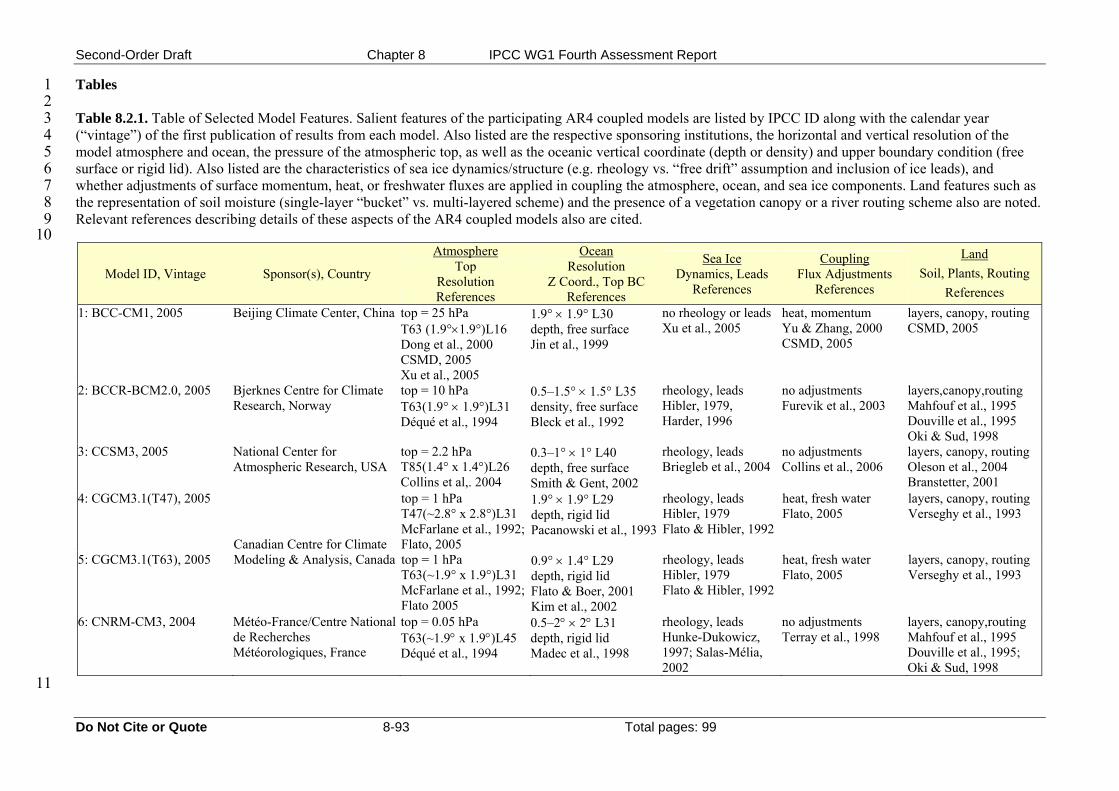
Second-Order Draft Chapter 8 IPCC WG1 Fourth Assessment Report
1 2 3 4 5 6 7 8 9
10
Tables Table 8.2.1. Table of Selected Model Features. Salient features of the participating AR4 coupled models are listed by IPCC ID along with the calendar year (“vintage”) of the first publication of results from each model. Also listed are the respective sponsoring institutions, the horizontal and vertical resolution of the model atmosphere and ocean, the pressure of the atmospheric top, as well as the oceanic vertical coordinate (depth or density) and upper boundary condition (free surface or rigid lid). Also listed are the characteristics of sea ice dynamics/structure (e.g. rheology vs. “free drift” assumption and inclusion of ice leads), and whether adjustments of surface momentum, heat, or freshwater fluxes are applied in coupling the atmosphere, ocean, and sea ice components. Land features such as the representation of soil moisture (single-layer “bucket” vs. multi-layered scheme) and the presence of a vegetation canopy or a river routing scheme also are noted. Relevant references describing details of these aspects of the AR4 coupled models also are cited.
Model ID, Vintage Sponsor(s), Country
Atmosphere Top
Resolution References
Ocean Resolution
Z Coord., Top BC References
Sea Ice Dynamics, Leads
References
Coupling Flux Adjustments
References
Land Soil, Plants, Routing
References 1: BCC-CM1, 2005 Beijing Climate Center, China top = 25 hPa
T63 (1.9°×1.9°)L16 Dong et al., 2000 CSMD, 2005 Xu et al., 2005
1.9° × 1.9° L30 depth, free surface Jin et al., 1999
no rheology or leads Xu et al., 2005
heat, momentum Yu & Zhang, 2000 CSMD, 2005
layers, canopy, routing CSMD, 2005
2: BCCR-BCM2.0, 2005 Bjerknes Centre for Climate Research, Norway
top = 10 hPa T63(1.9° × 1.9°)L31 Déqué et al., 1994
0.5–1.5° × 1.5° L35 density, free surface Bleck et al., 1992
rheology, leads Hibler, 1979, Harder, 1996
no adjustments Furevik et al., 2003
layers,canopy,routing Mahfouf et al., 1995 Douville et al., 1995 Oki & Sud, 1998
3: CCSM3, 2005 National Center for Atmospheric Research, USA
top = 2.2 hPa T85(1.4° x 1.4°)L26 Collins et al,. 2004
0.3–1° × 1° L40 depth, free surface Smith & Gent, 2002
rheology, leads Briegleb et al., 2004
no adjustments Collins et al., 2006
layers, canopy, routing Oleson et al., 2004 Branstetter, 2001
4: CGCM3.1(T47), 2005 top = 1 hPa T47(~2.8° x 2.8°)L31 McFarlane et al., 1992; Flato, 2005
1.9° × 1.9° L29 depth, rigid lid Pacanowski et al., 1993
rheology, leads Hibler, 1979 Flato & Hibler, 1992
heat, fresh water Flato, 2005
layers, canopy, routing Verseghy et al., 1993
5: CGCM3.1(T63), 2005
Canadian Centre for Climate Modeling & Analysis, Canada top = 1 hPa
T63(~1.9° x 1.9°)L31 McFarlane et al., 1992; Flato 2005
0.9° × 1.4° L29 depth, rigid lid Flato & Boer, 2001 Kim et al., 2002
rheology, leads Hibler, 1979 Flato & Hibler, 1992
heat, fresh water Flato, 2005
layers, canopy, routing Verseghy et al., 1993
6: CNRM-CM3, 2004 Météo-France/Centre National de Recherches Météorologiques, France
top = 0.05 hPa T63(~1.9° x 1.9°)L45 Déqué et al., 1994
0.5–2° × 2° L31 depth, rigid lid Madec et al., 1998
rheology, leads Hunke-Dukowicz, 1997; Salas-Mélia, 2002
no adjustments Terray et al., 1998
layers, canopy,routing Mahfouf et al., 1995 Douville et al., 1995; Oki & Sud, 1998
11
Do Not Cite or Quote 8-93 Total pages: 99
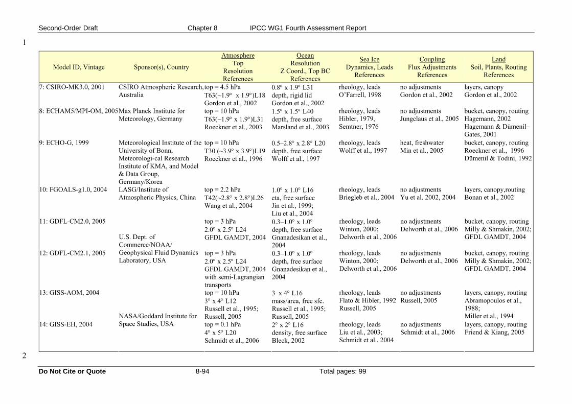
Second-Order Draft Chapter 8 IPCC WG1 Fourth Assessment Report
1
2
Model ID, Vintage Sponsor(s), Country
Atmosphere Top
Resolution References
Ocean Resolution
Z Coord., Top BC References
Sea Ice Dynamics, Leads
References
Coupling Flux Adjustments
References
Land Soil, Plants, Routing
References
7: CSIRO-MK3.0, 2001 CSIRO Atmospheric Research,Australia
top = 4.5 hPa T63(~1.9° x 1.9°)L18 Gordon et al., 2002
0.8° x 1.9° L31 depth, rigid lid Gordon et al., 2002
rheology, leads O’Farrell, 1998
no adjustments Gordon et al., 2002
layers, canopy Gordon et al., 2002
8: ECHAM5/MPI-OM, 2005Max Planck Institute for Meteorology, Germany
top = 10 hPa T63(~1.9° x 1.9°)L31 Roeckner et al., 2003
1.5° x 1.5° L40 depth, free surface Marsland et al., 2003
rheology, leads Hibler, 1979, Semtner, 1976
no adjustments Jungclaus et al., 2005
bucket, canopy, routing Hagemann, 2002 Hagemann & Dümenil–Gates, 2001
9: ECHO-G, 1999 Meteorological Institute of the University of Bonn, Meteorologi-cal Research Institute of KMA, and Model & Data Group, Germany/Korea
top = 10 hPa T30 (~3.9° x 3.9°)L19 Roeckner et al., 1996
0.5–2.8° x 2.8° L20 depth, free surface Wolff et al., 1997
rheology, leads Wolff et al., 1997
heat, freshwater Min et al., 2005
bucket, canopy, routing Roeckner et al., 1996 Dümenil & Todini, 1992
10: FGOALS-g1.0, 2004 LASG/Institute of Atmospheric Physics, China
top = 2.2 hPa T42(~2.8° x 2.8°)L26 Wang et al., 2004
1.0° x 1.0° L16 eta, free surface Jin et al., 1999; Liu et al., 2004
rheology, leads Briegleb et al., 2004
no adjustments Yu et al. 2002, 2004
layers, canopy,routing Bonan et al., 2002
11: GDFL-CM2.0, 2005 top = 3 hPa 2.0° x 2.5° L24 GFDL GAMDT, 2004
0.3–1.0° x 1.0° depth, free surface Gnanadesikan et al., 2004
rheology, leads Winton, 2000; Delworth et al., 2006
no adjustments Delworth et al., 2006
bucket, canopy, routing Milly & Shmakin, 2002; GFDL GAMDT, 2004
12: GDFL-CM2.1, 2005
U.S. Dept. of Commerce/NOAA/ Geophysical Fluid Dynamics Laboratory, USA
top = 3 hPa 2.0° x 2.5° L24 GFDL GAMDT, 2004 with semi-Lagrangian transports
0.3–1.0° x 1.0° depth, free surface Gnanadesikan et al., 2004
rheology, leads Winton, 2000; Delworth et al., 2006
no adjustments Delworth et al., 2006
bucket, canopy, routing Milly & Shmakin, 2002; GFDL GAMDT, 2004
13: GISS-AOM, 2004 top = 10 hPa 3° x 4° L12 Russell et al., 1995; Russell, 2005
3 x 4° L16 mass/area, free sfc. Russell et al., 1995; Russell, 2005
rheology, leads Flato & Hibler, 1992 Russell, 2005
no adjustments Russell, 2005
layers, canopy, routing Abramopoulos et al., 1988; Miller et al., 1994
14: GISS-EH, 2004
NASA/Goddard Institute for Space Studies, USA top = 0.1 hPa
4° x 5° L20 Schmidt et al., 2006
2° x 2° L16 density, free surface Bleck, 2002
rheology, leads Liu et al., 2003; Schmidt et al., 2004
no adjustments Schmidt et al., 2006
layers, canopy, routing Friend & Kiang, 2005
Do Not Cite or Quote 8-94 Total pages: 99
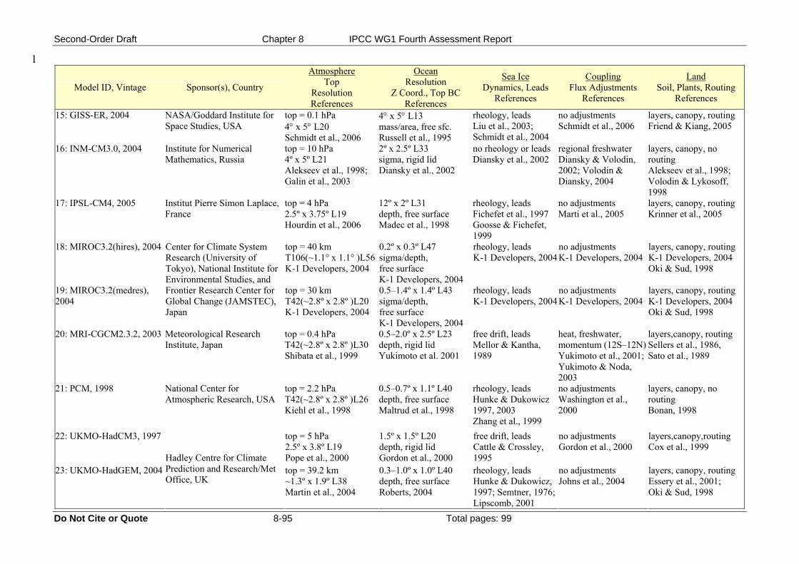
cond-Order Draft Chapter 8 IPCC WG1 Fourth Assessment Report
Do Not Cite or Quote 8-95 Total pages: 99
Model ID, Vintage Sponsor(s), Country
Atmosphere Top
Resolution References
Ocean Resolution
Z Coord., Top BC References
Sea Ice Dynamics, Leads
References
Coupling Flux Adjustments
References
Land Soil, Plants, Routing
References
15: GISS-ER, 2004 NASA/Goddard Institute for Space Studies, USA
top = 0.1 hPa 4° x 5° L20 Schmidt et al., 2006
4° x 5° L13 mass/area, free sfc. Russell et al., 1995
rheology, leads Liu et al., 2003; Schmidt et al., 2004
no adjustments Schmidt et al., 2006
layers, canopy, routing Friend & Kiang, 2005
16: INM-CM3.0, 2004 Institute for Numerical Mathematics, Russia
top = 10 hPa 4º x 5º L21 Alekseev et al., 1998; Galin et al., 2003
2º x 2.5º L33 sigma, rigid lid Diansky et al., 2002
no rheology or leads Diansky et al., 2002
regional freshwater Diansky & Volodin, 2002; Volodin & Diansky, 2004
layers, canopy, no routing Alekseev et al., 1998; Volodin & Lykosoff, 1998
17: IPSL-CM4, 2005 Institut Pierre Simon Laplace, France
top = 4 hPa 2.5º x 3.75º L19 Hourdin et al., 2006
12º x 2º L31 depth, free surface Madec et al., 1998
rheology, leads Fichefet et al., 1997 Goosse & Fichefet, 1999
no adjustments Marti et al., 2005
layers, canopy, routing Krinner et al., 2005
18: MIROC3.2(hires), 2004 top = 40 km T106(~1.1° x 1.1° )L56K-1 Developers, 2004
0.2º x 0.3º L47 sigma/depth, free surface K-1 Developers, 2004
rheology, leads K-1 Developers, 2004
no adjustments K-1 Developers, 2004
layers, canopy, routing K-1 Developers, 2004 Oki & Sud, 1998
19: MIROC3.2(medres), 2004
Center for Climate System Research (University of Tokyo), National Institute for Environmental Studies, and Frontier Research Center for Global Change (JAMSTEC), Japan
top = 30 km T42(~2.8º x 2.8º )L20 K-1 Developers, 2004
0.5–1.4º x 1.4º L43 sigma/depth, free surface K-1 Developers, 2004
rheology, leads K-1 Developers, 2004
no adjustments K-1 Developers, 2004
layers, canopy, routing K-1 Developers, 2004 Oki & Sud, 1998
20: MRI-CGCM2.3.2, 2003 Meteorological Research Institute, Japan
top = 0.4 hPa T42(~2.8º x 2.8º )L30 Shibata et al., 1999
0.5–2.0º x 2.5º L23 depth, rigid lid Yukimoto et al. 2001
free drift, leads Mellor & Kantha, 1989
heat, freshwater, momentum (12S–12N)Yukimoto et al., 2001;Yukimoto & Noda, 2003
layers,canopy, routing Sellers et al., 1986, Sato et al., 1989
21: PCM, 1998 National Center for Atmospheric Research, USA
top = 2.2 hPa T42(~2.8º x 2.8º )L26 Kiehl et al., 1998
0.5–0.7º x 1.1º L40 depth, free surface Maltrud et al., 1998
rheology, leads Hunke & Dukowicz 1997, 2003 Zhang et al., 1999
no adjustments Washington et al., 2000
layers, canopy, no routing Bonan, 1998
22: UKMO-HadCM3, 1997 top = 5 hPa 2.5º x 3.8º L19 Pope et al., 2000
1.5º x 1.5º L20 depth, rigid lid Gordon et al., 2000
free drift, leads Cattle & Crossley, 1995
no adjustments Gordon et al., 2000
layers,canopy,routing Cox et al., 1999
23: UKMO-HadGEM, 2004
Hadley Centre for Climate Prediction and Research/Met Office, UK
top = 39.2 km ~1.3º x 1.9º L38 Martin et al., 2004
0.3–1.0º x 1.0º L40 depth, free surface Roberts, 2004
rheology, leads Hunke & Dukowicz, 1997; Semtner, 1976;Lipscomb, 2001
no adjustments Johns et al., 2004
layers, canopy, routing Essery et al., 2001; Oki & Sud, 1998
Se
1
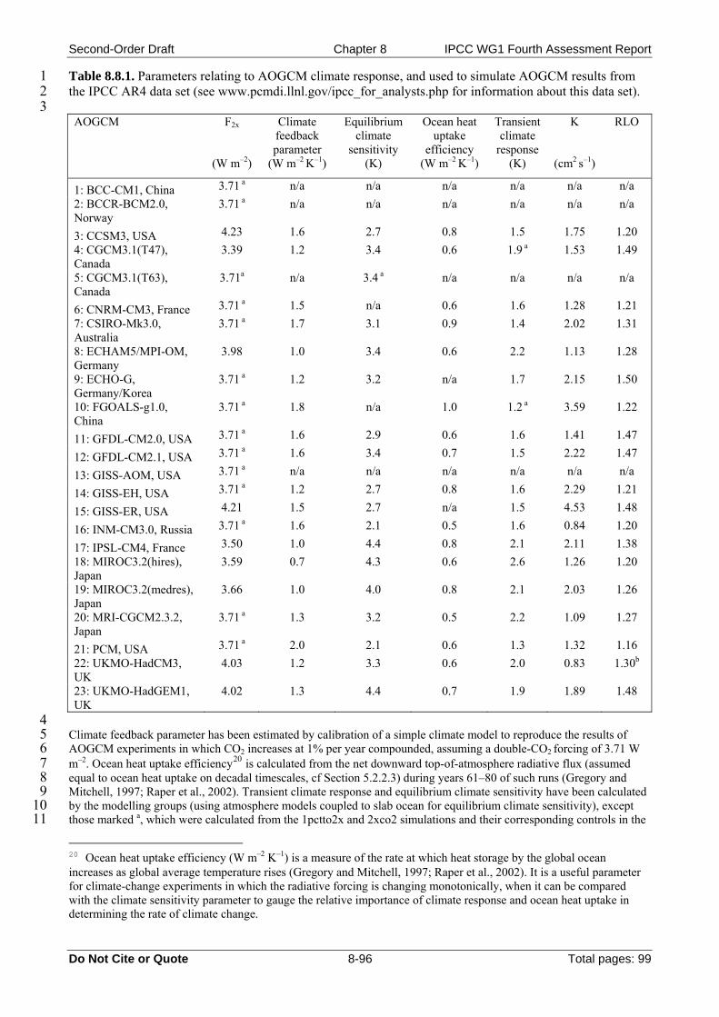
Second-Order Draft Chapter 8 IPCC WG1 Fourth Assessment Report
1 2 3
Table 8.8.1. Parameters relating to AOGCM climate response, and used to simulate AOGCM results from the IPCC AR4 data set (see www.pcmdi.llnl.gov/ipcc_for_analysts.php for information about this data set).
F2x Climate feedback parameter
Equilibrium climate
sensitivity
Ocean heat uptake
efficiency
Transient climate
response
K RLO AOGCM
(W m–2) (W m–2 K–1) (K) (W m–2 K–1) (K) (cm2 s–1)
1: BCC-CM1, China 3.71 a n/a n/a n/a n/a n/a n/a 2: BCCR-BCM2.0, Norway
3.71 a n/a n/a n/a n/a n/a n/a
3: CCSM3, USA 4.23 1.6 2.7 0.8 1.5 1.75 1.20 4: CGCM3.1(T47), Canada
3.39 1.2 3.4 0.6 1.9 a 1.53 1.49
5: CGCM3.1(T63), Canada
3.71a n/a 3.4 a n/a n/a n/a n/a
6: CNRM-CM3, France 3.71 a 1.5 n/a 0.6 1.6 1.28 1.21 7: CSIRO-Mk3.0, Australia
3.71 a 1.7 3.1 0.9 1.4 2.02 1.31
8: ECHAM5/MPI-OM, Germany
3.98 1.0 3.4 0.6 2.2 1.13 1.28
9: ECHO-G, Germany/Korea
3.71 a 1.2 3.2 n/a 1.7 2.15 1.50
10: FGOALS-g1.0, China
3.71 a 1.8 n/a 1.0 1.2 a 3.59 1.22
11: GFDL-CM2.0, USA 3.71 a 1.6 2.9 0.6 1.6 1.41 1.47
12: GFDL-CM2.1, USA 3.71 a 1.6 3.4 0.7 1.5 2.22 1.47
13: GISS-AOM, USA 3.71 a n/a n/a n/a n/a n/a n/a
14: GISS-EH, USA 3.71 a 1.2 2.7 0.8 1.6 2.29 1.21
15: GISS-ER, USA 4.21 1.5 2.7 n/a 1.5 4.53 1.48
16: INM-CM3.0, Russia 3.71 a 1.6 2.1 0.5 1.6 0.84 1.20
17: IPSL-CM4, France 3.50 1.0 4.4 0.8 2.1 2.11 1.38 18: MIROC3.2(hires), Japan
3.59 0.7 4.3 0.6 2.6 1.26 1.20
19: MIROC3.2(medres), Japan
3.66 1.0 4.0 0.8 2.1 2.03 1.26
20: MRI-CGCM2.3.2, Japan
3.71 a 1.3 3.2 0.5 2.2 1.09 1.27
21: PCM, USA 3.71 a 2.0 2.1 0.6 1.3 1.32 1.16 22: UKMO-HadCM3, UK
4.03 1.2 3.3 0.6 2.0 0.83 1.30b
23: UKMO-HadGEM1, UK
4.02 1.3 4.4 0.7 1.9 1.89 1.48
4 5 6 7 8 9
10 11
Climate feedback parameter has been estimated by calibration of a simple climate model to reproduce the results of AOGCM experiments in which CO2 increases at 1% per year compounded, assuming a double-CO2 forcing of 3.71 W m–2. Ocean heat uptake efficiency20 is calculated from the net downward top-of-atmosphere radiative flux (assumed equal to ocean heat uptake on decadal timescales, cf Section 5.2.2.3) during years 61–80 of such runs (Gregory and Mitchell, 1997; Raper et al., 2002). Transient climate response and equilibrium climate sensitivity have been calculated by the modelling groups (using atmosphere models coupled to slab ocean for equilibrium climate sensitivity), except those marked a, which were calculated from the 1pctto2x and 2xco2 simulations and their corresponding controls in the
20 Ocean heat uptake efficiency (W m–2 K–1) is a measure of the rate at which heat storage by the global ocean increases as global average temperature rises (Gregory and Mitchell, 1997; Raper et al., 2002). It is a useful parameter for climate-change experiments in which the radiative forcing is changing monotonically, when it can be compared with the climate sensitivity parameter to gauge the relative importance of climate response and ocean heat uptake in determining the rate of climate change. Do Not Cite or Quote 8-96 Total pages: 99

Second-Order Draft Chapter 8 IPCC WG1 Fourth Assessment Report
Do Not Cite or Quote 8-97 Total pages: 99
AR4 database. The evaluation of all of these quantities has some systematic uncertainty reflecting precise choice of method; climate feedback parameter and ocean heat uptake efficiency have a standard error of estimate of 0.1 W m
1 2 3 4 5 6 7 8 9
10
–2 K–
1, equilibrium climate sensitivity and transient climate response of 0.1 K. Notes: F2x: radiative forcing for doubled CO2 concentration K: ocean effective vertical diffusivity RLO: ratio of the equilibrium temperature changes over land versus ocean (a) Here the best estimate from Myhre et al. (1998) is used (b) Due to missing land ocean temperature data, the RLO parameter has been assumed as 1.3
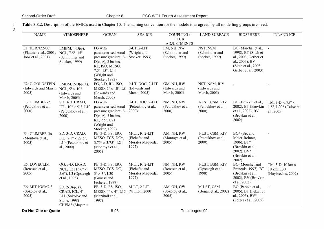
Second-Order Draft Chapter 8 IPCC WG1 Fourth Assessment Report
1 2
Table 8.8.2. Description of the EMICs used in Chapter 10. The naming convention for the models is as agreed by all modelling groups involved.
NAME ATMOSPHERE OCEAN SEA ICE COUPLING / FLUX
ADJUSTMENTS
LAND SURFACE BIOSPHERE INLAND ICE
E1 :BERN2.5CC (Plattner et al., 2001; Joos et al., 2001)
EMBM, 1-D(ϕ), NCL, 7.5°–15° (Schmittner and Stocker, 1999)
FG with parameterised zonal pressure gradient, 2-D(ϕ, z), 3 basins, RL, ISO, MESO, 7.5°–15°, L14 (Wright and Stocker, 1992)
0-LT, 2-LIT (Wright and Stocker, 1993)
PM, NH, NW (Schmittner and Stocker, 1999)
NST, NSM (Schmittner and Stocker, 1999)
BO (Marchal et al., 1998), BT (Sitch et al., 2003; Gerber et al., 2003), BV (Sitch et al., 2003; Gerber et al., 2003)
-
E2: C-GOLDSTEIN (Edwards and Marsh, 2005)
EMBM, 2-D(ϕ, λ), NCL, 5° × 10° (Edwards and Marsh, 2005)
FG, 3-D, RL, ISO, MESO, 5° × 10°, L8 (Edwards and Marsh, 2005)
0-LT, DOC, 2-LIT (Edwards and Marsh, 2005)
GM, NH, RW (Edwards and Marsh, 2005)
NST, NSM, RIV (Edwards and Marsh, 2005)
- -
E3: CLIMBER-2 (Petoukhov et al., 2000)
SD, 3-D, CRAD, ICL, 10° × 51°, L10 (Petoukhov et al., 2000)
FG with parameterised zonal pressure gradient, 2-D(ϕ, z), 3 basins, RL, 2.5°, L21 (Wright and Stocker, 1992)
0-LT, DOC, 2-LIT (Petoukhov et al., 2000)
NM, NH, NW (Petoukhov et al., 2000)
1-LST, CSM, RIV (Petoukhov et al., 2000)
BO (Brovkin et al., 2002), BT (Brovkin et al., 2002), BV (Brovkin et al., 2002)
TM, 3-D, 0.75° × 1.5°, L20* (Calov et al., 2005)
E4: CLIMBER-3α (Montoya et al., 2005)
SD, 3-D, CRAD, ICL, 7.5° × 22.5°, L10 (Petoukhov et al., 2000)
PE, 3-D, FS, ISO, MESO, TCS, DC*, 3.75° × 3.75°, L24 (Montoya et al., 2005)
M-LT, R, 2-LIT (Fichefet and Morales Maqueda, 1997)
AM, NH, RW (Montoya et al., 2005)
1-LST, CSM, RIV (Petoukhov et al., 2000)
BO* (Six and Maier-Reimer, 1996), BT* (Brovkin et al., 2002), BV* (Brovkin et al., 2002)
-
E5: LOVECLIM (Renssen et al., 2005)
QG, 3-D, LRAD, NCL, T21 (5.6° × 5.6°), L3 (Opsteegh et al., 1998)
PE, 3-D, FS, ISO, MESO, TCS, DC, 3° × 3°, L30 (Goosse and Fichefet, 1999)
M-LT, R, 2-LIT (Fichefet and Morales Maqueda, 1997)
NM, NH, RW (Renssen et al., 2005)
1-LST, BSM, RIV (Opsteegh et al., 1998)
BO (Mouchet and François, 1997), BT (Brovkin et al., 2002), BV (Brovkin et a., 2002)
TM, 3-D, 10 km × 10 km, L30 (Huybrechts, 2002)
E6: MIT-IGSM2.3 (Sokolov et al., 2005)
SD, 2-D(ϕ, z), CRAD, ICL, 4°, L11 (Sokolov and Stone, 1998) CHEM* (Mayer et
PE, 3-D, FS, ISO, MESO, 4° × 4°, L15 (Marshall et al., 1997)
M-LT, 2-LIT (Winton, 2000)
AM, GH, GW (Sokolov et al., 2005)
M-LST, CSM (Bonan et al., 2002)
BO (Parekh et al., 2005), BT (Felzer et al., 2005), BV* (Felzer et al., 2005)
-
Do Not Cite or Quote 8-98 Total pages: 99
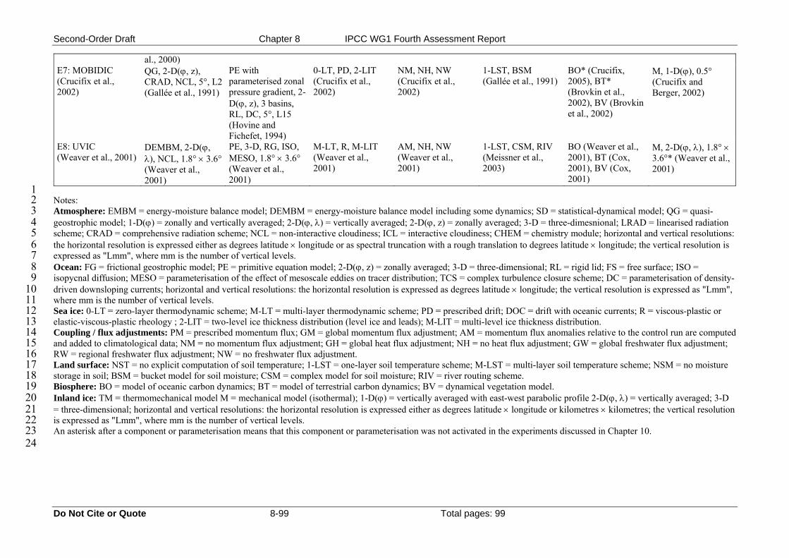
Second-Order Draft Chapter 8 IPCC WG1 Fourth Assessment Report
al., 2000) E7: MOBIDIC (Crucifix et al., 2002)
QG, 2-D(ϕ, z), CRAD, NCL, 5°, L2 (Gallée et al., 1991)
PE with parameterised zonal pressure gradient, 2-D(ϕ, z), 3 basins, RL, DC, 5°, L15 (Hovine and Fichefet, 1994)
0-LT, PD, 2-LIT (Crucifix et al., 2002)
NM, NH, NW (Crucifix et al., 2002)
1-LST, BSM (Gallée et al., 1991)
BO* (Crucifix, 2005), BT* (Brovkin et al., 2002), BV (Brovkin et al., 2002)
M, 1-D(ϕ), 0.5° (Crucifix and Berger, 2002)
E8: UVIC (Weaver et al., 2001)
DEMBM, 2-D(ϕ, λ), NCL, 1.8° × 3.6° (Weaver et al., 2001)
PE, 3-D, RG, ISO, MESO, 1.8° × 3.6° (Weaver et al., 2001)
M-LT, R, M-LIT (Weaver et al., 2001)
AM, NH, NW (Weaver et al., 2001)
1-LST, CSM, RIV (Meissner et al., 2003)
BO (Weaver et al., 2001), BT (Cox, 2001), BV (Cox, 2001)
M, 2-D(ϕ, λ), 1.8° × 3.6°* (Weaver et al., 2001)
1 2 3 4 5 6 7 8 9
10 11 12 13 14 15 16 17 18 19 20 21 22 23 24
Notes: Atmosphere: EMBM = energy-moisture balance model; DEMBM = energy-moisture balance model including some dynamics; SD = statistical-dynamical model; QG = quasi-geostrophic model; 1-D(ϕ) = zonally and vertically averaged; 2-D(ϕ, λ) = vertically averaged; 2-D(ϕ, z) = zonally averaged; 3-D = three-dimesnional; LRAD = linearised radiation scheme; CRAD = comprehensive radiation scheme; NCL = non-interactive cloudiness; ICL = interactive cloudiness; CHEM = chemistry module; horizontal and vertical resolutions: the horizontal resolution is expressed either as degrees latitude × longitude or as spectral truncation with a rough translation to degrees latitude × longitude; the vertical resolution is expressed as "Lmm", where mm is the number of vertical levels. Ocean: FG = frictional geostrophic model; PE = primitive equation model; 2-D(ϕ, z) = zonally averaged; 3-D = three-dimensional; RL = rigid lid; FS = free surface; ISO = isopycnal diffusion; MESO = parameterisation of the effect of mesoscale eddies on tracer distribution; TCS = complex turbulence closure scheme; DC = parameterisation of density-driven downsloping currents; horizontal and vertical resolutions: the horizontal resolution is expressed as degrees latitude × longitude; the vertical resolution is expressed as "Lmm", where mm is the number of vertical levels. Sea ice: 0-LT = zero-layer thermodynamic scheme; M-LT = multi-layer thermodynamic scheme; PD = prescribed drift; DOC = drift with oceanic currents; R = viscous-plastic or elastic-viscous-plastic rheology ; 2-LIT = two-level ice thickness distribution (level ice and leads); M-LIT = multi-level ice thickness distribution. Coupling / flux adjustments: PM = prescribed momentum flux; GM = global momentum flux adjustment; AM = momentum flux anomalies relative to the control run are computed and added to climatological data; NM = no momentum flux adjustment; GH = global heat flux adjustment; NH = no heat flux adjustment; GW = global freshwater flux adjustment; RW = regional freshwater flux adjustment; NW = no freshwater flux adjustment. Land surface: NST = no explicit computation of soil temperature; 1-LST = one-layer soil temperature scheme; M-LST = multi-layer soil temperature scheme; NSM = no moisture storage in soil; BSM = bucket model for soil moisture; CSM = complex model for soil moisture; RIV = river routing scheme. Biosphere: BO = model of oceanic carbon dynamics; BT = model of terrestrial carbon dynamics; BV = dynamical vegetation model. Inland ice: TM = thermomechanical model M = mechanical model (isothermal); 1-D(ϕ) = vertically averaged with east-west parabolic profile 2-D(ϕ, λ) = vertically averaged; 3-D = three-dimensional; horizontal and vertical resolutions: the horizontal resolution is expressed either as degrees latitude × longitude or kilometres × kilometres; the vertical resolution is expressed as "Lmm", where mm is the number of vertical levels. An asterisk after a component or parameterisation means that this component or parameterisation was not activated in the experiments discussed in Chapter 10.
Do Not Cite or Quote 8-99 Total pages: 99