Embed Size (px)
Citation preview
1
Characterizing the Impact of Horizontal HeatTransfer on the Linear Relation of Heat Flow
and Heat Production
Ronald G. ResminiDepartment of Geography and GeoInformation Science
College of ScienceGeorge Mason University
4400 University Drive, MSN 6C3Fairfax, VA 22030-4444
v: 703-470-3022 · e: [email protected]
2
Horizontal heat transfer impacts the linear relation between heat flowand heat production
Derived reduced heat flow and heat production depth values do not matchactual values
Reduced heat flows are higher; depth values are lower
A method for characterizing the impact of horizontal heat transferis presented here
It is applicable to the uniform heat production model for two-dimensionalheat transfer
The method suggests an approach for correcting the effects of horizontalheat transfer
Introduction

3
Procedure (1 of 6)
Construct a two-dimensional heat transfer model implementing theuniform heat production distribution
The depth of the uniform heat production domains is constant across the two-dimensional heat transfer model space
E.g., a model with five heat production domains is shown:

4
Procedure (2 of 6) Obtain the steady-state temperature field for the model
This is done analytically and numerically (see next slide)
For every model, basal heat flow, Qf, is always 25.0 mW/m2
Thermal conductivity, kT, is always 2.85 W/m.°C
Calculate the linear heat flow/heat production (intercept and slope) parameters
Note that they will not match the parameters of the forward model
Repeat the previous steps...but decrease the depth to the base of the heatproduction domains...keeping the same heat production values and theirspatial distribution
I.e., construct another two-dimensional heat transfer model implementing theuniform heat production distribution but with a depth to the base of theheat production domains 1 km less than the previous model
As before, the depth of the uniform heat production domains is still constantacross the two-dimensional heat transfer model space

5
A1
mW/m3
A2
mW/m3
A3
mW/m3
A4
mW/m3
A5
mW/m3
0.00mW/m3
125 km
35 km0x
T
0x
T
T
f
k
Q
y
T
0y
T
x
T2
2
2
2
0j T
j
2
2
2
2
L
xjcos
k
c
y
T
x
Tand
x = 0 x = Ly = H
y = 0T = 0
The Problem Space
Other models in this study are 250 kilometers in width (x-direction).
y = b
6
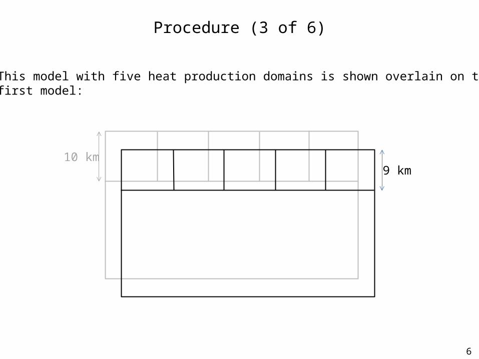
Procedure (3 of 6)
• This model with five heat production domains is shown overlain on the first model:
9 km10 km
7
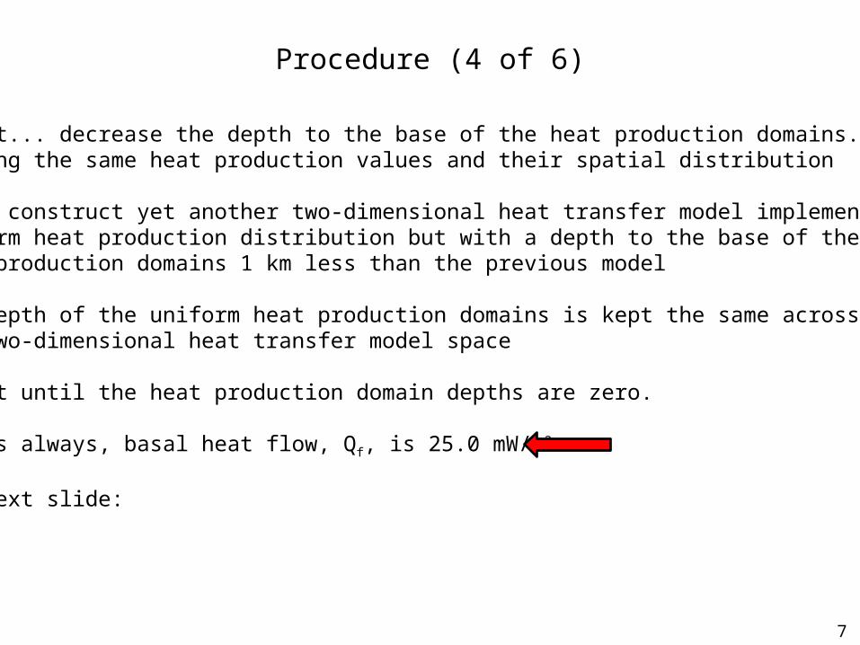
Procedure (4 of 6)
Repeat... decrease the depth to the base of the heat production domains...keeping the same heat production values and their spatial distribution
I.e., construct yet another two-dimensional heat transfer model implementing theuniform heat production distribution but with a depth to the base of theheat production domains 1 km less than the previous model
The depth of the uniform heat production domains is kept the same acrossthe two-dimensional heat transfer model space
Repeat until the heat production domain depths are zero.
And as always, basal heat flow, Qf, is 25.0 mW/m2
See next slide:
8
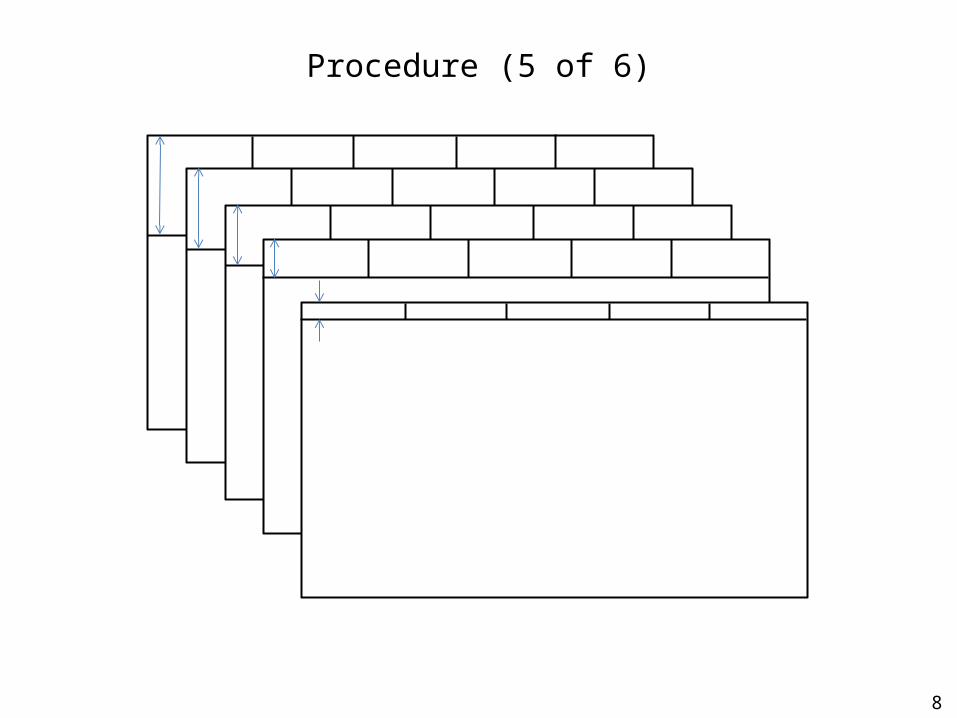
Procedure (5 of 6)

9
Procedure (6 of 6)
Thirteen (13) such two-dimensional models were calculated and fromwhich 13 pairs of heat flow/heat production linear parameters were derived:
Depth to base of heat production region: 10, 9, 8, 7, 6, 5, 4, 3,2, 1, 0.5, 0.1, 0 km
A plot of intercept values (reduced heat flow), Y-axis, vs. values oftrue depth to the base of the heat production domains minus the slope(true depth – slope), X-axis, is constructed
The plot has 13 points
The plot has two linear portions
A line is fit to the predominant linear portion (see next slides)
The slope has the units of heat production, mW/m3
The intercept has the units of heat flow, mW/m2
10
T
sd kd
TTQ
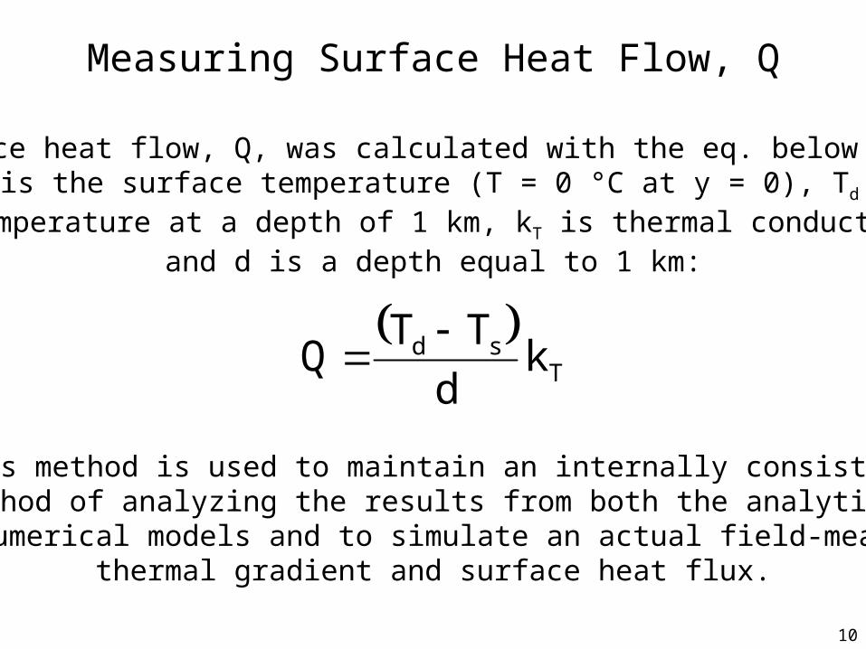
Surface heat flow, Q, was calculated with the eq. below whereTs is the surface temperature (T = 0 °C at y = 0), Td is
the temperature at a depth of 1 km, kT is thermal conductivity,and d is a depth equal to 1 km:
This method is used to maintain an internally consistentmethod of analyzing the results from both the analytical
and numerical models and to simulate an actual field-measuredthermal gradient and surface heat flux.
Measuring Surface Heat Flow, Q

11
Tools
• Pencil-’n-paper for analytical calculations
Subsequently implemented in C and Pascal(!) www.freepascal.org
• The FlexPDE© finite element software system
www.pdesolutions.com
• MS Excel©

12
0.00
1.00
2.00
3.00
4.00
5.00
6.00
7.00
0 25 50 75 100 125
Model 1a (Mod1a)
3.75 mW/m3
1.00 mW/m3
4.35 mW/m3
2.25 mW/m3
6.50 mW/m3
3.75 mW
/m3
1.00 mW
/m3
4.35 mW
/m3
2.25 mW
/m3
6.50 mW
/m3
Distance , x direction, kilometers
Hea
t Pro
ducti
on, A
, mW
/m3
Results
• Model 1a (Mod1a) is comprised of five heat flow domains andis shown below:

13
3.75mW/m3
1.00mW/m3
4.35mW/m3
2.25mW/m3
6.50mW/m3
0.00mW/m3
I.e., Model 1a is:
125 km
35 km

14
Temperature at a depth of 1 km – Model 1a
Analytical and numerical solutions are identical.
0
5
10
15
20
25
30
35
0 25 50 75 100 125
Numerical
Analytical
Distance in the x-Direction (Km)
Tem
pera
ture
(C)
Analytical and Numerical Solutions

15
Temperature at a depth of 35 km – Model 1a
Analytical and numerical solutions are identical.
Distance in the x-Direction (Km)
Tem
pera
ture
(C)
Analytical and Numerical Solutions

16
Mod1a Heat Flow Vectors

17
Model 1a (Mod 1a)
The linear relation between surface heat flow (Q) and the heat production (A)of rocks exposed at the surface for Model 1a:
True depth: 10 km; true basal heat flow, Q, 25.0 mW/m2
Note that retrieved depth (slope) is <10 km (7.04 km) and theretrieved reduced heat flow (intercept) is >25.0 mW/m2 (33.85 mW/m2)
y = 7.0358x + 33.845R² = 0.9749
20
30
40
50
60
70
80
90
0.00 1.00 2.00 3.00 4.00 5.00 6.00 7.00
Radiogenic Heat Production, A, mW/m3
Surf
ace
heat
Flo
w, Q
, mW
/m2

18
Model 1a (Mod 1a)
• There are 12 more such plots for Model 1a...
• There are 13 pairs of Q-A depth and reduced heat flow values
• They are shown in the table below along with the calculation of(true depth, b – slope):
True Depth Slope (Depth) True-Slope Intercept(km) (km) (km) (mW/m2)
10.0 7.04 2.96 33.859.0 6.47 2.53 32.288.0 5.87 2.13 30.847.0 5.24 1.76 29.546.0 4.56 1.44 28.385.0 3.84 1.16 27.374.0 3.07 0.93 26.533.0 2.26 0.74 25.872.0 1.39 0.61 25.391.0 0.47 0.53 25.100.5 0.12 0.38 25.020.1 0.00 0.10 25.000.0 0.00 0.00 25.00
Intercept values converge to 25.0 mW
/m2
Note
X-axis Y-axis...on plot on
next slide

19
Model 1a (Mod 1a)
The slope of the linear portion is 3.59 mW/m3 – remarkably close to 3.57 mW/m3
The intercept is also close to the true basal heat flux of 25.0 mW/m2
y = 3.5896x + 23.206R² = 1
20.00
22.00
24.00
26.00
28.00
30.00
32.00
34.00
36.00
0.0 0.5 1.0 1.5 2.0 2.5 3.0 3.5
Inte
rcep
t, Re
duce
d H
eat F
low
, Q, m
W/m
2
True Depth – Slope (km)
Ten (10) points form a sloping linear segment.
The linear regression is basedon the 10 points

20
What is 3.57 mW/m3?
HPE = Heat Producing Element
333333
mW57.3km25km25km25km25km25
mW50.6xkm25mW25.2xkm25mW35.4xkm25mW00.1xkm25mW75.3xkm25
It’s a distance-weighted average of theheat production values in the problem space:
One only needs to know the HPE values along the surface of the problem space.(Readily obtainable from field and laboratory analyses.)
n
1ii
n
1iii
width
HPExwidth.Avg

21
This Intercept vs. Depth – Slope relationship
is general; i.e., as will be shown next, it
obtains when applied to several different models
each with an average heat production value of
3.57 mW/m3. Models with other average
heat production values are shown, too.

22
More Analyses• Eleven (11) sets of 13 two-dimensional model calculations were
completed in the present study
• The problem domains are 125 km and 250 km in width
• All problem domains are 35 km in depth (y direction)
• The model configurations are given in the next several slides
• Many of the models were configured so that the average heatproduction value is 3.57 mW/m3
• One model has unphysical heat production values to purposelyyield an average of 0.0 mW/m3
• The heat production domain widths are varied
• Qf, applied basal heat flow, is always 25.0 mW/m2
• The linear heat flow vs. (true depth – slope) relation is obtained

23
n
1ii
n
1iii
width
HPExwidth.Avg
HPE = Heat Producing Element
333333
mW57.3km25km25km25km25km25
mW50.6xkm25mW25.2xkm25mW35.4xkm25mW00.1xkm25mW75.3xkm25
Distance Width Mod1a Mod1 Mod2 Mod3 Mod4 Mod5 Mod6 Mod7 Mod8 Mod9 Mod10(km) (km) (W/m3) (W/m3) (W/m3) (W/m3) (W/m3) (W/m3) (W/m3) (W/m3) (W/m3) (W/m3) (W/m3)
25 25 3.75 3.75 3.75 3.50 3.50 6.50 0.70 0.70 0.70 2.15 2.15
50 25 1.00 3.75 1.00 2.75 2.75 1.00 1.50 0.70 3.85 6.25 2.15
75 25 4.35 1.00 4.35 6.50 0.00 1.00 2.90 0.70 7.50 1.60 2.15
100 25 2.25 1.00 2.25 1.25 -2.75 1.00 3.85 3.85 0.70 2.15 2.15
125 25 6.50 4.35 6.50 4.65 -3.50 1.00 2.00 3.85 3.20 6.25 6.25
150 25 4.35 3.75 3.25 5.45 3.85 3.85 0.50 6.25
175 25 2.25 1.00 3.25 3.65 3.85 0.70 2.15 6.25
200 25 2.25 4.35 2.75 7.75 7.75 3.85 6.25 6.25
225 25 6.50 2.25 2.75 5.00 7.75 7.50 2.15 1.60
250 25 6.50 6.50 2.75 2.90 3.20 3.85 6.25 0.50
Avg.: 3.57 3.57 3.57 3.73 0.00 2.53 3.57 3.62 3.57 3.57 3.57

24
0.00
1.00
2.00
3.00
4.00
5.00
6.00
7.00
0 25 50 75 100 125 150 175 200 225 250
Model 1 (Mod1)
3.75 mW
/m3
1.00 mW
/m3
4.35 mW
/m3
2.25 mW
/m3
6.50 mW
/m3
3.75 mW/m3
1.00 mW/m3
4.35 mW/m3
2.25 mW/m3
6.50 mW/m3
Distance , x direction, kilometers
Hea
t Pro
ducti
on, A
, mW
/m3
...similar to Mod1a exceptthe problem space is longerin the horizontal direction

25
Model 1 (Mod1)
y = 8.3421x + 29.134R² = 0.9942
0.0
10.0
20.0
30.0
40.0
50.0
60.0
70.0
80.0
90.0
0.00 1.00 2.00 3.00 4.00 5.00 6.00 7.00
Radiogenic Heat Production, A, mW/m3
Surf
ace
heat
Flo
w, Q
, mW
/m2
The linear relation between surface heat flow (Q) and the heat production (A)of rocks exposed at the surface for Model 1:
True depth: 10 km; true basal heat flow, Qf, 25.0 mW/m2

26
Model 1 (Mod1)
Inte
rcep
t, m
W/m
2
Depth – Slope, km
y = 3.57x + 23.215R² = 1
20.0
22.0
24.0
26.0
28.0
30.0
0.00 0.25 0.50 0.75 1.00 1.25 1.50 1.75 2.00
27
0.00
1.00
2.00
3.00
4.00
5.00
6.00
7.00
0 25 50 75 100 125 150 175 200 225 250
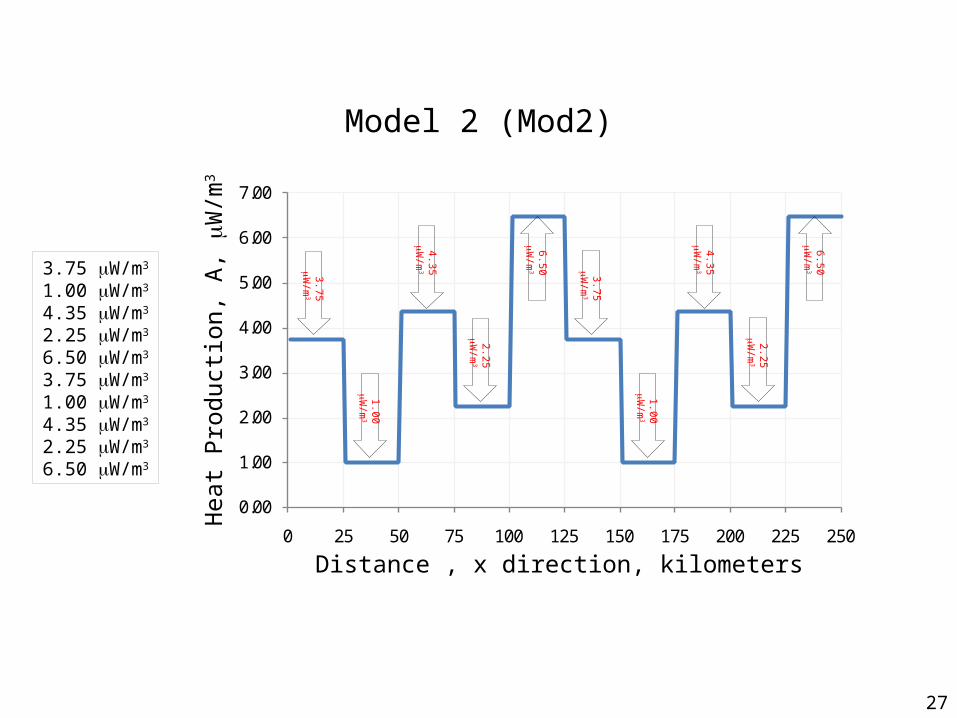
Model 2 (Mod2)
Distance , x direction, kilometers
Hea
t Pro
ducti
on, A
, mW
/m3
3.75 mW/m3
1.00 mW/m3
4.35 mW/m3
2.25 mW/m3
6.50 mW/m3
3.75 mW/m3
1.00 mW/m3
4.35 mW/m3
2.25 mW/m3
6.50 mW/m3
3.75 m
W/m
3
1.00 m
W/m
3
4.35 m
W/m
3
2.25 m
W/m
3
6.50 m
W/m
3 3.75 m
W/m
3
1.00 m
W/m
3
4.35 m
W/m
3
2.25 m
W/m
3
6.50 m
W/m
3

28
Model 2 (Mod2)
y = 6.8196x + 34.593R² = 0.9807
0.0
10.0
20.0
30.0
40.0
50.0
60.0
70.0
80.0
90.0
0.00 1.00 2.00 3.00 4.00 5.00 6.00 7.00
Radiogenic Heat Production, A, mW/m3
Surf
ace
heat
Flo
w, Q
, mW
/m2
The linear relation between surface heat flow (Q) and the heat production (A)of rocks exposed at the surface for Model 2:
True depth: 10 km; true basal heat flow, Qf, 25.0 mW/m2

29
Model 2 (Mod2)
Depth – Slope, km
Inte
rcep
t, m
W/m
2 y = 3.5789x + 23.211R² = 1
20.0
22.0
24.0
26.0
28.0
30.0
32.0
34.0
36.0
0.00 0.50 1.00 1.50 2.00 2.50 3.00 3.50
30
0.00
1.00
2.00
3.00
4.00
5.00
6.00
7.00
0 25 50 75 100 125
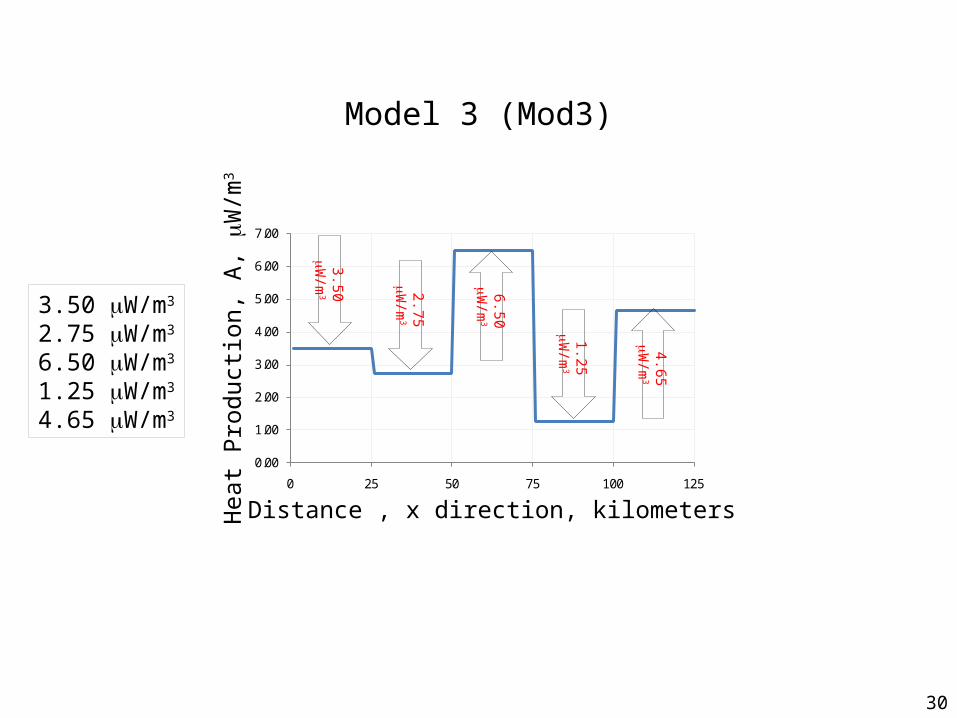
Model 3 (Mod3)
Distance , x direction, kilometers
Hea
t Pro
ducti
on, A
, mW
/m3
3.50 mW
/m3
2.75 mW
/m3
6.50 mW
/m3
1.25 mW
/m3
4.65 mW
/m3
3.50 mW/m3
2.75 mW/m3
6.50 mW/m3
1.25 mW/m3
4.65 mW/m3

31
Depth – Slope, km
Inte
rcep
t, m
W/m
2
y = 3.7344x + 23.134R² = 1
20.0
22.0
24.0
26.0
28.0
30.0
32.0
34.0
36.0
38.0
40.0
0.00 0.50 1.00 1.50 2.00 2.50 3.00 3.50 4.00
Model 3 (Mod3)
32
-4.00
-3.00
-2.00
-1.00
0.00
1.00
2.00
3.00
4.00
0 25 50 75 100 125
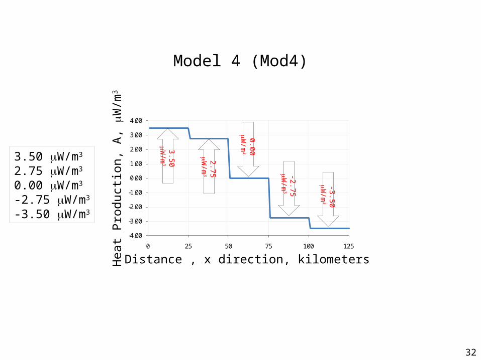
Model 4 (Mod4)
Distance , x direction, kilometers
Hea
t Pro
ducti
on, A
, mW
/m3
3.50 mW/m3
2.75 mW/m3
0.00 mW/m3
-2.75 mW/m3
-3.50 mW/m3
3.50 mW
/m3
2.75 mW
/m3
0.00 mW
/m3
-2.75 m
W/m
3
-3.50 m
W/m
3

33
Model 4 (Mod4)
Depth – Slope, km
Inte
rcep
t, m
W/m
2 y = -0.1122x + 25.037R² = 0.8657
20.0
22.5
25.0
27.5
30.0
0.00 0.20 0.40 0.60 0.80 1.00 1.20 1.40 1.60
34
0.00
1.00
2.00
3.00
4.00
5.00
6.00
7.00
0 25 50 75 100 125 150 175 200 225 250
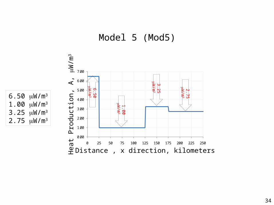
Model 5 (Mod5)
Distance , x direction, kilometers
Hea
t Pro
ducti
on, A
, mW
/m3
6.50 mW/m3
1.00 mW/m3
3.25 mW/m3
2.75 mW/m3
6.50 mW
/m3
1.00 mW
/m3
3.25 mW
/m3
2.75 mW
/m3

35
Model 5 (Mod5)
Depth – Slope, km
Inte
rcep
t, m
W/m
2 y = 2.5101x + 23.744R² = 1
20.0
22.0
24.0
26.0
28.0
30.0
0.00 0.50 1.00 1.50 2.00 2.50

36
0.00
1.00
2.00
3.00
4.00
5.00
6.00
7.00
8.00
9.00
0 25 50 75 100 125 150 175 200 225 250
Model 6 (Mod6)
Distance , x direction, kilometers
Hea
t Pro
ducti
on, A
, mW
/m3
0.70 mW/m3
1.50 mW/m3
2.90 mW/m3
3.85 mW/m3
2.00 mW/m3
5.45 mW/m3
3.65 mW/m3
7.75 mW/m3
5.00 mW/m3
2.90 mW/m3
0.70 m
W/m
3
1.50 m
W/m
3
2.90 m
W/m
3
3.85 m
W/m
3
2.00 m
W/m
3
5.45 m
W/m
3
3.65 m
W/m
3
7.75 m
W/m
3
5.00 m
W/m
3
2.90 m
W/m
3

37
y = 7.998x + 30.387R² = 0.974
0.0
10.0
20.0
30.0
40.0
50.0
60.0
70.0
80.0
90.0
100.0
0.00 2.00 4.00 6.00 8.00 10.00
Model 6 (Mod6)
Radiogenic Heat Production, A, mW/m3
Surf
ace
heat
Flo
w, Q
, mW
/m2
The linear relation between surface heat flow (Q) and the heat production (A)of rocks exposed at the surface for Model 6:
True depth: 10 km; true basal heat flow, Qf, 25.0 mW/m2

38
Model 6 (Mod6)
Depth – Slope, km
Inte
rcep
t, m
W/m
2 y = 3.5864x + 23.207R² = 1
20.0
22.0
24.0
26.0
28.0
30.0
32.0
0.00 0.50 1.00 1.50 2.00 2.50

39
0.00
1.00
2.00
3.00
4.00
5.00
6.00
7.00
8.00
9.00
0 25 50 75 100 125 150 175 200 225 250
Model 7 (Mod7)
Distance , x direction, kilometers
Hea
t Pro
ducti
on, A
, mW
/m3
0.70 mW/m3
3.85 mW/m3
7.75 mW/m3
3.20 mW/m3
0.70 mW
/m3
3.85 mW
/m3
7.75 mW
/m3
3.20 mW
/m3

40
Model 7 (Mod7)
The linear relation between surface heat flow (Q) and the heat production (A)of rocks exposed at the surface for Model 7:
True depth: 10 km; true basal heat flow, Qf, 25.0 mW/m2
Radiogenic Heat Production, A, mW/m3
Surf
ace
heat
Flo
w, Q
, mW
/m2
y = 8.4601x + 28.797R² = 0.9839
0.0
10.0
20.0
30.0
40.0
50.0
60.0
70.0
80.0
90.0
100.0
0.00 2.00 4.00 6.00 8.00 10.00

41
Model 7 (Mod7)
Depth – Slope, km
Inte
rcep
t, m
W/m
2
y = 3.6518x + 23.174
R² = 1
20.0
21.0
22.0
23.0
24.0
25.0
26.0
27.0
28.0
29.0
30.0
0.00 0.50 1.00 1.50 2.00

42
0.00
1.00
2.00
3.00
4.00
5.00
6.00
7.00
8.00
0 25 50 75 100 125 150 175 200 225 250
Model 8 (Mod8)
Distance , x direction, kilometers
Hea
t Pro
ducti
on, A
, mW
/m3
0.70 mW/m3
3.85 mW/m3
7.50 mW/m3
0.70 mW/m3
3.20 mW/m3
3.85 mW/m3
0.70 mW/m3
3.85 mW/m3
7.50 mW/m3
3.85 mW/m3
0.70 m
W/m
3
3.85 m
W/m
3
7.50 m
W/m
3
0.70 m
W/m
3
3.20 m
W/m
3
3.85 m
W/m
3
0.70 m
W/m
3
3.85 m
W/m
3
7.50 m
W/m
3
3.85 m
W/m
3

43
y = 7.0108x + 33.916R² = 0.985
0.0
10.0
20.0
30.0
40.0
50.0
60.0
70.0
80.0
90.0
100.0
0.00 1.00 2.00 3.00 4.00 5.00 6.00 7.00 8.00
Model 8 (Mod8)
Radiogenic Heat Production, A, mW/m3
Surf
ace
heat
Flo
w, Q
, mW
/m2
The linear relation between surface heat flow (Q) and the heat production (A)of rocks exposed at the surface for Model 8:
True depth: 10 km; true basal heat flow, Qf, 25.0 mW/m2

44
Model 8 (Mod8)
y = 3.582x + 23.209R² = 1
20.0
22.0
24.0
26.0
28.0
30.0
32.0
34.0
36.0
0.00 0.50 1.00 1.50 2.00 2.50 3.00 3.50
Depth – Slope, km
Inte
rcep
t, m
W/m
2

45
Model 9 (Mod9)
0.00
1.00
2.00
3.00
4.00
5.00
6.00
7.00
0 25 50 75 100 125 150 175 200 225 250
Distance , x direction, kilometers
Hea
t Pro
ducti
on, A
, mW
/m3
2.15 m
W/m
3
6.25 m
W/m
3
1.60 m
W/m
3
2.15 m
W/m
3
6.25 m
W/m
3
0.50 m
W/m
3
2.15 m
W/m
3
6.25 m
W/m
3
2.15 m
W/m
3
6.25 m
W/m
3
2.15 mW/m3
6.25 mW/m3
1.60 mW/m3
2.15 mW/m3
6.25 mW/m3
0.50 mW/m3
2.15 mW/m3
6.25 mW/m3
2.15 mW/m3
6.25 mW/m3
46
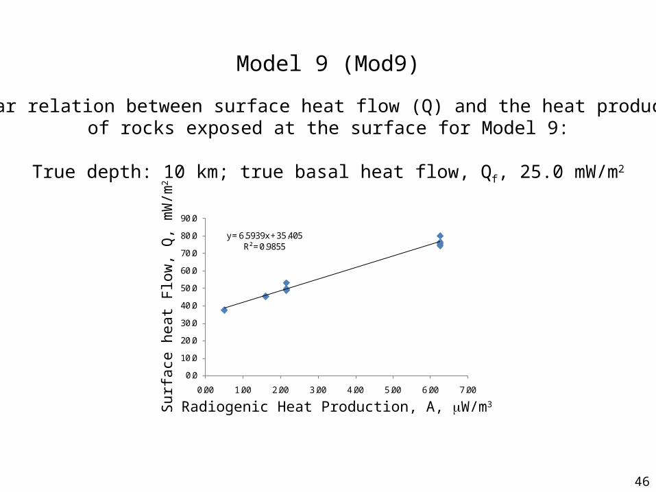
Model 9 (Mod9)
y = 6.5939x + 35.405R² = 0.9855
0.0
10.0
20.0
30.0
40.0
50.0
60.0
70.0
80.0
90.0
0.00 1.00 2.00 3.00 4.00 5.00 6.00 7.00
Radiogenic Heat Production, A, mW/m3
Surf
ace
heat
Flo
w, Q
, mW
/m2
The linear relation between surface heat flow (Q) and the heat production (A)of rocks exposed at the surface for Model 9:
True depth: 10 km; true basal heat flow, Qf, 25.0 mW/m2

47
y = 3.5805x + 23.21R² = 1
20.0
22.0
24.0
26.0
28.0
30.0
32.0
34.0
36.0
38.0
0.00 0.50 1.00 1.50 2.00 2.50 3.00 3.50 4.00
Model 9 (Mod9)
Depth – Slope, km
Inte
rcep
t, m
W/m
2

48
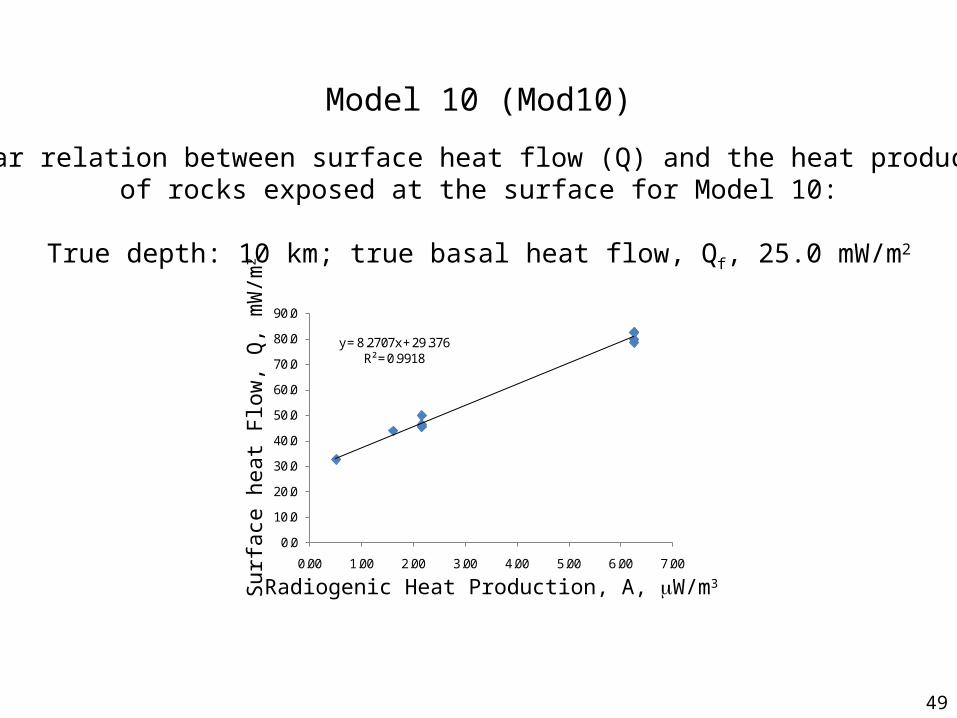
Model 10 (Mod10)
0.00
1.00
2.00
3.00
4.00
5.00
6.00
7.00
0 25 50 75 100 125 150 175 200 225 250
Distance , x direction, kilometers
Hea
t Pro
ducti
on, A
, mW
/m3
2.15 m
W/m
3
6.25 m
W/m
3
1.60 m
W/m
3
0.50 m
W/m
3
2.15 mW/m3
6.25 mW/m3
1.60 mW/m3
0.50 mW/m3
49
y = 8.2707x + 29.376R² = 0.9918
0.0
10.0
20.0
30.0
40.0
50.0
60.0
70.0
80.0
90.0
0.00 1.00 2.00 3.00 4.00 5.00 6.00 7.00
Model 10 (Mod10)
Radiogenic Heat Production, A, mW/m3
Surf
ace
heat
Flo
w, Q
, mW
/m2
The linear relation between surface heat flow (Q) and the heat production (A)of rocks exposed at the surface for Model 10:
True depth: 10 km; true basal heat flow, Qf, 25.0 mW/m2

50
Model 10 (Mod10)
y = 3.5596x + 23.22R² = 1
20.0
22.0
24.0
26.0
28.0
30.0
32.0
0.00 0.25 0.50 0.75 1.00 1.25 1.50 1.75 2.00
Depth – Slope, km
Inte
rcep
t, m
W/m
2
51
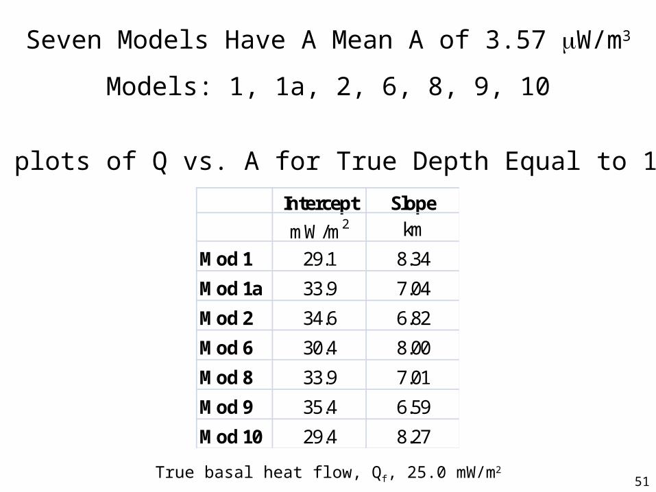
Seven Models Have A Mean A of 3.57 mW/m3
Models: 1, 1a, 2, 6, 8, 9, 10
From plots of Q vs. A for True Depth Equal to 10 kmIntercept SlopemW/m2 km
Mod 1 29.1 8.34
Mod 1a 33.9 7.04
Mod 2 34.6 6.82
Mod 6 30.4 8.00
Mod 8 33.9 7.01
Mod 9 35.4 6.59
Mod 10 29.4 8.27
True basal heat flow, Qf, 25.0 mW/m2

52
Seven Models Have A Mean A of 3.57 mW/m3
Models: 1, 1a, 2, 6, 8, 9, 10
Slope InterceptW/m3 mW/m2
Mod 1 3.57 23.22
Mod 1a 3.59 23.21
Mod 2 3.58 23.21
Mod 6 3.59 23.21
Mod 8 3.58 23.21
Mod 9 3.58 23.21
Mod 10 3.56 23.22
From plots of Intercept vs. Depth – Slope
True basal heat flow, Qf, 25.0 mW/m2

53
The Four Additional Models
Models: 3, 4, 5, 7
From plots of Q vs. A for True Depth Equal to 10 km
Intercept SlopemW/m2 km
Mod 3 37.3 6.20Mod 4 24.9 8.65Mod 5 29.7 7.63Mod 7 28.8 8.46
True basal heat flow, Qf, 25.0 mW/m2

54
The Four Additional Models
Models: 3, 4, 5, 7
From plots of Intercept vs. Depth – Slope
True basal heat flow, Qf, 25.0 mW/m2
Slope InterceptW/m3 mW/m2
Mod 3 3.73 23.13Mod 4 -0.11 25.04Mod 5 2.51 23.74Mod 7 3.65 23.17

55
The Intercept vs. Depth – Slope Relationship
Suggests a Method to Correct for or Model
the Impact of Horizontal Heat Transfer on the
Linear Relationship Between Surface Heat Flow
and Heat Production.

56
Inte
rcep
t, Re
duce
d H
eat F
low
, Q, m
W/m
2
True Depth, b, – Slope (km)
Qf=x1
Qf=x2
Qf=xm
...
n
1ii
n
1iii
width
HPExwidthSlope
57
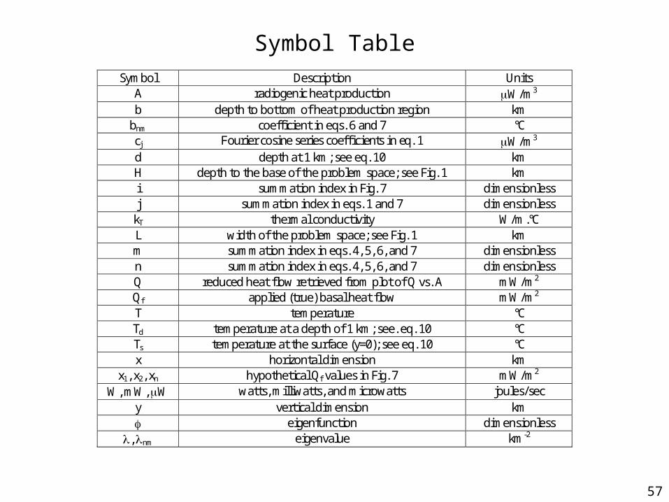
Symbol TableSymbol Description Units
A radiogenic heat production W/m3 b depth to bottom of heat production region km
bnm coefficient in eqs. 6 and 7 °C cj Fourier cosine series coefficients in eq. 1 W/m3 d depth at 1 km; see eq. 10 km H depth to the base of the problem space; see Fig. 1 km i summation index in Fig. 7 dimensionless j summation index in eqs. 1 and 7 dimensionless
kT thermal conductivity W/m.°C L width of the problem space; see Fig. 1 km m summation index in eqs. 4, 5, 6, and 7 dimensionless n summation index in eqs. 4, 5, 6, and 7 dimensionless Q reduced heat flow retrieved from plot of Q vs. A mW/m2 Qf applied (true) basal heat flow mW/m2 T temperature °C Td temperature at a depth of 1 km; see. eq. 10 °C Ts temperature at the surface (y=0); see eq. 10 °C x horizontal dimension km
x1, x2, xn hypothetical Qf values in Fig. 7 mW/m2 W, mW, W watts, milliwatts, and microwatts joules/sec
y vertical dimension km eigenfunction dimensionless
, nm eigenvalue km-2

58
A Comment on the Linear Regressions
• Linear regressions applied using MS Excel® • The Minitab statistical analysis software package• xfitexy.c from Numerical Recipes in C, Press et al.• The method of York and Evensen (2004)• The last 3 methods attempted but not reported
in the present study• Regression method and results require additional
investigation