1

Comprehensive Gasification Modeling of Char Particles with Multi-Modal Pore

Structures

Simcha L. Singer, Ahmed F. Ghoniem*

Department of Mechanical Engineering, Massachusetts Institute of Technology,

77 Massachusetts Ave, Cambridge, MA 02139-4307, USA

Abstract

Gasification and combustion of porous char particles occurs in many industrial

applications. Reactor-scale outputs of importance depend critically on processes that

occur at the particle-scale. Because char particles often possess a wide range of pore sizes

and react under varying operating conditions, predictive models which can account for

the numerous physical and chemical processes and time-dependent boundary conditions

to which a particle is subjected are necessary. A comprehensive, transient, spherically

symmetric model of a reacting, porous char particle entrained in the surrounding flow has

been developed. The model incorporates the adaptive random pore model and consistent

flux relations to account for an evolving, multi-modal pore structure. The model has been

validated against zone II reaction data with good agreement. The framework allows for

concurrent annealing, particle size reduction and the possibility of ash adherence to the

particle surface, although the latter two submodels require the specification of several

parameters. The capability of the model to calculate the evolution of temperature, species

and porosity profiles for char, ash and the surrounding boundary layer has been

demonstrated. The importance of accounting for multiple reactions and for different pore

sizes separately has been illustrated through their effect on overall particle conversion.

Keywords: char; gasification; combustion; porous; particle; random pore model

2

1. Introduction

The gasification behavior of porous char particles is affected by many physical

and chemical processes throughout the course of conversion. Unless the char conversion

occurs at the limit of kinetic control (zone I) or external diffusion control (zone III), some

method of accounting for intra-particle reaction, transport and structural evolution must

be employed to predict burnout behavior. Reactor-level outputs of importance, such as

gas composition and temperature distributions within a gasifier or furnace, overall char

conversion and ash/slag behavior, depend critically on processes that occur at the

particle-scale, necessitating predictive models which can account for the numerous

particle-scale processes and time-varying boundary conditions to which a particle is

subjected. While “global models,” or “effectiveness factor” based models are often used

to predict the conversion of particles tracked within CFD simulations due to

computational limitations, spatially-resolved models of single char particles are useful for

improving the fundamental understanding of the interplay between kinetics, transport and

morphological transformation and also for informing simpler models employed within

CFD settings.

Spatially-resolved models of reacting single char particles in the literature are

numerous, but typically fall into one of two broad categories: models which focus on the

intra-particle transport-reaction-structural coupling and models that focus on processes in

the particle boundary layer, be it complex chemistry [1–5], flow patterns [6–8], or both

[9]. The model described in this paper falls into the former category, so contributions to

that class of model will be discussed briefly, with their salient features, as they pertain to

the model presented in this paper, emphasized.

3

Gavalas employed the random capillary model [10] to predict the porosity and

surface area evolution using the pore growth variable, q, as the equation for local

conversion in a one-dimensional, pseudo-steady state simulation of a multi-modal porous

char particle reacting isothermally with oxygen [11]. A version of the Feng and Stewart

model (FSM) [12] was incorporated into the species equation to model the oxygen flux,

and an equation for the position of the particle surface as the char particle experienced

peripheral fragmentation was derived [11]. Bhatia and Perlmutter incorporated the

random pore model (RPM) [13], which, it can be shown, is equivalent to Gavalas’

random capillary model, into a one-dimensional, pseudo-steady state simulation of a

reacting porous particle [14].

Sotirchos and Amundson [15,16] formulated a general model for transient, one-

dimensional combustion and gasification of porous char, allowing for heterogeneous and

homogeneous reactions and pore-structure-dependent transport and thermodynamic

parameters. The isobaric Dusty Gas Model (DGM [17]) was employed for calculating the

fluxes through the porous particle. An average pore radius for macropores was assumed

to be constant throughout conversion and was used in calculating Knudsen diffusion

coefficients. For both constant radius [15] and shrinking [16] particles, conservation

equations for species, mass and energy were solved within the particle and for a quiescent

boundary layer of thickness equal to the particle’s radius. Ballal et al. incorporated seven

species into a similar framework and studied the effects of reactant concentration on

ignition, quenching and burnout behavior [18]. A later paper by Morell et al. [19] allowed

for pressure buildup within a porous particle, which is a requirement for consistency

between the porous medium fluxes and stoichiometry in a reacting system [20]. While the

4

Dusty Gas expressions for the individual fluxes reduce to the Stefan-Maxwell equations

when the porosity is set to unity (for representation of a gas phase boundary layer), the

DGM expression for the total flux (convective velocity) does not reduce to the correct gas

phase expression.

Reyes and Jensen [21], and later Srinivasachar et al. [22], employed a Bethe

lattice to model the pore structure and used percolation concepts to determine the

effective transport coefficients for an evolving, porous char structure, within a continuum

description of char gasification/combustion. Shrinking from fragmentation was

incorporated, and Srinivasachar et al. employed the Dusty Gas Model to determine the

porous medium fluxes. A mass-transfer coefficient together with an expression for the

non-equimolar fluxes was used as the boundary condition for the species equation at the

char particle surface.

Biggs and Agarwal also employed percolation concepts in a continuum model of

the oxidization of a porous char particle [23]. The Dusty Gas Model was used to calculate

the fluxes, and in the boundary layer within the emulsion phase of a fluidized bed, the

large pore limit of the DGM was employed. The energy equation was also solved in the

particle and the boundary layer.

Wang and Bhatia modeled slow char particle gasification with peripheral

fragmentation, heterogeneous and homogeneous reactions and a bi-disperse Dusty Gas

Model for the porous medium fluxes [24]. The total pressure was allowed to vary within

the particle and the Maxwell-Stefan relations were used to calculate the diffusion fluxes

in the boundary layer. Uniform particle temperature and negligible Stefan flow in the

particle boundary layer were assumed.

5

Zolin and Jensen [25] modified and implemented the annealing model of Suuberg

et al. [26] and Hurt et al. [27] concurrently with a quasi-steady single particle char

oxidation model. Peripheral fragmentation was also incorporated in the model.

Cai and Zygourakis formulated a model for highly porous chars consisting of

spherical cavities (macropores) surrounding microporous, spherical grains [28]. The

species and energy balances for a pseudo-binary mixture were applied to the macropores,

and the reaction source terms, representing consumption of the spherical grains at each

radial location in the char, contained a grain effectiveness factor representing the

Knudsen-diffusion-limited rate of reaction in the microporous grains. The particles were

assumed not to shrink because the high ash content resulted in an ash shell of constant

radius.

Mitchell et al. modeled the oxidation of an isothermal particle using a six step

heterogeneous reaction mechanism [29]. Although not explicitly stated, it appears that the

particle shrinkage was affected in a piece-wise manner by removing the outermost grid-

point once its local conversion was complete.

Many coal and biomass char particles possess multi-modal pore structures which

evolve substantially over the course of conversion in kinetically-limited or mixed

kinetic/intra-particle diffusion-limited conditions. The evolution of the pore structure has

a major effect on the particle’s surface area and on the ability of gaseous reactants to

diffuse through the char structure. It has been shown experimentally that different

reactants have varying degrees of success at penetrating and reacting on micropores and

small mesopores [30–36]. Furthermore, during entrained flow gasification or oxy-

combustion, char particles are subjected to different reactions concurrently or

6

sequentially, meaning that different pore sizes may grow at different rates, affecting the

evolution of the surface area and intra-particle transport processes. In a previous paper,

an adaptive random pore model (ARPM) was developed which extended the original

random pore model to allow different pore sizes to grow at different rates depending on

the instantaneous interplay of kinetics and transport, at the pore scale, at different

locations within a char particle.

This paper incorporates the ARPM into a comprehensive, predictive, single

particle gasification model which is consistent with the evolving, multi-modal pore

structure. Gas transport within the porous structure is modeled using the flux relations of

Feng and Stewart, which together with the ARPM, provide an internally consistent and

predictive method for handling the interplay of transport and pore structure evolution, as

both are based on a geometry consisting of cylindrical capillaries with various radii.

Furthermore, the FSM, explicitly accounts for a pore size distribution, whereas the DGM

employs averaged parameters. The model presented is also comprehensive in nature,

somewhat like a spatially-resolved analogue of the CBK model [27], in that it can

account for concurrent annealing, particle shrinkage (either due to fragmentation or

simply from reaction) and the possibility of ash adherence on the particle surface.

Incorporation of the fragmentation and ash sub-models, however, require some

assumptions and fitting parameters not required by the basic version of the model,

making those sub-models less predictive and more useful as qualitative tools.

7

2. Model Development

2.1 Conservation Equations

To apply a continuum based approach to the modeling of a porous medium, it is

necessary to employ the concept of volume averaging, in which properties are defined as

averages over a representative elementary volume that is larger than the length-scale of

the pores, yet smaller than the characteristic scale of gradients of species, temperature,

etc. Therefore, large voids that appear in cenospheric or sponge-like char particle should

not be treated as pores and included in the averaging [37], but must be handled explicitly

in the particle-scale geometry if a continuum approach is to be employed in a situation

with significant species gradients through the particle. In the context of a one-

dimensional model, a cenospheric particle with a single spherical void at its center can be

treated with the boundary conditions described by Loewenberg and Levendis [38],

however more complex, asymmetric, sponge-like void morphologies would need to be

treated with a full three-dimensional simulation if the continuum approach were to be

applied with fidelity to the actual pore structure.

Aside from the validity of volume averaging, another consideration in applying a

continuum approach is whether the structure has sufficient connectivity for the smooth-

field hypothesis to hold [20]. If the initial porosity or connectivity of the char particle is

below its percolation threshhold, writing partial differential equations for the porous-

medium species and mass conservation is problematic, as discussed by Sahimi et al. [39].

Even above this porosity level, the smooth field approximation is not always valid. These

two limitations must be kept in mind: the connectivity of the porous structure must be

8

sufficient, yet the pores must be small enough to allow for meaningful volume averaging

of properties.

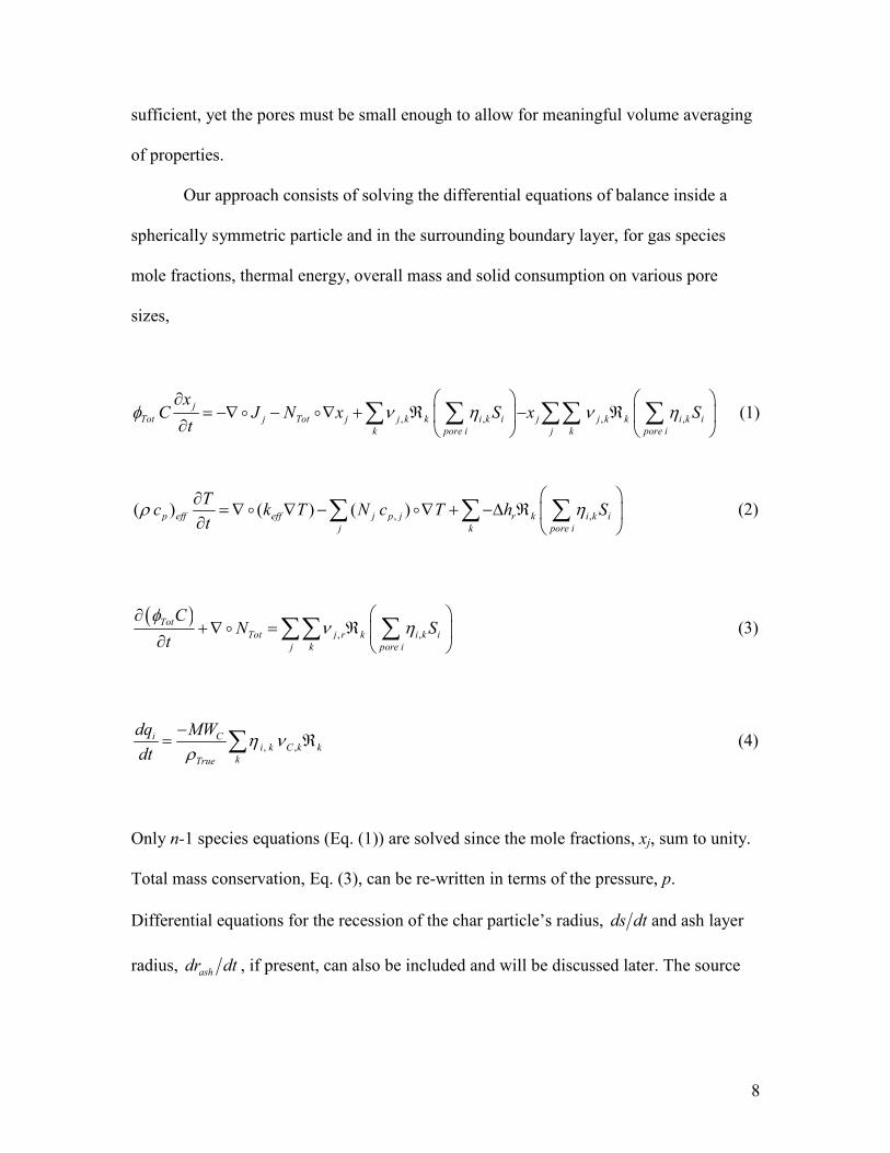
Our approach consists of solving the differential equations of balance inside a

spherically symmetric particle and in the surrounding boundary layer, for gas species

mole fractions, thermal energy, overall mass and solid consumption on various pore

sizes,

, , , ,j

Tot j Tot j j k k i k i j j k k i k i

k pore i j k pore i

xC J N x S x S

tφ ν η ν η

∂ = −∇ − ∇ + ℜ − ℜ

∂ ∑ ∑ ∑∑ ∑� � (1)

, ,( ) ( ) ( )p eff eff j p j r k i k i

j k pore i

Tc k T N c T h S

tρ η

∂= ∇ ∇ − ∇ + −∆ ℜ

∂ ∑ ∑ ∑� � (2)

( ), ,

Tot

Tot j r k i k i

j k pore i

CN S

t

φν η

∂+∇ = ℜ

∂ ∑∑ ∑� (3)

, ,i C

i k C k k

kTrue

dq MW

dtη ν

ρ−

= ℜ∑ (4)

Only n-1 species equations (Eq. (1)) are solved since the mole fractions, xj, sum to unity.

Total mass conservation, Eq. (3), can be re-written in terms of the pressure, p.

Differential equations for the recession of the char particle’s radius, ds dt and ash layer

radius, ashdr dt , if present, can also be included and will be discussed later. The source

9

terms in Eqs. (2.1)-(2.3) contain the factor ,i k i

pore i

Sη ∑ , which represents the pore

surface area (m2C/m3

Tot) participating in a given heterogeneous reaction, k. For

homogeneous reactions this term should be replaced with Totφ (m3gas/m

3Tot), the total

porosity, since homogeneous reaction rates, kℜ , are given in units of (mol/m3gas s)

whereas heterogeneous reaction rates are given in units of (mol/m2C s).

The boundary conditions at the center of the particle, r=0, are dictated by

spherical symmetry,

0, 0, 0jx T p

r r r

∂ ∂ ∂= = =

∂ ∂ ∂. (5a)

The diffusive fluxes, Jj, and total flux, NTot, are also zero at the particle center. Far from

the particle, at r = rbulk, Dirichlet conditions specifying the bulk values of species,

temperature and pressure are imposed,

, ( ), ( ),j j bulk bulk bulkx x t T T t p p= = = . (5b)

At the interface between the porous solid and gas phase, r=s(t), all variables are

continuous, as are all fluxes, with the exception of the heat flux, which is discontinuous

due to radiative exchange between the surface of the particle and the walls or surrounding

gas or particles:

( ) ( )eff s eff s radk T k T q− +− ∇ = − ∇ + . (5c)

10

The boundary conditions may be functions of time to allow for a realistic

representation of the conditions to which a char particle is exposed as it moves through a

reactor. Boundary conditions are not required for the pore growth variables, qi, and the

interface positions at the edge of the char, s, and ash layer, rash (if it exists), since these

are governed by ordinary differential equations. Initial conditions (t=0) for pressure,

temperature and species mole fractions are typically prescribed as uniform profiles, set to

known values if available or simply equal to the initial boundary conditions. The

influence of the initial species mole fraction profiles on the solution fades away very

quickly. Initial values of the pore growth variables are zero and the interface position is

set equal to the initial particle radius, r0.

2.2 Flux Submodels

In addition to determining the surface area available for heterogeneous reactions,

the evolving porous structure also plays a role in the intra-particle species transport.

While the DGM has no way to explicitly account for multi-modal pore structures, the

FSM can be used with any pore size distribution and has the advantage that the adjustable

parameters of the DGM are determined solely by the pore size distribution, given certain

assumptions [12,20]. Essentially, the FSM applies the flux relations of the DGM to a

single pore, and then integrates the given fluxes over all pore sizes and orientations to

calculate the fluxes of each species through the porous medium. This is tractable when

the pore space is assumed to be composed of randomly-oriented, cylindrical capillaries.

The drawbacks of the FSM are its assumption of a thoroughly connected pore structure,

11

which may overestimate the fluxes for low porosities and the assumption that the

equations for long, cylindrical capillaries are valid.

The DGM can be expressed in many different forms [20], one of which separates

the n-1 independent diffusion fluxes, Jj (the sum of the diffusive fluxes is zero), from the

total flux, NTot,

,, ,

, ,

11s j j s j

jss j j s

Kn j eff

s Kn s eff

x J x J xpx p

xRT RT DD

≠

− = − ∇ − − ∇ ∆

∑∑

, (6a)

where,

, , ,, , , ,

, ,

1 1 1

tj s j s effKn s eff Kn j eff

t Kn t eff

xDD D

D

= +∆ ∑

, and (6b)

, , 0

, , , ,

1 1s

s Kn s eff

Tots s

s sKn s eff Kn s eff

J

D B pN p

x xRT

D D

µ

= − − + ∇

∑

∑ ∑. (7)

The effective diffusion coefficients (Knudsen, , ,Kn s effD and continuum, , ,j s effD ) include a

factor which accounts for the total porosity (as well as the tortuosity). This form is

convenient for pairing with the gas boundary layer, in which only n-1 Maxwell-Stefan

12

equations are independent. The diffusive fluxes can be re-written in (n-1) x (n-1) matrix

form as [20]:

1[ ]fJ B RHS−= × , (8)

where,

1, ,

( , )n

j sf

sj n j ss j

x xB j j

=≠

= +∆ ∆∑ , (9a)

, ,

1 1( , )f j

j s j n

B j s x

= − − ∆ ∆ , (9b)

and

, ,

, ,

11j

j js

Kn j eff

s Kn s eff

xpRHS x p

xRT RT DD

= − ∇ − − ∇

∑ (10)

The FSM can also be formulated in terms of the n-1 diffusive fluxes, Jj, and the

total flux, NTot. Under the assumptions of isotropic pore orientation, a pore-size

distribution that can be represented by a number of discrete modes and fully-

interconnected pores, the total smooth field diffusive fluxes are

13

( )11[ ]

3ii f i

pore i

J B RHSφ − = ×

∑ , (11)

and the total flux is given by

,

2, ,

, , , ,

1

83

s i

s Kn s i iTot i i

s spore i pore i

s sKn s i Kn s i

J

D R ppN

x xRT

D D

φ φµ

∇ = − − +

∑∑ ∑

∑ ∑. (12)

For each pore size, i, each of the n-1 terms of iRHS in Eq. (11) is the same as in Eq. (10),

except that the effective terms are replaced by terms specific to each pore size, i, and

( )1/ 3 [ ]i ii f iJ B RHSφ −= × is the vector of diffusion fluxes for all species, s, for each

pore class, i. The Bf -matrices in Eq. (11) are the same as in the case of the DGM (Eq.

(9)), except that the use of effective diffusion coefficients is no longer necessary, since

summations account for each discrete pore size explicitly.

As discussed by Jackson [20] and others [40,41] the development of the FSM

assumes that the smooth field approximation is valid in all pore sizes. This means that the

pore space is thoroughly cross-linked, such that the scalar projection of the smooth field,

particle-scale species gradients in the direction of a pore axis yields the species gradient

in the pore. This is typically satisfied for larger pores, but in the presence of fast

reactions, smooth field concentration gradients may be incorrect for micropores, since the

high surface area to volume ratio implies significant reaction and species gradients along

the micropores, irrespective of their orientation within the particle. The ARPM is useful

14

in approximating when the smooth field assumption breaks down, since pore-scale

effectiveness factors less than unity imply significant gradients along a pore. For

gasification conditions, our simulations generally indicate that the species profiles in

micropores may not satisfy the smooth field assumption, while fluxes in larger pores do

so. For oxidation reactions, micropore concentrations will not satisfy the smooth field

assumption, small mesopores may also fail to do so and it is generally satisfied in larger

mesopores and macropores.

For a first order reaction, Jackson derives a correction factor to apply to pores in

which large pore-scale gradients exist, to be used in conjunction with a smooth-field flux

model [20]. The method solves the same pore scale reaction-diffusion equation used in

deriving the effectiveness factor, but with boundary conditions that account for particle

scale smooth field gradients, and calculates the fluxes through the pore. This method is

not applicable to non-linear reactions. As Jackson has noted, the contribution of the

micropores to the overall flux is, in most cases, small compared with the total flux. This

has been confirmed in our simulations. For this reason, it was deemed safe to neglect the

micropore contribution to the smooth field gas transport.

Finally, as discussed by Gavalas [10] regarding the FSM, it is known that the

assumption of straight, infinite, cylindrical capillaries is not strictly accurate, given the

modest aspect ratio of pores encountered in practice and the fact that much of the pore

volume is overlapped by more than one pore, especially later in conversion. While this is

not a problem in terms of assigning the porosities in the context of the random pore

model, it does alter the idealized geometry on which the FSM is based. For this reason,

similar to the bi-disperse DGM developed in [24], in place of the pore radius, Ri, in the

15

FSM we have employed a hydraulic radius for each pore size: , 2 /h i i ir Sφ= . This is used

in Eq. (12) and in calculating diffusion coefficients (Section 3.2) for use in Eqs. (10)-

(12).

In the surrounding gas film in which the char particle is entrained, mass transfer

occurs via continuum diffusion and radial convection due mainly to Stefan flow (the net

creation of gas molecules from heterogeneous reactions). The Maxwell-Stefan equations

can be solved for the diffusive fluxes of n-1 species, where it has been assumed that

pressure gradients in the boundary layer are negligible:

,

s j j s

j

s j s

x J x J px

D RT

−= − ∇∑ (13)

The nth diffusive flux can be obtained from the constraint that the fluxes sum to zero. Eq.

(13) can also be written in matrix form,

1[ ]fJ B RHS−= × (14a)

1, ,

( , )n

j sf

sj n j ss j

x xB j j

D D=≠

= +∑ (14b)

, ,

1 1( , )f j

j s j n

B j s xD D

= − −

(14c)

j j

pRHS x

RT= − ∇ (14d)

16

The radial velocity in the boundary layer is calculated from Eq. (3), since total

pressure is almost constant outside the particle and a separate equation for the gas phase

momentum is not necessary. Within the particle, Eq. (3) is used to calculate the pressure,

since pressure may build up within the porous structure.

2.3 Pore Structure Evolution Submodel

Since non-catalytic gas-solid reactions occur on surfaces, the amount of surface

area available for reaction will directly affect the rate of solid conversion. For most chars,

the internal surface area is orders of magnitude larger than the external surface area and

this internal area may change substantially throughout conversion. The random pore

models assume that the pore space consists of randomly located and oriented (and

therefore overlapping) cylindrical capillaries [10,13]. Any distribution of pore radii is

acceptable, so the random pore models have great flexibility in matching experimental

data. Due to their simplicity, flexibility and success at reproducing experimental data

stemming from their ability to account for pore growth and overlap, the random pore

models have become the most widely used models for pore structure evolution in non-

catalytic gas-solid reactions.

The adaptive random pore model (ARPM) extends the original random

capillary/pore models ([10,13]) to situations in which different pore sizes may grow at

different rates due to instantaneous, pore scale diffusion limitations at different locations

within a char particle, and is adopted to model the evolution of the pore structure [42].

Many researchers, using different techniques, have shown that different gases react to

varying extents on certain pore sizes, even in the “kinetically controlled” regime [30–36].

17

For a situation in which multiple reactants are present simultaneously and in which intra-

particle diffusion limitations result in species gradients throughout a char particle,

different locations in a particle may experience growth on a different range of pore sizes.

Relevant examples of this situation could be entrained flow gasification and oxy-fuel

combustion, in which multiple reactants are present and the char is exposed to time-

dependent boundary conditions in both cases.

Like the original RPM, the ARPM is a predictive model (with the possible

exception of some diffusion parameters), once the original pore size distribution has been

measured and discretized. It is emphasized that both the ARPM and the original RPM

require knowledge of the pore size distribution if the model is to be used in a predictive

manner. (To get the RPM parameter,ψ , it is necessary to calculate the total length of

pores, which requires the pore size distribution.) The ARPM is used to predict the

porosity, surface area and radii of the various pore sizes as the particle reacts in any

regime. The equations representing the ARPM are based on the discrete form of Gavalas’

derivation [11]. The pore size distribution of the char is measured and the pore sizes

divided into bins of initial porosity, 0,iφ , and radius, 0,iR . The random pore geometry

implies that the length of pore axes per unit volume, for each pore size, is given by [11]:

0,1

0, 20,

0,

11

ln

1

n

j

j i

i n

ij

j i

lR

φ

π φ

= +

=

−

= −

∑

∑. (15)

The individual and total porosities are given, at any conversion, by [11]:

18

2 20, 0,

1

1 exp( ) exp( )n

i i i j j

j i

l R l Rφ π π= +

= − − − ∑ (16a)

20,

1

1 exp( )n

Tot j j

j

l Rφ π=

= − − ∑ . (16b)

In the ARPM, each pore size grows by an amount qi(t), and therefore at any time, the

radius of pore size i, is given by [42],

0,i i iR R q= + . (17)

The growth of each pore size is due to reaction on its surface, and is given by the “state

equations” for the solid phase, Eq. (4),

, ,i C

i k C k k

kTrue

dq MW

dtη ν

ρ−

= ℜ∑ , (4)

where n

k k kk pℜ = is the intrinsic heterogeneous reaction rate and ,i kη is the pore-scale

effectiveness factor for pore size i and reaction k. The expressions for the pore-scale

effectiveness factor are approximations based on classical Thiele theory and the geometry

of the random pore system, and are given in the appendix. The surface area associated

with pores of size i, is given by [42],

19

( ) 0, 0,1 2 ( )j Toti Tot i i i

j i i

S l R qq q

φ φφ π

∂ ∂= = = − +

∂ ∂∑ . (18)

Although it is not required to calculate the pore structure evolution, the conversion rate

on each pore size is given by,

,

0,(1 )True i i i

Tot

dX S dq

dt dtφ=

−, (19)

and the amount of conversion due to reaction on each pore size, , ( , )True iX r t is given by

numerical integration [42]:

',

0, 0

1( )

(1 )

iq

True i i i i

Tot

X q S dqφ

=− ∫ . (20)

2.4 Reaction Submodels

The single particle model in this paper considers both heterogeneous and

homogeneous reactions. The question of whether homogeneous reactions occur within

the pore space (or within certain pore sizes) or only in the boundary layer appears to be

unresolved, but in any case, it is a simple matter to modify the model one way or the

other. In this study, homogeneous reactions have been confined to the particle boundary

layer. As the model focuses on the interplay between transport, kinetics and pore

structure evolution, species equations for surface or gas phase intermediates are not

considered. Therefore, adsorption/desorption mechanisms which assume the

20

intermediates to be in pseudo-steady state, like Langmuir-Hinshelwood expressions,

could be incorporated, but detailed kinetic mechanisms for gas-phase or solid phase

reactions are not included in the modeling framework at this time. Up to six gaseous

species may be present (in this paper: O2, H2, H2O, CO, CO2 and N2), with three

heterogeneous (R1-R3) and two homogeneous (R4, R5) reactions considered in this

paper:

2 2C CO CO+ → (R1)

2 2

2 1

2( 1) 1 1C O CO CO

ξ ξξ ξ ξ+

+ → ++ + +

(R2)

2 2C H O CO H+ → + (R3)

2 21

2CO O CO+ → (R4)

2 2 21

2H O H O+ → (R5)

The expression for homogeneous reaction (R4) is from [43] and that of (R5) is

taken from [44]. For simplicity, in this paper, nth order heterogeneous reactions are

considered. For carbon oxidation, nth order behavior has been explained as being a

consequence of the distribution of activation energies for combustion among the carbon

sites [45]. Although gasification reactions (R1) and (R3) have been shown experimentally

to be best represented by Langmuir-Hinshelwood forms, in this paper, which focuses on

model development and validation under low pressure conditions, the power law form

has been employed. A final issue needing clarification is the CO/CO2 ratio formed by

21

reaction (R2). The results of Tognotti et al. [46] for Spherocarb oxidation have been

adopted which gives,

( )70exp 3070 Tξ = − . (21)

2.5 Annealing

Annealing is a high temperature process that reduces the reactivity of solid fuel

particles. It is thought to be caused by an increase in atomic ordering of the carbon

matrix, similar to the process of graphitization. Annealing has been shown to reduce the

reactivity of an un-annealed char by up to two orders of magnitude [47], with potentially

even greater reductions [27]. The annealing model originally developed by Suuberg et al.

[26] with subsequent modifications [27,47] has been applied in this study. This model is

able to describe the experimentally observed rapid reduction and subsequent plateau in

reactivity when a char is subjected to an isothermal heat treatment, as well as the

observation that the activation energy for annealing increases for higher temperature heat

treatments [27]. The interpretation of these observations is that fresh char contains active

sites with a distribution of activation energies for annealing, Ed. Initially, the char

undergoes rapid atomic rearrangements upon heating, but as the lower activation energy

rearrangements proceed toward completion, further solid-phase transformations require

ever higher temperatures. Hurt et al. employed a log-normal distribution for the initial

annealing activation energies [27], while Zolin et al. used a shifted gamma distribution

based on experiments performed with a variety of chars [47].

22

The initial normalized distribution of active sites, F, as a function of annealing

activation energies, Ed, is a shifted gamma function.

1( ) ( )( , 0) exp

( )d d

d

E EF E t

α

α

δ δα β β

−− − = = − Γ

(22)

Annealing destroys active sites as a first order process in the remaining active sites, for

each activation energy,

expd

dd

E

F EA F

RTt

∂ − = − ∂ . (23)

This equation can be integrated, using the initial distribution of active sites, to yield the

updated, normalized distribution of activation energies,

1( ) ( )( , ) exp exp exp

( )d d d

d d

E E EF E t A t

RT

α

α

δ δα β β

−− − − = − − Γ . (24)

The fraction of active sites remaining at any time, N(t)/N0, is obtained by integration over

all activation energies:

0 0

( )( )d d

N tF E dE

N

∞

= ∫ . (25)

23

The char’s post-heat treatment reactivity towards O2, CO2, etc. at any time, kHT, is the

original, un-annealed reactivity, k0, multiplied by the fraction of active sites remaining,

N(t)/N0,

0

0

( )HT

N tk k

N= . (26)

The same formulation may be used whether the heat treatment is isothermal, or as is the

case in practice, when the temperature varies significantly with time. Although not stated

explicitly [25], this may be handled by dividing the temperature-time history into discrete

time bins (of duration tbin) of uniform temperature (Tbin), and applying Eq. (23) to each

time bin. The initial condition for each bin is the distribution function F(t, Ed) where t is

now the time at the end of the previous bin. This continues for each temperature-time bin,

giving the following equation, which replaces Eq. (24), for the fraction of active sites

remaining at a given time:

1( ) ( )( , ) exp exp exp

( )d d d

d d bin

bin bin

E E EF E t A t

RT

α

α

δ δα β β

− − − −= − − Γ ∑ , (27)

which can be integrated over all activation energies, Ed, to obtain kHT.

2.6 Peripheral Fragmentation and Ash Behavior

Fragmentation of coal chars during conversion has been observed or inferred by

several investigators (e.g., [48–50]). While fragmentation during devolatilization can be

24

caused by pressure buildup within the particle, during char consumption in furnaces or

entrained flow gasifiers, fragmentation is thought to be a percolation phenomenon, in

which the char disintegrates due to a loss of structural integrity at a critical value of

connectivity or porosity. Not all chars fragment during conversion. Whether a particular

char will fragment cannot be easily predicted, although it depends on the distribution of

pore sizes, its ash content and temperature.

When an initially uniform, isothermal porous particle reacts under purely kinetic

control, percolative fragmentation should occur simultaneously throughout the particle,

but when species gradients are present and the particle is consumed faster near its edge

than near the particle center, the critical porosity is reached first near the particle surface.

This is referred to as perimeter or peripheral fragmentation and in this case a

fragmentation front moves from the outer part of the particle inwards, causing the particle

to shrink as the critical porosity is achieved at progressively smaller radial locations [11].

While percolative fragmentation is actually a discrete phenomenon, with a distribution of

finite particle sizes [51], it can be modeled using an equation for a continually moving

particle radius, since the fragments are quite small for the case of perimeter fragmentation

[50]. There are two stages to the particle’s size evolution. Prior to the outermost volume

of the particle achieving the critical porosity, i.e. when 0( , ) criticalr tφ φ< , the recession of

the particle radius due to reaction on the external surface is minimal [10,11]. Once the

critical porosity is reached at the outermost section, an equation for the particle radius is

obtained by taking the total time derivative of ( ( ), ) criticalr s t tφ φ= = , which yields [11]:

0d ds

dt r dt t

φ φ φ∂ ∂= + =∂ ∂

, (28)

25

which can be rearranged to give,

0

( )

0 ( , )

( ( ), )

critical

critical

r R t

if s r t

dst if s t tdt

r

φ φ

φ

φ φφ

=

= < ∂

= ∂− = ∂ ∂

. (29)

This is the differential equation for the rate of recession of the particle surface in the case

of peripheral fragmentation. Char, as well as any ash contained therein, is liberated and

assumed to react quickly away from the particle.

Not all chars exhibit fragmentation during reaction in regime I or II. While the

reasons for this are not known, one possibility for the absence of fragmentation is the

presence of ash. For some high ash chars reacting at temperatures below ash melting, it is

possible that a solid ash shell remains surrounding a carbon rich core, causing the particle

to maintain its original size. However, in many practical cases, the temperature of the

particle is such that the included ash will become soft, sticky or melted. It is possible that

the presence of sticky ash inclusions prevent the char from fragmenting. In such a case,

the ash particles would not be liberated once local conversion reaches unity, but rather,

isolated particles would adhere to the receding char particle surface [52], possibly

contributing to an increased resistance to gas transport late in the particle’s conversion

[27].

In modeling such a case, there are essentially three stages to the evolution of the

particle size, rather than the two that exist for the case of peripheral fragmentation.

26

During the first stage, the particle’s radius is constant since while its outermost volume

hasn’t been fully converted. Once porosity at the particle edge reaches a value

approaching 100%, the particle begins to shrink with ash particles adhering to the

surface. These two stages are identical, mathematically, to the two stages that exist for

peripheral fragmentation, with the only difference being that in the case of ash adherence,

the “critical porosity” is closer to unity. During the second stage the ash particles are

assumed to be too few in number to affect the transport of gas to and from the porous

matrix.

Once the particle’s surface has receded enough to liberate a “critical volume” of

ash, a continuous ash layer is formed [27]. There are now three separate regions in the

computational domain: porous char, porous ash and a gas-phase boundary layer. Due to

the process of ash melting/sintering, the porosity of the ash layer may decrease in time.

Since the outermost portion of the ash layer has been exposed and free to coalesce for

longer than portions nearer to the char surface, the porosity of the ash layer may also be a

function of position. Once the porosity anywhere within the ash layer decreases below the

percolation threshold, it is assumed that all reactions cease and the remaining char has

been encapsulated inside the ash.

Loewenberg and Levendis [38] calculated the extent of the ash layer, rash(t), using

a balance on the mineral matter contained in the char and the instantaneous char radius,

s(t). A balance on the mineral matter in the char that allows the ash layer porosity to vary

with position, assuming none is lost to vaporization, yields

( )

3 3 20

( )

( ) 3 (1 ( , ))ashr t

ash ash ash

s t

r f s t f r r t drφ= + −∫ . (30)

27

The quantity of interest is rash(t), which only appears in the upper limit of the integral in

Eq. (30). Taking the time derivative of both sides and using the Leibnitz rule on the

integral gives

( )

2 2 2 2

( )

(1 ( , ))(1 ( , )) (1 ( ( ), ))

ashr t

ash ashash ash ash ash ash

s t

r t drds dsf s r dr r r t s s t t

dt t dt dt

φφ φ

∂ −− = + − − −

∂∫ (31)

It will be assumed that the local porosity of the ash layer is a linearly decreasing function

(with rateϒ ) of the time that the ash is both above the softening temperature and exposed

on the surface of the char, which can be represented using a sigmoid function

[ ],0

_ exp ( )

( , )1 exp 10( )

t

ash ash

ash meltt osed r

dtr t

T Tφ φ= − ϒ

+ − −∫ . (32)

If the ash temperature is assumed to be uniform, typically a good assumption, the

integrand in Eq. (31) is only a function of Tash(t) and is independent of position. It can

therefore be brought outside the integral, which is now easily evaluated. Equation (31)

can be rearranged to give an equation for the ash layer thickness as a function of the char

particle radius, its time derivative and the rate at which the ash is decreasing in porosity:

( )( )

( )[ ]

3 3

2

2

( ) ( )( ) 1 ( ( )

3 1 exp[ 10( )]

( ) 1 ( ( ))

ash

ash ash

ash meltash

ash ash ash

r t s tdss t s t f

dt T Tdr

dt r t r t

φ

φ

−ϒ− − − + − −

=−

. (33)

28

Equations (32) and (33) are the equations governing ash layer behavior

incorporated in the model. Unless there is a discontinuity in the value of the ash porosity

at the char/ash interface, then the first term in the numerator of Eq. (33) is zero. Note that

the linear rate of decrease in ash porosity is simplistic, not least due to the fact that the

porosity obviously levels off as it approaches zero. However it is necessary for a tractable

solution, because other forms would not allow the integral in Eq. (31) to be evaluated

analytically. Also note that the entire reaction ceases when the porosity anywhere in the

ash layer reaches some minimum (percolation) threshold. This is physically plausible as

well as necessary to maintaining Eq. (31) independent of r. This also somewhat alleviates

the problem of a linear rate being unrealistic near a porosity of zero, since the porosity

would never approach zero before reactions have ceased.

Finally, gas diffusion through the ash layer must be described. The dusty gas

model approach is adopted (FSM with a single pore size) with an average pore size given

by the hydraulic radius, 2 /ash ash ashR Sφ= . The porosity of the ash is given by Eq. (32)

and the surface area of the ash has been taken as constant but could easily be made a

function of ashφ and information on ash particle size.

3. Numerical Approach

3.1 Numerical Implementation

Because of the highly non-linear and stiff nature of the system of governing

equations, a method of lines approach has been adopted in order to take advantage of the

sophisticated computational tools that have been developed for solving large systems of

29

ordinary differential equations (ODEs). The partial differential equations (Eqs.(1)-(3))

are transformed into a set of ODEs using the well-known finite volume discretization

along the spatial coordinate. The resulting system of ODEs is then integrated in time

using a fully implicit scheme, with a Jacobian-free Newton-Krylov method employed for

the solution of the resulting system of nonlinear algebraic equations at each time step. At

each nonlinear Newton iteration, the iterative GMRES method is employed to solve the

resulting linear system without having to evaluate the Jacobian. Banded preconditioning

matrices were applied from the left. The code was written in MATLAB and the temporal

integration described above was performed using the CVODE solver [53]. The typical

relative tolerance was 10-5 and absolute tolerances of 10-6 were used for variables that

were of order unity.

The physical domain was discretization using the control volume formulation

employed by Patankar [54], with an non-uniform grid generated using general interior

stretching functions [55]. The non-uniform grid allows for increased resolution in areas

of steep gradients, such as near the particle/gas phase interface. All state variables were

calculated at the control volume centers, with the exception of the velocity in the gas

phase, which was calculated at the control volume faces. Similarly, all diffusion and

convective fluxes were evaluated at the control volume faces. All advective terms were

evaluated using upwinding. The domain typically extended to 10 particle radii.

The multi-component fluxes are evaluated at the control volume faces using the

Feng and Stewart model within the particle and using the Maxwell-Stefan multi-

component diffusion relations in the gas phase. The state variables required by these flux

models are calculated using linear interpolation between the adjacent grid point values.

30

The transport coefficients required by these flux models corresponding to

“conductivities” (e.g. Dj, Dj,s) are functions of temperature, mole fraction, pore size, etc.,

and are evaluated using harmonic averaging of the surrounding grid points. The harmonic

mean provides a convenient and physically realistic method of accounting for instances

of sharp transition of properties, which are especially pronounced at the interface

between the porous solid and the homogeneous gas phase in which pore size and

Knudsen diffusivities become infinite [54]. It should be noted that taking the harmonic

mean of the entire matrix of coefficients 1[ ]fB − may result in discontinuities; therefore,

the harmonic mean of the individual components of the matrices should be calculated.

At the particle/gas-phase interface there is an additional heat flux due to radiative

exchange between the surface of the char particle and its surroundings. Using two

infinitesimal control volumes at the interface, one can derive, from Eq. (5c), a non-linear

algebraic expression for the interface temperature in terms of the temperatures on either

side of the interface and the temperature with which the particle interacts radiantly. This

non-linear equation cannot be solved explicitly for the interface temperature, Ts. Solving

a non-linear algebraic equation would necessitate either solving the model as a

differential algebraic system or employing a non-linear equation solving routine at every

time step of the ODE solver; both of which are undesirable. Therefore, the non-linear

term on the right-hand side is lagged by one time-step to give an explicit equation for the

current interface temperature. A similar procedure is adopted in solving for the pore-scale

effectiveness factors that appear in Eq. (A2) via Eq. (A3), in that the effectiveness factor

terms that appear on the right-hand side of Eq. (A3) are lagged by one time-step. Since

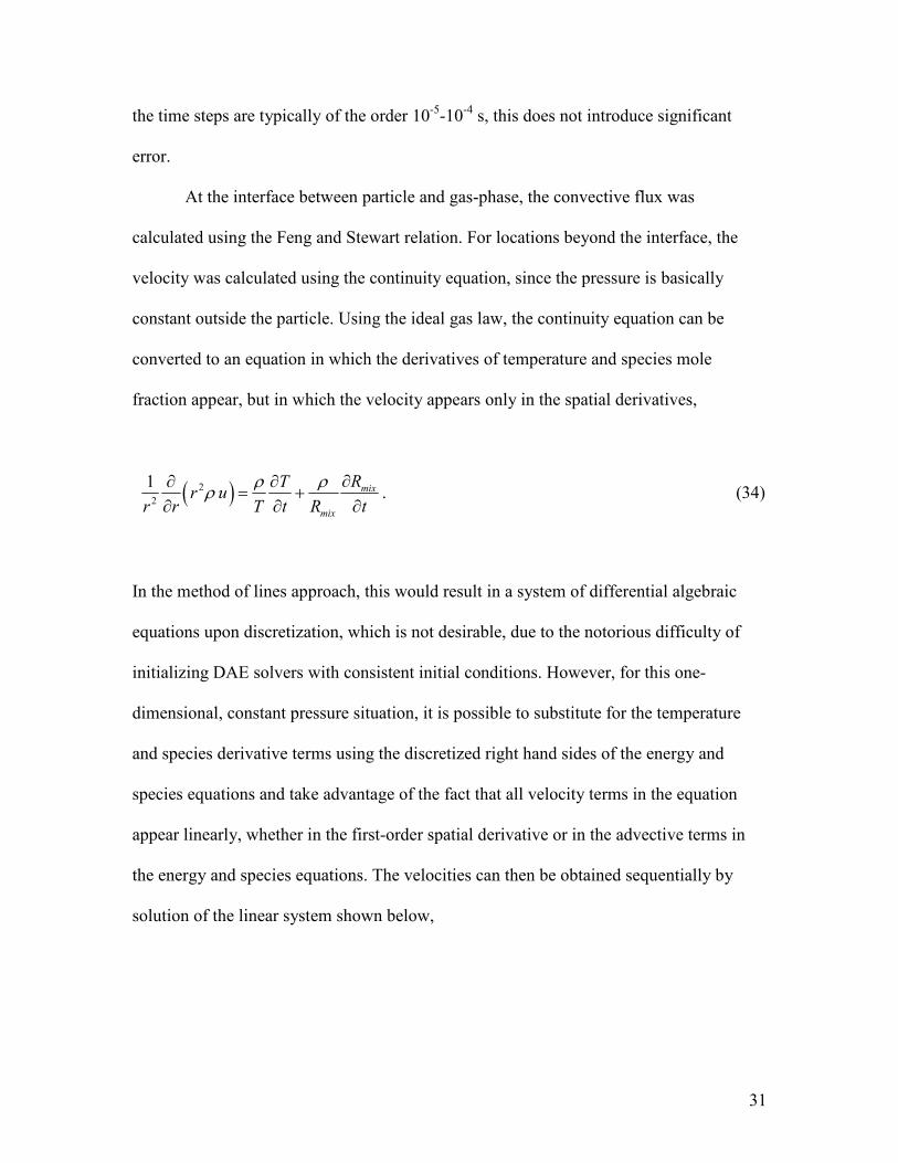
31

the time steps are typically of the order 10-5-10-4 s, this does not introduce significant

error.

At the interface between particle and gas-phase, the convective flux was

calculated using the Feng and Stewart relation. For locations beyond the interface, the

velocity was calculated using the continuity equation, since the pressure is basically

constant outside the particle. Using the ideal gas law, the continuity equation can be

converted to an equation in which the derivatives of temperature and species mole

fraction appear, but in which the velocity appears only in the spatial derivatives,

( )2

2

1 mix

mix

RTr u

r r T t R t

ρ ρρ

∂∂ ∂= +

∂ ∂ ∂. (34)

In the method of lines approach, this would result in a system of differential algebraic

equations upon discretization, which is not desirable, due to the notorious difficulty of

initializing DAE solvers with consistent initial conditions. However, for this one-

dimensional, constant pressure situation, it is possible to substitute for the temperature

and species derivative terms using the discretized right hand sides of the energy and

species equations and take advantage of the fact that all velocity terms in the equation

appear linearly, whether in the first-order spatial derivative or in the advective terms in

the energy and species equations. The velocities can then be obtained sequentially by

solution of the linear system shown below,

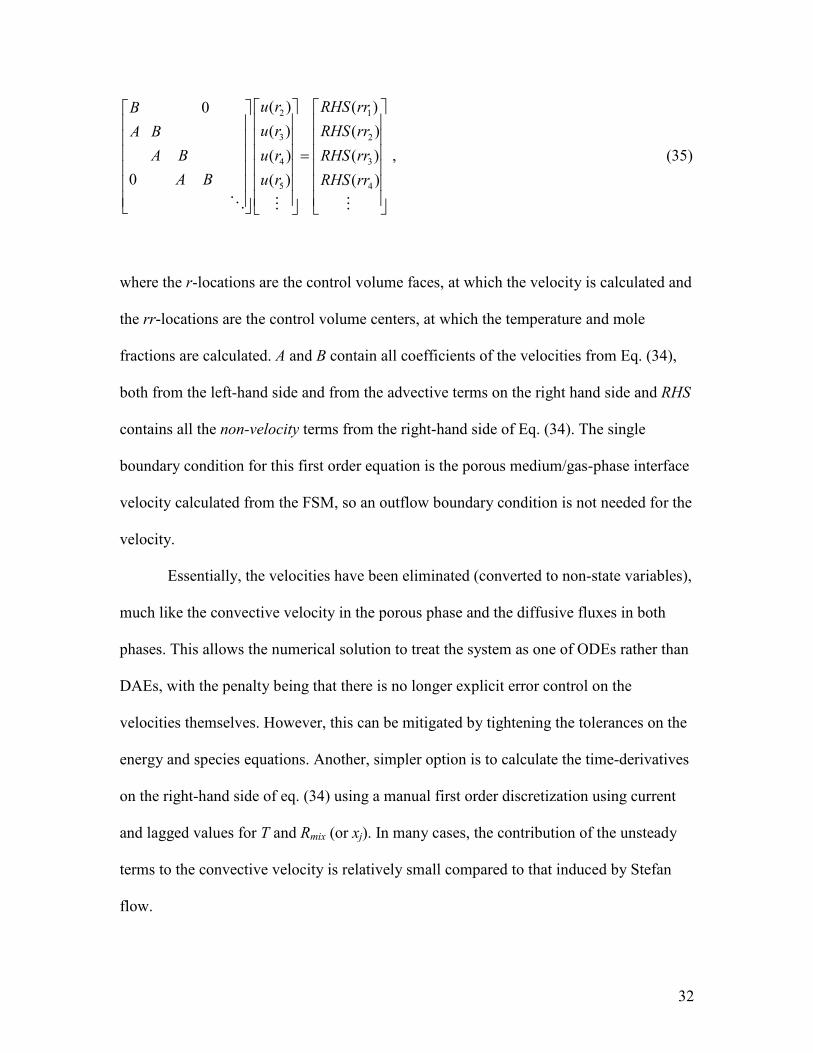
32

2 1

3 2

4 3

5 4

( ) ( )0

( ) ( )

( ) ( )

0 ( ) ( )

u r RHS rrB

u r RHS rrA B

A B u r RHS rr

A B u r RHS rr

= ⋱ ⋮ ⋮

, (35)

where the r-locations are the control volume faces, at which the velocity is calculated and

the rr-locations are the control volume centers, at which the temperature and mole

fractions are calculated. A and B contain all coefficients of the velocities from Eq. (34),

both from the left-hand side and from the advective terms on the right hand side and RHS

contains all the non-velocity terms from the right-hand side of Eq. (34). The single

boundary condition for this first order equation is the porous medium/gas-phase interface

velocity calculated from the FSM, so an outflow boundary condition is not needed for the

velocity.

Essentially, the velocities have been eliminated (converted to non-state variables),

much like the convective velocity in the porous phase and the diffusive fluxes in both

phases. This allows the numerical solution to treat the system as one of ODEs rather than

DAEs, with the penalty being that there is no longer explicit error control on the

velocities themselves. However, this can be mitigated by tightening the tolerances on the

energy and species equations. Another, simpler option is to calculate the time-derivatives

on the right-hand side of eq. (34) using a manual first order discretization using current

and lagged values for T and Rmix (or xj). In many cases, the contribution of the unsteady

terms to the convective velocity is relatively small compared to that induced by Stefan

flow.

33

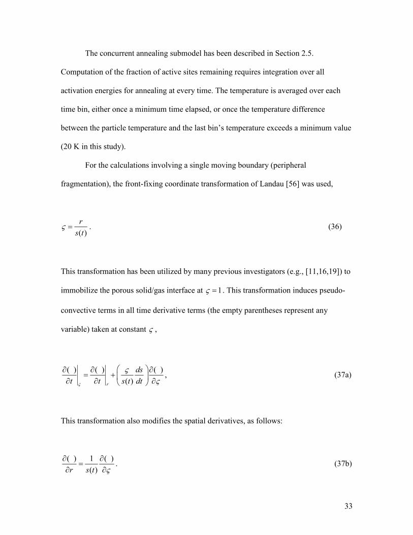
The concurrent annealing submodel has been described in Section 2.5.

Computation of the fraction of active sites remaining requires integration over all

activation energies for annealing at every time. The temperature is averaged over each

time bin, either once a minimum time elapsed, or once the temperature difference

between the particle temperature and the last bin’s temperature exceeds a minimum value

(20 K in this study).

For the calculations involving a single moving boundary (peripheral

fragmentation), the front-fixing coordinate transformation of Landau [56] was used,

( )

r

s tς = . (36)

This transformation has been utilized by many previous investigators (e.g., [11,16,19]) to

immobilize the porous solid/gas interface at 1ς = . This transformation induces pseudo-

convective terms in all time derivative terms (the empty parentheses represent any

variable) taken at constant ς ,

( ) ( ) ( )

( )r

ds

t t s t dtς

ςς

∂ ∂ ∂= + ∂ ∂ ∂

, (37a)

This transformation also modifies the spatial derivatives, as follows:

( ) 1 ( )

( )r s t ς∂ ∂

=∂ ∂

. (37b)

34

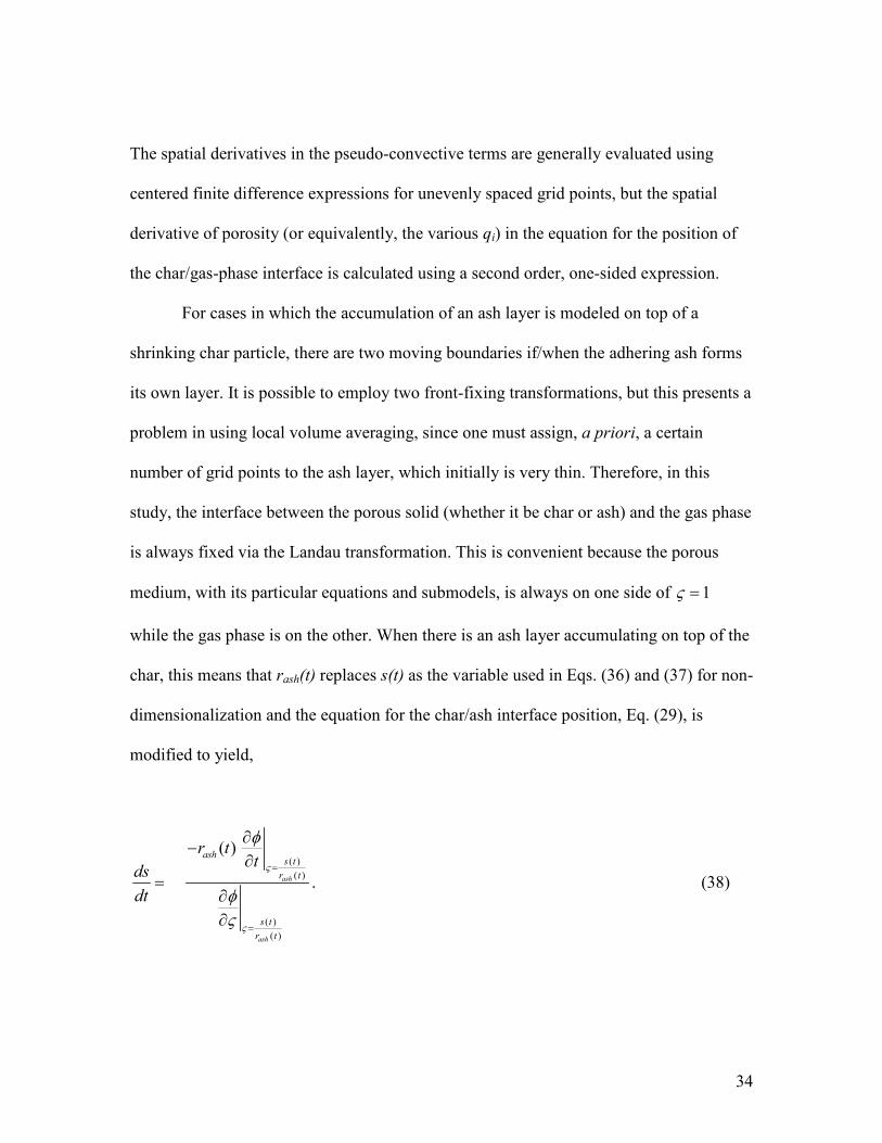
The spatial derivatives in the pseudo-convective terms are generally evaluated using

centered finite difference expressions for unevenly spaced grid points, but the spatial

derivative of porosity (or equivalently, the various qi) in the equation for the position of

the char/gas-phase interface is calculated using a second order, one-sided expression.

For cases in which the accumulation of an ash layer is modeled on top of a

shrinking char particle, there are two moving boundaries if/when the adhering ash forms

its own layer. It is possible to employ two front-fixing transformations, but this presents a

problem in using local volume averaging, since one must assign, a priori, a certain

number of grid points to the ash layer, which initially is very thin. Therefore, in this

study, the interface between the porous solid (whether it be char or ash) and the gas phase

is always fixed via the Landau transformation. This is convenient because the porous

medium, with its particular equations and submodels, is always on one side of 1ς =

while the gas phase is on the other. When there is an ash layer accumulating on top of the

char, this means that rash(t) replaces s(t) as the variable used in Eqs. (36) and (37) for non-

dimensionalization and the equation for the char/ash interface position, Eq. (29), is

modified to yield,

( )

( )

( )

( )

( )

ash

ash

ashs t

r t

s t

r t

r tt

ds

dt

ς

ς

φ

φς

=

=

∂−

∂=

∂∂

. (38)

35

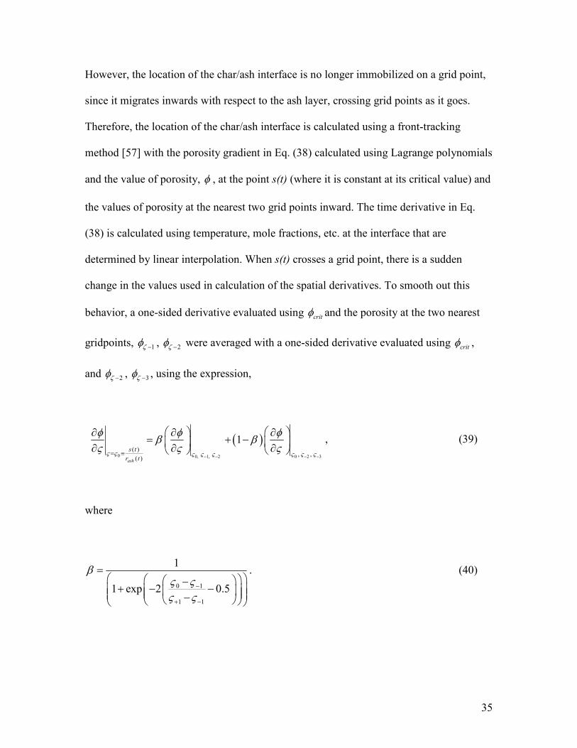
However, the location of the char/ash interface is no longer immobilized on a grid point,

since it migrates inwards with respect to the ash layer, crossing grid points as it goes.

Therefore, the location of the char/ash interface is calculated using a front-tracking

method [57] with the porosity gradient in Eq. (38) calculated using Lagrange polynomials

and the value of porosity, φ , at the point s(t) (where it is constant at its critical value) and

the values of porosity at the nearest two grid points inward. The time derivative in Eq.

(38) is calculated using temperature, mole fractions, etc. at the interface that are

determined by linear interpolation. When s(t) crosses a grid point, there is a sudden

change in the values used in calculation of the spatial derivatives. To smooth out this

behavior, a one-sided derivative evaluated using critφ and the porosity at the two nearest

gridpoints, 1ζφ − , 2ζφ − were averaged with a one-sided derivative evaluated using critφ ,

and 2ζφ − , 3ζφ − , using the expression,

( )0 0, 1, 2 0 2 3

( ), ,

( )

1

ash

s t

r tς ς ς ς ς ς ς ς

φ φ φβ β

ς ς ς− − − −= ≡

∂ ∂ ∂= + − ∂ ∂ ∂

, (39)

where

0 1

1 1

1

1 exp 2 0.5

βς ςς ς

−

+ −

= −+ − − −

. (40)

36

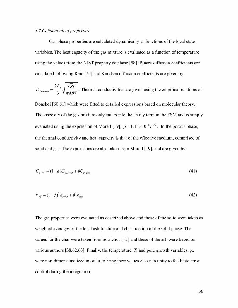
3.2 Calculation of properties

Gas phase properties are calculated dynamically as functions of the local state

variables. The heat capacity of the gas mixture is evaluated as a function of temperature

using the values from the NIST property database [58]. Binary diffusion coefficients are

calculated following Reid [59] and Knudsen diffusion coefficients are given by

2 8

3i

Knudsen

R RTD

MWπ= . Thermal conductivities are given using the empirical relations of

Donskoi [60,61] which were fitted to detailed expressions based on molecular theory.

The viscosity of the gas mixture only enters into the Darcy term in the FSM and is simply

evaluated using the expression of Morell [19], 5 1/21.13 10 Tµ −= × . In the porous phase,

the thermal conductivity and heat capacity is that of the effective medium, comprised of

solid and gas. The expressions are also taken from Morell [19], and are given by,

, , ,(1 )p eff p solid p gasC C Cφ φ= − + (41)

2 2(1 )eff solid gask k kφ φ= − + (42)

The gas properties were evaluated as described above and those of the solid were taken as

weighted averages of the local ash fraction and char fraction of the solid phase. The

values for the char were taken from Sotrichos [15] and those of the ash were based on

various authors [38,62,63]. Finally, the temperature, T, and pore growth variables, qi,

were non-dimensionalized in order to bring their values closer to unity to facilitate error

control during the integration.

37

4. Results and Discussion

To test the single particle char consumption model without using fitting

parameters, it is necessary to have, as input, measurements of the char’s pore size

distribution, particle size, density and ash content, as well as zone I reaction rate data at a

conversion level at which the pore size distribution has also been measured [42]. For

purposes of validation, zone II measurements of interest such as conversion, temperature,

diameter or surface area vs. time, for the same char, must be available, together with the

boundary conditions to which the particle has been exposed throughout its conversion.

We have attempted to validate the model with zone II Spherocarb oxidation data

from the literature [64,65]. Spherocarb, a synthetic char, has been employed by several

research groups for fundamental studies of char gasification and oxidation. Its pore

structure has been well characterized, it contains minimal amounts of ash, a small amount

of remaining volatiles and moisture (~4% wt), is highly spherical and remains so with

conversion [65] and is of uniform size (diameter of 140 µm with a standard deviation of 9

µm [64]), making it highly suitable for validation of the model. The initial pore structure

of Spherocarb and its reaction rate with oxygen in the kinetically controlled regime has

been characterized extensively and is summarized by D’Amore, et al. [66–68]. The pore

size distributions presented therein were employed to divide the distribution into discrete

bins of porosity and pore radius [11,42]. The surface area in the (A)RPM is completely

determined by the measured pore size distribution, ( )Rφ , therefore in order to match the

surface area to the measured values, the average radius of the smallest micropore bin was

adjusted downward. This should not have a large effect on the results because, as will be

discussed, the micropores seem to negligibly participate in the oxidation of Spherocarb,

38

although gasification occurs on the micropores to some extent depending on the

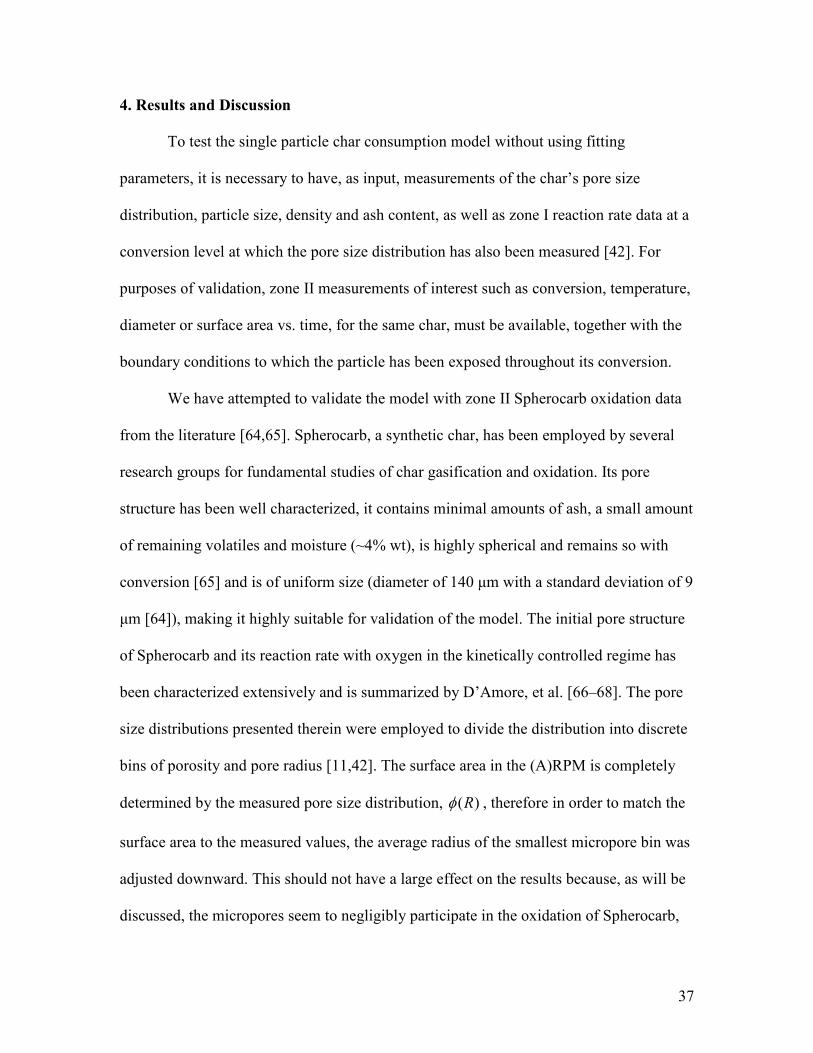
conditions. Table 1 shows the discretized pore structure determined from the data of

D’Amore et al. [66]. The initial surface area for each pore size can be calculated from

( )i iRφ using Eq. (18) and is also shown in Table 1.

Table 1. Parameters employed in pore size distribution of Spherocarb char.

Micropores Mesopores Macropores

Ri (Å) 4.0 10.8 65.1 665.2 5721.8 26078

iφ (m3/m3) 0.1289 0.0204 0.0364 0.0707 0.1001 0.3241

Si (m2/m3) 5.4x108 2.6x107 7.3x106 1.2x106 1.8x105 1.0x105

D’Amore has measured the reaction rates for Spherocarb particles in oxygen at

several different temperatures and oxygen concentrations as a function of conversion [67]

using an electrodynamic balance and a TGA and also summarized measurements taken

by Floess [69] and Hurt using a TGA [70]. Since the pore structure characterization is

done at zero conversion, the reaction rate must be extrapolated back to zero conversion as

well in order to apply the method of the ARPM in determining the intrinsic (per unit area)

rate of oxidation. For this purpose, the method described by Su and Perlmutter [71] was

used to ananlyze the Spherocarb data measured via TGA at temperatures of 673, 703 and

768 K and using only the data points up to 50% conversion for accuracy [71]. Once the

apparent rate is determined, the intrinsic pre-exponential factor is estimated by

normalizing by the participating surface area, since the activation energy and the order of

39

reaction have also been experimentally determined [67]. The intrinsic rate of oxidation

determined by the ARPM and Su and Perlmutter’s method is shown in Table 2. A more

detailed discussion of the calculation of the pre-exponential factor is given elsewhere

[72], but briefly, the value was calculated by averaging the measurements at 703 and 768

K since those measurements of reactivity with conversion closely fit the evolution

predicted by the (A)RPM. The reaction order and activation energy were also taken from

[67].

Using the method of the ARPM to estimate the surface area participating in the

oxidation reaction [42] and the configurational diffusion parameter for oxygen in char

given by Salatino and Zimbardi [73], it has been calculated that the micropores contribute

negligibly to the oxidation of Spherocarb, even in what is ostensibly the kinetically

controlled regime. This is in agreement with the evidence of D’Amore et al. [66] who

found that the normalized micropore size distribution of Spherocarb was remarkably

constant with conversion during oxidation experiments and with the results of D’Amore

et al. [68] based on the reaction rate variation with conversion. However, it is opposite

the conclusion of Hurt et al. [74], which was based on the absence of a particle-size

effect, SEM observation that macropores did not exhibit growth with conversion and a

pore-scale Thiele analysis.

40

Table 2. Intrinsic kinetic parameters for Spherocarb combustion and gasification.

Reaction A [mol /m2 s atmn] E [kJ/mol] n

C+O2 29,180 150.6 1.0

C+H2O 55,248 281.2 0.4

C+CO2 18,416 281.2 0.4

Although it hasn’t been considered in some previous modeling of Waters’

experiments [64,65], char gasification reactions may be significant since the gas mixture

is 16-20% H2O and 2-3% CO2 by volume and particle temperatures typically peak

between 1700 and 2100 K; conditions under which gasification might be expected to play

a non-negligible role. Furthermore, although the intrinsic reaction rate of carbon with

steam is much slower than the reaction with oxygen [75], steam is known to be able to

penetrate and react in small pores that are often inaccessible to oxygen [76] and

Spherocarb particles have a high level of microporosity compared to typical char

particles.

For this validation study, which simulates combustion at atmospheric pressure, nth

order heterogeneous reaction rate forms have been employed. For carbon oxidation, nth

order behavior has been explained as being a consequence of the distribution of

activation energies for combustion among the carbon sites [45]. Although gasification

reactions (R1) and (R3) are most realistically modeled using a Langmuir-Hinshelwood

rate form [77], especially at high pressures [78], for the low and limited partial pressure

41

ranges encountered throughout the char conversion in these experiments, a power law

rate form was deemed acceptable and employed for its simplifying effects and due to the

lack of experimental data available for the rate constants contained in a Langmuir-

Hinshelwood expression [79].

Steam gasification data for uncatalyzed Spherocarb does not exist in the literature.

However, Floess has performed kinetic measurements on the reaction rate parameters of

Spherocarb char with carbon dioxide [69] and this can be used to estimate the steam

gasification rate as well. Walker et al. [80] has suggested that the apparent reaction rate

of char with steam is roughly three times that of the rate with carbon dioxide, while

Harris and Smith have also found a similar ratio to hold for different chars in their

measurements [75]. Shaddix et al. have summarized data from several researchers and

concluded that for a given char, the reaction rate with steam is indeed roughly three times

its rate with CO2 [79]. Furthermore, the experimental data in the literature as well as

theoretical considerations indicate the activation energy for the C+H2O reaction is very

close to that of the C+CO2 reaction, meaning that the pre-exponential factor of the former

is simply three times that of the latter [79].

The same procedure used to determine the intrinsic kinetics of Spherocarb

oxidation was followed for the C+CO2 kinetics using the data of Floess [69] at four

temperatures ranging from 1240-1350 K. The activation energy was determined by

Floess et al. [81] and although the order of reaction was not measured, based on the order

determined for several chars in the literature [61], a value of n=0.4 was assigned. The

intrinsic reaction rate parameters for steam and carbon dioxide are shown in Table 5.2.

The homogeneous reaction of carbon monoxide with oxygen in the boundary layer

42

surrounding Spherocarb particles is deemed to be important by Waters et al. [64] and

Tognotti et al. [46], especially in the presence of water vapor. Therefore reactions (R4)

and (R5) for the oxidation of carbon monoxide and hydrogen were also included in the

simulation.

It was not necessary to include a submodel for the ash behavior in this case, since

Spherocarb has minimal ash content [68]. However, it was necessary to decide whether to

allow for the peripheral fragmentation in the simulation. Spherocarb, like some other

highly microporous chars, has been known to undergo shrinkage in the kinetic regime,

which is thought to be caused by atomic rearrangements (densification) rather than

peripheral fragmentation [82]. Although it is not negligible, the shrinkage is less

significant earlier in its conversion. Since Waters’ data is taken in regime II, in which the

mechanism of shrinkage is unknown and because the extent of shrinkage is smaller at the

lower conversion levels measured and there is not a model consistent with the (A)RPM

that can account for shrinkage, in what follows the measured (r/r0) vs. X data have simply

been used to form the ODE for particle radius, without allowing for any conversion to be

caused by the shrinkage, so that the mass balance is satisfied. In other words, the only

effect shrinkage has in the simulations is to reduce the particle’s diameter; no structural

rearrangements (e.g. densification, pore elimination) are incorporated and no conversion

due to diameter reduction is counted toward the overall conversion. If, as hypothesized

[66], micropore elimination is the mechanism by which shrinkage occurs for this char,

this approach seems an appropriate way to calculate conversion, since micropores do not

participate in the char oxidation. This implies, however, that the gasification rates may be

somewhat over-estimated in what follows, since char gasification occurs on the

43

micropores to a large extent and the micropore surface area could, in reality, decrease

relative to the values calculated, due to shrinkage.

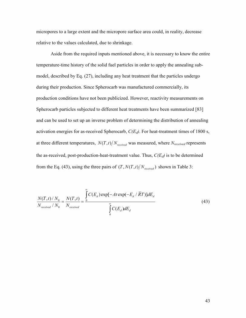
Aside from the required inputs mentioned above, it is necessary to know the entire

temperature-time history of the solid fuel particles in order to apply the annealing sub-

model, described by Eq. (27), including any heat treatment that the particles undergo

during their production. Since Spherocarb was manufactured commercially, its

production conditions have not been publicized. However, reactivity measurements on

Spherocarb particles subjected to different heat treatments have been summarized [83]

and can be used to set up an inverse problem of determining the distribution of annealing

activation energies for as-received Spherocarb, C(Ed). For heat-treatment times of 1800 s,

at three different temperatures, ( , ) receivedN T t N was measured, where Nreceived represents

the as-received, post-production-heat-treatment value. Thus, C(Ed) is to be determined

from the Eq. (43), using the three pairs of ( , ( , ) )receivedT N T t N shown in Table 3:

0 0

0

0

( ) exp[ exp( / )]( , ) / ( , )

/( )

d d d

received received

d d

C E At E RT dEN T t N N T t

N N NC E dE

∞

∞

− −

= =∫

∫ (43)

44

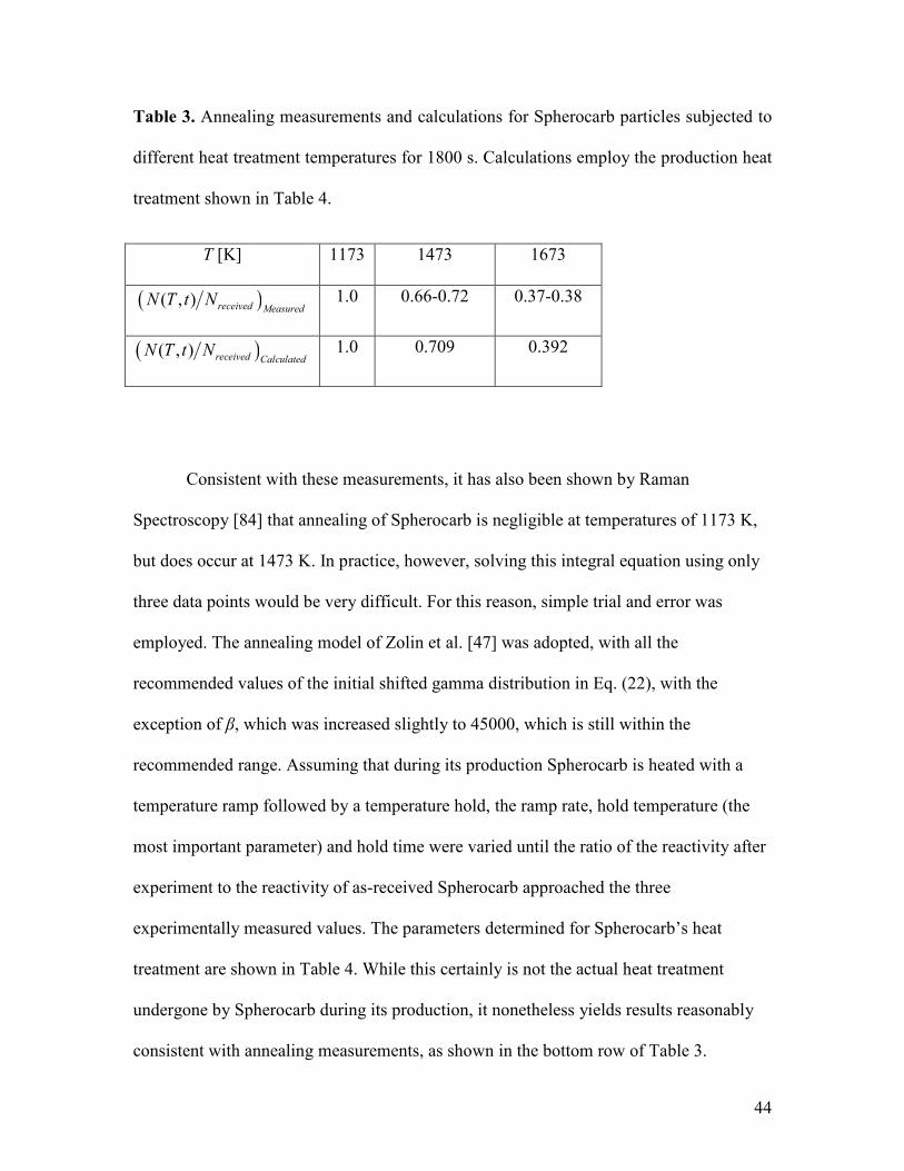
Table 3. Annealing measurements and calculations for Spherocarb particles subjected to

different heat treatment temperatures for 1800 s. Calculations employ the production heat

treatment shown in Table 4.

T [K] 1173 1473 1673

( )( , ) received MeasuredN T t N 1.0 0.66-0.72 0.37-0.38

( )( , ) received CalculatedN T t N 1.0 0.709 0.392

Consistent with these measurements, it has also been shown by Raman

Spectroscopy [84] that annealing of Spherocarb is negligible at temperatures of 1173 K,

but does occur at 1473 K. In practice, however, solving this integral equation using only

three data points would be very difficult. For this reason, simple trial and error was

employed. The annealing model of Zolin et al. [47] was adopted, with all the

recommended values of the initial shifted gamma distribution in Eq. (22), with the

exception of β, which was increased slightly to 45000, which is still within the

recommended range. Assuming that during its production Spherocarb is heated with a

temperature ramp followed by a temperature hold, the ramp rate, hold temperature (the

most important parameter) and hold time were varied until the ratio of the reactivity after

experiment to the reactivity of as-received Spherocarb approached the three

experimentally measured values. The parameters determined for Spherocarb’s heat

treatment are shown in Table 4. While this certainly is not the actual heat treatment

undergone by Spherocarb during its production, it nonetheless yields results reasonably

consistent with annealing measurements, as shown in the bottom row of Table 3.

45

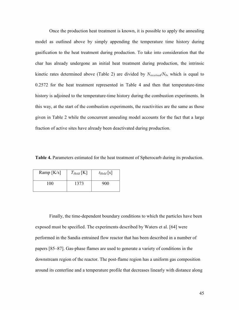
Once the production heat treatment is known, it is possible to apply the annealing

model as outlined above by simply appending the temperature time history during

gasification to the heat treatment during production. To take into consideration that the

char has already undergone an initial heat treatment during production, the intrinsic

kinetic rates determined above (Table 2) are divided by Nreceived/N0, which is equal to

0.2572 for the heat treatment represented in Table 4 and then that temperature-time

history is adjoined to the temperature-time history during the combustion experiments. In

this way, at the start of the combustion experiments, the reactivities are the same as those

given in Table 2 while the concurrent annealing model accounts for the fact that a large

fraction of active sites have already been deactivated during production.

Table 4. Parameters estimated for the heat treatment of Spherocarb during its production.

Ramp [K/s] THold [K] tHold [s]

100 1373 900

Finally, the time-dependent boundary conditions to which the particles have been

exposed must be specified. The experiments described by Waters et al. [64] were

performed in the Sandia entrained flow reactor that has been described in a number of

papers [85–87]. Gas-phase flames are used to generate a variety of conditions in the

downstream region of the reactor. The post-flame region has a uniform gas composition

around its centerline and a temperature profile that decreases linearly with distance along

46

the axis at a rate of roughly -1 K/mm [85]. Based on Fig. 2 in the study by Murphy and

Shaddix [87], the location of the peak temperature was estimated. The gas temperature in

the region before the peak temperature is estimated by comparison with Fig. 2 in Molina

and Shaddix [88] and with Fig. 1 in the study of Shaddix and Molina [89]. The particle

velocity is roughly 2.5 m/s [64], enabling conversion of position in the reactor to

residence time. The gas flow relative to the particle has typically been neglected in

modeling this reactor since the Reynolds number based on this slip velocity is ~10-6 [87],

permitting the use of a spherically symmetric domain with only a radial velocity

component. The wall temperature, used in calculating radiation from the particle, is taken

as 500 K for this reactor [64,86,87] and the particle emissivity is given as 0.85 [64].

Measurements of char conversion and particle temperature were performed at three

heights in the reactor (12.7, 19.1 and 25.4 cm) and have been described elsewhere [64].

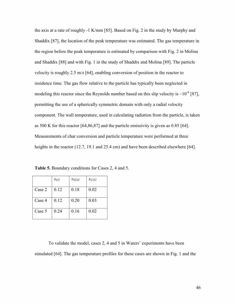
Table 5. Boundary conditions for Cases 2, 4 and 5.

xO2 xH2O xCO2

Case 2 0.12 0.18 0.02

Case 4 0.12 0.20 0.03

Case 5 0.24 0.16 0.02

To validate the model, cases 2, 4 and 5 in Waters’ experiments have been

simulated [64]. The gas temperature profiles for these cases are shown in Fig. 1 and the

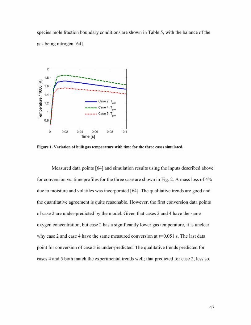
47

species mole fraction boundary conditions are shown in Table 5, with the balance of the

gas being nitrogen [64].

0 0.02 0.04 0.06 0.08 0.1

0.8

1

1.2

1.4

1.6

1.8

2

Time [s]

Te

mp

era

ture

/ 1

00

0 [

K]

Case 2, Tgas

Case 4, Tgas

Case 5, Tgas

Figure 1. Variation of bulk gas temperature with time for the three cases simulated.

Measured data points [64] and simulation results using the inputs described above

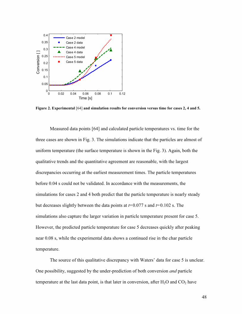
for conversion vs. time profiles for the three case are shown in Fig. 2. A mass loss of 4%

due to moisture and volatiles was incorporated [64]. The qualitative trends are good and

the quantitative agreement is quite reasonable. However, the first conversion data points

of case 2 are under-predicted by the model. Given that cases 2 and 4 have the same

oxygen concentration, but case 2 has a significantly lower gas temperature, it is unclear

why case 2 and case 4 have the same measured conversion at t=0.051 s. The last data

point for conversion of case 5 is under-predicted. The qualitative trends predicted for

cases 4 and 5 both match the experimental trends well; that predicted for case 2, less so.

48

0 0.02 0.04 0.06 0.08 0.1 0.120

0.05

0.1

0.15

0.2

0.25

0.3

0.35

0.4

Time [s]

Co

nv

ers

ion

[ ]

Case 2 model

Case 2 data

Case 4 model

Case 4 data

Case 5 model

Case 5 data

Figure 2. Experimental [64] and simulation results for conversion versus time for cases 2, 4 and 5.

Measured data points [64] and calculated particle temperatures vs. time for the

three cases are shown in Fig. 3. The simulations indicate that the particles are almost of

uniform temperature (the surface temperature is shown in the Fig. 3). Again, both the

qualitative trends and the quantitative agreement are reasonable, with the largest

discrepancies occurring at the earliest measurement times. The particle temperatures

before 0.04 s could not be validated. In accordance with the measurements, the

simulations for cases 2 and 4 both predict that the particle temperature is nearly steady

but decreases slightly between the data points at t=0.077 s and t=0.102 s. The

simulations also capture the larger variation in particle temperature present for case 5.

However, the predicted particle temperature for case 5 decreases quickly after peaking

near 0.08 s, while the experimental data shows a continued rise in the char particle

temperature.

The source of this qualitative discrepancy with Waters’ data for case 5 is unclear.

One possibility, suggested by the under-prediction of both conversion and particle

temperature at the last data point, is that later in conversion, after H2O and CO2 have

49

reacted on the surface of the micropores increasing their width and after oxidation of

mesopores has decreased the length of micropores, oxygen begins to react to a greater

extent on micropores than predicted by the model. A possible contribution to the under-

prediction of particle temperature could be shrinkage (densification), which is thought to

be caused by the elimination of microporosity, as discussed above, and which decreases

the surface area available for the endothermic gasification reactions.

Taken together, Figs. 2 and 3 provide a reasonable level of confidence in the

overall model and in its ability to predict the behavior of well-characterized char particles

subject to conditions in which multiple reactions occur in the regime of intra-particle

diffusion limitations. This has been done without using fitting parameters, although the

parameters representing the pore size at which configurational diffusion becomes

significant (see Eq. (A.5)), σ , are not well-known for CO2 and H2O and can influence

the simulation results because Spherocarb particles have a large microporous surface

area. Nonetheless, the configurational diffusion parameters have been fixed based on

literature observations and a more extensive discussion, as well as a parameter study, is

given elsewhere [72]. For these simulations, 2

20O nmσ = , 2

5CO nmσ = and

21H O nmσ = .

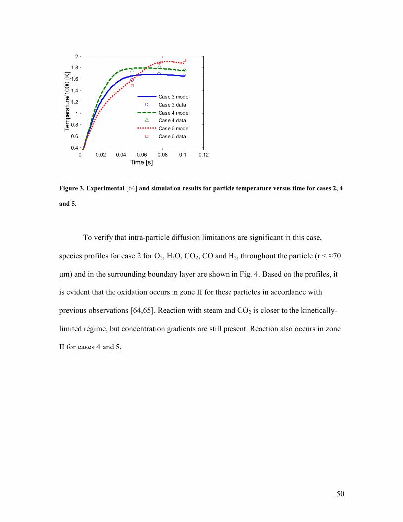
50

0 0.02 0.04 0.06 0.08 0.1 0.12

0.4

0.6

0.8

1

1.2

1.4

1.6

1.8

2

Time [s]

Te

mp

era

ture

/10

00

[K

]

Case 2 model

Case 2 data

Case 4 model

Case 4 data

Case 5 model

Case 5 data

Figure 3. Experimental [64] and simulation results for particle temperature versus time for cases 2, 4

and 5.

To verify that intra-particle diffusion limitations are significant in this case,

species profiles for case 2 for O2, H2O, CO2, CO and H2, throughout the particle (r < ≈70

µm) and in the surrounding boundary layer are shown in Fig. 4. Based on the profiles, it

is evident that the oxidation occurs in zone II for these particles in accordance with

previous observations [64,65]. Reaction with steam and CO2 is closer to the kinetically-

limited regime, but concentration gradients are still present. Reaction also occurs in zone

II for cases 4 and 5.

51

0 100 200 300 400 5000

0.02

0.04

0.06

0.08

0.1

0.12

0.14

0.16

0.18

0.2

Position [µm]

Mo

le F

rac

tio

n [

]

O2

H2O

CO2

CO

H2

Figure 4. Profiles of species mole fractions for case 2 at t=0.077 s.

The impact of the pore structure evolution and of the gasification reaction during

these combustion simulations are illustrated in Fig. 5, which shows conversion and

particle temperature for case 2, using both the ARPM and the RPM, with and without

accounting for the gasification reactions. In applying the RPM, all pore-scale

effectiveness factors are set to unity and the reaction rate parameters are normalized

accordingly. In other words, the intrinsic char oxidation rate is much lower when using

the RPM, since the surface area on which it occurs is taken to be much larger. In this

way, the initial apparent reactivity is identical for the RPM and ARPM, although the pore

structure will evolve differently in the two cases.

Figures 5(a) and 5(b) show that, in the case of the ARPM, neglecting the

gasification reactions decreases conversion at t=0.102 s from 0.22 to 0.205 and increases

particle temperature by a maximum of 40 K. For the RPM, these disparities are somewhat

greater (0.255 to 0.225 and ~65 K). When using the RPM, the conversion is higher for

both cases (gasification on and off), respectively, than when using the ARPM. This is

52

because the RPM allows all pore sizes to participate in all reactions fully and therefore

the micropore growth (qmicro) is the same as the growth of all other pores (instead of

experiencing mostly overlap), thus slowing the decrease in surface area with conversion

experienced by the particle.

0 0.02 0.04 0.06 0.08 0.1 0.120

0.05

0.1

0.15

0.2

0.25

0.3

0.35

Time [s]

Co

nv

ers

ion

[ ]

Case 2, ARPM, Gasif. ON

Case 2, RPM, Gasif. ON

Case 2, ARPM, Gasif. OFF

Case 2, RPM, Gasif. OFF

0 0.02 0.04 0.06 0.08 0.1 0.12

0.4

0.6

0.8

1

1.2

1.4

1.6

1.8

Time [s]

Te

mp

era

ture

/10

00

[K

]

Case 2, ARPM, Gasif ication ON

Case 2, RPM, Gasif ication ON

Case 2, ARPM, Gasif ication OFF

Case 2, RPM, Gasif ication OFF

Figure 5. Simulation results and Waters’ data for case 2, using the ARPM and the RPM, with and

without accounting for the gasification reactions: (a) conversion vs. time, and (b) particle

temperature vs. time.

Figure 6(a) shows the evolution of the total, normalized particle surface with

conversion, corresponding to the cases of Fig. 5. Again, due to the RPM’s assumption

that all pore sizes at a give location grow by the same amount, q, the char surface area

shows a peak with conversion because the micropores are no longer subject mostly to

overlap by larger pores, as they are in the case of the ARPM, in which oxidation occurs

on the meso- and macro-pores. Since the micropore surface area is the dominant portion

of the total area, the surface area is larger when using the RPM than the ARPM. When

gasification reactions are turned on, the surface area is larger in both cases: in the case of

53

the RPM (in which all pore-scale effectiveness factors are unity anyway) the surface area

is slightly larger because gasification reactions change the conversion profile within the

particle, which affects Tot TotdS dX , even though the local dS dX is identical

everywhere. For the ARPM, the difference is more significant, due to the fact that in

contrast to oxidation, which occurs almost mostly on the mesopores (since micropores

participate minimally in oxidation and the macropore surface area is relatively small),

gasification reactions occur on the micropores to a degree, increasing the surface area

compared to the case of pure oxidation.

0 0.05 0.1 0.15 0.20.8

0.85

0.9

0.95

1

Total Conversion [ ]

No

rma

lize

d S

urf

ac

e A

rea

[m

2/m

3]

ARPM, Gasif. ON

RPM, Gasif . ON

ARPM, Gasif. OFF

RPM, Gasif . OFF

0 10 20 30 40 50 60 700

0.1

0.2

0.3

0.4

Position [µm]

Co

nv

ers

ion

[ ]

Micropores, Gasif. ON

Mesopores, Gasif. ON

Macropores, Gasif. ON

Micropores, Gasif. OFF

Mesopores, Gasif. OFF

Macropores, Gasif. OFF

Figure 6. (a) Variation of total surface area with total char conversion, for case 2, using both the

ARPM and the RPM, with and without accounting for gasification, (b) profiles of conversion due to

reaction on each pore size, for the ARPM only, with gasification reactions turned on and off.

Figure 6b uses Eq. (20) to calculate the final profiles of conversion that result

from reaction on each pore class using the ARPM, with gasification reactions both

considered and neglected, at t=0.102 s for case 2. Whether or not gasification reactions

are assumed to occur, most of the conversion occurs on the mesopores, since char

54

oxidation is the dominant reaction and oxidation on the micropores is minimal. When

gasification reactions are considered, it is indeed seen that micropores are able to

participate in char reactions and contribute to conversion, to an extent, due to the ability

of H2O to react on micropores (in contrast to O2). Furthermore, the overall conversion

profile within the particle is more uniform when gasification reactions are considered

because H2O and CO2 experience fewer diffusion limitations than O2. When gasification

reactions are neglected, micropore conversion is negligible and reaction on the mesopores

accounts for the vast majority of conversion.

Table 6. Discretized pore size distribution for “char B”.

Ri (Å) 7.1 40 90 1877

iφ 0.1089 0.016 0.015 0.1483

When using the Feng and Stewart model, the flux in the micropores may not

satisfy the smooth field hypothesis in the presence of fast reactions (e.g oxidation), as

mentioned in Section 2, and the correction of Jackson is not applicable in this case [20].

As also mentioned by Jackson, the contribution of the micropore flux is typically small

compared to transport in other pore sizes. A comparison of simulations of case 2

employing with and without accounting for the micropore contribution to the fluxes was

performed. The difference in the overall conversion results is negligible; they are

identical to the third decimal place.

The Feng and Stewart model explicitly accounts for multi-modal pore structures,

while the Dusty Gas model uses an average pore size in its calculation of parameters

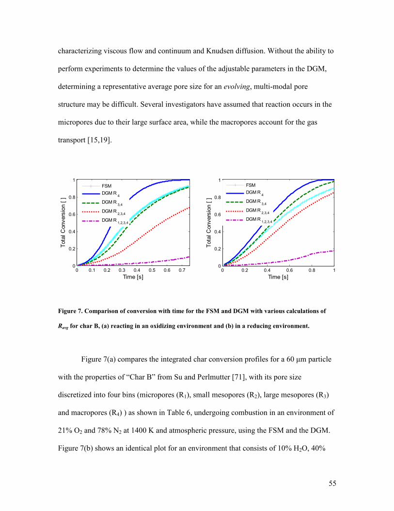
55

characterizing viscous flow and continuum and Knudsen diffusion. Without the ability to

perform experiments to determine the values of the adjustable parameters in the DGM,

determining a representative average pore size for an evolving, multi-modal pore

structure may be difficult. Several investigators have assumed that reaction occurs in the

micropores due to their large surface area, while the macropores account for the gas

transport [15,19].

0 0.1 0.2 0.3 0.4 0.5 0.6 0.70

0.2

0.4

0.6

0.8

1

Time [s]

To

tal

Co

nv

ers

ion

[ ]

FSM

DGM R4

DGM R3,4

DGM R2,3,4

DGM R1,2,3,4

0 0.2 0.4 0.6 0.8 1

0

0.2

0.4

0.6

0.8

1

Time [s]

To

tal

Co

nv

ers

ion

[ ]

FSM

DGM R4

DGM R3,4

DGM R2,3,4

DGM R1,2,3,4

Figure 7. Comparison of conversion with time for the FSM and DGM with various calculations of

Ravg for char B, (a) reacting in an oxidizing environment and (b) in a reducing environment.

Figure 7(a) compares the integrated char conversion profiles for a 60 µm particle

with the properties of “Char B” from Su and Perlmutter [71], with its pore size

discretized into four bins (micropores (R1), small mesopores (R2), large mesopores (R3)

and macropores (R4) ) as shown in Table 6, undergoing combustion in an environment of

21% O2 and 78% N2 at 1400 K and atmospheric pressure, using the FSM and the DGM.

Figure 7(b) shows an identical plot for an environment that consists of 10% H2O, 40%

56

CO2 and 50% N2 at 1900 K and atmospheric pressure. The tortuosity required by the

DGM is set to three, in accordance with the FSM value of 1/3 applicable for the ARPM

geometry. All other model parameters are identical, and the ARPM has been applied in

both cases. The average pore radius in the DGM has been obtained by taking the

hydraulic radius, 2hr Sφ= , where the porosity and surface area include contributions

from different pore sizes, as indicated in the legend of the figure.

For Fig. 7(a) it is observed that inclusion of the micropores in the calculation of rh

produces results that differ significantly from the predictions of the FSM, while

calculation of rh by including all macropores and large mesopores produces a result

similar to the FSM predictions. The results in Fig 7(b) are slightly different in that the

FSM is closest to the DGM with ravg based on the two largest pore sizes, but later in

conversion, the results from the FSM begin to approach that of the DGM with ravg based

on the three largest pore sizes. In fact, both figures indicate that the FSM yields a

conversion that increases less rapidly than the DGM later in conversion. Figure 7 was

obtained for a situation in which intra-particle diffusion limitations were deemed

significant throughout the course of conversion, based on the profiles of the reactants and

products throughout the porous structure (not shown).

For these combustion and gasification conditions, the practice of using the DGM

for calculation of the fluxes by excluding the micropores and possibly smaller mesopores

yields results similar to the slightly more complex Feng and Stewart model, which

considers each pore size separately. The reason for the distortion of the results of the

DGM by including the micropores is due to their large contribution to the surface area,

which drastically reduces the average pore radius parameter, whereas neglecting the

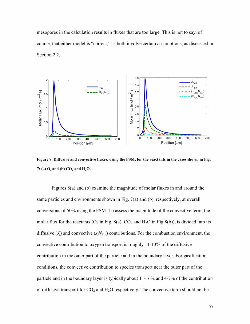
57

mesopores in the calculation results in fluxes that are too large. This is not to say, of

course, that either model is “correct,” as both involve certain assumptions, as discussed in

Section 2.2.

0 100 200 300 400 500 600 7000

0.5

1

1.5

2

Position [µm]

Mo

lar

Flu

x [

mo

l /

m2

s]

JO2

(xO2

NTot

)

0 100 200 300 400 500 600 7000

0.2

0.4

0.6

0.8

1

1.2

1.4

1.6

Position [µm]

Mo

lar

Flu

x [

mo

l /

m2

s]

J

CO2

JH2O

(xCO2

NTot

)

(xH2O

NTot

)

Figure 8. Diffusive and convective fluxes, using the FSM, for the reactants in the cases shown in Fig.

7: (a) O2 and (b) CO2 and H2O.

Figures 8(a) and (b) examine the magnitude of molar fluxes in and around the

same particles and environments shown in Fig. 7(a) and (b), respectively, at overall

conversions of 50% using the FSM. To assess the magnitude of the convective term, the

molar flux for the reactants (O2 in Fig. 8(a), CO2 and H2O in Fig 8(b)), is divided into its

diffusive (Jj) and convective (xjNTot) contributions. For the combustion environment, the

convective contribution to oxygen transport is roughly 11-13% of the diffusive

contribution in the outer part of the particle and in the boundary layer. For gasification

conditions, the convective contribution to species transport near the outer part of the

particle and in the boundary layer is typically about 11-16% and 4-7% of the contribution

of diffusive transport for CO2 and H2O respectively. The convective term should not be

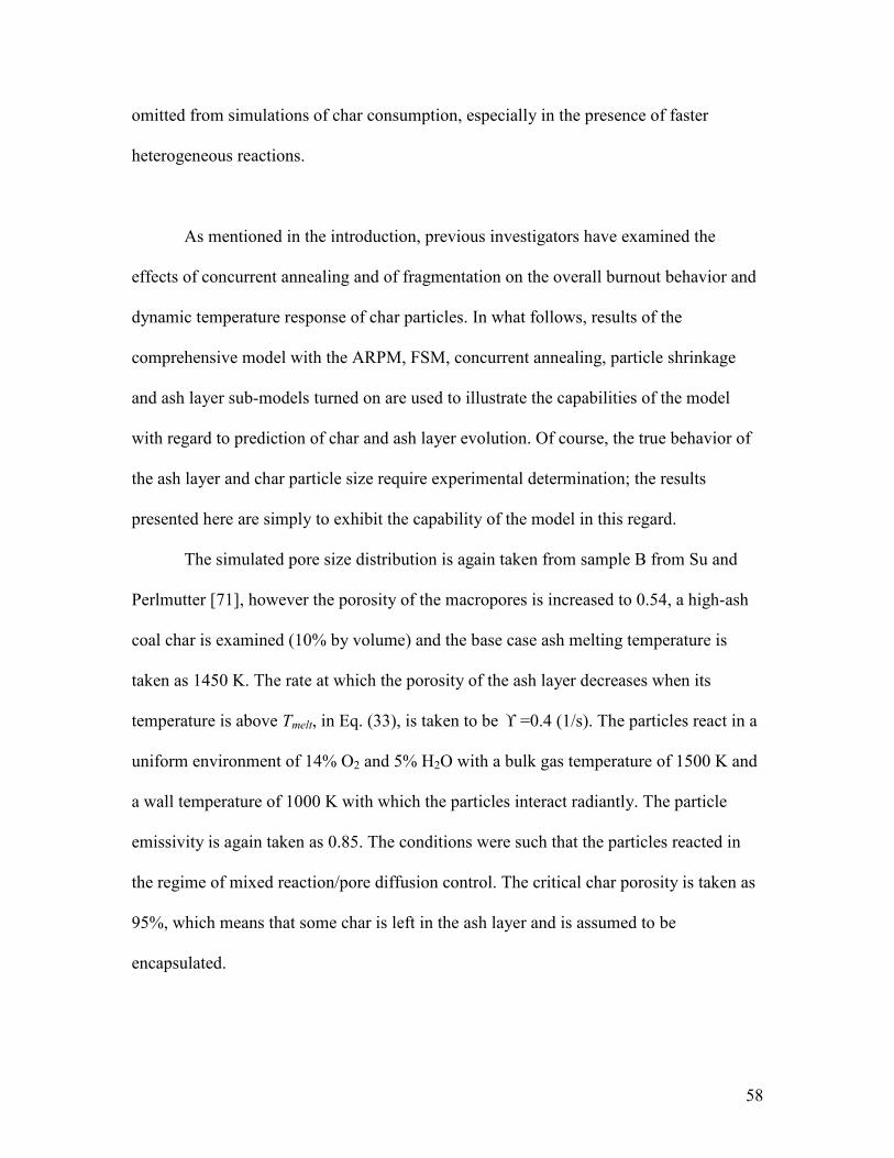
58

omitted from simulations of char consumption, especially in the presence of faster

heterogeneous reactions.

As mentioned in the introduction, previous investigators have examined the

effects of concurrent annealing and of fragmentation on the overall burnout behavior and

dynamic temperature response of char particles. In what follows, results of the

comprehensive model with the ARPM, FSM, concurrent annealing, particle shrinkage

and ash layer sub-models turned on are used to illustrate the capabilities of the model

with regard to prediction of char and ash layer evolution. Of course, the true behavior of

the ash layer and char particle size require experimental determination; the results

presented here are simply to exhibit the capability of the model in this regard.

The simulated pore size distribution is again taken from sample B from Su and

Perlmutter [71], however the porosity of the macropores is increased to 0.54, a high-ash

coal char is examined (10% by volume) and the base case ash melting temperature is

taken as 1450 K. The rate at which the porosity of the ash layer decreases when its

temperature is above Tmelt, in Eq. (33), is taken to be ϒ =0.4 (1/s). The particles react in a

uniform environment of 14% O2 and 5% H2O with a bulk gas temperature of 1500 K and

a wall temperature of 1000 K with which the particles interact radiantly. The particle

emissivity is again taken as 0.85. The conditions were such that the particles reacted in

the regime of mixed reaction/pore diffusion control. The critical char porosity is taken as

95%, which means that some char is left in the ash layer and is assumed to be

encapsulated.

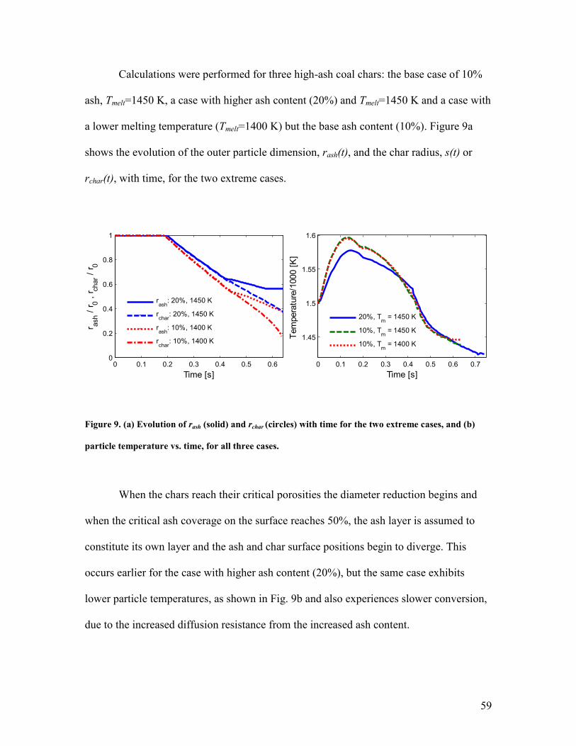
59

Calculations were performed for three high-ash coal chars: the base case of 10%

ash, Tmelt=1450 K, a case with higher ash content (20%) and Tmelt=1450 K and a case with

a lower melting temperature (Tmelt=1400 K) but the base ash content (10%). Figure 9a

shows the evolution of the outer particle dimension, rash(t), and the char radius, s(t) or

rchar(t), with time, for the two extreme cases.

0 0.1 0.2 0.3 0.4 0.5 0.60

0.2

0.4

0.6

0.8

1

Time [s]

r as

h /

r0 ,

rc

ha

r / r

0

rash

: 20%, 1450 K

rchar

: 20%, 1450 K

rash

: 10%, 1400 K

rchar

: 10%, 1400 K

0 0.1 0.2 0.3 0.4 0.5 0.6 0.7

1.45

1.5

1.55

1.6

Time [s]

Te

mp

era

ture

/10

00

[K

]

20%, Tm

= 1450 K

10%, Tm

= 1450 K

10%, Tm

= 1400 K

Figure 9. (a) Evolution of rash (solid) and rchar (circles) with time for the two extreme cases, and (b)

particle temperature vs. time, for all three cases.

When the chars reach their critical porosities the diameter reduction begins and

when the critical ash coverage on the surface reaches 50%, the ash layer is assumed to

constitute its own layer and the ash and char surface positions begin to diverge. This

occurs earlier for the case with higher ash content (20%), but the same case exhibits

lower particle temperatures, as shown in Fig. 9b and also experiences slower conversion,

due to the increased diffusion resistance from the increased ash content.

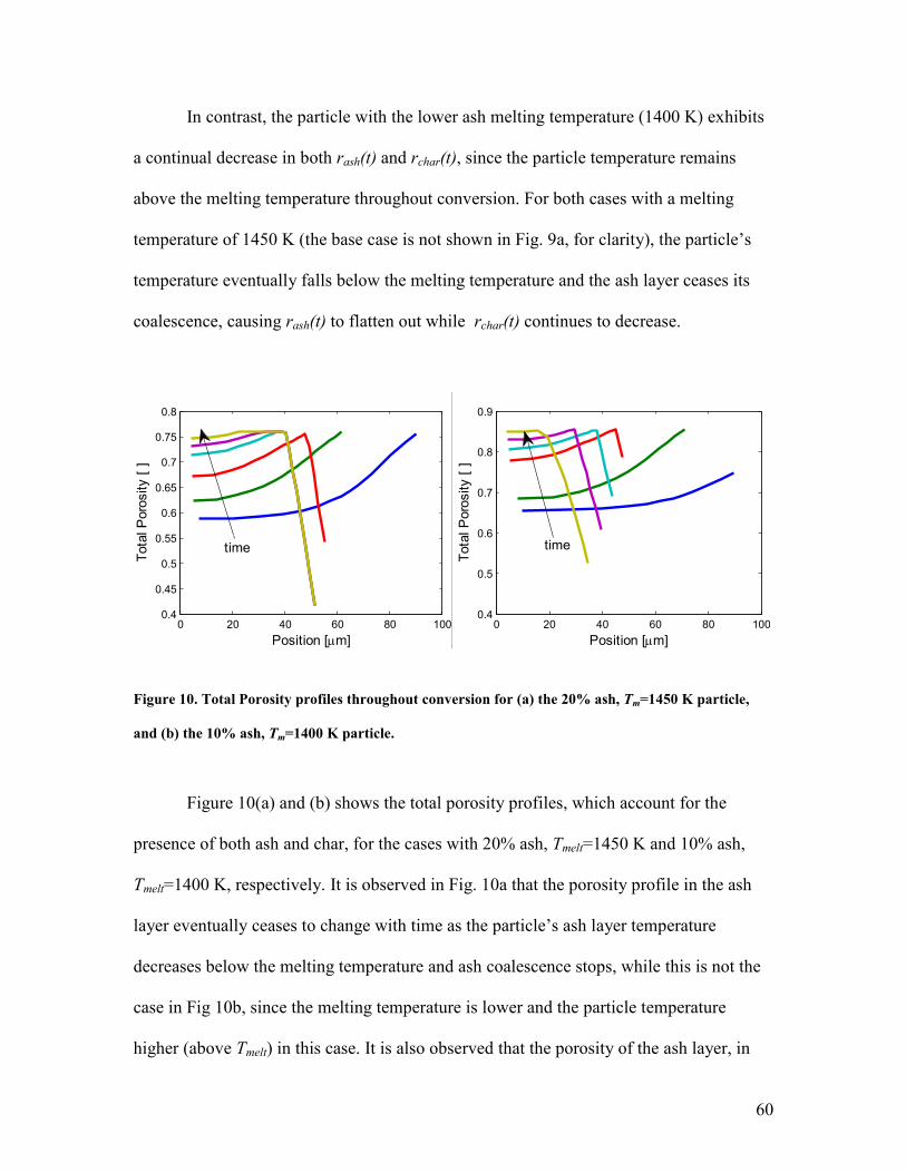
60

In contrast, the particle with the lower ash melting temperature (1400 K) exhibits

a continual decrease in both rash(t) and rchar(t), since the particle temperature remains

above the melting temperature throughout conversion. For both cases with a melting

temperature of 1450 K (the base case is not shown in Fig. 9a, for clarity), the particle’s

temperature eventually falls below the melting temperature and the ash layer ceases its

coalescence, causing rash(t) to flatten out while rchar(t) continues to decrease.

0 20 40 60 80 1000.4

0.45

0.5

0.55

0.6

0.65

0.7

0.75

0.8

Position [µm]

To

tal

Po

ros

ity

[ ]

time

0 20 40 60 80 1000.4

0.5

0.6

0.7

0.8

0.9

Position [µm]

To

tal

Po

ros

ity

[ ]

time

Figure 10. Total Porosity profiles throughout conversion for (a) the 20% ash, Tm=1450 K particle,

and (b) the 10% ash, Tm=1400 K particle.

Figure 10(a) and (b) shows the total porosity profiles, which account for the

presence of both ash and char, for the cases with 20% ash, Tmelt=1450 K and 10% ash,

Tmelt=1400 K, respectively. It is observed in Fig. 10a that the porosity profile in the ash

layer eventually ceases to change with time as the particle’s ash layer temperature

decreases below the melting temperature and ash coalescence stops, while this is not the

case in Fig 10b, since the melting temperature is lower and the particle temperature

higher (above Tmelt) in this case. It is also observed that the porosity of the ash layer, in

61

Fig 10a, decreases below the values observed in Fig 10b, because the ash layer has had a

longer time to undergo coalescence since the higher ash content leads to a faster buildup

of ash on the surface.

5. Conclusions

A comprehensive, predictive model for the gasification and combustion of multi-

modal, porous char particles has been developed. The model is a one–dimensional,

spherically symmetric, transient simulation of a reacting, porous char particle and its

surrounding boundary layer. The model incorporates the adaptive random pore model

(ARPM), which is consistent with an evolving, multi-modal porous structure and which

extends the original random pore model to allow different pore sizes to grow at different

rates depending on the instantaneous interplay of transport and kinetics at the pore scale,

at different positions within a char particle. Gas transport within the porous structure is

modeled using the flux relations of Feng and Stewart, which are also consistent with a

multi-modal pore structure. The model can account for concurrent annealing, particle size

reduction and the possibility of ash adherence on the particle surface, although these

submodels require the specification of several parameters. The model has been validated

against zone II combustion data for Spherocarb char [64] without the use of fitting

parameters and good agreement with experimental measurements of particle temperature

and conversion have been obtained. The participation of various pore sizes in reaction

and the occurrence of gasification reaction for these particular combustion conditions are

shown to have non-negligible effects on overall conversion and temperature evolution.

For a case with multiple reactants in the regime of intra-particle diffusion limitations, the

62

DGM has been shown to produce results similar to the FSM when the average pore size

parameter is calculated throughout conversion using a hydraulic radius that neglects

micropores and smaller mesopores. Examples of high-ash char particles reacting in an

environment of 14% O2 and 5% H2O have been used to illustrate the full capabilities of

the model in terms of calculating the evolution and porosity of both char and ash layers

separately.

Acknowledgment

This research is funded by the BP-MIT Conversion Research Program.

Nomenclature and Units

A = pre-exponential factor (mol /m2C s (atm)n) or (g /m2

C s (atm)n)

Ad = pre-exponential factor for annealing (1/s)

B0 = Permeability (m2)

C = concentration (mol/m3)

cp = specific heat (J/mol K)

C(Ed) = post heat-treatment distribution of annealing activation energies (mol/J)

D = diffusion coefficient (m2/s)

E = activation energy (J/mol) or (kJ/mol)

Ed = activation energy for annealing (J/mol)

fash = volume fraction of ash in char (-)

F = distribution of active sites with activation energy (mol/J)

J = diffusive flux (mol/m2 s)

63

J��

= diffusive flux vector for all species (mol/m2 s)

k = thermal conductivity (W/m K)

k, kHT = (post-annealing heat treatment) reaction rate constant (molC /m2C s (atm)n)

l0,i = total length of pores i per unit volume (m/m3)

MW = molecular weight (g/mol)

n = number of pore bins, number of gas species, or reaction order

',i jn = expected number of intersections of pores i and j per unit length of pores i (1/m)

N(t)/N0 = fraction of active sites remaining (-)

Nj = Species flux (mol j/m2 s)

NTot = Convective flux (mol/m2 s)

p = pressure (N/m2) or (atm)

q, qi = pore growth variable (uniform or individual) (m)

qrad = radiative heat flux (W/m2)

r = radial position (m)

rash = position of moving ash boundary (m)

rh = hydraulic radius (m)

R = pore radius (m)

ℜ = heterogeneous reaction rate (mol/m2C s) or homogeneous reaction rate (mol/m3 s)

R = universal gas constant (J/mol K)

Rmix = specific gas constant in Eq. (34) (J/kg K)

s = position of moving char boundary, same as rchar (m)

S = total pore surface area (m2C/m3)

Si = pores i surface area (m2C/m3)

64

t = time (s)

T = temperature (K)

u = radial velocity (m/s)

x = mole fraction (-)

X = solid conversion (-)

XTrue,i = solid conversion due to reaction on pores i (-)

Greek Symbols

α = shape parameter in gamma distribution

β = scale parameter in gamma distribution, or sigmoid function defined in Eq. (40)

δ = shift parameter in gamma distribution (J/mol)

iφ = porosity (m3pore i/m

3)

Totφ = total porosity (m3pore/m

3)

,i kη = effectiveness factor for pore i in reaction k (-)

µ = viscosity (kg/m s)

ν = stoichiometric coefficient (mol/mol)

ρ = density (kg/m3)

Trueρ = true solid density (helium density) (kg/m3)

σ = pore radius at which configurational diffusion becomes significant (m)

ς = dimensionless radial coordinate (-)

ξ = coefficient in determining CO/CO2 ratio from reaction (R2)

ψ = Random Pore model structural parameter (-)

65

∆ = expression for DGM or FSM defined in text

rh∆ = heat of reaction (J/mol)

Φ = Thiele modulus (-)

Γ = gamma function

ϒ = rate of decrease in ash layer porosity (1/s)

Subscripts

0 = at initial time t=0 or initial conversion X=0

ash = property of ash

bin = associated with particular annealing time-temperature bin

bulk = property at the bulk gas conditions

continuum = molecular diffusion coefficient

critical = at the critical conversion or porosity

C = char

eff = effective coefficient accounting for gas and solid phase

Final = at final time, at X=1

gas = property of gas

hold = length of time at a given temperature heat treatment

i = pore size

j = gas species (or pore size)

k = reaction index

Kn = Knudsen diffusion coefficient

melt = Temperature at which ash “melts”

66

received = post-production/as-received (in reference to Spherocarb char particles)

s+/-

= at location just below or beyond porous medium/gas interface

s = gas species

solid = property of solid

t = gas species

Tot = total

True,i = due to reaction on pores i

References

[1] R.E. Mitchell, R.J. Kee, P. Glarborg, M.E. Coltrin, Twenty-Third Symposium (International) on Combustion (1990) 1169-1176.

[2] S.Y. Cho, R.A. Yetter, F.L. Dryer, Journal of Computational Physics 102 (1992) 160-179.

[3] J.C. Lee, R.A. Yetter, F.L. Dryer, Combustion and Flame 101 (1995) 387-398.

[4] S. Goel, C.H. Lee, J.P. Longwell, A.F. Sarofim, Energy and Fuels 10 (1996) 1091-1098.

[5] R. Stauch, U. Maas, International Journal of Heat and Mass Transfer 52 (2009) 4584-4591.

[6] M.Y. Ha, B.R. Choi, Combustion and Flame 97 (1994) 1-16.

[7] V. Raghavan, V. Babu, T. Sundararajan, R. Natarajan, International Journal of Heat and Mass Transfer 48 (2005) 5354-5370.

[8] F.J. Higuera, Combustion and Flame 152 (2008) 230-244.

[9] J. Lee, A.G. Tomboulides, S.A. Orszag, R.A. Yetter, F.L. Dryer, Twenty-Sixth Symposium (International) on Combustion (1996) 3059-3065.

[10] G.R. Gavalas, AIChE Journal 26 (1980) 577-585.

[11] G.R. Gavalas, Combustion Science and Technology 24 (1981) 197-210.

67

[12] C. Feng, W.E. Stewart, Ind. Eng. Chem. Res. 12 (1973) 143-147.

[13] S.K. Bhatia, D.D. Perlmutter, AIChE Journal 26 (1980) 379-386.

[14] S.K. Bhatia, D.D. Perlmutter, AIChE Journal 27 (1981) 247-254.

[15] S.V. Sotirchos, N.R. Amundson, AIChE Journal 30 (1984) 537-549.

[16] S.V. Sotirchos, N.R. Amundson, AIChE Journal 30 (1984) 549-556.

[17] E.A. Mason, A.P. Malinauskas, Gas Transport in Porous Media: The Dusty-Gas Model, Elsevier, 1983.

[18] G. Ballal, C.-hsien Li, R. Glowinski, N.R. Amundson, Computer Methods in Applied Mechanics and Engineering 75 (1989) 467-479.

[19] J.I. Morell, N.R. Amundson, S.K. Park, Chemical Engineering Science 45 (1990) 387-401.

[20] R. Jackson, Transport in Porous Catalysts, Elsevier, New York, 1977.

[21] S. Reyes, K.F. Jensen, Chemical Engineering Science 41 (1986) 345-354.

[22] S. Srinivasachar, M.A. Toqan, J.M. Beer, H.M. Ettouney, Combustion Science and Technology 57 (1988) 55-70.

[23] M.J. Biggs, P.K. Agarwal, Chemical Engineering 52 (1997) 941-952.

[24] F.Y. Wang, S.K. Bhatia, Chemical Engineering Journal 56 (2001) 3683-3697.

[25] A. Zolin, A. Jensen, Combustion and Flame 125 (2001) 1341-1360.

[26] E.M. Suuberg, M. Wojtowicz, J.M. Calo, Carbon 27 (1989) 431-440.

[27] R. Hurt, J.K. Sun, M. Lunden, Combustion and Flame 113 (1998) 181-197.

[28] Y. Cai, K. Zygourakis, Ind. Eng. Chem. Res. 42 (2003) 2746-2755.

[29] R.E. Mitchell, L. Ma, B. Kim, Combustion and Flame 151 (2007) 426-436.

[30] G. Ballal, K. Zygourakis, Ind. Eng. Chem. Res. 26 (1987) 1787-1796.

[31] R.H. Hurt, A.F. Sarofim, J.P. Longwell, Fuel 70 (1991) 1079-1082.

[32] I. Aarna, E.M. Suuberg, Twenty-Seventh Symposium (International) on Combustion 27 (1998) 2933-2939.

68

[33] L.R. Radovic, P.L. Walker, R.G. Jenkins, Fuel 62 (1983) 849-856.

[34] P. Salatino, O. Senneca, S. Masi, Carbon 36 (1998) 443-452.

[35] B. Feng, S.K. Bhatia, Carbon 41 (2003) 507-523.

[36] D.G. Roberts, D.J. Harris, T.F. Wall, Energy & Fuels 17 (2003) 887-895.

[37] R. Sahu, R.C. Flagan, G.R. Gavalas, Combustion and Flame 77 (1989) 337-346.

[38] M. Loewenberg, Y.A. Levendis, Combustion and Flame 84 (1991) 47-65.

[39] M. Sahimi, G.R. Gavalas, T.T. Tsotsis, Chemical Engineering Science 45 (1990) 1443-1502.

[40] S.V. Sotirchos, V.N. Burganos, AIChE Journal 34 (1988) 1106-1118.

[41] S.V. Sotirchos, AIChE Journal 35 (1989) 1953-1961.

[42] S.L. Singer, A.F. Ghoniem, Energy and Fuels 25 (2011) 1423-1437.

[43] J.B. Howard, G.C. Williams, D.H. Fine, Symposium (International) on Combustion 14 (1973) 975-986.

[44] A.K. Varma, A.U. Chatwani, F.V. Bracco, Combustion and Flame 64 (1986) 233-236.

[45] R.H. Hurt, B.S. Haynes, Proceedings of the Combustion Institute 30 (2005) 2161-2168.

[46] L. Tognotti, J.P. Longwell, A.F. Sarofim, Symposium (International) on Combustion 23 (1990) 1207-1213.

[47] A. Zolin, A. Jensen, K. Dam-Johansen, Proceedings of the Combustion Institute 28 (2000) 2181-2188.

[48] A.R. Kerstein, S. Niksa, Proceedings of the Combustion Institute 20 (1984) 941-949.

[49] G. Liu, H. Wu, R.P. Gupta, J.A. Lucas, A.G. Tate, T.F. Wall, Fuel 79 (2000) 627-633.

[50] B. Feng, S.K. Bhatia, Energy & Fuels 14 (2000) 297-307.

[51] M. Sahimi, Physical Review A 43 (1991) 5367-5376.

69

[52] L.E. Barta, M.A. Toqan, J.M. Beer, A.F. Sarofim, Symposium (International) on Combustion 24 (1992) 1135-1144.

[53] A.C. Hindmarsh, P.N. Brown, K.E. Grant, S.L. Lee, R. Serban, D.A.N.E. Shumaker, C.S. Woodward, ACM Transactions on Mathematical Software 31 (2005) 363-396.

[54] S. Patankar, Numerical Heat Transfer and Fluid Flow, Hemisphere Publishing, Washington D C, 1980.

[55] M. Vinokur, Journal of Computational Physics 50 (1983) 215-234.

[56] H.G. Landau, Q. Appl. Math 8 (1950) 81-94.

[57] J. Crank, Free and Moving Boundary Problems, Oxford University Press, 1984.

[58] NIST Standard Reference Database Number 69, Webbook.nist.gov/chemistry, Accessed (2011).

[59] R.C. Reid, J.M. Prausnitz, T.K. Sherwood, The Properties of Gases and Liquids, 3rd ed., McGraw-Hill, New York, 1977.

[60] E. Donskoi, D.L.S. McElwain, Metallurgical and Materials Transactions B 34 (2003) 93-102.

[61] S.S. Hla, D. Harris, D. Roberts, Gasification Conversion Model-PEFR: Research Report 80, 2007.

[62] M. Seggiani, Fuel 77 (1998) 1611-1621.

[63] K.C. Mills, J.M. Rhine, Fuel 68 (1989) 904-910.

[64] B.J. Waters, R.G. Squires, N.M. Laurendeau, R.E. Mitchell, Combustion and Flame 74 (1988) 91-106.

[65] B.J. Waters, R.G. Squires, N.M. Laurendeau, Combustion Science and Technology 62 (1988) 187-209.

[66] M. D’Amore, L. Tognotti, A. Sarofim, ACS Fuels Division (1991) 939-949.

[67] M. D’Amore, L. Tognotti, A.F. Sarofim, Combustion and Flame 95 (1993) 374-382.

[68] M. D’Amore, F.P. Di Maio, P.G. Lignola, S. Masi, Combustion Science and Technology 89 (1993) 71-82.

70

[69] J.K. Floess, The Effect of Calcium on the Gasification Reactions of Carbon, M.I.T., 1985.

[70] R.H. Hurt, Chemical and Physical Phenomena Determining Carbon Gasification Reactivity, M.I.T., 1987.

[71] J.L. Su, D.D. Perlmutter, AIChE Journal 31 (1985) 973-981.

[72] S.L. Singer, Gasification and Combustion Modeling for Porous Char Particles, M.I.T., 2012.

[73] P. Salatino, F. Zimbardi, Carbon 32 (1994) 51-59.

[74] R.H. Hurt, A.F. Sarofim, J.P. Longwell, Energy & Fuels 5 (1991) 290-299.

[75] D.J. Harris, I.W. Smith, Symposium (International) on Combustion 23 (1990) 1185-1190.

[76] W.K. Chi, D.D. Perlmutter, AIChE Journal 35 (1989) 1791-1802.

[77] D.G. Roberts, D.J. Harris, Fuel 86 (2007) 2672-2678.

[78] D.G. Roberts, D.J. Harris, Energy & Fuels 26 (2012) 176-184.

[79] C.R. Shaddix, E.S. Hecht, M. Geier, A. Molina, B.S. Haynes, The 35th International Technical Conference on Clean Coal & Fuel Systems (2010).

[80] P.L. Walker, F. Rusinko Jr., L.G. Austin, in:, D.. Elwey, P.W. Selwood, P.B. Weisz (Eds.), Advances in Catalysis, Vol XI, 1959, pp. 133-221.

[81] J.K. Floess, J.P. Longwell, A.F. Sarofim, Energy and Fuels 2 (1988) 18-26.

[82] R.H. Hurt, D.R. Dudek, J.P. Longwell, A.F. Sarofim, Carbon 26 (1988) 433-449.

[83] P. Salatino, O. Senecca, Third European Combustion Meeting (2007) 1-15.

[84] T. Livneh, E. Bar-ziv, O. Senneca, P. Salatino, Combustion Science and Technology 153 (2000) 65-82.

[85] W. McLean, D.R. Hardesty, J.H. Pohl, Symposium (International) on Combustion 18 (1981) 1239-1248.

[86] R.E. Mitchell, Combustion Science and Technology 53 (1987) 165-186.

[87] J.J. Murphy, C.R. Shaddix, Combustion and Flame 144 (2006) 710-729.

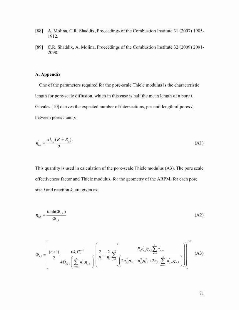
71

[88] A. Molina, C.R. Shaddix, Proceedings of the Combustion Institute 31 (2007) 1905-1912.

[89] C.R. Shaddix, A. Molina, Proceedings of the Combustion Institute 32 (2009) 2091-2098.

A. Appendix

One of the parameters required for the pore-scale Thiele modulus is the characteristic

length for pore-scale diffusion, which in this case is half the mean length of a pore i.

Gavalas [10] derives the expected number of intersections, per unit length of pores i,

between pores i and j:

0,',

( )

2j i j

i j

l R Rn

π += (A1)

This quantity is used in calculation of the pore-scale Thiele modulus (A3). The pore scale

effectiveness factor and Thiele modulus, for the geometry of the ARPM, for each pore

size i and reaction k, are given as:

,,

,

tanh( )i k

i k

i k

ηΦ

=Φ

(A2)

1/2

' '1 , , ,1

, 2 21 '2 '2 2 ' '

', , , , , , ,

, , ,1

1

( 1) 2 2

22 24

n

n j i j j k j mik k m i

i k nn ji i

j i i k j i i k j i j m m keff i i j j k

m ij i

R n nk Cn

R Rn n n nD n

ην

η η ηη

− −=

=

= += +

+ Φ = + − +

∑∑

∑∑

(A3)

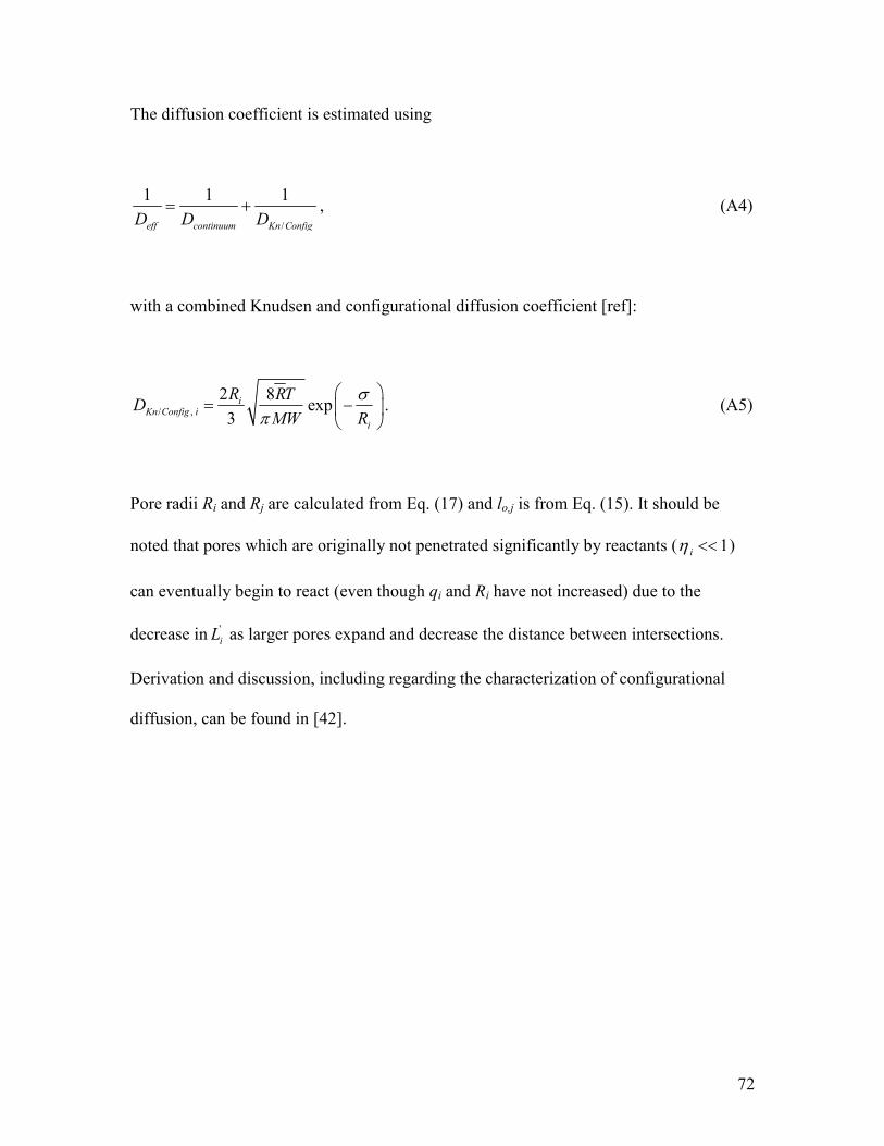
72

The diffusion coefficient is estimated using

/

1 1 1

eff continuum Kn ConfigD D D= + , (A4)

with a combined Knudsen and configurational diffusion coefficient [ref]:

/ ,

2 8exp

3i

Kn Config i

i

R RTD

MW R

σπ

= −

. (A5)

Pore radii Ri and Rj are calculated from Eq. (17) and lo,j is from Eq. (15). It should be

noted that pores which are originally not penetrated significantly by reactants ( 1iη << )

can eventually begin to react (even though qi and Ri have not increased) due to the

decrease in 'iL as larger pores expand and decrease the distance between intersections.

Derivation and discussion, including regarding the characterization of configurational

diffusion, can be found in [42].