Embed Size (px)
Citation preview

Computational UV/vis, IR and Raman Spectroscopy 1
1 Computer Experiment 8: Computational UV/vis, IR and Raman Spectroscopy
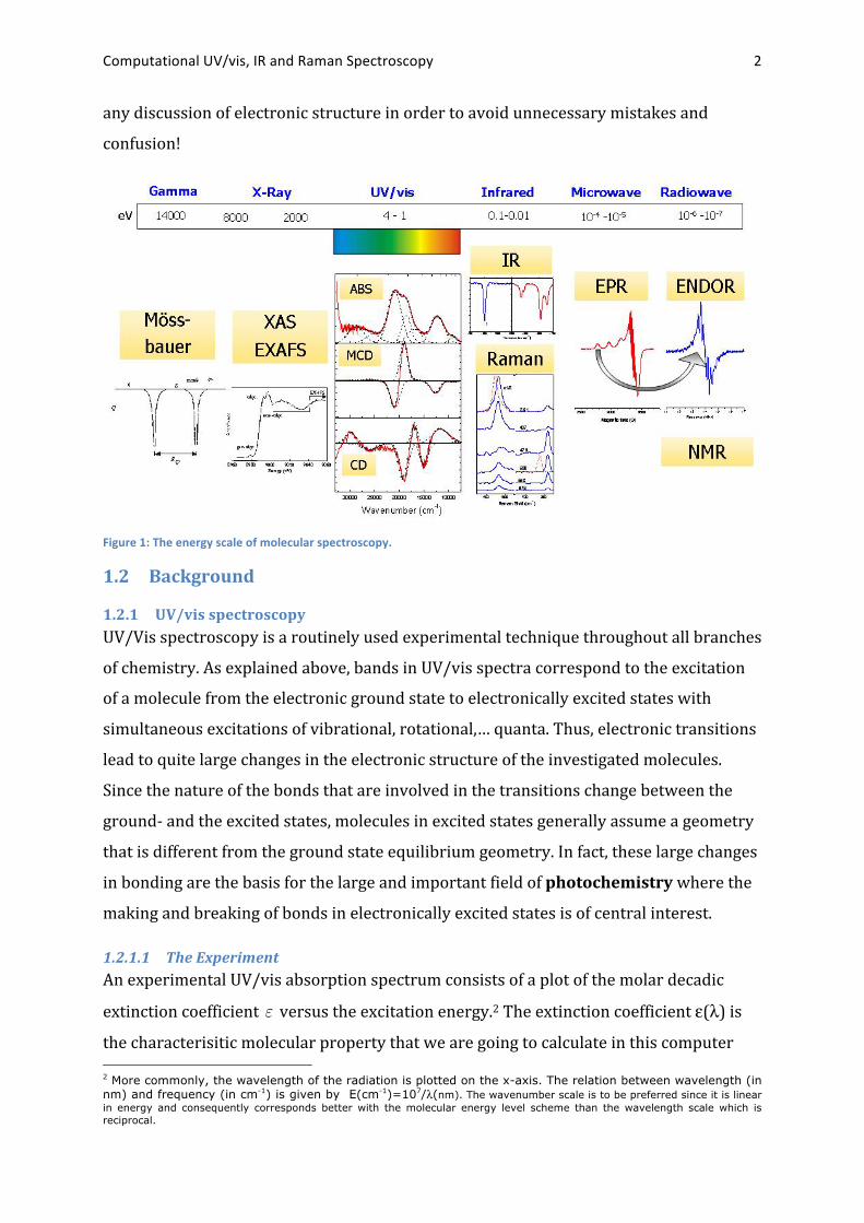
1.1 Introduction to Theoretical Spectroscopy Whenever it comes to the discussion of spectroscopy, it is essential to orient oneself
about the molecular phenomena that are being studied (Figure 1). The natural order
parameter for spectroscopy is the energy of the photons that are applied to the system.
For high energy gamma-‐ray photons (>104 eV) one studies nuclear processes (for
example in Mössbauer spectroscopy transition between different states of a 57Fe nucleus
are probed). Radiation in the hard-‐ and soft x-‐ray region (~104-‐102 eV) induces
electronic transitions from core-‐levels to empty valence levels or into the non-‐bound
continuum. Ultraviolet and visible (UV/vis) photons (1-‐4 eV) induce electronic
excitations from filled to empty valence (and perhaps Rydberg) levels. It is this energy
region where the photon energy is of the same order of magnitude than the energy of
chemical bonds. Thus, electronic spectroscopy directly probes chemical bonding! Below
the energy of visible photons, it is (usually) no longer possible to induce electronic
transitions. Thus, infrared photons (0.01-‐0.5 eV ~100-‐4000 cm-‐1) merely induce
transitions between different vibrational levels of the molecule within a given electronic
configuration.1 At even lower energy (10-‐4-‐10-‐5 eV; ~1-‐10 cm-‐1) there occur the
phenomena that are associated with the electron spin and that are probed by ESR (=EPR
for our purposes) spectroscopy. Finally, with radiowave photons (10-‐6-‐10-‐7~0.001-‐0.01
cm-‐1) one is only able to induce transitions between different states of magnetic nuclei
and these are probed in NMR (and ENDOR) spectroscopy.
In this computer experiment we study the UV/vis and infrared region of the spectrum
and calculate the energy levels that are associated in electronic and vibrational
transitions. In the next experiment, the low-‐energy region covered by magnetic
resonance spectroscopy is covered. In interpreting the results of the computations, we
will use the language of molecular orbitals. It is, however, very important to understand
that in actual experiments one never observes molecular orbitals. Every measurement
always only reports energies and properties of many electron states. It is crucial to
properly distinguish between the one-‐electron (MO) and many-‐electron (states) level in
1 An electronic configuration is defined by specifying the integer occupation number for each MO in the system such that the sum of occupation numbers equals the total number of electrons and each MO is occupied by either 0, 1 or 2 electrons.
Computational UV/vis, IR and Raman Spectroscopy 2
any discussion of electronic structure in order to avoid unnecessary mistakes and
confusion!
Figure 1: The energy scale of molecular spectroscopy.
1.2 Background
1.2.1 UV/vis spectroscopy UV/Vis spectroscopy is a routinely used experimental technique throughout all branches
of chemistry. As explained above, bands in UV/vis spectra correspond to the excitation
of a molecule from the electronic ground state to electronically excited states with
simultaneous excitations of vibrational, rotational,… quanta. Thus, electronic transitions
lead to quite large changes in the electronic structure of the investigated molecules.
Since the nature of the bonds that are involved in the transitions change between the
ground-‐ and the excited states, molecules in excited states generally assume a geometry
that is different from the ground state equilibrium geometry. In fact, these large changes
in bonding are the basis for the large and important field of photochemistry where the
making and breaking of bonds in electronically excited states is of central interest.
1.2.1.1 The Experiment An experimental UV/vis absorption spectrum consists of a plot of the molar decadic
extinction coefficient ! versus the excitation energy.2 The extinction coefficient ε(λ) is
the characterisitic molecular property that we are going to calculate in this computer 2 More commonly, the wavelength of the radiation is plotted on the x-axis. The relation between wavelength (in nm) and frequency (in cm-1) is given by E(cm-1)=107/λ(nm). The wavenumber scale is to be preferred since it is linear in energy and consequently corresponds better with the molecular energy level scheme than the wavelength scale which is reciprocal.
Computational UV/vis, IR and Raman Spectroscopy 3
experiment. The quantitative relation between absorbance, extinction coefficient,
concentration and pathlength is given by the Bourger-‐Lambert-‐Beer law. It is defined as
follows:
! =
A(")c !d
( 1)
where A =! log10(I I
0) is the measured absorbance, I0
is the intensity of the incident
light at a given wavelength ! , I is the transmitted intensity; c is the concentration (in
mol⋅l-‐1) and d is the pathlength (in cm). Broadly speaking, the electronic transition
energies correspond to absorption maxima in the UV/vis spectrum. The integral under
an absorption band characterizes the intensity of a given electronic transition. The
excitation energies may be given on the wavelength ( ! , in nm), frequency ( ! , in Hz),
wavenumber ( !! , in cm-‐1), eV, and atomic-‐unit scale (Eh). The reason for introducing the
wavelength, frequency and wavenumber as energy units in spectroscopy lies in the
Planck-‐Einstein relation between these parameters and the energy of incident photon:
E = h! = hcL/" = hc
L!! ( 2)
Here cL is the speed of light, and h is Planck’s constant. The conversion factors between
different energy units conventionally used in spectroscopy are given in Table 1 Table 1: Conversion factors between the energy units used in spectroscopy.
eV Hz cm-‐1 Eh eV 1 2.4179696×10¹⁴ 8.065479×10³ 3.674901×10-‐2 Hz 4.1357012×10-‐
15 1 3.3356412×10-‐
11 1.519829×10-‐
16 cm-‐1 1.239852×10-‐4 2.9979243×10¹⁰ 1 4.556333×10-‐6 Eh 27.21161 6.579686×10¹⁵ 2.194747×10⁵ 1
An absorption spectrum basically consists of a number of absorption bands. Each
absorption band corresponds to a transition of the ground-‐ electronic state to an excited
electronic state. For reasons to be discussed below, however, such transitions do not
take the appearance of sharp absorption lines (as in the spectra of atoms and ions) but
are usually considerably broadened. In many cases there will be overlapping bands and
one is faced with the problem of how to deconvolute the broad absorption envelope into
contributions from individual transitions. In most cases, one simply performs a “Gauss-‐
Fit”.3 That is, one assumes that the shape of each individual band is that of a Gaussian
3 This is an approximate procedure which is not without problems. First of all, accurate band-shapes do not follow the shapes of Gaussian functions. Secondly, the fits are often not well defined and unless one has
Computational UV/vis, IR and Raman Spectroscopy 4
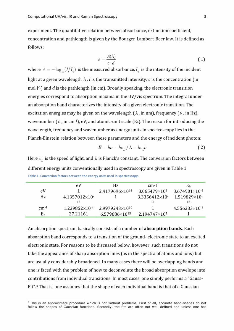
functions and then applies as many (or as few) Gaussian functions as are necessary in
order to accurately represent the absorption envelope. A typical example is shown in
Figure 2.
0
2
4
122
613
3
ε ( m
M -1
cm
-1 )
Δε
( M -1
cm
-1 )
-1.5
-1.0
-0.5
0.0
0.5
1.0
1.5
Δε ( m
M -1 cm
-1 )
2
9
10
12
10
3
6
9
12
30 25 20 15 10
-0.9
-0.6
-0.3
0.0
0.3
0.6
23
A.
B.
13
5
8
9
Wavelength (nm)
Wavenumber (1000 cm-1)
C.
350 550 750 9501150
Figure 2: Deconvolution of an absorption spectrum into contributions from individual electronic transitions using Gauss fits. The upper panel represents the absorption spectrum plotted on a wavenumber scale. The second panel represents the MCD spectrum and the lower panel the CD spectrum of the same compound. Note how the MCD and CD spectra help the deconvolution due to the fact that they are signed quantities.
Having obtained a reasonable Gauss-‐fit, it is possible to calculate the so-‐called oscillator
strength4 f0!I of the transition from the ground state to the I’th electronically excited
state. The oscillator strength is simply proportional to the area of the absorption band:
f0!I
=4.32 "10#9
n! I( )(!")d!"
Band$ ( 3)
(note that !I( )(!") is given in wavenumbers). The refractive index n is usually set equal
to one.
The phenomenon on electronic circular dichroism (CD) consists in that the left-‐handed
and right-‐handed circularly polarized light are not only propagated with different
velocities, but they are also absorbed to different extents in the region of an electronic
absorption band. This behavior is most simply described by the difference of the molar
additional information – for example from CD or MCD spectra – it is advisable to view the fit results with some caution. Additional Gaussians should not be used to improve the fits unless there is at least a well defined maximum or a well defined shoulder in the absorption envelope.
4 Its name stems from the classical dispersion theory and amounts to the number of virtual oscillators equivalent to a given transition.

Computational UV/vis, IR and Raman Spectroscopy 5
decadic absorption coefficients corresponding to the left-‐handed and right-‐handed
circularly polarized light !! = !L" !
R. Similar to the case of absorption the CD
spectrum can be deconvoluted into individual bands corresponding to different
electronic transitions. The fact that each electronic band in the CD signal can be of
positive or negative sign allows to resolve ambiguity in the spectral deconvolution. For
example, two stongly overlapping bands in an absorption spectrum can have different
signs in the corresponding CD spectrum, thus providing the evidence for two electronic
transitions in the given spectral range. Typically, CD spectra are analyzed together with
corresponding absorption spectra, since they arise from the same set of electronic
transitions. Each band in CD spectrum corresponding to the transition from the ground
state to the I’th electronically excited state is characterized by the the so-‐called rotatory
strength R0!I which is calculated as following
R
0!I= 0.229"10#38 $! I( )(!")
d!"!"Band% ( 4)
in units of esu2·cm2, where !! is in units of molar extinction coefficient.
1.2.1.2 Elementary Discussion of Electronic Transitions On a most elementary level, electronic transitions correspond to the transitions from
one electronic configuration to another. An example is shown in Figure 3. What is shown
there is the ground state electronic configuration of a square-‐planar transition metal-‐
dithiolene complex. It consists of a series of molecular orbitals that are drawn according
to increasing energy. According to the Aufbau principle, all MOs are filled by two
electrons and in the present case one unpaired electron remains and occupied a singly-‐
occupied MO (SOMO). The MOs transform under the irreducible representation of the
molecular point group and the symmetry labels are given for each MO.5
The many electron states found from distributing the electrons among the available
orbitals also have a symmetry that is designated by a term symbol. It is given by 2S+1Γ .
Here 2S+1 is the multiplicity of the electronic state (S is the total spin) and Γ is its
symmetry. In a nutshell, the symmetry is found by taking the direct product of all
partially occupied MOs. In general, this leads to a reducible representation of the
molecular point group. However, for non-‐degenerate point groups (D2h and subgroups),
5 Note that lowercase symbols are used to represent one-electron functions and uppercase symbols are used to represent many-electron states.

Computational UV/vis, IR and Raman Spectroscopy 6
the direct product directly yields the symmetry of the electronic state. In the example
above, a single b2g MO is singly occupied which leads to a 2B2g ground state.
Excited states are formed by promoting electrons from lower-‐lying orbitals into partially
occupied or empty MOs. For example, the transition 1b1u→2b2g leads to (1b1u)1(2b2g)2
which corresponds to a 2B1u excited state. Transition from 1au to 1b1g yields
(1au)1(1b2g)1(2b1g)1 which corresponds to an electron states au⊗b2g⊗b1g=2B3u. However,
this configuration has three unpaired electrons and consequently, it also gives rise to a 4B3u excited state. In order to distinguish different states of the same symmetry one
typically uses “X” for the ground state, the letters A,B,C for excited states of the same
multiplicity and a,b,c for excited states of different multiplity. Thus, in the present case,
we have identified a X-‐2B2g→A-‐2B1u and X-‐2B2g→B-‐2B3u transitions as well as a X-‐2B2g→a-‐4B3u transition.
Figure 3: Exemplification of electronic states and transitions. Shown is the ground state configuration with orbitals in order of decreasing energy (top to bottom). Excited states are essentially formed by promoting electrons from lower lying MOs into higher lying partially occupied or empty MOs.
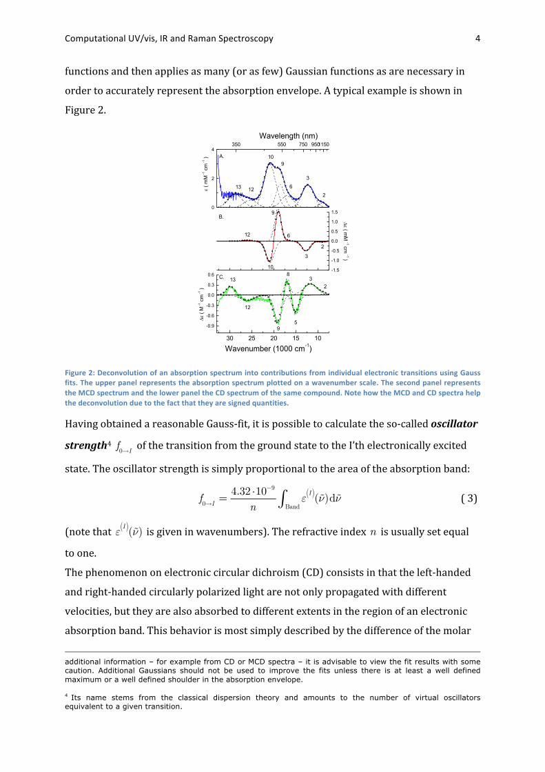
1.2.1.3 Selection Rules In order to perform an assignment of the electronic spectrum, it is necessary to
determine the symmetries of the excited states involved and identify the donor and
acceptor MO pairs involved in the transitions. A typical example is shown in Figure 4.
In order to find out whether an electronic transition is allowed or not, the following rules apply:
• Transitions between states of different multiplicity are forbidden. This is a fairly strong selection rule and such transitions typically have ε values < 1 M-‐1 cm-‐1.6
6 This selection rule is lifted by spin-orbit coupling. For heavier elements formally “spin-forbidden” transitions become increasingly allowed.
Computational UV/vis, IR and Raman Spectroscopy 7
• The direct product of the irreps of the initial and final states involved the transition with the irreps spanned by the electric dipole operator must contain the totally symmetric representation. Otherwise the transition is forbidden by symmetry.
The electric-‐dipole operator transforms like the molecular translations which can be
found with the labels “x”, “y” and “z” in usual group theoretical tables.7 As a consequence
of these rules:
• If the point group contains a center of inversion, only g→u transitions are
allowed (and vice versa). Other transitions are said to be “parity forbidden”.
The selection rules are a good guide to identifying strongly and weakly allowed
transitions in a spectrum. However, don’t be surprised to find a formally forbidden
transition in your spectrum. In the real world there are almost always additional
perturbations that break the symmetry of the system and make formally forbidden
transitions weakly allowed.8
0
1
2
3
4
MCDABS
calc
exp
8
7
6
54
3
287
65
42 -1
0
1exp
Δε
(mM
-1 c
m-1 T
-1)
ε (m
M-1 c
m-1)
25 20 15 100
1
2
3
calc
2a2g
3a1g
2b1g
1b3g
1b2g
1b1g1ag
2a2g
calc
Wavenumber (1000 cm-1)
3
25 20 15 10
-0.2
0.0
0.2calc
3ag2b1g
1b3g
1b2g
1b1g
1ag
2a2g
Figure 4: An example for an assigned absorption spectrum. The experimental absorption and MCD spectra are given in the upper panel and calculated spectra are shown in the lower panel. The acceptor MO is always a b3u level in this case and the lowercase symbols on the calculated transitions merely represent the symmetry of the donor MO. The theoretical calculations yield “only” the black bars in the lower panels which have been empirically convoluted by
7 The most popular text in chemistry is F.A. Cotton: Chemical Applications of Group Theory, John Wiley and Sons, New York, 1990. It has very useful tables. A more theoretically oriented text is R. McWeeny Symmetry – An introduction to Group Theory and Its Applications. Dover, New York, 2002.
8 A typical example are the parity forbidden d-d transitions studied in chapter Error! Reference source not
found..

Computational UV/vis, IR and Raman Spectroscopy 8
Gaussian functions in order to produce an envelope that can be compared with the experimental measurement. For this example see9
Since the rotational strength of a transition is proportional to the scalar product of the
electric and magnetic dipole transition moments (see the next section) the selection
rules are different than those for the case of normal absorption. Since g→g and u→u
transitions are formally electric forbidden, whereas g→u and u→g are magnetic dipole
forbidden, it is immidiatley apperent that centrosymmetric molecules are not optically
active. More generally, it can be shown that a molecule must lack any Sn axis (including
S1! ! and S2
! i ) to be optically active, which translates to only those molecules with
nonsuperimpsable mirror images. Such molecules are called chiral. Enantiomers, which
are stereoisomers that are nonsuperimposable complete mirror images of each other,
show CD signals of equal amplitudes but different signs. Only molecules belonging to the
point groups Cn, Dn
, O , T , or I are optically active and discrete transitions must be
both electric and magnetic dipole allowed to exhibit CD .
1.2.1.4 Refined Discussion of Electronic Transitions In this section, we will purse a slightly more “physical” description of the aborption
processes that leads the way towards a more quantitative description of the spectra. The
theoretical description of the absorption process rests on two major assumptions: The
first assumption is to assume that the strength of the external electromagnetic field
(provided by the electromagnetic wave) is much smaller than the electric fields that act
“inside” the molecules. In such a case the external electromagnetic force can be reliably
modeled as a small perturbation. In this case, the radiation may be described as a time-‐
dependent electromagnetic field and the vast majority of observable electronic
transitions are well interpreted within the first-‐order time-‐dependent perturbation
treatment. Secondly, it is assumed that the wavelength of light is much larger than the
dimensions of the investigated molecules. Thus, the oscillating electromagnetic field is
assumed to be essentially uniform over the extension of the molecule. This is the essence
of the so-‐called electric-‐dipole approximation.
Both assumptions can and need to be refined in special circumstances, like very intense
electromagnetic fields provided by lasers or very short wavelengts used in X-‐ray
9 Neese, F.; Zumft, W.G.; Antholine, W.E.; Kroneck, P.M.H.; (1996) J. Am. Chem. Soc., 118, 8692-8699; Farrar, J.; Neese, F.; Lappalainen, P.; Kroneck, P.M.H.; Saraste, M.; Zumft, W.G.; Thomson, A.J. (1996) J. Am. Chem. Soc. 118:11501-11514.
Computational UV/vis, IR and Raman Spectroscopy 9
absorption spectroscopy. Taking into account higher-‐order terms in the time-‐dependent
perturbation approach leads to multi-‐photon non-‐linear processes, for which molecular
transitions occur with simultaneous absorption of two and more photons. There are also
corrections to the long-‐wavelength approximation that describe magnetic dipole,
electric quadrupole and higher-‐order multipole transitions which usually give rise to
low-‐intensity spectral lines in ordinary experiments.
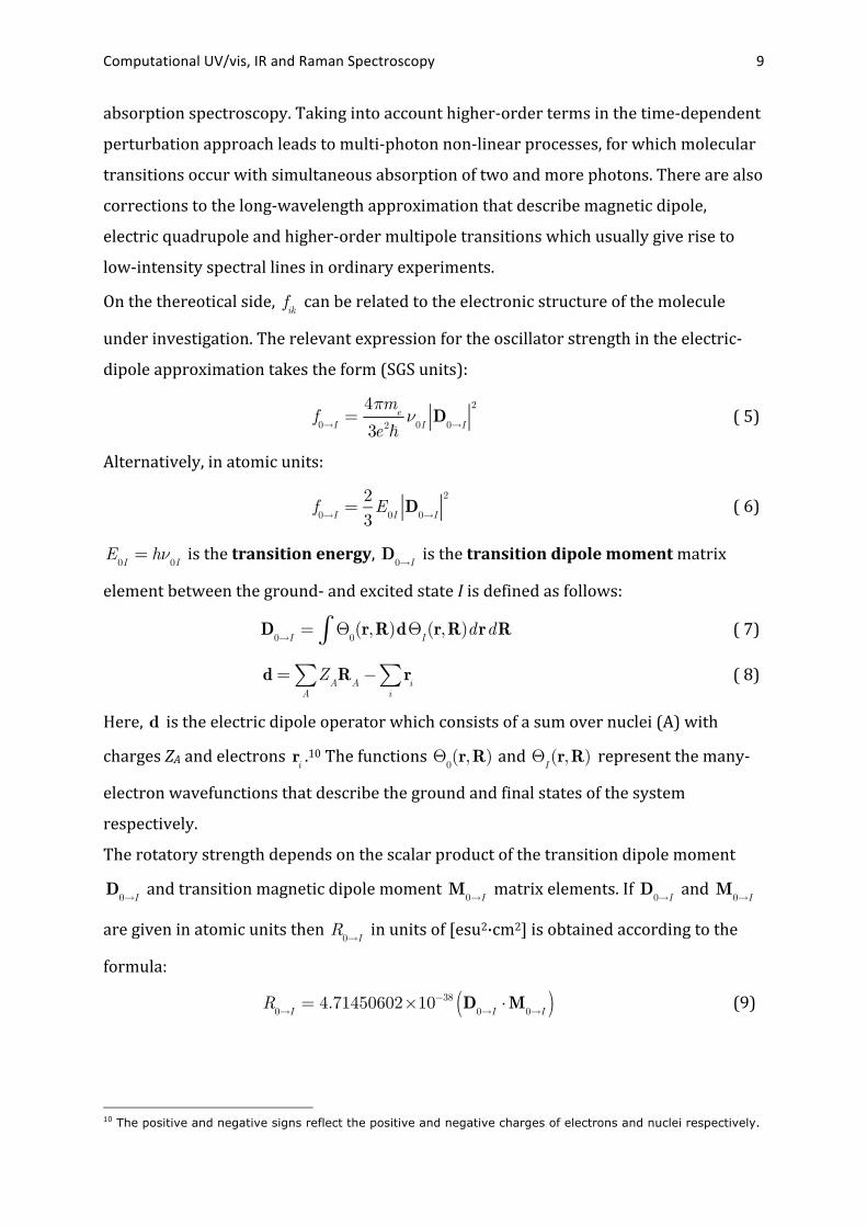
On the thereotical side, fik can be related to the electronic structure of the molecule
under investigation. The relevant expression for the oscillator strength in the electric-‐
dipole approximation takes the form (SGS units):
f0!I
=4!m
e
3e2!"
0ID
0!I
2 ( 5)
Alternatively, in atomic units:
f0!I
=23E
0ID
0!I
2 ( 6)
E0I= h!
0I is the transition energy, D0!I
is the transition dipole moment matrix
element between the ground-‐ and excited state I is defined as follows:
D
0!I= "
0(r,R)d"
I(r,R)drdR# ( 7)
d = Z
AR
AA! " r
ii! ( 8)
Here, d is the electric dipole operator which consists of a sum over nuclei (A) with
charges ZA and electrons ri .10 The functions !0
(r,R) and !I(r,R) represent the many-‐
electron wavefunctions that describe the ground and final states of the system
respectively.
The rotatory strength depends on the scalar product of the transition dipole moment
D0!I and transition magnetic dipole moment M0!I
matrix elements. If D0!I and M0!I
are given in atomic units then R0!I in units of [esu2·cm2] is obtained according to the
formula:
R
0!I= 4.71450602"10#38 D
0!I$M
0!I( ) (9)
10 The positive and negative signs reflect the positive and negative charges of electrons and nuclei respectively.
Computational UV/vis, IR and Raman Spectroscopy 10
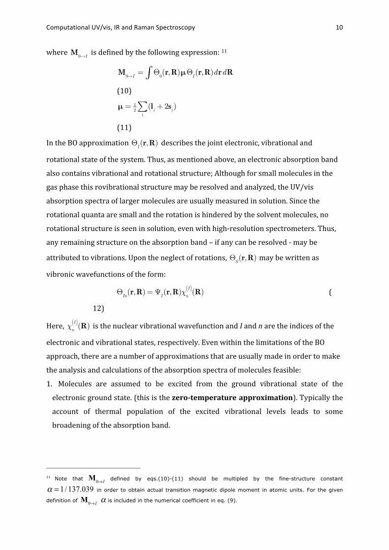
where M0!I is defined by the following expression: 11
M
0!I= "
0(r,R)µ"
I(r,R)drdR#
(10)
µ = 1
2(l
i+ 2s
i)
i!
(11)
In the BO approximation !I(r,R) describes the joint electronic, vibrational and
rotational state of the system. Thus, as mentioned above, an electronic absorption band
also contains vibrational and rotational structure; Although for small molecules in the
gas phase this rovibrational structure may be resolved and analyzed, the UV/vis
absorption spectra of larger molecules are usually measured in solution. Since the
rotational quanta are small and the rotation is hindered by the solvent molecules, no
rotational structure is seen in solution, even with high-‐resolution spectrometers. Thus,
any remaining structure on the absorption band – if any can be resolved -‐ may be
attributed to vibrations. Upon the neglect of rotations, !S(r,R) may be written as
vibronic wavefunctions of the form:
!In(r,R) = "
I(r,R)!
n
I( )(R) (
12)
Here, !n
I( )(R) is the nuclear vibrational wavefunction and I and n are the indices of the
electronic and vibrational states, respectively. Even within the limitations of the BO
approach, there are a number of approximations that are usually made in order to make
the analysis and calculations of the absorption spectra of molecules feasible:
1. Molecules are assumed to be excited from the ground vibrational state of the
electronic ground state. (this is the zero-‐temperature approximation). Typically the
account of thermal population of the excited vibrational levels leads to some
broadening of the absorption band.
11 Note that M0!I defined by eqs.(10)-(11) should be multipled by the fine-structure constant
! = 1/ 137.039 in order to obtain actual transition magnetic dipole moment in atomic units. For the given
definition of M0!I ! is included in the numerical coefficient in eq. (9).
Computational UV/vis, IR and Raman Spectroscopy 11
2. The electronic transition dipole moment defined as
d
0I(R) = !
0(r,R)d!
I(r,R)dr" does not depend upon nuclear coordinates, and equal
to the value corresponding to the ground-‐state equilibrium geometry R0:
d0I(R)! d
0I(R
0) = const . This statement constitutes the essence of the so-‐called
Franck-‐Condon approximation.
3. Due to the vibronic nature of the molecular states the excitation of the 0! k
electronic transition implies a co-‐excitation of of vibrational quanta from the ground
vibrational state of the electronic ground state into the ground-‐ and excited vibrational
states on the k’th electronic state. For a given electronic transition 0! k the excitation
of the vibrational quanta in a given normal mode constitute a vibrational progression.
In the general case, the intensity distribution within such a progression corresponding
to transitions of the form !0(r,R)!
0
0( )(R)" !I(r,R)!
n
I( )(R) is determined by the square
of the vibrational-‐overlap integrals !
0
0( ) !n
I( )2
(Franck-‐Condon factors). Their
precise calculation for larger molecules and realistic PESs is a quite complicated
problem and calls for further simplifications. The Franck-‐Condon (FC) principle states
that the electronic ground-‐state vibrational wavefunction !0
0( )(R) has large overlap
with the excited-‐state wavefunctions !n
I( )(R) only if their energy levels are close to the
vertical transition. The vertical transition occurs when the molecule is promoted from
the electronic ground state to the electronically excited state at the ground state
equilibrium geometry (Figure 5).12
1.2.1.5 Vibrational Fine Structure Although the absorption spectra of various chemical species are characterized by
vibrational structure, the latter is frequently obscured due to intermolecular collisions,
solvent effects and spectral crowding. In such a case and absorption band may be viewed
as the envelope of different vibronic transitions (Figure 5). Its intensity (area under the
absorption band) is given by the oscillator strength. The simultaneous neglect of
vibrational and rotation finestructure together with the zero-‐temperature and Franck-‐
Condon approximation on harmonic potential energy surfaces present the most
12 The FC principle can be rigorously derived only for diatomic harmonic PES’s and for many-atom molecules and more complicated shapes of the PESs it should be used with caution.

Computational UV/vis, IR and Raman Spectroscopy 12
simplified level of theoretical description. It only requires the knowledge of the energies
and electronic wavefunctions of the ground and excited states which are all evaluated at
the ground-‐state equilibrium geometry. Despite the many simplifying assumptions this
already represents a very useful level of theory.
The prediction of the vibrational structure of the absorption spectra is based on the
calculations of vibrational-‐overlap integrals !
0
0( ) !n
I( )2
which in general case depend in
a very complicated way on the shape of PES’s. However, under the simplifying
assumption of harmonic potentials, the problem can be solved exactly. In this case the
distribution of intensity between various vibronic bands only depends on the
equilibrium shift,13 frequency alteration14 and normal mode rotation in the excited
state,15 such that the entire absorption bandshape can be written in the closed form as a
function of these parameters. Of these factors, only the first one – the equilibrium shift –
is of major importance. The neglect of the normal mode rotations leads to the
Independent Mode Displaced Harmonic Oscillator (IMDHO) model. In this simplified
framework, the vibrational progression is determined solely by the equilibrium shift and
vibrational frequency alteration between the ground-‐ and excited-‐state PES’s.16
13 The quantities Δ are defined above
14 The change of vibrational frequencies in the excited state due to the change of bonding.
15 This is a fairly complicated effect known as “Duschinsky rotation”. Is arises from the fact that the force field of the molecule is different for each electronic state. Thus, the shapes of normal modes also change from state to state which leads to additional complexity in the calculation of FC factors.
16 For a detailed recent discussion see Petrenko, T.; Neese, F. (2007) Analysis and Prediction of Absorption Bandshapes, Fluorescence Bandshapes, Resonance Raman Intensities and Excitation Profiles using the Time Dependent Theory of Electronic Spectroscopy. J. Chem. Phys., 127, 164319; Neese, F.; Petrenko, T.; Ganyushin, D.; Olbrich, G. (2007) Advanced Aspects of ab initio Theoretical Spectroscopy of Open-Shell Transition Metal Ions. Coord. Chem. Rev., 205, 288-327.
Computational UV/vis, IR and Raman Spectroscopy 13
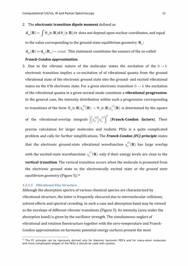
Figure 5: Illustration of the Franck-‐Condon principle. The excitation into electronic band involves the coexcitation of vibrational levels which results in the vibrational progression of the absorption. The vibronic peak of maximum intensity corresponds to the excited-‐state vibrational level which is most close to the intersection of the vertical transition (red line) with the excited-‐state PES. As a result the maximum of the broadened absorption spectrum occurs close to the vertical transition energy. For the IMDHO model the number of intense peaks in the absorption progression correlates with the value of Δ.
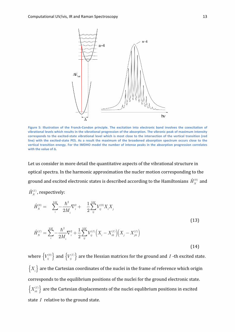
Let us consider in more detail the quantitative aspects of the vibrational structure in
optical spectra. In the harmonic approximation the nucler motion corresponding to the
ground and excited electronic states is described according to the Hamiltonians HN
(0) and
HN
(I ) , respectively:
H
N
(0) = !!2
2Mii
3M
" #i
2 +12
Vij
(0)X
iX
j
ij
3M
"
(13)
H
N
(I ) = !!2
2Mii
3M
" #i
2 +12
Vij
(I )X
i!X
i0(I )( ) X
j!X
j 0(I )( )
ij
3M
"
(14)
where V
ij(0){ } and Vij
(I ){ } are the Hessian matrices for the ground and I -‐th excited state.
X
i{ } are the Cartesian coordinates of the nuclei in the frame of reference which origin corresponds to the equilibrium positions of the nuclei for the ground electronic state.
X
i0(I ){ } are the Cartesian displacements of the nuclei equlibrium positions in excited
state I relative to the ground state.
Computational UV/vis, IR and Raman Spectroscopy 14
Note, that if HN
(0) and HN
(I ) are identical, i.e. V
ij(I ) =V
ij(0) and Xi0
(I ) = 0 for all i , j , then the
ground-‐ and excited-‐state vibrational Hamiltonians are characterized by the common set
of vibrational eigenfunctions, so that !
0
0( ) !0
I( ) = 1 , whreas all other integrals
!
0
0( ) !n
I( ) = 0 . As soon as the equilibrium positions of atoms in the excited state are
changed compared to the ground state ( Xi0(I ) ! 0 ), and/or there is a change in the force
constants V
ij(I ) !V
ij(0) , then
!
0
0( ) !0
I( ) <1 , and there will be certain vibrational levels !n
I( )
for which !
0
0( ) !n
I( ) ! 0 . This means that one would observe different transitions
between the ground vibrational level in the ground state and various vibrational levels
corresponding to the excited state. The intensity pattern of such a vibrational structure
depends in a rather complicated way on the difference between HN
(0) and HN
(I ) .
Upon appropriate linear transformation from Cartesian to normal coordinates it is
possible to obtain decoupled representation of HN
(0) and HN
(I ) , which eigenfunctions are
the products of one-‐dimensional Hermitian functions of normal coordinates.
Consider particular case V
ij(I ) =V
ij(0) =V
ij for all i , j , for which, as can be shown, there is
no change in vibrational frequencies and shapes of normal modes between the ground
and excited states. Let us assume also that the equilibrium positions of atoms in the
excited state are changed compared to the ground state ( Xi0(I ) ! 0 ). A given vibrational
state !n
I( ) is completely determined by a set
n!{ } of occupation numbers for individual
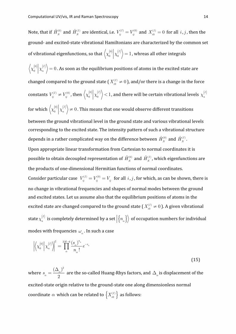
modes with frequencies !" . In such a case
!
0
0( ) !n
I( )2
=(s")n"
n"!
e!s"
"
3M!6
"
(15)
where s!
=(!
!)2
2 are the so-‐called Huang-‐Rhys factors, and !! is displacement of the
excited-‐state origin relative to the ground-‐state one along dimensionless normal
coordinate ! which can be related to X
i0(I ){ } as follows:
Computational UV/vis, IR and Raman Spectroscopy 15
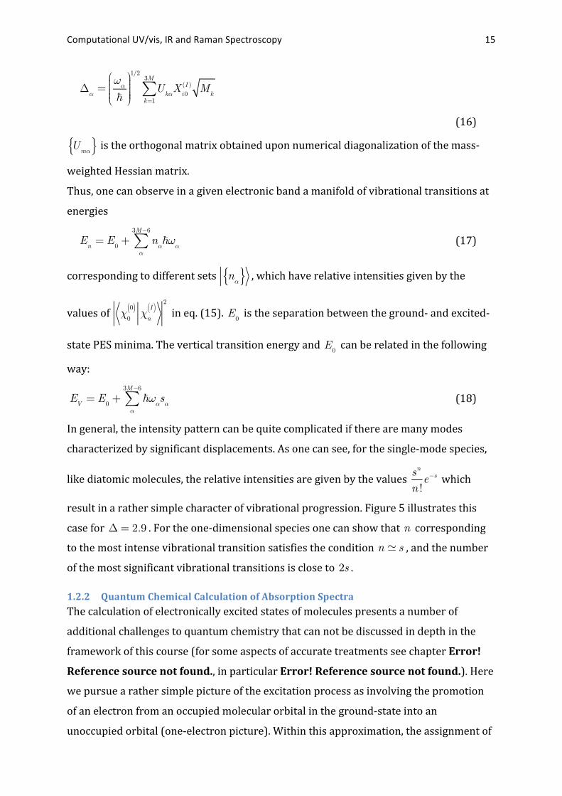
!!
="!
!
"
#$$$$
%
&'''''
1/2
Uk!
Xi0(I ) M
kk=1
3M
(
(16)
U
m!{ } is the orthogonal matrix obtained upon numerical diagonalization of the mass-‐weighted Hessian matrix.
Thus, one can observe in a given electronic band a manifold of vibrational transitions at
energies
E
n= E
0+ n
!!"!
!
3M!6
" (17)
corresponding to different sets
n!{ } , which have relative intensities given by the
values of !
0
0( ) !n
I( )2
in eq. (15). E0 is the separation between the ground-‐ and excited-‐
state PES minima. The vertical transition energy and E0 can be related in the following
way:
E
V= E
0+ !!
"s"
"
3M!6
" (18)
In general, the intensity pattern can be quite complicated if there are many modes
characterized by significant displacements. As one can see, for the single-‐mode species,
like diatomic molecules, the relative intensities are given by the values
sn
n !e!s which
result in a rather simple character of vibrational progression. Figure 5 illustrates this
case for != 2.9 . For the one-‐dimensional species one can show that n corresponding
to the most intense vibrational transition satisfies the condition n ! s , and the number
of the most significant vibrational transitions is close to 2s .
1.2.2 Quantum Chemical Calculation of Absorption Spectra The calculation of electronically excited states of molecules presents a number of
additional challenges to quantum chemistry that can not be discussed in depth in the
framework of this course (for some aspects of accurate treatments see chapter Error!
Reference source not found., in particular Error! Reference source not found.). Here
we pursue a rather simple picture of the excitation process as involving the promotion
of an electron from an occupied molecular orbital in the ground-‐state into an
unoccupied orbital (one-‐electron picture). Within this approximation, the assignment of
Computational UV/vis, IR and Raman Spectroscopy 16
an absorption spectrum consists of the determination which donor and acceptor MOs
give the dominant contribution to the observed absorption bands as exemplified above.
In general, this picture is oversimplified since the excited state is usually not well
represented in terms of a single Slater determinant and secondly, the orbitals of the
ground state will not be appropriate for the electronically excited state. Nevertheless,
the simplest reasonable approximation is to write the ground state as a single
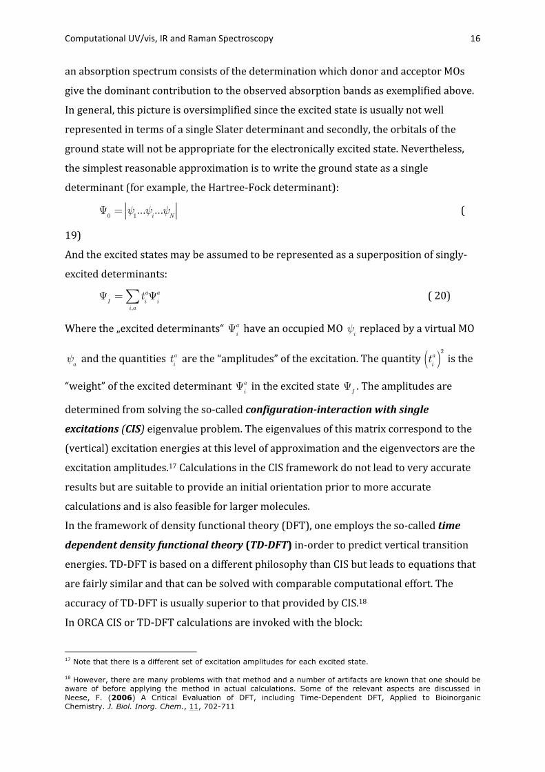
determinant (for example, the Hartree-‐Fock determinant):
!
0= !
1...!
i...!
N (
19)
And the excited states may be assumed to be represented as a superposition of singly-‐
excited determinants:
!
I= t
ia!
ia
i,a" ( 20)
Where the „excited determinants“ !ia have an occupied MO !i
replaced by a virtual MO
!a and the quantities ti
a are the “amplitudes” of the excitation. The quantity tia( )2 is the
“weight” of the excited determinant !ia in the excited state !I
. The amplitudes are
determined from solving the so-‐called configuration-‐interaction with single
excitations (CIS) eigenvalue problem. The eigenvalues of this matrix correspond to the
(vertical) excitation energies at this level of approximation and the eigenvectors are the
excitation amplitudes.17 Calculations in the CIS framework do not lead to very accurate
results but are suitable to provide an initial orientation prior to more accurate
calculations and is also feasible for larger molecules.
In the framework of density functional theory (DFT), one employs the so-‐called time
dependent density functional theory (TD-‐DFT) in-‐order to predict vertical transition
energies. TD-‐DFT is based on a different philosophy than CIS but leads to equations that
are fairly similar and that can be solved with comparable computational effort. The
accuracy of TD-‐DFT is usually superior to that provided by CIS.18
In ORCA CIS or TD-‐DFT calculations are invoked with the block:
17 Note that there is a different set of excitation amplitudes for each excited state.
18 However, there are many problems with that method and a number of artifacts are known that one should be aware of before applying the method in actual calculations. Some of the relevant aspects are discussed in Neese, F. (2006) A Critical Evaluation of DFT, including Time-Dependent DFT, Applied to Bioinorganic Chemistry. J. Biol. Inorg. Chem., 11, 702-711
Computational UV/vis, IR and Raman Spectroscopy 17
For HF reference wavefunction (RHF or UHF) the program automatically chooses CIS
calculations and for DFT model (RKS or UKS) TD-‐DFT. Below is a summary of variables
that can be assigned within the block:
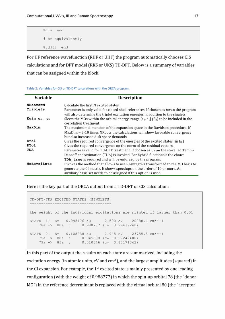
Table 2: Variables for CIS or TD-‐DFT calculations with the ORCA program.
Variable Description NRoots=N Calculate the first N excited states Triplets Parameter is only valid for closed shell references. If chosen as true the program
will also determine the triplet excitation energies in addition to the singlets Ewin e0, e1 Slects the MOs within the orbital energy range [e0, e1] (Eh) to be included in the
correlation treatment MaxDim The maximum dimension of the expansion space in the Davidson procedure. If
MaxDim ≈ 5-‐10 times NRoots the calculations will show favorable convergence but also increased disk space demands
Etol Gives the required convergence of the energies of the excited states (in Eh) RTol Gives the required convergence on the norm of the residual vectors. TDA Parameter is valid for TD-‐DFT treatment. If chosen as true the so-‐called Tamm-‐
Dancoff approximation (TDA) is invoked. For hybrid functionals the choice TDA=true is required and will be enforced by the program.
Mode=riints Invokes the method that allows to use RI-‐integrals transformed to the MO basis to generate the CI matrix. It shows speedups on the order of 10 or more. An auxiliary basis set needs to be assigned if this option is used.
Here is the key part of the ORCA output from a TD-‐DFT or CIS calculation:
In this part of the output the results on each state are summarized, including the
excitation energy (in atomic units, eV and cm-‐1), and the largest amplitudes (squared) in
the CI expansion. For example, the 1st excited state is mainly presented by one leading
configuration (with the weight of 0.988777) in which the spin-‐up orbital 78 (the “donor
MO”) in the reference determinant is replaced with the virtual orbital 80 (the “acceptor
%cis end # or equivalently %tddft end
------------------------------------ TD-DFT/TDA EXCITED STATES (SINGLETS) ------------------------------------ the weight of the individual excitations are printed if larger than 0.01 STATE 1: E= 0.095176 au 2.590 eV 20888.6 cm**-1 78a -> 80a : 0.988777 (c= 0.99437248) STATE 2: E= 0.108238 au 2.945 eV 23755.5 cm**-1 79a -> 80a : 0.945608 (c= -0.97242400) 79a -> 83a : 0.010346 (c= 0.10171342)

Computational UV/vis, IR and Raman Spectroscopy 18
MO”); the symbol “a” in the output next to the orbital number means that this is a spin-‐
up orbital; alternatively, “b” corresponds to spin-‐down orbitals.
Transition energies and oscillator strengths for the calculated excited states are given in
the following part of the output:
The column fosc shows calculated oscillator strengths. TX, TY, TZ are the components
of electronic transition dipole moment (in atomic unit), T2 is the square of transition
moment.
The output of rotatory strengths for the calculated excited states has similar structure:
The column R shows calculated rotatory strengths. MX, MY, MZ are the components of
electronic transition dipole moment (in atomic unit).
If you want to obtain a plot of the absorption spectrum then call the small utility
program orca_mapspc:
The program will produce outputfile.abs.dat file containing absorption
spectrum that can be plotted with standard graphics programs. Options are explained
here:
-x0value Start of the x-‐axis for the plot -x1value End of the x-‐axis for the plot -wvalue Full-‐width at half-‐maximum height in cm-‐1 for each transition
----------------------------------------------------------------------------- ABSORPTION SPECTRUM ------------------------------------------------------------------------------ State Energy Wavelength fosc T2 TX TY TZ (cm-1) (nm) (au**2) (au) (au) (au) ------------------------------------------------------------------------------ 1 20888.6 478.7 0.094387411 1.48758 0.08858 -1.21644 -0.00006 2 23755.5 421.0 0.167847587 2.32609 -0.00002 -0.00013 -1.52515 3 32083.8 311.7 0.295677742 3.03395 0.13992 1.73619 0.00009
----------------------------------------------------------------------------- CD SPECTRUM ------------------------------------------------------------------------------ State Energy Wavelength R MX MY MZ (cm-1) (nm) (1e40*cgs) (au) (au) (au) ------------------------------------------------------------------------------ 1 20888.6 478.7 3.659617854 0.32713 0.01744 -0.00002 2 23755.5 421.0 -166.793655155 0.96929 -0.50766 0.23200 3 32083.8 311.7 329.282848783 0.42056 0.36840 -0.12245
orca_mapspc outputfile abs –x015000 –x135000 –w200 –n2000
Computational UV/vis, IR and Raman Spectroscopy 19
-nvalue Number of points to be used
Thus, in the above example the absorption spectrum will be produced for 2000
equidistant points in the range 15000-‐35000 cm-‐1 using full-‐width at half-‐maximum
height equal to 200 cm-‐1 for each transition.
Likewise, CD plot can be obtained by calling orca_mapspc with another option:
The program will produce outputfile.cd.dat file containing CD spectrum.
1.2.3 IR and Raman spectroscopy
1.2.3.1 Normal Modes and Vibrational Frequencies Infrared (IR) and Raman spectroscopies are mutually complementary parts of molecular
vibrational spectroscopy. Their molecular physics is essentially the same since both are
concerned with the observation of the excitation of molecular vibrational energy states
associated with the electronic ground-‐state PES. In IR spectroscopy, vibrational
excitations occur upon the absorption of electromagnetic radiation. In Raman
measurements the excitation is a consequence of inelastic light scattering by molecule.
Upon the assumption that the PES is quadratic in atomic displacements (harmonic
model) the vibrational states of an M-‐atom molecule are described as a superposition of
3M-‐6 (3M-‐5 for linear molecules) independent harmonic oscillators which describe the
collective harmonic vibrational motion of the nuclei about their equilibrium
configuration. The shapes of different vibrations are characterized by different patterns
of the joint nuclear displacements and are called normal modes (coordinates).19 They
transform under the irreducible representations of the molecular symmetry group and
may therefore be classified by their symmetry. The textbook example of the H2O
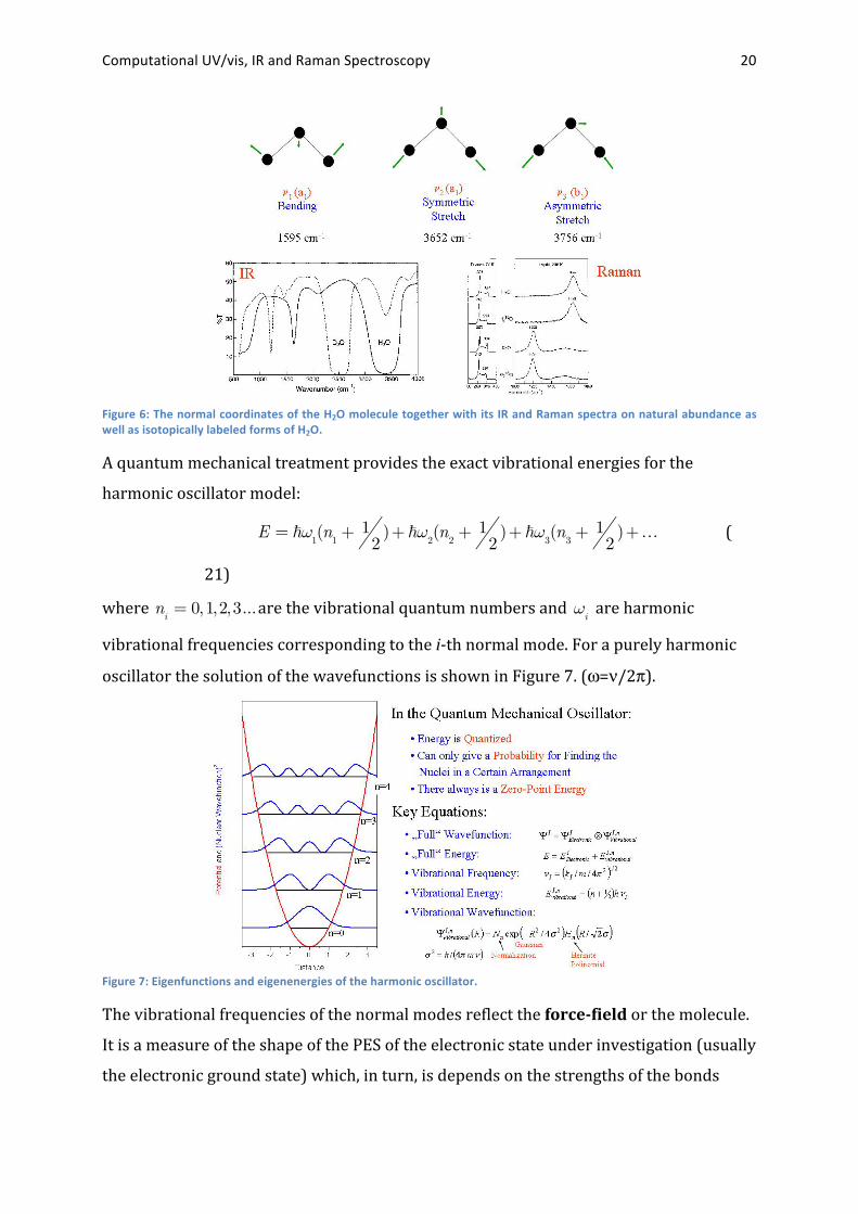
molecule is shown in Figure 6.20
19 Their construction will not be pursued in this course.
20 Still the most popular book that describes the calculation and use of normal coordinates from force fields in detail is classic text: Wilson, E.B.; Decius, J.C.; Cross, P.C. Molecular Vibrations – The Theory of Infrared and Raman Spectra, Dover, New York, 1980; the original text is from 1955.
orca_mapspc outputfile cd –x015000 –x135000 –w200 –n2000
Computational UV/vis, IR and Raman Spectroscopy 20
Figure 6: The normal coordinates of the H2O molecule together with its IR and Raman spectra on natural abundance as well as isotopically labeled forms of H2O.
A quantum mechanical treatment provides the exact vibrational energies for the
harmonic oscillator model:
E = !!
1(n
1+ 1
2)+ !!
2(n
2+ 1
2)+ !!
3(n
3+ 1
2)+… (
21)
where ni= 0,1,2,3...are the vibrational quantum numbers and !i
are harmonic
vibrational frequencies corresponding to the i-‐th normal mode. For a purely harmonic
oscillator the solution of the wavefunctions is shown in Figure 7. (ω=ν/2π).
Figure 7: Eigenfunctions and eigenenergies of the harmonic oscillator.
The vibrational frequencies of the normal modes reflect the force-‐field or the molecule.
It is a measure of the shape of the PES of the electronic state under investigation (usually
the electronic ground state) which, in turn, is depends on the strengths of the bonds

Computational UV/vis, IR and Raman Spectroscopy 21
between the different nuclei. For a diatomic molecule, the force constant k is simply the
second derivative of the electronic energy at the equilibrium distance:
k =!2E I( )
!R2
R=R
(
22)
From which the vibrational frequency is readily calculated as:21
! =
12"c
km (
23)
Where the reduced mass m is defined in Figure 8 below.
Figure 8: Vibrations of a diatomic molecule.
For a general polyatomic molecule, the definition of the force constant must be
generalized. It is replaced by the Hessian matrix already used extensively in the
previous computer experiments. Its definition is:
HAB
=!2
EI( )
!XA!X
BX
A=X
B=...X
(
24)
(XA, XB,… are Cartesian coordinates of atoms A,B,…) Essentially, diagonalization of the
mass weighted Hessian matrix ( !HAB
= HAB
mAm
B( )"1/2
) yields the normal modes and
harmonic vibrational frequencies of the system.
21 For correct units and conversion factors see chapter Error! Reference source not found.
Computational UV/vis, IR and Raman Spectroscopy 22
1.2.3.2 Selection Rules The important difference between IR and Raman spectroscopies is that for non-‐zero IR
intensity there must be a change of dipole moment along a given normal mode. For
diatomic molecules, this means that they must have a permanent dipole moment in
order to be IR active. For nonzero Raman intensities there must be a change in the
polarizability during the vibration.
Taking into account only linear terms in variations of dipole moment (for IR) and
polarizability (for Raman) during the vibration leads to the vibrational selection rule for
harmonic case. It states that only excitations with !n = ±1 in only one single mode are
allowed upon the vibrational transition. For such a case, IR and Raman spectra consist
only of fundamental transitions at the frequencies which coincide with the vibrational
harmonic frequencies of the molecule. The use of group theory and symmetry
arguments can be of great assistance in determining of which vibrations are IR or
Raman active and which are not. Character tables for the various symmetry groups can
be used to predict how many of the 3N-‐6 vibrations are IR active and how many are
Raman active. In particular, if the symmetry point group possesses a center of inversion,
there is a mutual exclusion rule which states that vibrations allowed in the Raman
spectrum are forbidden in IR, and vice versa. The symmetry of a molecule may also
dictate that certain bands are forbidden in both the IR and Raman spectra, in which case
even the combination of the two spectra will not provide the full information about the
3N-‐6 normal frequencies.
1.2.3.3 Anharmonicities A more detailed treatment of the vibrational spectra of molecules can be made if
anharmonicity is included into consideration. In this case the quadratic model for PES
function is extended by cubic and higher-‐power terms.22 The occurance of
anharmonicities has several important consequences for vibrational spectroscopy.
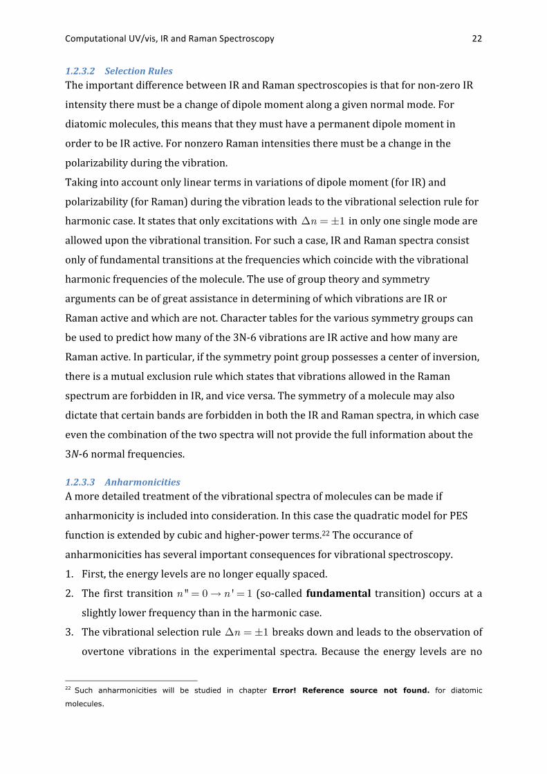
1. First, the energy levels are no longer equally spaced.
2. The first transition n '' = 0! n ' = 1 (so-‐called fundamental transition) occurs at a
slightly lower frequency than in the harmonic case.
3. The vibrational selection rule !n = ±1 breaks down and leads to the observation of
overtone vibrations in the experimental spectra. Because the energy levels are no
22 Such anharmonicities will be studied in chapter Error! Reference source not found. for diatomic
molecules.
Computational UV/vis, IR and Raman Spectroscopy 23
longer equidistant, the positions of the overtones are not given by integer multiples
of the fundamental frequency n '' = 0! n ' = 1 .
4. In addition to overtones, combination bands become weakly allowed in which two
different vibrational modes are simultaneously excited.
Figure 9: Description of overtone, combination and “hot” bands in IR and Raman spectra.
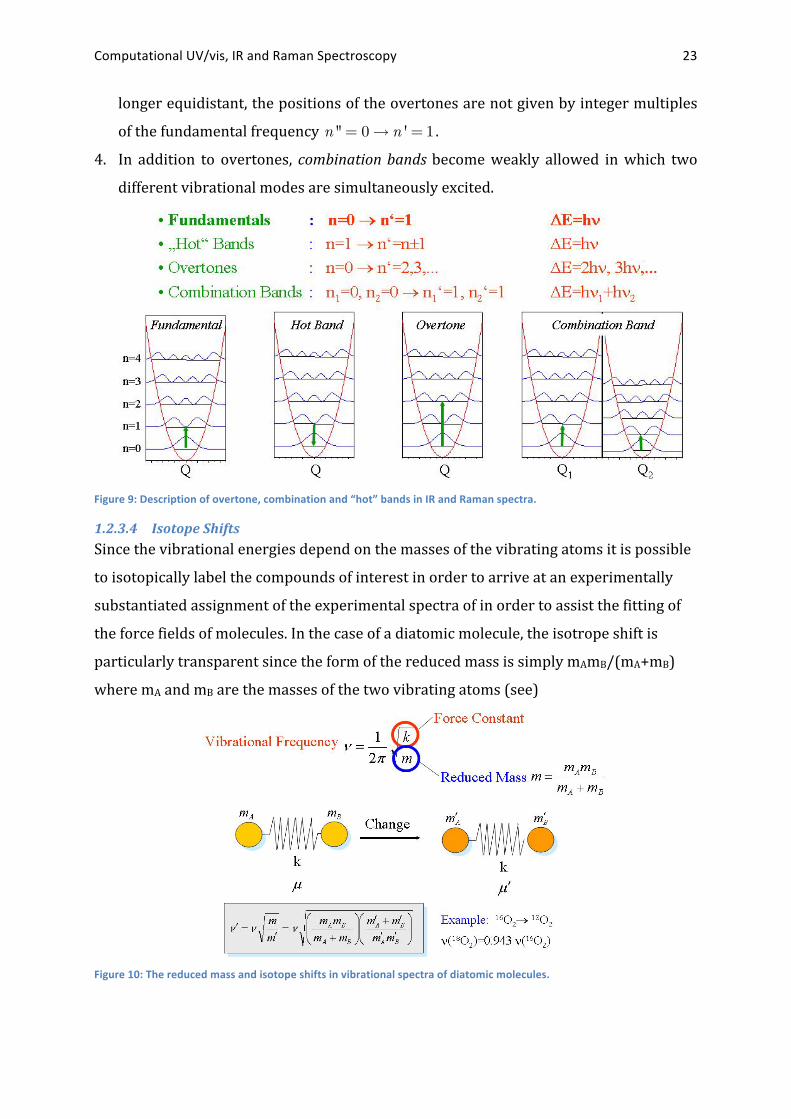
1.2.3.4 Isotope Shifts Since the vibrational energies depend on the masses of the vibrating atoms it is possible
to isotopically label the compounds of interest in order to arrive at an experimentally
substantiated assignment of the experimental spectra of in order to assist the fitting of
the force fields of molecules. In the case of a diatomic molecule, the isotrope shift is
particularly transparent since the form of the reduced mass is simply mAmB/(mA+mB)
where mA and mB are the masses of the two vibrating atoms (see)
Figure 10: The reduced mass and isotope shifts in vibrational spectra of diatomic molecules.
Computational UV/vis, IR and Raman Spectroscopy 24
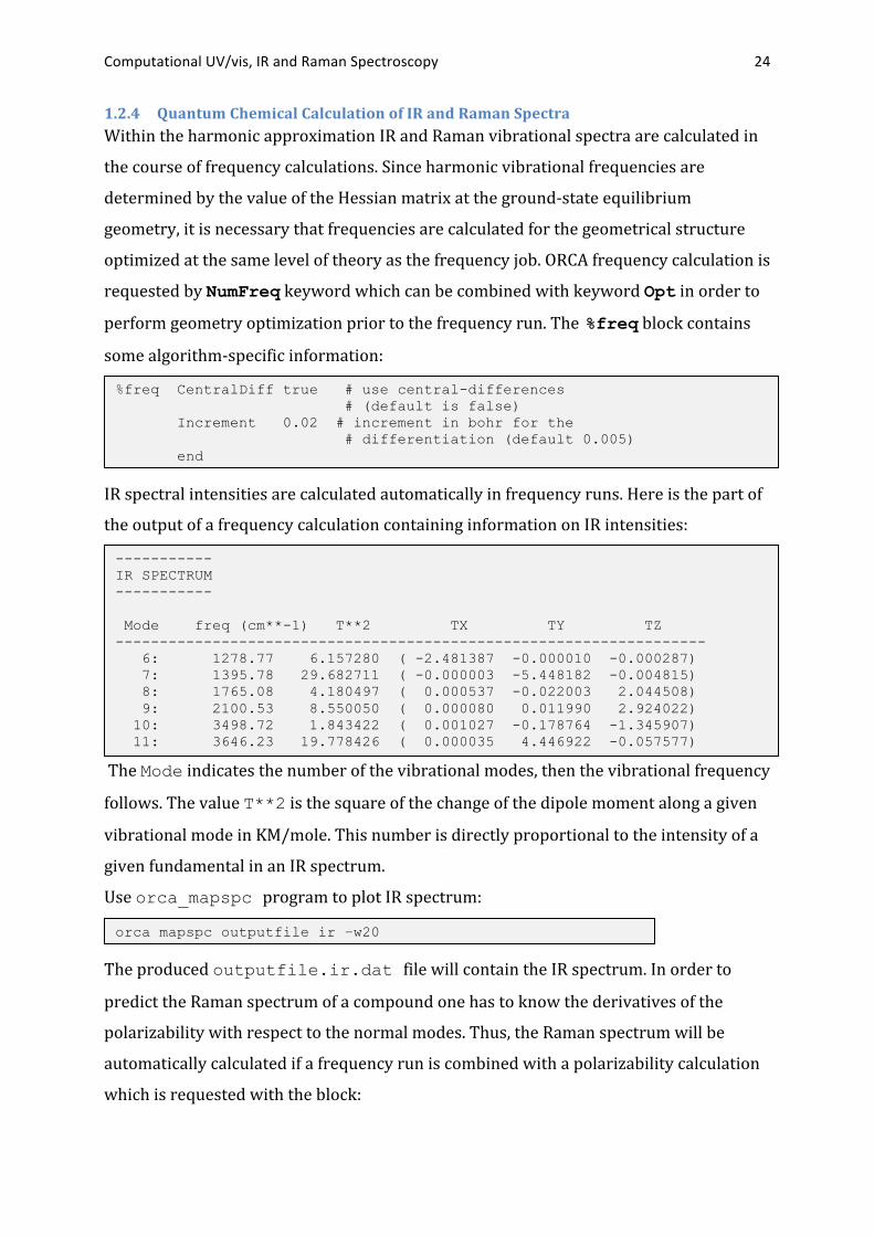
1.2.4 Quantum Chemical Calculation of IR and Raman Spectra Within the harmonic approximation IR and Raman vibrational spectra are calculated in
the course of frequency calculations. Since harmonic vibrational frequencies are
determined by the value of the Hessian matrix at the ground-‐state equilibrium
geometry, it is necessary that frequencies are calculated for the geometrical structure
optimized at the same level of theory as the frequency job. ORCA frequency calculation is
requested by NumFreq keyword which can be combined with keyword Opt in order to
perform geometry optimization prior to the frequency run. The %freq block contains
some algorithm-‐specific information:
IR spectral intensities are calculated automatically in frequency runs. Here is the part of
the output of a frequency calculation containing information on IR intensities:
The Mode indicates the number of the vibrational modes, then the vibrational frequency
follows. The value T**2 is the square of the change of the dipole moment along a given
vibrational mode in KM/mole. This number is directly proportional to the intensity of a
given fundamental in an IR spectrum.
Use orca_mapspc program to plot IR spectrum:
The produced outputfile.ir.dat file will contain the IR spectrum. In order to
predict the Raman spectrum of a compound one has to know the derivatives of the
polarizability with respect to the normal modes. Thus, the Raman spectrum will be
automatically calculated if a frequency run is combined with a polarizability calculation
which is requested with the block:
%freq CentralDiff true # use central-differences # (default is false) Increment 0.02 # increment in bohr for the # differentiation (default 0.005) end
----------- IR SPECTRUM ----------- Mode freq (cm**-1) T**2 TX TY TZ ------------------------------------------------------------------- 6: 1278.77 6.157280 ( -2.481387 -0.000010 -0.000287) 7: 1395.78 29.682711 ( -0.000003 -5.448182 -0.004815) 8: 1765.08 4.180497 ( 0.000537 -0.022003 2.044508) 9: 2100.53 8.550050 ( 0.000080 0.011990 2.924022) 10: 3498.72 1.843422 ( 0.001027 -0.178764 -1.345907) 11: 3646.23 19.778426 ( 0.000035 4.446922 -0.057577)
orca_mapspc outputfile ir –w20

Computational UV/vis, IR and Raman Spectroscopy 25
The output consists of the Raman activity (in A4/AMU) and the Raman depolarization ratios:
As with IR spectra you can get a plot of the Raman spectrum using:
The produced outputfile.raman.dat file will contain the Raman spectrum.
1.3 Description of the Experiment
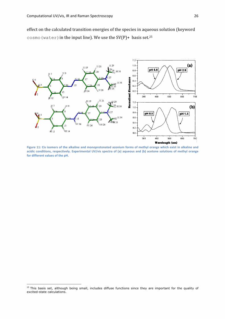
1.3.1 Calculation of UV/vis spectra. PART 1: Calculate the absorption spectra of the protonated and unprotonated forms of
the dye methyl orange (Figure 11). Since the two forms show distinct absorption
spectra, such dyes can be used as pH indicators. The protonated form (pH<3.1) is
characterized by intense absorption in the blue-‐green spectral range (450-‐550 nm),
while the absorption of the deprotonated form (pH>4.4) mainly occurs in the violet-‐blue
range (400-‐470 nm) (Figure 11).23 Consequently, upon a change of the pH from 3.1 to
4.4, methyl orange changes its color from red to yellow. In this experiment you should
try to understand this change.
We are interested in the calculation of the most intense electronic absorption band of
both, the protonated and the unprotonated form of methyl orange. Below we specify the
input files which contain geometries.24 TD-‐DFT calculations for the 10 lowest excited
states will be carried out. The COSMO approach is applied in order to model the solvent
23 Nero, J.D.; Araujo, R.E.; Gomes, A.S.L.; Melo, C.P.; (2005) J. Chem. Phys., 122, 104506.
24 Optimized with BP86/SV(P)
%elprop CalcPolar true end
-------------- RAMAN SPECTRUM -------------- Mode freq (cm**-1) Activity Depolarization -------------------------------------------------- 6: 1278.77 0.007349 0.749649 7: 1395.78 3.020010 0.749997 8: 1765.08 16.366586 0.708084 9: 2100.53 6.696490 0.075444 10: 3498.72 38.650431 0.186962 11: 3646.23 24.528483 0.748312
orca_mapspc outputfile raman –w20
Computational UV/vis, IR and Raman Spectroscopy 26
effect on the calculated transition energies of the species in aqueous solution (keyword
cosmo(water)in the input line). We use the SV(P)+ basis set.25
Figure 11: Cis isomers of the alkaline and monoprotonated azonium forms of methyl orange which exist in alkaline and acidic conditions, respectively. Experimental UV/vis spectra of (a) aqueous and (b) acetone solutions of methyl orange for different values of the pH.
25 This basis set, although being small, includes diffuse functions since they are important for the quality of excited-state calculations.
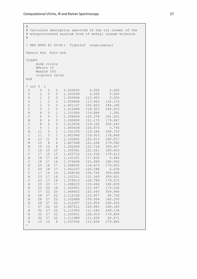
Computational UV/vis, IR and Raman Spectroscopy 27
# # Calculate absorption spectrum of the cis isomer of the # monoprotonated azonium form of methyl orange molecule # ! RKS BP86 RI SV(P)+ TightScf cosmo(water) %basis Aux Auto end %tddft mode riints NRoots 10 MaxDim 200 triplets false end * int 0 1 S 0 0 0 0.000000 0.000 0.000 O 1 0 0 1.503294 0.000 0.000 O 1 2 0 1.505496 113.903 0.000 O 1 2 3 1.504846 113.963 132.114 C 1 2 3 1.821147 105.823 246.180 C 5 1 2 1.412488 118.923 184.915 H 6 5 1 1.101906 119.884 1.391 C 6 5 1 1.396656 120.278 181.201 H 8 6 5 1.099690 121.170 179.947 C 8 6 5 1.415430 119.104 359.943 C 5 1 2 1.405438 120.673 5.790 H 11 5 1 1.101105 119.344 358.753 C 11 5 1 1.401946 119.910 178.849 H 13 11 5 1.102862 120.413 180.017 N 10 8 6 1.407048 121.294 179.582 N 15 10 8 1.292068 122.718 359.407 C 16 15 10 1.355081 121.021 180.663 C 17 16 15 1.435712 115.336 179.613 H 18 17 16 1.101331 117.832 0.440 C 18 17 16 1.379608 121.689 180.593 H 20 18 17 1.098042 118.873 179.922 C 20 18 17 1.441237 120.588 0.036 C 17 16 15 1.438195 126.765 359.889 H 23 17 16 1.102101 121.369 359.401 C 23 17 16 1.379013 120.789 179.375 H 25 23 17 1.098225 118.466 180.009 N 22 20 18 1.355001 121.367 179.530 C 27 22 20 1.466602 120.443 359.964 H 28 27 22 1.112145 110.957 60.750 H 28 27 22 1.105488 109.004 180.193 H 28 27 22 1.112207 110.954 299.654 C 27 22 20 1.467211 120.863 180.183 H 32 27 22 1.111950 111.045 299.134 H 32 27 22 1.105431 108.919 179.800 H 32 27 22 1.111988 111.009 60.471 H 15 10 8 1.037594 115.838 179.885 *
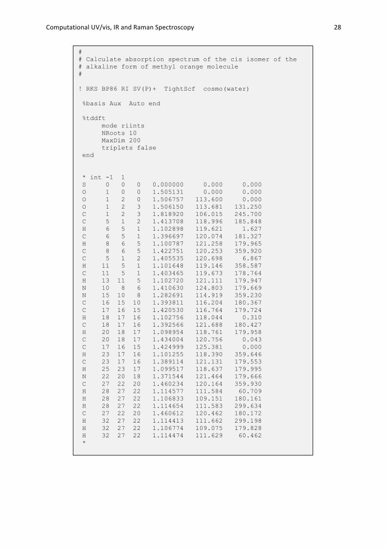
Computational UV/vis, IR and Raman Spectroscopy 28
# # Calculate absorption spectrum of the cis isomer of the # alkaline form of methyl orange molecule # ! RKS BP86 RI SV(P)+ TightScf cosmo(water) %basis Aux Auto end %tddft mode riints NRoots 10 MaxDim 200 triplets false end * int -1 1 S 0 0 0 0.000000 0.000 0.000 O 1 0 0 1.505131 0.000 0.000 O 1 2 0 1.506757 113.600 0.000 O 1 2 3 1.506150 113.681 131.250 C 1 2 3 1.818920 106.015 245.700 C 5 1 2 1.413708 118.996 185.848 H 6 5 1 1.102898 119.621 1.627 C 6 5 1 1.396697 120.074 181.327 H 8 6 5 1.100787 121.258 179.965 C 8 6 5 1.422751 120.253 359.920 C 5 1 2 1.405535 120.698 6.867 H 11 5 1 1.101648 119.146 358.587 C 11 5 1 1.403465 119.673 178.764 H 13 11 5 1.102720 121.111 179.947 N 10 8 6 1.410630 124.803 179.669 N 15 10 8 1.282691 114.919 359.230 C 16 15 10 1.393811 116.204 180.367 C 17 16 15 1.420530 116.764 179.724 H 18 17 16 1.102756 118.044 0.310 C 18 17 16 1.392566 121.688 180.427 H 20 18 17 1.098954 118.761 179.958 C 20 18 17 1.434004 120.756 0.043 C 17 16 15 1.424999 125.381 0.000 H 23 17 16 1.101255 118.390 359.646 C 23 17 16 1.389114 121.131 179.553 H 25 23 17 1.099517 118.637 179.995 N 22 20 18 1.371544 121.464 179.666 C 27 22 20 1.460234 120.164 359.930 H 28 27 22 1.114577 111.584 60.709 H 28 27 22 1.106833 109.151 180.161 H 28 27 22 1.114654 111.583 299.634 C 27 22 20 1.460612 120.462 180.172 H 32 27 22 1.114413 111.662 299.198 H 32 27 22 1.106774 109.075 179.828 H 32 27 22 1.114474 111.629 60.462 *
Computational UV/vis, IR and Raman Spectroscopy 29
• From the output, determine the most intense transitions, their excitation
energies and their oscillator strengths. Are the variations of transition energies
consistent with experimentally observed spectral changes between two forms of
methyl orange?
• Analyze the electronic structure of the two forms. Determine the nature of the
most intense transitions by inspecting the shapes of donor and acceptor MOs
with a visualization program. How do these orbitals change upon going from
unprotonated to protonated species?
• Use the orca_mapspc program to plot absorption spectra in the visible spectral
range and compare them with the experimental spectra.
PART 2: Calculate the vibrational structure of the absorption band and resonance
Raman spectra corresponding to the electronic transition 11Ag →11Bu of trans-‐1,3,5-‐
hexatrien. Assuming the IHMDO model, the calculation of vibronic structure in
absorption spectra26 for dipole-‐allowed transitions involves two stages. First one
should calculate the transition energy, transition dipole moment and origin
displacement of the excited state relative to the ground state along totally symmetric
normal modes. On the second stage the calculated parameters are employed in order
to simulate the absorption spectrum in a user-‐specified spectral range. Within the
harmonic approximation, the origin displacements along different normal modes
may be approximated by means of excited-‐state energy-‐gradient calculations. This
type of job is specified below in the ORCA input. We have used the geometry of
hexatriene optimized at the RHF/SV(P) level. The program employs the Hessian
matrix obtained from a corresponding frequency calculation since it provides
frequencies and normal modes which are used in the transformation of the energy
gradient from Cartesian to normal coordinates. Thus, the name of the Hessian file is
specified in the %rr block via the keyword HessName.
26 as well as resonance Raman spectra; however, the resonance Raman technique will not be covered here.

Computational UV/vis, IR and Raman Spectroscopy 30
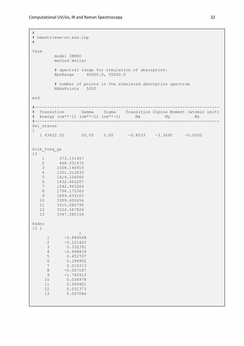
At the end of the ORCA run you get the file hexatriene-uv.asa.inp which provides
the input information for spectral simulation. The simulation part is performed in the
framework of Heller time-‐dependent theory implemented in stand-‐alone program
orca_asa.27 The basic structure of the file is shown below. In the input you will need to
modify the parameters concerning various details of the simulation like spectral range
and number of points for absorption. The input file for spectral simulation also contains
27 The theory is explained in Petrenko, T.; Neese, F. (2007) Analysis and Prediction of Absorption Bandshapes, Fluorescence Bandshapes, Resonance Raman Intensities and Excitation Profiles using the Time Dependent Theory of Electronic Spectroscopy. J. Chem. Phys., 127, 164319; Neese, F.; Petrenko, T.; Ganyushin, D.; Olbrich, G. (2007) Advanced Aspects of ab initio Theoretical Spectroscopy of Open-Shell Transition Metal Ions. Coord. Chem. Rev., 205, 288-327
# hexatriene-uv.inp # # CIS Normal Mode Gradient Calculation # ! RHF TightSCF SV(P) Grid4 NoFinalGrid NMGrad %cis NRoots 1 EWin -10000, 10000 MaxDim 200 ETol 1e-7 RTol 1e-7 triplets false end %rr HessName= "hexatriene.hess" states 1 # perform energy-gradient calculation for the 1st #excited state Tdnc 0.005 # threshold for dimensionless displacement to be # included in the input file for spectra simulations # generated at the end of the program run ASAInput true # generate the input file for spectral simulations end * xyz 0 1 C -0.007965 0.666889 -0.000000 H -0.961692 1.187002 -0.000000 C 1.194639 1.503680 0.000000 H 2.146084 0.980277 0.000000 C 1.184814 2.831999 -0.000000 H 0.257404 3.396037 -0.000000 H 2.105024 3.404491 0.000000 C 0.007965 -0.666889 -0.000000 H 0.961692 -1.187002 -0.000000 C -1.194639 -1.503680 0.000000 H -2.146084 -0.980277 0.000000 C -1.184814 -2.831999 -0.000000 H -0.257404 -3.396037 -0.000000 H -2.105024 -3.404491 0.000000 *

Computational UV/vis, IR and Raman Spectroscopy 31
the following blocks specifying the paramteres for the IMDHO model which were
calculated upon ORCA run:
• %el_states block specifies information about each electronic state including
adiabatic minima transition energy, electronic transition dipole moment
components, homogeneous linewidth parameter (Gamma), standard deviation of
transition energy (Sigma, also called inhomogeneous linewidth parameter).
• %vib_freq_gs block contains ground-‐state vibrational frequencies of
vibronically active modes.
• %sdnc block specifies dimensionless normal coordinate displacements for
vibronically active modes.
Computational UV/vis, IR and Raman Spectroscopy 32
# # hexatriene-uv.asa.inp # %sim model IMDHO method Heller # spectral range for simulation of absorption: AbsRange 40000.0, 55000.0 # number of points in the simulated absorption spectrum NAbsPoints 5000 end #--------------------------------------------------------------------------- # Transition Gamma Sigma Transition Dipole Moment (atomic unit) # Energy (cm**-1) (cm**-1) (cm**-1) Mx My Mz #--------------------------------------------------------------------------- $el_states 1 1 43422.32 50.00 0.00 -0.8533 -3.3690 -0.0000 $vib_freq_gs 13 1 373.151457 2 468.331475 3 1008.146916 4 1301.212433 5 1414.106060 6 1432.662207 7 1542.963264 8 1796.175363 9 1899.633103 10 3309.402656 11 3315.060790 12 3324.587826 13 3397.380154 $sdnc 13 1 1 1 -0.689568 2 -0.121420 3 0.332391 4 -0.998839 5 0.452707 6 0.186902 7 0.210313 8 -0.007187 9 -1.782913 10 0.034978 11 0.069401 12 0.031373 13 0.007086
Computational UV/vis, IR and Raman Spectroscopy 33
At the end of the program run you will get the file hexatriene-uv.abs.dat
containing the absoption spectrum.
Now:
• Plot the spectrum. Determine the position of the 0-‐0 vibronic peak in the
absorption. Locate the vibronic peak with the maximum intensity and compare it
with the calculated vertical transition energy. Explain the difference.
• Identify the most important overtone and combination transitions in the
absorption band. How do their intensities correlate with the values of
dimensionless normal coordinate displacements given in the input?
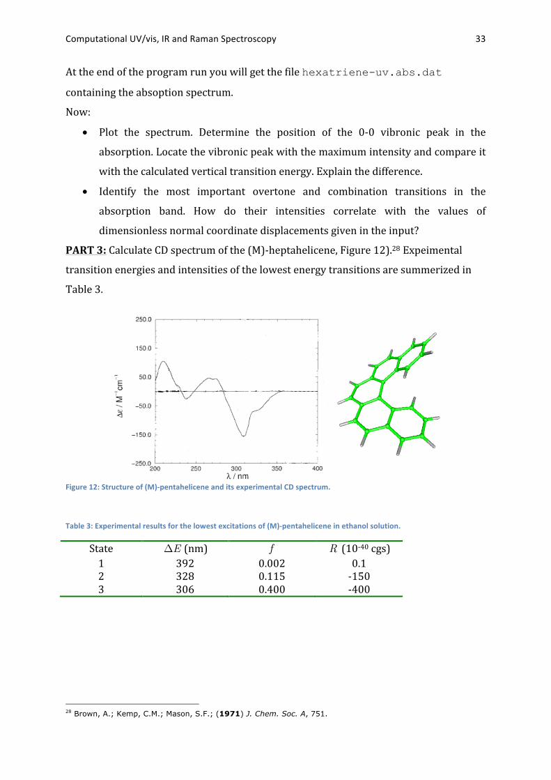
PART 3: Calculate CD spectrum of the (M)-‐heptahelicene, Figure 12).28 Expeimental
transition energies and intensities of the lowest energy transitions are summerized in
Table 3.
Figure 12: Structure of (M)-‐pentahelicene and its experimental CD spectrum.
Table 3: Experimental results for the lowest excitations of (M)-‐pentahelicene in ethanol solution.
State !E (nm) f R (10-‐40 cgs) 1 392 0.002 0.1 2 328 0.115 -‐150 3 306 0.400 -‐400
28 Brown, A.; Kemp, C.M.; Mason, S.F.; (1971) J. Chem. Soc. A, 751.
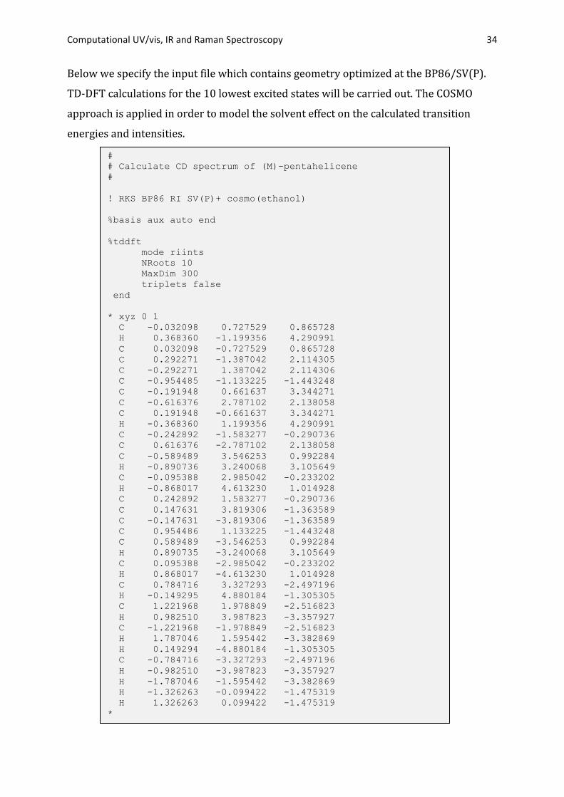
Computational UV/vis, IR and Raman Spectroscopy 34
Below we specify the input file which contains geometry optimized at the BP86/SV(P).
TD-‐DFT calculations for the 10 lowest excited states will be carried out. The COSMO
approach is applied in order to model the solvent effect on the calculated transition
energies and intensities.
# # Calculate CD spectrum of (M)-pentahelicene # ! RKS BP86 RI SV(P)+ cosmo(ethanol) %basis aux auto end %tddft mode riints NRoots 10 MaxDim 300 triplets false end * xyz 0 1 C -0.032098 0.727529 0.865728 H 0.368360 -1.199356 4.290991 C 0.032098 -0.727529 0.865728 C 0.292271 -1.387042 2.114305 C -0.292271 1.387042 2.114306 C -0.954485 -1.133225 -1.443248 C -0.191948 0.661637 3.344271 C -0.616376 2.787102 2.138058 C 0.191948 -0.661637 3.344271 H -0.368360 1.199356 4.290991 C -0.242892 -1.583277 -0.290736 C 0.616376 -2.787102 2.138058 C -0.589489 3.546253 0.992284 H -0.890736 3.240068 3.105649 C -0.095388 2.985042 -0.233202 H -0.868017 4.613230 1.014928 C 0.242892 1.583277 -0.290736 C 0.147631 3.819306 -1.363589 C -0.147631 -3.819306 -1.363589 C 0.954486 1.133225 -1.443248 C 0.589489 -3.546253 0.992284 H 0.890735 -3.240068 3.105649 C 0.095388 -2.985042 -0.233202 H 0.868017 -4.613230 1.014928 C 0.784716 3.327293 -2.497196 H -0.149295 4.880184 -1.305305 C 1.221968 1.978849 -2.516823 H 0.982510 3.987823 -3.357927 C -1.221968 -1.978849 -2.516823 H 1.787046 1.595442 -3.382869 H 0.149294 -4.880184 -1.305305 C -0.784716 -3.327293 -2.497196 H -0.982510 -3.987823 -3.357927 H -1.787046 -1.595442 -3.382869 H -1.326263 -0.099422 -1.475319 H 1.326263 0.099422 -1.475319 *
Computational UV/vis, IR and Raman Spectroscopy 35
Now: • From the output, determine the most intense transitions, their excitation
energies, oscillator strengths, and rotatory strengths. Perform the assignement of
the experimentally observed optical transitions. 29
• Determine the nature of the most intense transitions by inspecting the shapes of
donor and acceptor MOs with a visualization program.
• Use the orca_mapspc program to plot CD spectrum in appropriate spectral
range and compare it with the experimental spectrum.
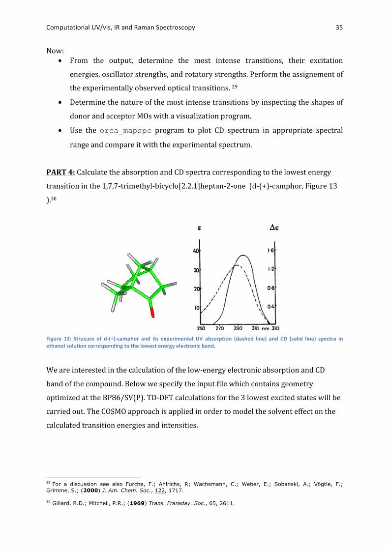
PART 4: Calculate the absorption and CD spectra corresponding to the lowest energy
transition in the 1,7,7-‐trimethyl-‐bicyclo[2.2.1]heptan-‐2-‐one (d-‐(+)-‐camphor, Figure 13
).30
Figure 13: Strucure of d-‐(+)-‐camphor and its experimental UV absorption (dashed line) and CD (solid line) spectra in ethanol solution corresponding to the lowest energy electronic band.
We are interested in the calculation of the low-‐energy electronic absorption and CD
band of the compound. Below we specify the input file which contains geometry
optimized at the BP86/SV(P). TD-‐DFT calculations for the 3 lowest excited states will be
carried out. The COSMO approach is applied in order to model the solvent effect on the
calculated transition energies and intensities.
29 For a discussion see also Furche, F.; Ahlrichs, R; Wachsmann, C.; Weber, E.; Sobanski, A.; Vögtle, F.; Grimme, S.; (2000) J. Am. Chem. Soc., 122, 1717.
30 Gillard, R.D.; Mitchell, P.R.; (1969) Trans. Fraraday. Soc., 65, 2611.
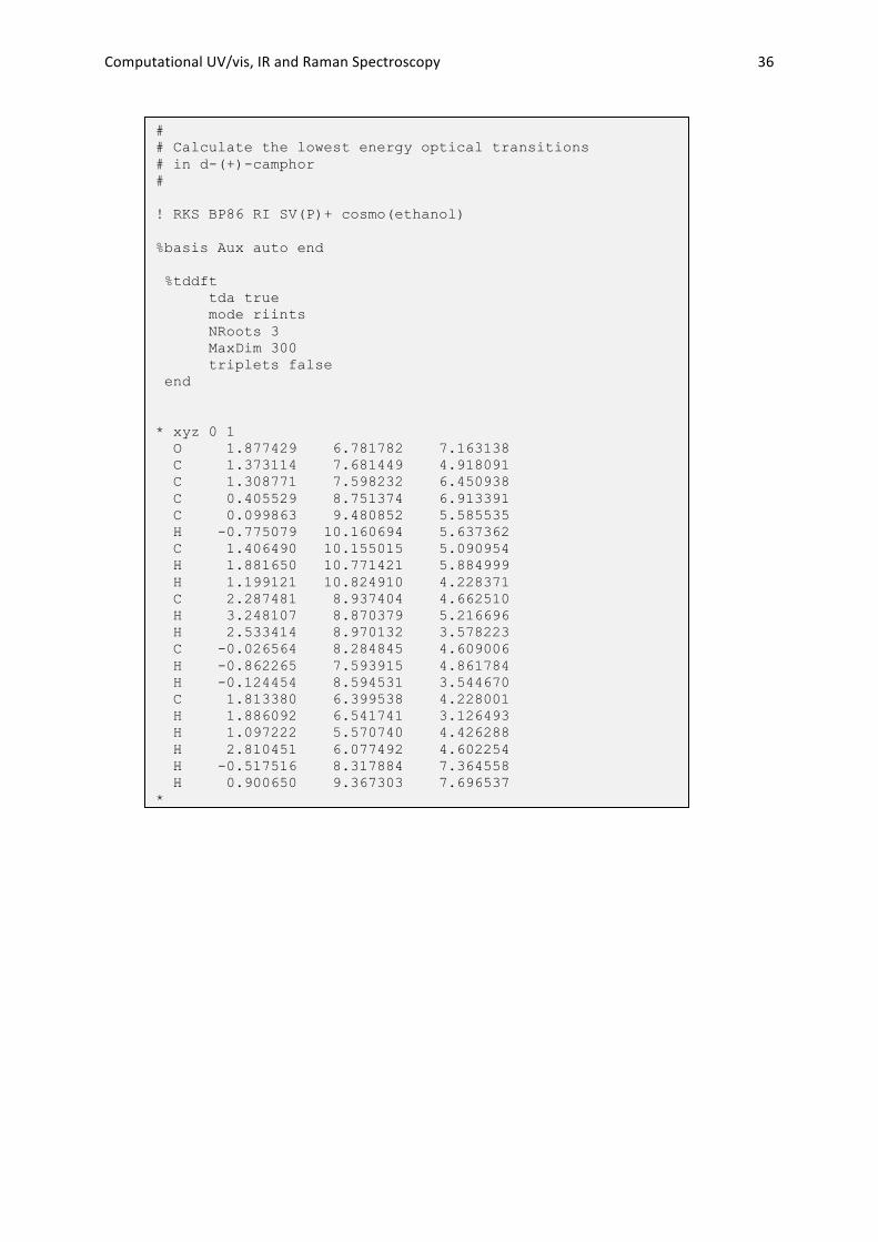
Computational UV/vis, IR and Raman Spectroscopy 36
# # Calculate the lowest energy optical transitions # in d-(+)-camphor # ! RKS BP86 RI SV(P)+ cosmo(ethanol) %basis Aux auto end %tddft tda true mode riints NRoots 3 MaxDim 300 triplets false end * xyz 0 1 O 1.877429 6.781782 7.163138 C 1.373114 7.681449 4.918091 C 1.308771 7.598232 6.450938 C 0.405529 8.751374 6.913391 C 0.099863 9.480852 5.585535 H -0.775079 10.160694 5.637362 C 1.406490 10.155015 5.090954 H 1.881650 10.771421 5.884999 H 1.199121 10.824910 4.228371 C 2.287481 8.937404 4.662510 H 3.248107 8.870379 5.216696 H 2.533414 8.970132 3.578223 C -0.026564 8.284845 4.609006 H -0.862265 7.593915 4.861784 H -0.124454 8.594531 3.544670 C 1.813380 6.399538 4.228001 H 1.886092 6.541741 3.126493 H 1.097222 5.570740 4.426288 H 2.810451 6.077492 4.602254 H -0.517516 8.317884 7.364558 H 0.900650 9.367303 7.696537 *
Computational UV/vis, IR and Raman Spectroscopy 37
Now:
• From the output, determine the transitions, which energy most closely matches
the experimental one. Determine the nature of the transition by inspecting the
shapes of donor and acceptor MOs with a visualization program.
• Use the orca_mapspc program to plot absorption and CD spectra in the spectral
range around 300 nm using appropriate value of the bandwidth which roughly
matches the experimental one. Compare experimental and theoretical plots.
• Does the rotatory strength have the proper sign for the given transitions? What
parameter, that can be rather sensitive to the level of calculation, can result in
observed disagreement? As a hint, consider the the scalar product of the
transition electric dipole and magnetic dipole moments in the form
D0!I"M
0!I= D
0!IM
0!Icos! .
1.3.2 Calculation of IR and Raman spectra PART 1: Optimize the geometries, calculate vibrational frequencies, IR and Raman
intensities of the following diatomic molecules using the BP86 functional and the TZVP
basis set:
• CO : ωexp= 2170 cm-‐1 • HF : ωexp= 4138 cm-‐1 • ClF : ωexp= 786 cm-‐1 • N2 : ωexp= 2359 cm-‐1 • HCl : ωexp= 2991 cm-‐1 • Cl2 : ωexp= 560 cm-‐1 Now: • Analyze the origin of the trends in the calculated IR intensities using population
analysis and chemical intuition
• Why do the stretching vibrations of the homonuclear diatomics do not show any
IR intensity? Provide a qualitative explanation on the origin of IR intensity for the
heteronuclear species.
• Compare the calculated harmonic frequencies with the experimental harmonic
frequencies. How reliable are the DFT results?31
31 In general, the calculations always produce harmonic force constants and therefore also harmonic frequencies. The underlying assumption is that the potential energy surfaces behave exactly quadratically. In reality, however, the potentials are anharmonic and this leads to important alternations in the spacing of the vibrational levels. Some of these aspects will be studied for diatomic molecules in section Error! Reference source not found. on page 166. However, experimental harmonic frequencies are only known for very small molecules and anharmonic frequencies are difficult to calculate. In practice, this limits the accuracy of the

Computational UV/vis, IR and Raman Spectroscopy 38
PART 2: Optimize the geometry, calculate vibrational frequencies, IR and Raman
intensities of the benzene molecule using the BP86 functional and the TZVP basis set.
Experimental vibrational frequencies of the benzene are known from IR and Raman
measurements:
• IR : 1485 cm-‐1 • Raman : 605.0, 991.6, 1178.0, 1595.0 cm-‐1
Here is the input file for ORCA calculation:
Now: • Assign experimental vibrational frequencies. Determine the character of IR and
Raman active vibrations using the gOpenMol program for visualization.
• Plot the experimental versus the calculated frequencies.
• Calculate the parameters of a linear regression analysis. How reliable are your
predictions of vibrational frequencies? What is your mean deviation from
experiment, what is your maximum deviation?
• The benzene molecule possesses a center of inversion. Show complementary
nature of Raman and IR spectra on the basis of the calculated IR intensities and
comparison between theory and experiment and one usually compares calculated harmonic frequencies with observed fundamentals (which contain anharmonic contributions).
! RKS BP86 RI TZVP TZV/J TightOpt TightScf Grid4 NoFinalGrid NumFreq %freq CentralDiff true Increment 0.02 end %elprop Polar true end # vibrational analysis of benzene molecule * xyz 0 1 C 0.000000 -0.7000000000 1.2124355653 H 0.000000 -1.2500000000 2.1650635095 C 0.000000 -1.4000000000 0.0000000000 H 0.000000 -2.5000000000 0.0000000000 C 0.000000 -0.7000000000 -1.2124355653 H 0.000000 -1.2500000000 -2.1650635095 C 0.000000 0.7000000000 1.2124355653 H 0.000000 1.2500000000 2.1650635095 C 0.000000 1.4000000000 0.0000000000 H 0.000000 2.5000000000 0.0000000000 C 0.000000 0.7000000000 -1.2124355653 H 0.000000 1.2500000000 -2.1650635095 *

Computational UV/vis, IR and Raman Spectroscopy 39
Raman activities. Which symmetry species are active in IR and which in Raman?
Which vibrations are forbidden in both IR and Raman spectra?
PART 3: Optimize the geometries and calculate vibrational frequencies of the following
molecules using the BP86 functional and the TZVP basis set:
• C2H2 • C2H4 • C2H6 JOB:
• Discuss the trend in the variation of frequency of CC stretching mode between the
molecules. How do the frequencies depend on the bond order? Compare the
results with the characteristic frequencies known for C–C, C=C and C≡C bonds.
• Use the orca_vib program to obtain estimates of the C-‐C stretching force
constants. How do they vary with bond order?
• Provide a qualitative explanation of the observed trend on the basis of chemical
intuition.
PART 4: Optimize the geometry, calculate vibrational frequencies, IR and Raman
intensities of the glycine molecule (H2N-‐CH2-‐COOH) using the BP86 functional and the
TZVP basis set.
The input file is specified below:
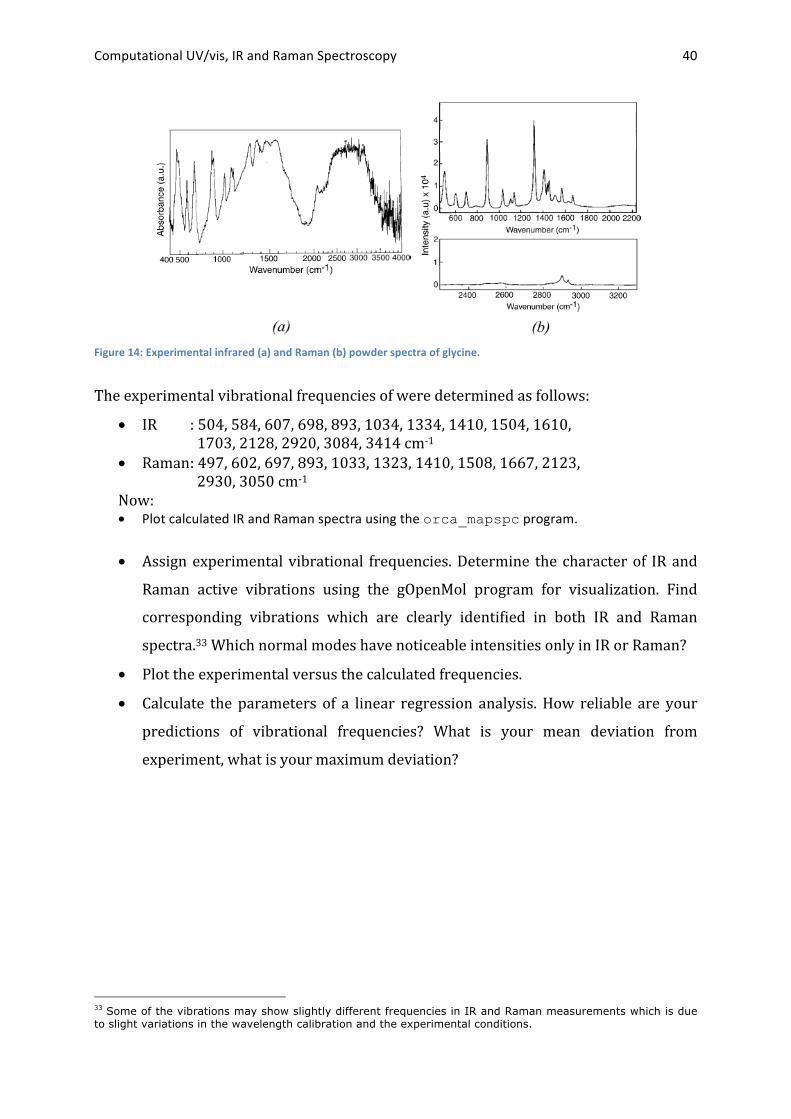
The experimental IR and Raman powder spectra of glycine32 are given in Figure 14.
32 Kumar, S.; Rai, A.K.; Singh, V.B.; Rai, S.B.; (2005) Spectrochim. Acta Part A, 61, 2741-2746.
! RKS BP86 RI TZVP TZV/J TightOpt TightScf Grid4 NoFinalGrid NumFreq %freq CentralDiff true Increment 0.02 end %elprop Polar true end * xyz 0 1 N 0.417502 -1.939309 0.000000 C -0.563503 -0.866622 0.000000 C 0.000000 0.555853 0.000000 H 1.029096 -1.853448 0.815576 H 1.029096 -1.853448 -0.815576 H -1.225791 -0.963395 -0.876292 H -1.225791 -0.963395 0.876292 O 1.179353 0.850856 0.000000 O -1.002263 1.487634 0.000000 H -0.564825 2.365543 0.000000 *
Computational UV/vis, IR and Raman Spectroscopy 40
Figure 14: Experimental infrared (a) and Raman (b) powder spectra of glycine.
The experimental vibrational frequencies of were determined as follows:
• IR : 504, 584, 607, 698, 893, 1034, 1334, 1410, 1504, 1610, 1703, 2128, 2920, 3084, 3414 cm-‐1
• Raman : 497, 602, 697, 893, 1033, 1323, 1410, 1508, 1667, 2123, 2930, 3050 cm-‐1
Now: • Plot calculated IR and Raman spectra using the orca_mapspc program.
• Assign experimental vibrational frequencies. Determine the character of IR and
Raman active vibrations using the gOpenMol program for visualization. Find
corresponding vibrations which are clearly identified in both IR and Raman
spectra.33 Which normal modes have noticeable intensities only in IR or Raman?
• Plot the experimental versus the calculated frequencies.
• Calculate the parameters of a linear regression analysis. How reliable are your
predictions of vibrational frequencies? What is your mean deviation from
experiment, what is your maximum deviation?
33 Some of the vibrations may show slightly different frequencies in IR and Raman measurements which is due to slight variations in the wavelength calibration and the experimental conditions.

Computational UV/vis, IR and Raman Spectroscopy 41