Embed Size (px)
Citation preview

1. Data summary and visualization
1

Summary statistics
1 # The UScereal data frame has 65 rows and 11 columns.2 # The data come from the 1993 ASA Statistical Graphics Exposition,3 # and are taken from the mandatory F&DA food label.4 # The data have been normalized here to a portion of one American cup.5 >library(MASS)6 >data(UScereal)7 >summary(UScereal)
1 mfr calories protein fat sodium2 G:22 Min. : 50.0 Min. : 0.7519 Min. :0.000 Min. : 0.03 K:21 1st Qu.:110.0 1st Qu.: 2.0000 1st Qu.:0.000 1st Qu.:180.04 N: 3 Median :134.3 Median : 3.0000 Median :1.000 Median :232.05 P: 9 Mean :149.4 Mean : 3.6837 Mean :1.423 Mean :237.86 Q: 5 3rd Qu.:179.1 3rd Qu.: 4.4776 3rd Qu.:2.000 3rd Qu.:290.07 R: 5 Max. :440.0 Max. :12.1212 Max. :9.091 Max. :787.98 fibre carbo sugars shelf9 Min. : 0.000 Min. :10.53 Min. : 0.00 Min. :1.000
10 1st Qu.: 0.000 1st Qu.:15.00 1st Qu.: 4.00 1st Qu.:1.00011 Median : 2.000 Median :18.67 Median :12.00 Median :2.00012 Mean : 3.871 Mean :19.97 Mean :10.05 Mean :2.16913 3rd Qu.: 4.478 3rd Qu.:22.39 3rd Qu.:14.00 3rd Qu.:3.00014 Max. :30.303 Max. :68.00 Max. :20.90 Max. :3.00015
16 potassium vitamins17 Min. : 15.0 100% : 5
2

18 1st Qu.: 45.0 enriched:5719 Median : 96.6 none : 320 Mean :159.121 3rd Qu.:220.022 Max. :969.7
1 ># correlation matrix between some variables2 >cor(UScereal[c("calories","protein","fat","fibre","sugars")])
1 calories protein fat fibre sugars2 calories 1.0000000 0.7060105 0.5901757 0.3882179 0.49529423 protein 0.7060105 1.0000000 0.4112661 0.8096397 0.18484844 fat 0.5901757 0.4112661 1.0000000 0.2260715 0.41567405 fibre 0.3882179 0.8096397 0.2260715 1.0000000 0.14891586 sugars 0.4952942 0.1848484 0.4156740 0.1489158 1.0000000
>library(MASS)
>data(UScereal)
>summary(UScereal) # summary statiscs for each variable
mfr calories protein fat sodiumG:22 Min. : 50.0 Min. : 0.7519 Min. :0.000 Min. : 50.0K:21 1st Qu.:110.0 1st Qu.: 2.0000 1st Qu.:0.000 1st Qu.:180.0N: 3 Median :134.3 Median : 3.0000 Median :1.000 Median :232.0P: 9 Mean :149.4 Mean : 3.6837 Mean :1.423 Mean :237.8Q: 5 3rd Qu.:179.1 3rd Qu.: 4.4776 3rd Qu.:2.000 3rd Qu.:290.0R: 5 Max. :440.0 Max. :12.1212 Max. :9.091 Max. :787.9
3

fibre carbo sugars shelfMin. : 0.000 Min. :10.53 Min. : 0.00 Min. :1.0001st Qu.: 0.000 1st Qu.:15.00 1st Qu.: 4.00 1st Qu.:1.000Median : 2.000 Median :18.67 Median :12.00 Median :2.000Mean : 3.871 Mean :19.97 Mean :10.05 Mean :2.1693rd Qu.: 4.478 3rd Qu.:22.39 3rd Qu.:14.00 3rd Qu.:3.000Max. :30.303 Max. :68.00 Max. :20.90 Max. :3.000
potassium vitaminsMin. : 15.0 100% : 51st Qu.: 45.0 enriched:57Median : 96.6 none : 3Mean :159.13rd Qu.:220.0Max. :969.7
># correlation matrix between some variables
>cor(UScereal[c("calories","protein","fat","fibre","sugars")])
calories protein fat fibre sugarscalories 1.0000000 0.7060105 0.5901757 0.3882179 0.4952942protein 0.7060105 1.0000000 0.4112661 0.8096397 0.1848484
fat 0.5901757 0.4112661 1.0000000 0.2260715 0.4156740fibre 0.3882179 0.8096397 0.2260715 1.0000000 0.1489158
sugars 0.4952942 0.1848484 0.4156740 0.1489158 1.0000000
4

1. Density visualization
Histogram
>hist(UScereal[,"protein"], main="UScereal data", xlab="protein")
UScereal data
protein
Freq
uenc
y
0 2 4 6 8 10 12 14
05
1015
20
5

2. Density visualization
Kernel smoothing
>plot(density(UScereal[,"protein"],kernel="gaussian"), main="UScereal data",
+ xlab="protein")
0 5 10
0.00
0.05
0.10
0.15
0.20
UScereal data
protein
Dens
ity
6

Boxplot
>mfr=UScereal["mfr"]
>boxplot(UScereal[mfr=="K","protein"], UScereal[mfr=="G", "protein"],
+ names=c("Kellogs", "General Mills"), xlab="Manufacturer", ylab="protein"))
Kellogs General Mills
24
68
1012
Manufacturer
prot
ein
7

Quantile plot
QQ plot displays (zk/(n+1), x(k)), zq is qth quantile of N (0, 1) Φ(zq) = q,
0 < q < 1.
>qqnorm(UScereal$calories)
−2 −1 0 1 2
100
200
300
400
Normal Q−Q Plot
Theoretical Quantiles
Samp
le Qu
antile
s
8

Relations between two variables
Scatterplot
>plot(UScereal$fat, UScereal$calories, xlab="Fat", ylab="Calories")
0 2 4 6 8
100
200
300
400
Fat
Calor
ies
9

Relations between more than two variables
Scatterplot matrix
>plot(UScereal[c("calories", "fat", "protein", "sugars","fibre", "sodium")])
calories
0 2 4 6 8 0 5 10 15 20 0 200 600
100
200
300
400
02
46
8
fat
protein
24
68
1012
05
1015
20
sugars
fibre
05
1015
2025
30
100 300
020
040
060
080
0
2 4 6 8 12 0 10 20 30
sodium
10

Parallel plot
>parallel( UScereal[, c("calories","protein", "fat", "fibre")])
Min Max
calories
protein
fat
fibre
11

2. Association rules
(Market basket analysis)
12
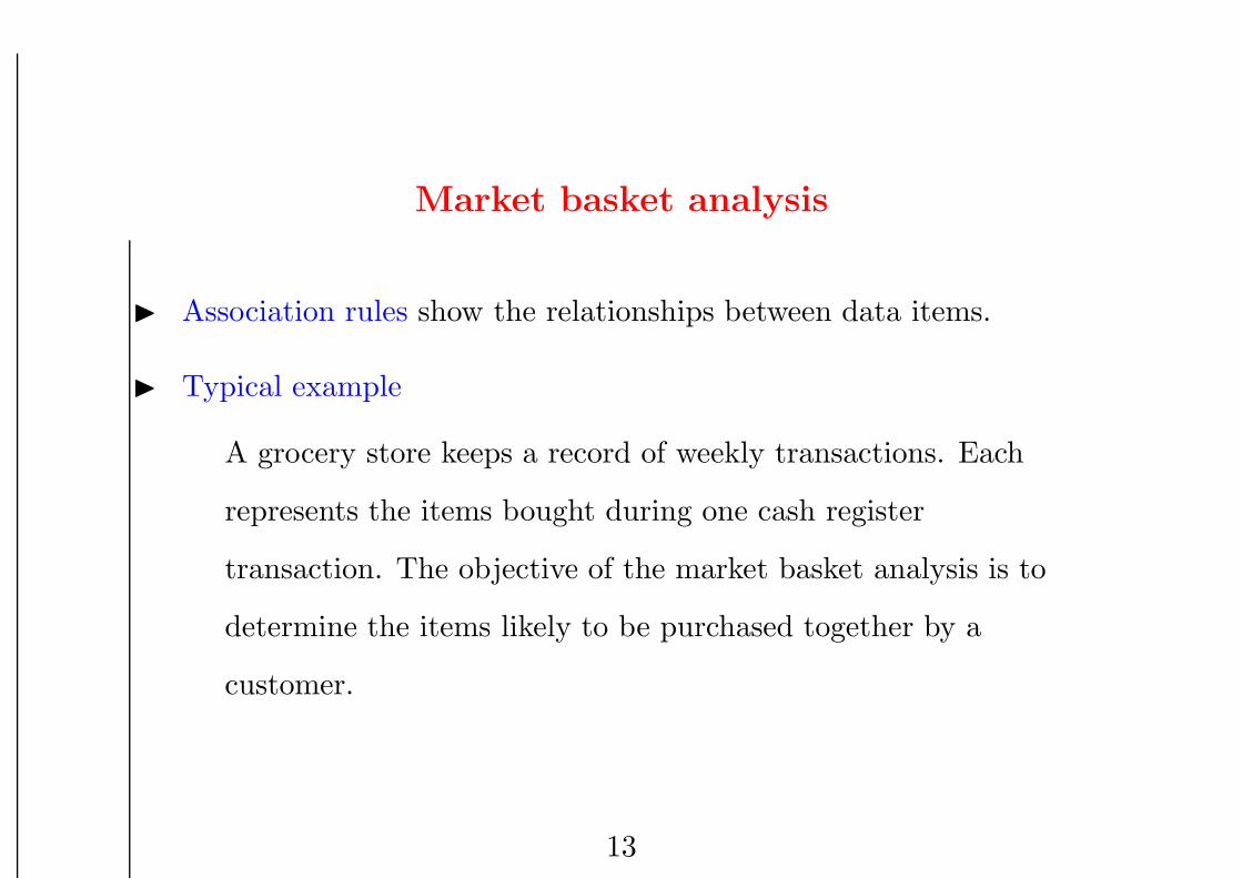
Market basket analysis
◮ Association rules show the relationships between data items.
◮ Typical example
A grocery store keeps a record of weekly transactions. Each
represents the items bought during one cash register
transaction. The objective of the market basket analysis is to
determine the items likely to be purchased together by a
customer.
13

Example
◮ Items: {Beer, Bread, Jelly, Milk, PeanutButter}
Transaction Items
t1 Bread, Jelly, PeanutButter
t2 Bread, PeanutButter
t3 Bread, Milk, PeanutButter
t4 Beer, Bread
t5 Beer, Milk
◮ 100% of the time that PeanutButter is purchased, so is Bread.
◮ 33.3% of the time PeanutButter is purchased, Jelly is also
purchased.
◮ PeanutButter exists in 60% of the overall transactions.
14

Definitions
◮ Given:
� a set of items I = {I1, . . . , Im}
� a database of transactions D = {t1, . . . , tn} where ti = {Ii1 , . . . , Iik}
and Iij ∈ I
◮ Association rule
Let X and Y be two disjoint subsets (itemsets) of I . We say that
Y is associated with X (and write X ⇒ Y ) if the appearance of
X in an transaction ”usually” implies that Y occur in that
transaction too. We identify
X ⇔ {X is purchased}
15

Support and confidence
◮ Support s of an association rule X ⇒ Y is the percentage of
transactions in the database that contain X ∩ Y
s(X ⇒ Y ) = P (X ∩ Y ) =1
n
n∑
i=1
1
{
ti ⊇ (X ∩ Y )}
.
◮ Confidence or strength α of an association rule X ⇒ Y is the ratio of
the number of transactions that contain X ∩ Y to the number of
transactions that contain X
α(X ⇒ Y ) = P (Y |X) =P (X ∩ Y )
P (X)=
∑ni=1 1
{
ti ⊇ (X ∩ Y )}
∑ni=1 1
{
ti ⊇ X}
◮ Problem: identify all rules with support and confidence ≥ s0 and α0.
16

Support and confidence of some rules
X ⇒ Y s α
Bread ⇒ PeanutButter 60% 75%
PeanutButter ⇒ Bread 60% 100%
Beer ⇒ Bread 20% 50%
PeanutButter ⇒ Jelly 20% 33.3%
Jelly ⇒ PeanutButter 20% 100%
Jelly ⇒ Milk 0% 0%
17

Other measures of rules quality
Rules with high support and confidence may be obvious (not interesting).
◮ Lift (interest)
lift(X ⇒ Y ) =P (X ∩ Y )
P (X)P (Y )=
1n
∑ni=1 1(ti ⊇ X ∩ Y )
1n
∑ni=1 1(ti ⊇ X) 1n
∑ni=1 1(ti ⊇ Y )
Rules with lift ≥ 1 are interesting.
◮ Conviction
conviction(X ⇒ Y ) =P (X)P (Y c)
P (X ∩ Y c)
=1n
∑ni=1 1{ti ⊇ X} 1
n
∑ni=1 1{ti ⊇ Y c}
1n
∑ni=1 1{ti ⊇ X ∩ Y c}
conviction = 1 if X and Y are not related. Rules that always hold
have conviction = ∞.
18

Lift and conviction of some rules
X ⇒ Y Lift Conviction
Bread ⇒ PeanutButter 54
85
PeanutButter ⇒ Bread 54 ∞
Beer ⇒ Bread 58
25
PeanutButter ⇒ Jelly 53
65
Jelly ⇒ PeanutButter 53 ∞
Jelly ⇒ Milk 0 35
19

Mining rules from frequent itemsets
1. Find frequent itemsets (itemset whose number of occurrences is above
a threshold s).
2. Generate rules from frequent itemsets.
Input: D - database, I - collection of all items,
L-collection of all frequent itemsets, s0, α0.
Output: R - association rules satisfying s0 and α0.
R = ∅;
for each ℓ ∈ L do
for each x ⊂ ℓ such that x 6= ∅ do
ifsupport(ℓ)support(x) ≥ α then R = R ∪ {x ⇒ (ℓ− x)};
20

Example
Assume s0 = 30% and α0 = 50%.
◮ Frequent itemset L
{{Beer},{Bread},{Milk},{PeanutButter},{Bread,PeanutButter}}
◮ For ℓ = {Bread, PeanutButter} we have two subsets:
support({Bread, PeanutButter})
support({Bread})=
60
80= 0.75 > 0.5
support({Bread, PeanutButter})
support({PeanutButter})=
60
60= 1 > 0.5
◮ Conclusion:
PeanutButter ⇒ Bread and Bread ⇒ PeanutButter are valid
association rules.
21

Finding frequent itemsets: apriori algorithm
◮ Frequent itemset property
Any subset of frequent itemset must be frequent
◮ Basic idea:
– Look at candidate sets of size i
– Choose frequent itemsets of the size i
– Generate frequent itemsets of size i+ 1 by joining (taking unions
of) frequent itemsets found till pass i+ 1.
22

Example: apriori algorithm
s0 = 30%, α0 = 50%
Pass Candidates Frequent itemsets
1 {Beer},{Bread},{Jelly} {Beer},{Bread},
{PeanutButter},{Milk} {Milk},{PeanutButter}
2 {Beer,Bread},{Beer,Milk}, {Bread,PeanutButter}
{Bear,PeanutButter},{Bread,Milk},
{Bread,PeanutButter},
{Milk,PeanutButter}
23

Summary
◮ Efficient finding frequent itemsets
Finding frequent itemsets is costly. If there are m items, potentially
there may be 2m−1 frequent itemsets.
◮ When all frequent itemsets are found, generating the association rules
is easy and straightforward.
24

Example: DVD movies purchases
◮ Data:1 > data<-read.table("DVDdata.txt",header=T)2 > data3 Braveheart Gladiator Green.Mile Harry.Potter1 Harry.Potter2 LOTR1 LOTR24 1 0 0 1 1 0 1 15 2 1 1 0 0 0 0 06 3 0 0 0 0 0 1 17 4 0 1 0 0 0 0 08 5 0 1 0 0 0 0 09 6 0 1 0 0 0 0 0
10 7 0 0 0 1 1 0 011 8 0 1 0 0 0 0 012 9 0 1 0 0 0 0 013 10 0 1 1 0 0 1 014
15
16
17
18
19 Patriot Sixth.Sense20 1 0 121 2 1 022 3 0 023 4 1 1
25

24 5 1 125 6 1 126 7 0 027 8 1 028 9 1 129 10 0 130 >
◮ Preparations1 > nobs<-dim(data)[1]2 > n<-dim(data)[2]3 > namesvec<-colnames(data)4 > namesvec5 [1] "Braveheart" "Gladiator" "Green.Mile" "Harry.Potter1"6 [5] "Harry.Potter2" "LOTR1" "LOTR2" "Patriot"7 [9] "Sixth.Sense"8 >9 > # thresholds for rules
10 > supthresh<-0.211 > conftresh<-0.512 > lifttresh<-213 >14 > sup1<-array(0,n)15 > sup2<-matrix(0,ncol=n,nrow=n,dimnames=list(namesvec,namesvec))
◮ Calculating the chance of appearance P (X) for each movie1 > for (i in 1:n){2 + sup1[i]<-sum(data[,i])/nobs}
26

3 > sup14 [1] 0.1 0.7 0.2 0.2 0.1 0.3 0.2 0.6 0.6
◮ Calculating the chance of appearance P (X, Y ) for each pair of movies1 > for (j in 1:n){2 + if(sup1[j]>=supthresh){3 + for (k in j:n){4 + if (sup1[k]>=supthresh){5 + sup2[j,k]<-data[,j]%*%data[,k]6 + sup2[k,j]<-sup2[j,k] } } } }7 > sup2<-sup2/nobs8 > sup2
1 Braveheart Gladiator Green.Mile Harry.Potter1 Harry.Potter2 LOTR12 Braveheart 0 0.0 0.0 0.0 0 0.03 Gladiator 0 0.7 0.1 0.0 0 0.14 Green.Mile 0 0.1 0.2 0.1 0 0.25 Harry.Potter1 0 0.0 0.1 0.2 0 0.16 Harry.Potter2 0 0.0 0.0 0.0 0 0.07 LOTR1 0 0.1 0.2 0.1 0 0.38 LOTR2 0 0.0 0.1 0.1 0 0.29 Patriot 0 0.6 0.0 0.0 0 0.0
10 Sixth.Sense 0 0.5 0.2 0.1 0 0.211 LOTR2 Patriot Sixth.Sense12 Braveheart 0.0 0.0 0.013 Gladiator 0.0 0.6 0.514 Green.Mile 0.1 0.0 0.215 Harry.Potter1 0.1 0.0 0.116 Harry.Potter2 0.0 0.0 0.0
27

17 LOTR1 0.2 0.0 0.218 LOTR2 0.2 0.0 0.119 Patriot 0.0 0.6 0.420 Sixth.Sense 0.1 0.4 0.6
◮ Calculating the confidence matrix P (column|row)1 > conf2<-sup2/c(sup1)2 > conf23 Braveheart Gladiator Green.Mile Harry.Potter1 Harry.Potter24 Braveheart 0 0.0000000 0.0000000 0.0000000 05 Gladiator 0 1.0000000 0.1428571 0.0000000 06 Green.Mile 0 0.5000000 1.0000000 0.5000000 07 Harry.Potter1 0 0.0000000 0.5000000 1.0000000 08 Harry.Potter2 0 0.0000000 0.0000000 0.0000000 09 LOTR1 0 0.3333333 0.6666667 0.3333333 0
10 LOTR2 0 0.0000000 0.5000000 0.5000000 011 Patriot 0 1.0000000 0.0000000 0.0000000 012 Sixth.Sense 0 0.8333333 0.3333333 0.1666667 013 LOTR1 LOTR2 Patriot Sixth.Sense14 Braveheart 0.0000000 0.0000000 0.0000000 0.000000015 Gladiator 0.1428571 0.0000000 0.8571429 0.714285716 Green.Mile 1.0000000 0.5000000 0.0000000 1.000000017 Harry.Potter1 0.5000000 0.5000000 0.0000000 0.500000018 Harry.Potter2 0.0000000 0.0000000 0.0000000 0.000000019 LOTR1 1.0000000 0.6666667 0.0000000 0.666666720 LOTR2 1.0000000 1.0000000 0.0000000 0.500000021 Patriot 0.0000000 0.0000000 1.0000000 0.666666722 Sixth.Sense 0.3333333 0.1666667 0.6666667 1.0000000
28

◮ Calculating the lift matrix1 > tmp<-matrix(c(sup1),nrow=n,ncol=n,byrow=TRUE)2 > tmp3 [,1] [,2] [,3] [,4] [,5] [,6] [,7] [,8] [,9]4 [1,] 0.1 0.7 0.2 0.2 0.1 0.3 0.2 0.6 0.65 [2,] 0.1 0.7 0.2 0.2 0.1 0.3 0.2 0.6 0.66 [3,] 0.1 0.7 0.2 0.2 0.1 0.3 0.2 0.6 0.67 [4,] 0.1 0.7 0.2 0.2 0.1 0.3 0.2 0.6 0.68 [5,] 0.1 0.7 0.2 0.2 0.1 0.3 0.2 0.6 0.69 [6,] 0.1 0.7 0.2 0.2 0.1 0.3 0.2 0.6 0.6
10 [7,] 0.1 0.7 0.2 0.2 0.1 0.3 0.2 0.6 0.611 [8,] 0.1 0.7 0.2 0.2 0.1 0.3 0.2 0.6 0.612 [9,] 0.1 0.7 0.2 0.2 0.1 0.3 0.2 0.6 0.613 >14 > lift2<-conf2/tmp15 > lift216 Braveheart Gladiator Green.Mile Harry.Potter1 Harry.Potter217 Braveheart 0 0.0000000 0.0000000 0.0000000 018 Gladiator 0 1.4285714 0.7142857 0.0000000 019 Green.Mile 0 0.7142857 5.0000000 2.5000000 020 Harry.Potter1 0 0.0000000 2.5000000 5.0000000 021 Harry.Potter2 0 0.0000000 0.0000000 0.0000000 022 LOTR1 0 0.4761905 3.3333333 1.6666667 023 LOTR2 0 0.0000000 2.5000000 2.5000000 024 Patriot 0 1.4285714 0.0000000 0.0000000 025 Sixth.Sense 0 1.1904762 1.6666667 0.8333333 026 LOTR1 LOTR2 Patriot Sixth.Sense27 Braveheart 0.0000000 0.0000000 0.000000 0.0000000
29

28 Gladiator 0.4761905 0.0000000 1.428571 1.190476229 Green.Mile 3.3333333 2.5000000 0.000000 1.666666730 Harry.Potter1 1.6666667 2.5000000 0.000000 0.833333331 Harry.Potter2 0.0000000 0.0000000 0.000000 0.000000032 LOTR1 3.3333333 3.3333333 0.000000 1.111111133 LOTR2 3.3333333 5.0000000 0.000000 0.833333334 Patriot 0.0000000 0.0000000 1.666667 1.111111135 Sixth.Sense 1.1111111 0.8333333 1.111111 1.6666667
◮ Extracting and printing rules1 > rulesmat<-(sup2>=supthresh)*(conf2>=conftresh)*(lift2>=lifttresh)2
3
4
5
6 > rulesmat7 Braveheart Gladiator Green.Mile Harry.Potter1 Harry.Potter2 LOTR18 Braveheart 0 0 0 0 0 09 Gladiator 0 0 0 0 0 0
10 Green.Mile 0 0 0 0 0 111 Harry.Potter1 0 0 0 0 0 012 Harry.Potter2 0 0 0 0 0 013 LOTR1 0 0 1 0 0 014 LOTR2 0 0 0 0 0 115 Patriot 0 0 0 0 0 016 Sixth.Sense 0 0 0 0 0 017 LOTR2 Patriot Sixth.Sense18 Braveheart 0 0 019 Gladiator 0 0 0
30

20 Green.Mile 0 0 021 Harry.Potter1 0 0 022 Harry.Potter2 0 0 023 LOTR1 1 0 024 LOTR2 0 0 025 Patriot 0 0 026 Sixth.Sense 0 0 027
28
29 > diag(rulesmat)<-030 > rules<-NULL31 > for (j in 1:n){32 + if (sum(rulesmat[j,])>0){33 + rules<-c(rules,paste(namesvec[j],"->",namesvec[rulesmat[j,]==1],sep=""))34 + }35 + }36 > rules37 [1] "Green.Mile->LOTR1" "LOTR1->Green.Mile" "LOTR1->LOTR2"38 [4] "LOTR2->LOTR1"
◮ If we set supthresh<-0.1 then we find 12 rules1 > rules2 [1] "Green.Mile->Harry.Potter1" "Green.Mile->LOTR1"3 [3] "Green.Mile->LOTR2" "Harry.Potter1->Green.Mile"4 [5] "Harry.Potter1->Harry.Potter2" "Harry.Potter1->LOTR2"5 [7] "Harry.Potter2->Harry.Potter1" "LOTR1->Green.Mile"6 [9] "LOTR1->LOTR2" "LOTR2->Green.Mile"7 [11] "LOTR2->Harry.Potter1" "LOTR2->LOTR1"
31