Embed Size (px)
Citation preview

1
Decision Theory and Human Behavior
People are not logical. They are psychological.
Anonymous
People often make mistakes in their maths.This does not mean that we should abandonarithmetic.
Jack Hirshleifer
Decision theory is the analysis of the behavior of an individual facing
nonstrategic uncertainty—that is, uncertainty that is due to what we term
“Nature” (a stochastic natural event such as a coin flip, seasonal crop loss,
personal illness, and the like) or, if other individuals are involved, their
behavior is treated as a statistical distribution known to the decision maker.Decision theory depends on probability theory, which was developed in
the seventeenth and eighteenth centuries by such notables as Blaise Pascal,
Daniel Bernoulli, and Thomas Bayes.
A rational actor is an individual with consistent preferences (§1.1). A
rational actor need not be selfish. Indeed, if rationality implied selfishness,
the only rational individuals would be sociopaths. Beliefs, called subjective
priors in decision theory, logically stand between choices and payoffs. Be-liefs are primitive data for the rational actor model. In fact, beliefs are the
product of social processes and are shared among individuals. To stress the
importance of beliefs in modeling choice, I often describe the rational actor
model as the beliefs, preferences and constraints model, or the BPC model.
The BPC terminology has the added attraction of avoiding the confusing
and value-laden term “rational.”The BPC model requires only preference consistency, which can be de-
fended on basic evolutionary grounds. While there are eminent critics of
preference consistency, their claims are valid in only a few narrow areas.
Because preference consistency does not presuppose unlimited information-
processing capacities and perfect knowledge, even bounded rationality (Si-
mon 1982) is consistent with the BPC model.1 Because one cannot do be-
1Indeed, it can be shown (Zambrano 2005) that every boundedly rational individual is
a fully rational individual subject to an appropriate set of Bayesian priors concerning thestate of nature.
1
© Copyright, Princeton University Press. No part of this book may be distributed, posted, or reproduced in any form by digital or mechanical means without prior written permission of the publisher.
2 Chapter 1
havioral game theory, by which I mean the application of game theory to the
experimental study of human behavior, without assuming preference con-sistency, we must accept this axiom to avoid the analytical weaknesses of
the behavioral disciplines that reject the BPC model, including psychology,
anthropology, and sociology (see chapter 11).
Behavioral decision theorists have argued that there are important areas in
which individuals appear to have inconsistent preferences. Except when in-
dividuals do not know their own preferences, this is a conceptual error basedon a misspecification of the decision maker’s preference function. We show
in this chapter that, assuming individuals know their preferences, adding in-
formation concerning the current state of the individual to the choice space
eliminates preference inconsistency. Moreover, this addition is completely
reasonable because preference functions do not make any sense unless we
include information about the decision maker’s current state. When we are
hungry, scared, sleepy, or sexually deprived, our preference ordering ad-justs accordingly. The idea that we should have a utility function that does
not depend on our current wealth, the current time, or our current strate-
gic circumstances is also not plausible. Traditional decision theory ignores
the individual’s current state, but this is just an oversight that behavioral
decision theory has brought to our attention.
Compelling experiments in behavioral decision theory show that humansviolate the principle of expected utility in systematic ways (§1.5.1). Again,
it must be stressed that this does not imply that humans violate preference
consistency over the appropriate choice space but rather that they have in-
correct beliefs deriving from what might be termed “folk probability the-
ory” and make systematic performance errors in important cases (Levy
2008).To understand why this is so, we begin by noting that, with the exception
of hyperbolic discounting when time is involved (§1.2), there are no re-
ported failures of the expected utility theorem in nonhumans, and there are
some extremely beautiful examples of its satisfaction (Real 1991) More-
over, territoriality in many species is an indication of loss aversion (Gintis
2007b). The difference between humans and other animals is that the latter
are tested in real life, or in elaborate simulations of real life, as in LeslieReal’s work with bumblebees (Real 1991), where subject bumblebees are
released into elaborate spatial models of flowerbeds. Humans, by contrast,
are tested using imperfect analytical models of real-life lotteries. While it
is important to know how humans choose in such situations, there is cer-
© Copyright, Princeton University Press. No part of this book may be distributed, posted, or reproduced in any form by digital or mechanical means without prior written permission of the publisher.

Decision Theory and Human Behavior 3
tainly no guarantee they will make the same choices in the real-life situa-
tion and in the situation analytically generated to represent it. Evolutionarygame theory is based on the observation that individuals are more likely to
adopt behaviors that appear to be successful for others. A heuristic that says
“adopt risk profiles that appear to have been successful to others” may lead
to preference consistency even when individuals are incapable of evaluat-
ing analytically presented lotteries in the laboratory. Indeed, a plausible re-
search project in extending the rational actor model would be to replace theassumption of purely subjective prior (Savage 1954) with the assumption
that individuals are embedded in a network of mind across which cognition
is more or less widely distributed (Gilboa and Schmeidler 2001; Dunbar et
al. 2010; Gintis 2010).
In addition to the explanatory success of theories based on the BPC
model, supporting evidence from contemporary neuroscience suggests that
expected utility maximization is not simply an “as if” story. In fact, thebrain’s neural circuitry actually makes choices by internally representing
the payoffs of various alternatives as neural firing rates and choosing a
maximal such rate (Shizgal 1999; Glimcher 2003; Glimcher and Rusti-
chini 2004; Glimcher et al. 2005). Neuroscientists increasingly find that
an aggregate decision making process in the brain synthesizes all available
information into a single unitary value (Parker and Newsome 1998; Schalland Thompson 1999). Indeed, when animals are tested in a repeated trial
setting with variable rewards, dopamine neurons appear to encode the dif-
ference between the reward that the animal expected to receive and the re-
ward that the animal actually received on a particular trial (Schultz et al.
1997; Sutton and Barto 2000), an evaluation mechanism that enhances the
environmental sensitivity of the animal’s decision making system. This er-ror prediction mechanism has the drawback of seeking only local optima
(Sugrue et al. 2005). Montague and Berns (2002) address this problem,
showing that the orbitofrontal cortex and striatum contain a mechanism for
more global predictions that include risk assessment and discounting of fu-
ture rewards. Their data suggest a decision-making model that is analogous
to the famous Black-Scholes options-pricing equation (Black and Scholes
1973).The existence of an integrated decision-making apparatus in the human
brain itself is predicted by evolutionary theory. The fitness of an organism
depends on how effectively it make choices in an uncertain and varying en-
vironment. Effective choice must be a function of the organism’s state of
© Copyright, Princeton University Press. No part of this book may be distributed, posted, or reproduced in any form by digital or mechanical means without prior written permission of the publisher.

4 Chapter 1
knowledge, which consists of the information supplied by the sensory inputs
that monitor the organism’s internal states and its external environment. Inrelatively simple organisms, the choice environment is primitive and is dis-
tributed in a decentralized manner over sensory inputs. But in three separate
groups of animals, craniates (vertebrates and related creatures), arthropods
(including insects, spiders, and crustaceans), and cephalopods (squid, oc-
topuses, and other mollusks), a central nervous system with a brain (a cen-
trally located decision-making and control apparatus) evolved. The phylo-genetic tree of vertebrates exhibits increasing complexity through time and
increasing metabolic and morphological costs of maintaining brain activity.
Thus, the brain evolved because larger and more complex brains, despite
their costs, enhanced the fitness of their carriers. Brains therefore are in-
eluctably structured to make consistent choices in the face of the various
constellations of sensory inputs their bearers commonly experience.
Before the contributions of Bernoulli, Savage, von Neumann, and otherexperts, no creature on Earth knew how to value a lottery. The fact that
people do not know how to evaluate abstract lotteries does not mean that
they lack consistent preferences over the lotteries that they face in their daily
lives.
Despite these provisos, experimental evidence on choice under uncer-
tainty is still of great importance because in the modern world we are in-creasingly called upon to make such “unnatural” choices based on scientific
evidence concerning payoffs and their probabilities.
1.1 Beliefs, Preferences, and Constraints
In this section we develop a set of behavioral properties, among which
consistency is the most prominent, that together ensure that we can modelagents as maximizers of preferences.
A binary relation ˇA on a set A is a subset of A � A. We usually write
the proposition .x; y/ 2 ˇA as x ˇA y. For instance, the arithmetical
operator “less than” (<) is a binary relation, where .x; y/ 2 < is normally
written x < y.2 A preference ordering �A on A is a binary relation with
the following three properties, which must hold for all x; y; z 2 A and any
set B � A:
2See chapter 13 for the basic mathematical notation used in this book. Additional
binary relations over the set R of real numbers include >, <, �, D, �, and ¤, but C is nota binary relation because x C y is not a proposition.
© Copyright, Princeton University Press. No part of this book may be distributed, posted, or reproduced in any form by digital or mechanical means without prior written permission of the publisher.
Decision Theory and Human Behavior 5
1. Complete: x �A y or y �A x;
2. Transitive: x �A y and y �A z imply x �A z;
3. Independent of Irrelevant Alternatives: For x; y 2 B , x �B y if and
only if x �A y.
Because of the third property, we need not specify the choice set and can
simply write x � y. We also make the behavioral assumption that given
any choice set A, the individual chooses an element x 2 A such that for all
y 2 A, x � y. When x � y, we say “x is weakly preferred to y.”
The first condition is Completeness, which implies that any member ofA is weakly preferred to itself (for any x in A, x � x). In general, we
say a binary relation ˇ is reflexive if, for all x, x ˇ x. Thus, completeness
implies reflexivity. We refer to � as “weak preference” in contrast with
“strong preference” �. We define x � y to mean “it is false that y � x.”
We say x and y are equivalent if x � y and y � x, and we write x ' y.
As an exercise, you may use elementary logic to prove that if � satisfies the
completeness condition, then � satisfies the following exclusion condition:if x � y, then it is false that y � x.
The second condition is Transitivity, which says that x � y and y � z
imply x � z. It is hard to see how this condition could fail for anything
we might like to call a preference ordering.3 As a exercise, you may show
that x � y and y � z imply x � z, and x � y and y � z imply x � z.
Similarly, you may use elementary logic to prove that if � satisfies thecompleteness condition, then ' is transitive (i.e., satisfies the transitivity
condition).
The third condition, Independence of Irrelevant Alternatives means that
the relative attractiveness of two choices does not depend upon the other
choices available to the individual. For instance, suppose an individual
generally prefers meat to fish when eating out, but if the restaurant serveslobster, the individual believes the restaurant serves superior fish, and hence
prefers fish to meat, even though he never chooses lobster; thus, Indepen-
dence of Irrelevant Alternatives fails. In such cases, the condition can be
restored by suitably refining the choice set. For instance, we can specify
two qualities of fish instead of one, in the preceding example. More gen-
erally, if the desirability of an outcome x depends on the set A from which
3The only plausible model of intransitivity with some empirical support is regret theory
(Loomes 1988; Sugden 1993). Their analysis applies, however, only to a narrow range ofchoice situations.
© Copyright, Princeton University Press. No part of this book may be distributed, posted, or reproduced in any form by digital or mechanical means without prior written permission of the publisher.
6 Chapter 1
it is chosen, we can form a new choice space ��, elements of which are
ordered pairs .A; x/, where x 2 A � �, and restrict choice sets in �� tobe subsets of �� all of whose first elements are equal. In this new choice
space, Independence of Irrelevant Alternatives is satisfied.
The most general situation in which the Independence of Irrelevant Alter-
natives fails is when the choice set supplies independent information con-
cerning the social frame in which the decision-maker is embedded. This
aspect of choice is analyzed in §1.4, where we deal with the fact that pref-erences are generally state-dependent; when the individual’s social or per-
sonal situation changes, his preferences will change as well. Unless this
factor is taken into account, rational choices may superficially appear in-
consistent.
When the preference relation � is complete, transitive, and independent
of irrelevant alternatives, we term it consistent. If � is a consistent prefer-
ence relation, then there will always exist a preference function such thatthe individual behaves as if maximizing this preference function over the
set A from which he or she is constrained to choose. Formally, we say
that a preference function u WA! R represents a binary relation � if, for
all x; y 2 A, u.x/ � u.y/ if and only if x � y. We have the following
theorem.
THEOREM 1.1 A binary relation � on the finite set A of payoffs can berepresented by a preference function u WA!R if and only if � is consistent.
It is clear that u.�/ is not unique, and indeed, we have the following the-
orem.
THEOREM 1.2 If u.�/ represents the preference relation � and f .�/ is a
strictly increasing function, then v.�/ D f .u.�// also represents �. Con-
versely, if both u.�/ and v.�/ represent �, then there is an increasing func-
tion f .�/ such that v.�/ D f .u.�//.
The first half of the theorem is true because if f is strictly increasing, then
u.x/ > u.y/ implies v.x/ D f .u.x// > f .u.y//D v.y/, and conversely.
For the second half, suppose u.�/ and v.�/ both represent �, and for any
y 2 R such that v.x/ D y for some x 2 X , let f .y/ D u.v�1.y//, which
is possible because v is an increasing function. Then f .�/ is increasing
(because it is the composition of two increasing functions) and f .v.x// Du.v�1.v.x/// D u.x/, which proves the theorem.
© Copyright, Princeton University Press. No part of this book may be distributed, posted, or reproduced in any form by digital or mechanical means without prior written permission of the publisher.
Decision Theory and Human Behavior 7
1.1.1 The Meaning of Rational Action
The origins of the BPC model lie in the eighteenth century research of
Jeremy Bentham and Cesare Beccaria. In his Foundations of Economic
Analysis (1947), economist Paul Samuelson removed the hedonistic as-
sumptions of utility maximization by arguing, as we have in the previous
section, that utility maximization presupposes nothing more than transitiv-ity and some harmless technical conditions akin to those specified above.
Rational does not imply self-interested. There is nothing irrational about
caring for others, believing in fairness, or sacrificing for a social ideal. Nor
do such preferences contradict decision theory. For instance, suppose a man
with $100 is considering how much to consume himself and how much to
give to charity. Suppose he faces a tax or subsidy such that for each $1he contributes to charity, he is obliged to pay p dollars. Thus, p > 1
represents a tax, while 0 < p < 1 represents a subsidy. We can then treat
p as the price of a unit contribution to charity and model the individual
as maximizing his utility for personal consumption x and contributions to
charity y, say u.x; y/ subject to the budget constraint xCpyD100. Clearly,
it is perfectly rational for him to choose y>0. Indeed, Andreoni and Miller
(2002) have shown that in making choices of this type, consumers behavein the same way as they do when choosing among personal consumption
goods; i.e., they satisfy the generalized axiom of revealed preference.
Decision theory does not presuppose that the choices people make are
welfare-improving. In fact, people are often slaves to such passions as
smoking cigarettes, eating junk food, and engaging in unsafe sex. These
behaviors in no way violate preference consistency.If humans fail to behave as prescribed by decision theory, we need not
conclude that they are irrational. In fact, they may simply be ignorant or
misinformed. However, if human subjects consistently make intransitive
choices over lotteries (e.g., §1.5.1), then either they do not satisfy the ax-
ioms of expected utility theory or they do not know how to evaluate lotter-
ies. The latter is often called performance error. Performance error can bereduced or eliminated by formal instruction, so that the experts that society
relies upon to make efficient decisions may behave quite rationally even in
cases where the average individual violates preference consistency.
© Copyright, Princeton University Press. No part of this book may be distributed, posted, or reproduced in any form by digital or mechanical means without prior written permission of the publisher.
8 Chapter 1
1.1.2 Why Are Preferences Consistent?
Preference consistency flows from evolutionary biology (Robson 1995).
Decision theory often applies extremely well to nonhuman species, includ-
ing insects and plants (Real 1991; Alcock 1993; Kagel et al. 1995). Biolo-
gists define the fitness of an organism as its expected number of offspring.Assume, for simplicity, asexual reproduction. A maximally fit individual
will then produce the maximal expected number of offspring, each of which
will inherit the genes for maximal fitness. Thus, fitness maximization is a
precondition for evolutionary survival. If organisms maximized fitness di-
rectly, the conditions of decision theory would be directly satisfied because
we could simply represent the organism’s utility function as its fitness.
However, organisms do not directly maximize fitness. For instance, mothsfly into flames and humans voluntarily limit family size. Rather, organisms
have preference orderings that are themselves subject to selection according
to their ability to promote fitness (Darwin 1998). We can expect preferences
to satisfy the completeness condition because an organism must be able to
make a consistent choice in any situation it habitually faces or it will be
outcompeted by another whose preference ordering can make such a choice.Of course, unless the current environment of choice is the same as
the historical environment under which the individual’s preference sys-
tem evolved, we would not expect an individual’s choices to be fitness-
maximizing, or even necessarily welfare-improving.
This biological explanation also suggests how preference consistency
might fail in an imperfectly integrated organism. Suppose the organism hasthree decision centers in its brain, and for any pair of choices, majority rule
determines which the organism prefers. Suppose the available choices are
A, B , and C and the three decision centers have preferences A � B � C ,
B � C � A, andC � A � B , respectively. Then when offeredA orB , the
individual chooses A, when offered B or C , the individual chooses B , and
when offered A and C , the individual chooses C . Thus A � B � C � A,
and we have intransitivity. Of course, if an objective fitness is associatedwith each of these choices, Darwinian selection will favor a mutant who
suppresses two of the three decision centers or, better yet, integrates them.
More formally, suppose an organism must choose from action set X un-
der certain conditions. There is always uncertainty as to the degree of
success of the various options in X , which means essentially that each
x 2 X determines a lottery that pays i offspring with probability pi.x/
for i D 0; 1; : : : ; n. Then the expected number of offspring from this lot-
© Copyright, Princeton University Press. No part of this book may be distributed, posted, or reproduced in any form by digital or mechanical means without prior written permission of the publisher.
Decision Theory and Human Behavior 9
tery is .x/ DPn
j D1 jpj .x/. Let L be a lottery on X that delivers xi 2 Xwith probability qi for i D 1; : : : ; k. The probability of j offspring given
L is thenPk
iD1 qipj .xi /, so the expected number of offspring given L is
nX
j D1
j
kX
iD1
qipj .xi/ D
kX
iD1
qi
kX
iD1
jpj .xi / D
kX
iD1
qi .xi /; (1.1)
which is the expected value theorem with utility function .�/. See also
Cooper (1987).
1.2 The Rationality of Time Inconsistency
Several human behavior patterns appear to exhibit weakness of will, in the
sense that if there is a long time period between choosing and experienc-
ing the costs and benefits of the choice, individuals can choose wisely, but
when costs or benefits are immediate, people make poor choices, long runpayoffs being sacrificed in favor of immediate payoffs. For instance, smok-
ers may know that their habit will harm them in the long run, but cannot
bear to sacrifice the present urge to indulge in favor of the far-off reward
of a healthy future. Similarly, a couple in the midst of sexual passion may
appreciate that they may well regret their inadequate safety precautions at
some point in the future, but they cannot control their present urges. Wecall this behavior time-inconsistent.4
Are people time-consistent? Take, for instance, impulsive behavior. Ec-
onomists are wont to argue that what appears to be impulsive—cigarette
smoking, drug use, unsafe sex, overeating, dropping out of school, punching
out your boss, and the like—may in fact be welfare-maximizing for people
who have high time discount rates or who prefer acts that happen to have
high future costs. Controlled experiments in the laboratory cast doubt onthis explanation, indicating that people exhibit a systematic tendency to
discount the near future at a higher rate than the distant future (Chung and
Herrnstein 1967; Loewenstein and Prelec 1992; Herrnstein and Prelec 1992;
Fehr and Zych 1994; Kirby and Herrnstein 1995; McClure et al. 2004).
For instance, consider the following experiment conducted by Ainslie and
Haslam (1992). Subjects were offered a choice between $10 on the day ofthe experiment or $11 a week later. Many chose to take the $10 without
delay. However, when the same subjects were offered $10 to be delivered
4For an excellent survey of empirical results in this area, see Frederick et al. (2002).
© Copyright, Princeton University Press. No part of this book may be distributed, posted, or reproduced in any form by digital or mechanical means without prior written permission of the publisher.
10 Chapter 1
a year from the day of the experiment or $11 to be delivered a year and a
week from the day of the experiment, many of those who could not waita week right now for an extra 10%, preferred to wait a week for an extra
10%, provided the agreed-upon wait was one year in the future.
It is instructive to see exactly where the consistency conditions are vio-
lated in this example. Let x mean “$10 at some time t” and let y mean “$11
at time t C 7,” where time t is measured in days. Then the present-oriented
subjects display x � y when t D 0, and y � x when t D 365. Thus the ex-clusion condition for � is violated, and because the completeness condition
for � implies the exclusion condition for �, the completeness condition
must be violated as well.
However, time inconsistency disappears if we model the individuals as
choosing over a slightly more complicated choice space in which the dis-
tance between the time of choice and the time of delivery of the object cho-
sen is explicitly included in the object of choice. For instance, we may writex0 to mean “$10 delivered immediately” and x365 to mean “$10 delivered a
year from today,” and similarly for y7 and y372. Then the observation that
x0 � y7 and y372 � x365 is no contradiction.
Of course, if you are not time-consistent and if you know this, you should
not expect that you will carry out your plans for the future when the time
comes. Thus, you may be willing to precommit yourself to making thesefuture choices, even at a cost. For instance, if you are saving in year 1 for a
purchase in year 3, but you know you will be tempted to spend the money
in year 2, you can put it in a bank account that cannot be accessed until the
year after next. My teacher Leo Hurwicz called this the “piggy bank effect.”
The central theorem on choice over time is that time consistency results
from assuming that utility is additive across time periods and that the in-stantaneous utility function is the same in all time periods, with future util-
ities discounted to the present at a fixed rate (Strotz 1955). This is called
exponential discounting and is widely assumed in economic models. For in-
stance, suppose an individual can choose between two consumption streams
x D x0; x1; : : : or y D y0; y1; : : :. According to exponential discounting,
he has a utility function u.x/ and a constant ı 2 .0; 1/ such that the total
© Copyright, Princeton University Press. No part of this book may be distributed, posted, or reproduced in any form by digital or mechanical means without prior written permission of the publisher.

Decision Theory and Human Behavior 11
utility of stream x is given by5
U.x0; x1; : : :/ D
1X
kD0
ıku.xk/: (1.2)
We call ı the individual’s discount factor. Often we write ı D e�r where
we interpret r > 0 as the individual’s one-period continuously compounded
interest rate, in which case (1.2) becomes
U.x0; x1; : : :/ D
1X
kD0
e�rku.xk/: (1.3)
This form clarifies why we call this “exponential” discounting. The indi-
vidual strictly prefers consumption stream x over stream y if and only if
U.x/ > U.y/. In the simple compounding case, where the interest accrues
at the end of the period, we write ı D 1=.1C r/, and (1.3) becomes
U.x0; x1; : : :/ D
1X
kD0
u.xk/
.1C r/k: (1.4)
Despite the elegance of exponential discounting, observed intertemporalchoice for humans appears to fit more closely the model of hyperbolic dis-
counting (Ainslie and Haslam 1992; Ainslie 1975; Laibson 1997), first ob-
served by Richard Herrnstein in studying animal behavior (Herrnstein et al.
1997) and reconfirmed many times since (Green et al. 2004). For instance,
continuing the previous example, let zt mean “amount of money delivered
t days from today.” Then let the utility of zt be u.zt/ D z=.t C 1/. The
value of x0 is thus u.x0/ D u.100/ D 10=1 D 10, and the value of y7 isu.y7/ D u.117/ D 11=8 D 1:375, so x0 � y7. But u.x365/ D 10=366 D0:027 while u.y372/ D 11=373 D 0:029, so y372 � x365.
There is also evidence that people have different rates of discount for dif-
ferent types of outcomes (Loewenstein 1987; Loewenstein and Sicherman
1991). This would be irrational for outcomes that could be bought and sold
in perfect markets, because all such outcomes should be discounted at themarket interest rate in equilibrium. But, of course, there are many things
that people care about that cannot be bought and sold in perfect markets.
5Throughout this text, we write x 2 .a; b/ for a < x < b, x 2 Œa; b/ for a � x < b,x 2 .a; b� for a < x � b, and x 2 Œa; b� for a � x � b.
© Copyright, Princeton University Press. No part of this book may be distributed, posted, or reproduced in any form by digital or mechanical means without prior written permission of the publisher.

12 Chapter 1
Neurological research suggests that balancing current and future payoffs
involves adjudication among structurally distinct and spatially separatedmodules that arose in different stages in the evolution of H. sapiens (Tooby
and Cosmides 1992; Sloman 2002; McClure et al. 2004). The long-term
decision-making capacity is localized in specific neural structures in the
prefrontal lobes and functions improperly when these areas are damaged,
despite the fact that subjects with such damage appear to be otherwise com-
pletely normal in brain functioning (Damasio 1994). H. sapiens may bestructurally predisposed, in terms of brain architecture, to exhibit a system-
atic present orientation.
In sum, time inconsistency doubtless exists and is important in model-
ing human behavior, but this does not imply that people are irrational in
the weak sense of preference consistency. Indeed, we can model the be-
havior of time-inconsistent rational individuals by assuming they maxi-
mize their time-dependent preference functions (O’Donoghue and Rabin,1999a,b, 2000, 2001). For axiomatic treatment of time-dependent prefer-
ences, see Ahlbrecht and Weber (1995) and Ok and Masatlioglu (2003).
In fact, humans are much closer to time consistency and have much longer
time horizons than any other species, probably by several orders of mag-
nitude (Stephens et al. 2002; Hammerstein 2003). We do not know why
biological evolution so little values time consistency and long time horizonseven in long-lived creatures.
1.3 Bayesian Rationality and Subjective Priors
Consider decisions in which a stochastic event determines the payoffs to
the players. Let X be a set of prizes. A lottery with payoffs in X is a
function p WX! Œ0; 1� such thatP
x2X p.x/ D 1. We interpret p.x/ as the
probability that the payoff is x 2 X . If X D fx1; : : : ; xng for some finite
number n, we write p.xi/ D pi .
The expected value of a lottery is the sum of the payoffs, where each
payoff is weighted by the probability that the payoff will occur. If the lotteryl has payoffs x1; : : : ; xn with probabilities p1; : : : ; pn, then the expected
value EŒl� of the lottery l is given by
EŒl� D
nX
iD1
pixi :
© Copyright, Princeton University Press. No part of this book may be distributed, posted, or reproduced in any form by digital or mechanical means without prior written permission of the publisher.
Decision Theory and Human Behavior 13
The expected value is important because of the law of large numbers (Feller
1950), which states that as the number of times a lottery is played goes toinfinity, the average payoff converges to the expected value of the lottery
with probability 1.
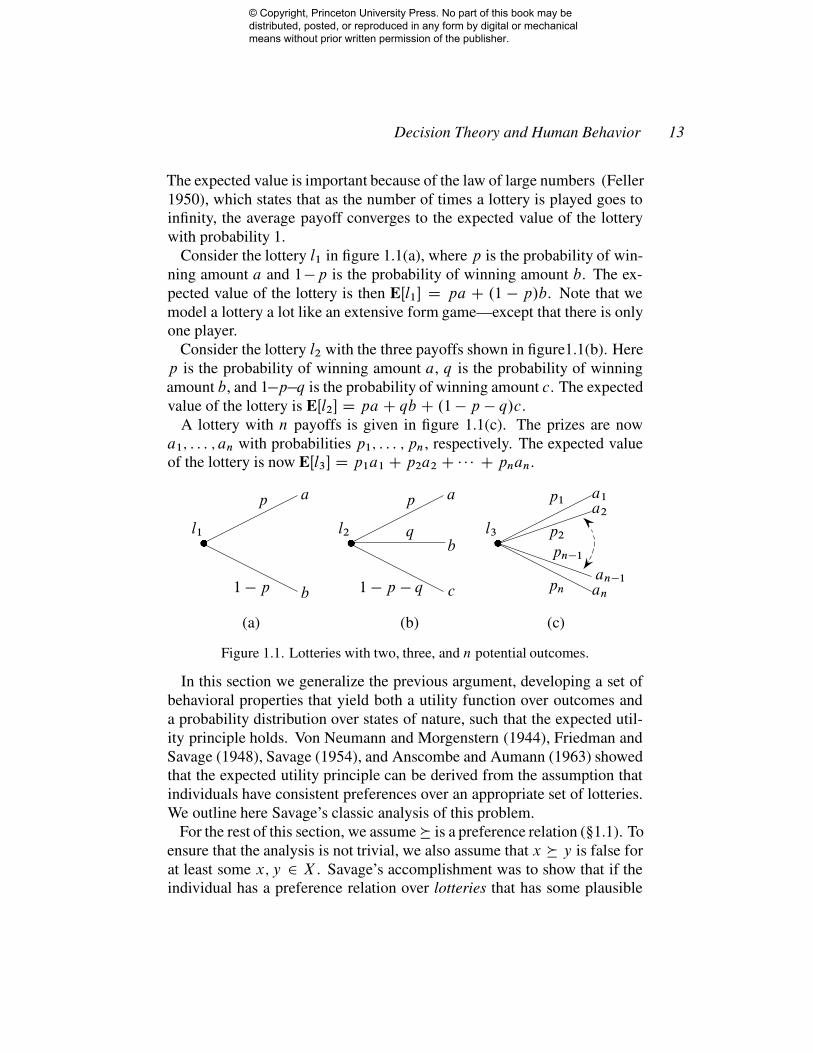
Consider the lottery l1 in figure 1.1(a), where p is the probability of win-
ning amount a and 1�p is the probability of winning amount b. The ex-
pected value of the lottery is then EŒl1� D pa C .1 � p/b. Note that we
model a lottery a lot like an extensive form game—except that there is onlyone player.
Consider the lottery l2 with the three payoffs shown in figure1.1(b). Here
p is the probability of winning amount a, q is the probability of winning
amount b, and 1�p�q is the probability of winning amount c. The expected
value of the lottery is EŒl2� D pa C qb C .1� p � q/c.
A lottery with n payoffs is given in figure 1.1(c). The prizes are now
a1; : : : ; an with probabilities p1; : : : ; pn, respectively. The expected valueof the lottery is now EŒl3� D p1a1 C p2a2 C . . . C pnan.
a1
a2
an�1
an
�
p1
p2
pn�1
pn
a
b
c
�
p
q
1 � p � q
a
b
�l1
p
1 � p
(a) (b) (c)
l2 l3
Figure 1.1. Lotteries with two, three, and n potential outcomes.
In this section we generalize the previous argument, developing a set of
behavioral properties that yield both a utility function over outcomes and
a probability distribution over states of nature, such that the expected util-
ity principle holds. Von Neumann and Morgenstern (1944), Friedman and
Savage (1948), Savage (1954), and Anscombe and Aumann (1963) showedthat the expected utility principle can be derived from the assumption that
individuals have consistent preferences over an appropriate set of lotteries.
We outline here Savage’s classic analysis of this problem.
For the rest of this section, we assume � is a preference relation (§1.1). To
ensure that the analysis is not trivial, we also assume that x � y is false for
at least some x; y 2 X . Savage’s accomplishment was to show that if theindividual has a preference relation over lotteries that has some plausible
© Copyright, Princeton University Press. No part of this book may be distributed, posted, or reproduced in any form by digital or mechanical means without prior written permission of the publisher.
14 Chapter 1
properties, then not only can the individual’s preferences be represented
by a utility function, but also we can infer the probabilities the individualimplicitly places on various events, and the expected utility principle holds
for these probabilities.
Let � be a finite set of states of nature. We call any A � � an event.
Let L be a set of lotteries, where a lottery is a function � W � ! X that
associates with each state of nature ! 2 � a payoff �.!/ 2 X . Note
that this concept of a lottery does not include a probability distribution overthe states of nature. Rather, the Savage axioms allow us to associate a
subjective prior over each state of nature !, expressing the decision maker’s
personal assessment of the probability that ! will occur. We suppose that
the individual chooses among lotteries without knowing the state of nature,
after which Nature chooses the state ! 2 � that obtains, so that if the
individual chose lottery � 2 L, his payoff is �.!/.
Now suppose the individual has a preference relation � over L (we usethe same symbol � for preferences over both outcomes and lotteries). We
seek a set of plausible properties of � over lotteries that together allow us
to deduce (a) a utility function u WX ! R corresponding to the preference
relation � over outcomes in X ; (b) a probability distribution p W � ! R
such that the expected utility principle holds with respect to the preference
relation � over lotteries and the utility function u.�/; i.e., if we define
E� ŒuIp� DX
!2�
p.!/u.�.!//; (1.5)
then for any �; � 2 L,
� � � ” E� ŒuIp� > E�ŒuIp�:
Our first condition is that � � � depends only on states of nature where �and � have different outcomes. We state this more formally as follows.
A1. For any �; �; � 0; �0 2 L, let A D f! 2 �j�.!/ ¤ �.!/g.
Suppose we also have A D f! 2 �j� 0.!/ ¤ �0.!/g. Suppose
also that �.!/ D � 0.!/ and �.!/ D �0.!/ for ! 2 A. Then
� � � , � 0 � �0.
This axiom says, reasonably enough, that the relative desirability of two
lotteries does not depend on the payoffs where the two lotteries agree. Theaxiom allows us to define a conditional preference � �A �, where A � �,
© Copyright, Princeton University Press. No part of this book may be distributed, posted, or reproduced in any form by digital or mechanical means without prior written permission of the publisher.
Decision Theory and Human Behavior 15
which we interpret as “� is strictly preferred to �, conditional on event A,”
as follows. We say � �A � if, for some � 0; �0 2 L, �.!/ D � 0.!/ and�.!/ D �0.!/ for ! 2 A, � 0.!/ D �0.!/ for ! … A, and � 0 � �0. Because
of A1, this is well defined (i.e., � �A � does not depend on the particular
� 0; �0 2 L). This allows us to define �A and �A in a similar manner. We
then define an event A � � to be null if � �A � for all �; � 2 L.
Our second condition is then the following, where we write �jA D x to
mean �.!/ D x for all ! 2 A (i.e., �jA D x means � is a lottery that paysx when A occurs).
A2. If A � � is not null, then for all x; y 2 X , �; � 2 L, �jA D x
and �jA D y, then � �A � , x � y.
This axiom says that a natural relationship between outcomes and lotteries
holds: if � pays x given event A and � pays y given event A, and if x � y,
then � �A �, and conversely.Our third condition asserts that the probability that a state of nature occurs
is independent of the outcome one receives when the state occurs. The diffi-
culty in stating this axiom is that the individual cannot choose probabilities
but only lotteries. But, if the individual prefers x to y, and if A;B � � are
events, then the individual treatsA as more probable than B if and only if a
lottery that pays x when A occurs and y when A does not occur is preferredto a lottery that pays x when B occurs and y when B does not. However,
this must be true for any x; y 2 X such that x � y, or the individual’s
notion of probability is incoherent (i.e., it depends on what particular pay-
offs we are talking about—for instance, wishful thinking, where if the prize
associated with an event increases, the individual thinks it is more likely to
occur). More formally, we have the following, where we write � D x; yjAto mean “�.!/ D x for ! 2 A and �.!/ D y for ! … A.”
A3. Suppose x � y, x0 � y 0, �; �; � 0; �0 2 L, and A;B � �.
Suppose that � D x; yjA, � D x0; y 0jA, � 0 D x; yjB , and�0 D x0; y 0jB . Then � � � 0 , � � �0.
The fourth condition is a weak version of first-order stochastic domi-
nance, which says that if one lottery has a higher payoff than another forany event, then the first is preferred to the second.
A4. For any event A, if x � �.!/ for all ! 2 A, then �jA D x
implies � �A �. Also, for any event A, if �.!/ � x for all! 2 A, and �jA D x, then � �A � .
© Copyright, Princeton University Press. No part of this book may be distributed, posted, or reproduced in any form by digital or mechanical means without prior written permission of the publisher.

16 Chapter 1
In other words, if for any event A, � D x on A pays more than the best �
can pay on A, then � �A �, and conversely.Finally, we need a technical property to show that a preference relation
can be represented by a utility function. We say nonempty sets A1; : : : ; An
form a partition of set X if the Ai are mutually disjoint (Ai \ Aj D ; for
i ¤ j ) and their union is X (i.e., A1 [ : : : [ An D X ). The technical
condition says that for any �; � 2 L, and any x 2 X , there is a partition
A1; : : : ; An of � such that, for each Ai , if we change � so that its payoffis x on Ai , then � is still preferred to �, and similarly, for each Ai , if we
change � so that its payoff is x on Ai , then � is still preferred to �. This
means that no payoff is “supergood,” so that no matter how unlikely an
event A is, a lottery with that payoff when A occurs is always preferred to
a lottery with a different payoff when A occurs. Similarly, no payoff can be
“superbad.” The condition is formally as follows.
A5. For all �; � 0; �; �0 2 L with � � �, and for all x 2 X , thereare disjoint subsets A1; : : : ; An of � such that [iAi D � and
for any Ai (a) if � 0.!/ D x for ! 2 Ai and � 0.!/ D �.!/ for
! … Ai , then � 0 � �, and (b) if �0.!/ D x for ! 2 Ai and
�0.!/ D �.!/ for ! … Ai , then � � �0.
We then have Savage’s theorem.
THEOREM 1.3 Suppose A1–A5 hold. Then there is a probability function
p on � and a utility function u WX! R such that for any �; � 2 L, � � �
if and only if E� ŒuIp� > E�ŒuIp�.
The proof of this theorem is somewhat tedious; it is sketched in Kreps
(1988).
We call the probability p the individual’s Bayesian prior, or subjective
prior and say that A1–A5 imply Bayesian rationality, because they together
imply Bayesian probability updating.
1.4 Preferences Are State-Dependent
Preferences are obviously state-dependent. For instance, my preference for
aspirin may depend on whether or not I have a headache. Similarly, I may
prefer salad to steak, but having eaten the salad, I may then prefer steak
to salad. These state-dependent aspects of preferences render the empirical
estimation of preferences somewhat delicate, but they present no theoreticalor conceptual problems.
© Copyright, Princeton University Press. No part of this book may be distributed, posted, or reproduced in any form by digital or mechanical means without prior written permission of the publisher.

Decision Theory and Human Behavior 17
We often observe that an individual makes a variety of distinct choices
under what appear to be identical circumstances. For instance, an individ-ual may vary his breakfast choice among several alternatives each morning
without any apparent pattern to his choices.
Following Luce and Suppes (1965), we represent this situation by assum-
ing the individual has a utility function of the form
u.x/ D v.x/ C �.x/ (1.6)
where � is a random error term representing the individual’s current idiosyn-
cratic taste for x. We can then express the probability that the individual
chooses x when the choice set is X as
px;X D Prf8y 2 X; y ¤ xjv.x/ C �.x/ � v.y/C �.y/g;
with the proviso that if several choices in X have the same maximal payoff,
one among them is chosen at random.Now let B D fx 2 Ajpx;A > 0g, and suppose B has at least three
elements. By the Independence of Irrelevant Alternatives, px;B D px;A > 0
for all x 2 B . We also define
pxy D Prfv.x/C �.x/ � v.y/C �.y/g;
with the proviso that when equality holds in this definition, then pxy D ½.Note that pxy ¤ 0 for x; y 2 B . We then have
py;B Dpyz
pzy
pz;B ; (1.7)
px;B Dpxz
pzx
pz;B ; (1.8)
where x; y; z 2 B are distinct, again by the Independence of Irrelevant Al-
ternatives. Dividing (1.7) by (1.8), and noting that py;B=px;B D pyx=pxy ,
we havepyx
pxy
Dpyz=pzy
pxz=pzx
: (1.9)
We can write
1 DX
y2B
py;B DX
y2B
pyx
pxy
px;B;
© Copyright, Princeton University Press. No part of this book may be distributed, posted, or reproduced in any form by digital or mechanical means without prior written permission of the publisher.
18 Chapter 1
so
px;B D1
P
y2B pyx=pxy
Dpxz=pzx
P
y2B pyx=pzy
; (1.10)
where the second equality comes from (1.9).
Let us write
w.x; z/ D ˇ lnpxz=pzx;
so (1.10) becomes
px;B Deˇw.x;z/
P
y2B eˇw.y;z/
: (1.11)
But by the Independence of Irrelevant Alternatives, this expression must be
independent of our choice of z, so if we writew.x/ D lnpxz for a arbitrary
z 2 B ,we have
px;B Deˇw.x/
P
y2B eˇw.y/
: (1.12)
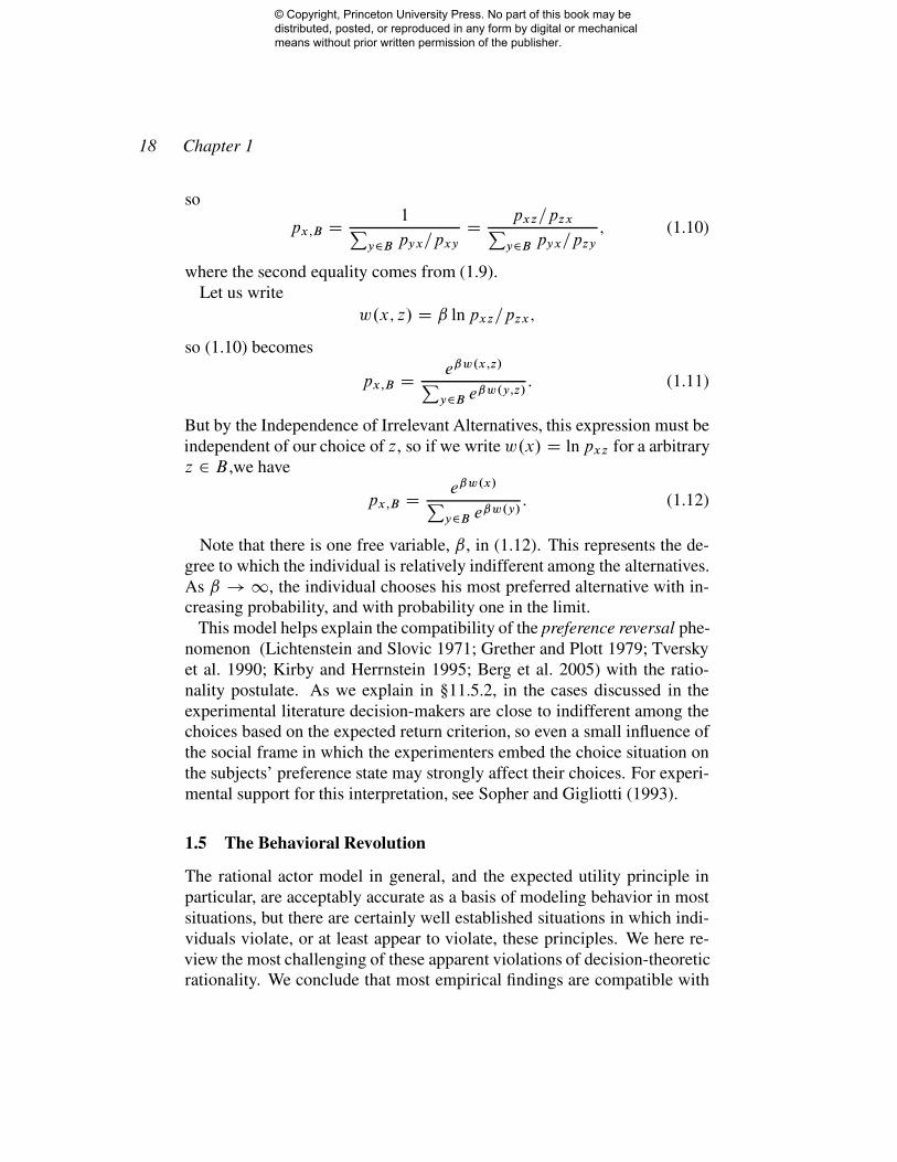
Note that there is one free variable, ˇ, in (1.12). This represents the de-
gree to which the individual is relatively indifferent among the alternatives.
As ˇ ! 1, the individual chooses his most preferred alternative with in-creasing probability, and with probability one in the limit.
This model helps explain the compatibility of the preference reversal phe-
nomenon (Lichtenstein and Slovic 1971; Grether and Plott 1979; Tversky
et al. 1990; Kirby and Herrnstein 1995; Berg et al. 2005) with the ratio-
nality postulate. As we explain in §11.5.2, in the cases discussed in the
experimental literature decision-makers are close to indifferent among thechoices based on the expected return criterion, so even a small influence of
the social frame in which the experimenters embed the choice situation on
the subjects’ preference state may strongly affect their choices. For experi-
mental support for this interpretation, see Sopher and Gigliotti (1993).
1.5 The Behavioral Revolution
The rational actor model in general, and the expected utility principle in
particular, are acceptably accurate as a basis of modeling behavior in most
situations, but there are certainly well established situations in which indi-
viduals violate, or at least appear to violate, these principles. We here re-
view the most challenging of these apparent violations of decision-theoreticrationality. We conclude that most empirical findings are compatible with
© Copyright, Princeton University Press. No part of this book may be distributed, posted, or reproduced in any form by digital or mechanical means without prior written permission of the publisher.

Decision Theory and Human Behavior 19
the rational actor model so long as the proper choice set is assumed. In par-
ticular, actor preferences are generically dependent on the arousal state ofthe decision-maker, the social frame in which decisions are made, and the
original position from which the decision-maker evaluates the available al-
ternatives. For an elaboration of these points in the context of the possibility
for unifying the behavioral sciences, see Ch. 11.
Our treatment of these issues may appear to the reader to go against the
grain of popular opinion concerning the rather stunning findings of behav-ioral game theory, from which many conclude that human decision-making
is fundamentally irrational (Ariely 2010). In fact, the apparent paradoxes
of choice are closely akin to optical illusions in the theory of vision. Both
afford great insight into how humans model the external world. However,
just as the existence of optical illusions do not lead us to believe that hu-
man vision is a fundamental distortion of reality, neither should behavioral
inconsistencies lead us to believe in the fundamental irrationality of humanchoice behavior.
1.5.1 The Allais and Ellsberg Paradoxes
Although most decision theorists consider the expected utility principle ac-
ceptably accurate as a basis of modeling behavior, there are certainly well
established situations in which individuals violate it. Machina (1987) re-
views this body of evidence and presents models to deal with them. We
sketch here the most famous of these anomalies, the Allais paradox andthe Ellsberg paradox. They are, of course, not paradoxes at all but simply
empirical regularities that do not fit the expected utility principle.
Maurice Allais (1953) offered the following scenario. There are two
choice situations in a game with prizes x D $2,500,000, y D $500,000,
and z D $0. The first is a choice between lotteries � D y and � 0 D0:1xC 0:89yC 0:01z. The second is a choice between � D 0:11yC 0:89z
and �0 D 0:1x C 0:9z. Most people, when faced with these two choicesituations, choose � � � 0 and �0 � �. Which would you choose?
This pair of choices is not consistent with the expected utility principle.
To see this, let us write uh D u.2500000/, um D u.500000/, and ul Du.0/. Then if the expected utility principle holds, � � � 0 implies um >
0:1uh C 0:89um C 0:01ul , so 0:11um > 0:10uh C 0:01ul , which implies
(adding 0:89ul to both sides) 0:11um C 0:89ul > 0:10uh C 0:9ul , whichsays � � �0.
© Copyright, Princeton University Press. No part of this book may be distributed, posted, or reproduced in any form by digital or mechanical means without prior written permission of the publisher.
20 Chapter 1
Why do people make this mistake? Perhaps because of regret, which does
not mesh well with the expected utility principle (Loomes 1988; Sugden1993). If you choose � 0 in the first case and you end up getting nothing,
you will feel really foolish, whereas in the second case you are probably
going to get nothing anyway (not your fault), so increasing the chances of
getting nothing a tiny bit (0.01) gives you a good chance (0.10) of winning
the really big prize. Or perhaps because of loss aversion (§1.5.3), because
in the first case, the anchor point (the most likely outcome) is $500,000,while in the second case the anchor is $0. Loss-averse individuals then
shun � 0, which gives a positive probability of loss whereas in the second
case, neither lottery involves a loss, from the standpoint of the most likely
outcome.
The Allais paradox is an excellent illustration of problems that can arise
when a lottery is consciously chosen by an act of will and one knows that
one has made such a choice. The regret in the first case arises because ifone chose the risky lottery and the payoff was zero, one knows for certain
that one made a poor choice, at least ex post. In the second case, if one
received a zero payoff, the odds are that it had nothing to do with one’s
choice. Hence, there is no regret in the second case. But in the real world,
most of the lotteries we experience are chosen by default, not by acts of
will. Thus, if the outcome of such a lottery is poor, we feel bad because ofthe poor outcome but not because we made a poor choice.
Another classic violation of the expected utility principle was suggested
by Daniel Ellsberg (1961). Consider two urns. Urn A has 51 red balls and
49 white balls. Urn B also has 100 red and white balls, but the fraction of
red balls is unknown. One ball is chosen from each urn but remains hidden
from sight. Subjects are asked to choose in two situations. First, a subjectcan choose the ball from urn A or urn B , and if the ball is red, the subject
wins $10. In the second situation, the subject can choose the ball from urn
A or urn B , and if the ball is white, the subject wins $10. Many subjects
choose the ball from urn A in both cases. This violates the expected utility
principle no matter what probability the subject places on the probability p
that the ball from urn B is white. For in the first situation, the payoff from
choosing urnA is 0:51u.10/C0:49u.0/ and the payoff from choosing urnBis .1�p/u.10/Cpu.0/, so strictly preferring urnAmeans p > 0:49. In the
second situation, the payoff from choosing urn A is 0:49u.10/C 0:51u.0/
and the payoff from choosing urn B is pu.10/ C .1 � p/u.0/, so strictly
© Copyright, Princeton University Press. No part of this book may be distributed, posted, or reproduced in any form by digital or mechanical means without prior written permission of the publisher.

Decision Theory and Human Behavior 21
preferring urn A means p < 0:49. This shows that the expected utility
principle does not hold.Whereas the other proposed anomalies of classical decision theory can be
interpreted as the failure of linearity in probabilities, regret, loss aversion,
and epistemological ambiguities, the Ellsberg paradox appears to strike
even more deeply because it implies that humans systematically violate the
following principle of first-order stochastic dominance (FOSD).
Let p.x/ and q.x/ be the probabilities of winning x or more in
lotteries A and B , respectively. If p.x/ � q.x/ for all x, then
A � B .
The usual explanation of this behavior is that the subject knows the prob-
abilities associated with the first urn, while the probabilities associated withthe second urn are unknown, and hence there appears to be an added degree
of risk associated with choosing from the second urn rather than the first. If
decision makers are risk-averse and if they perceive that the second urn is
considerably riskier than the first, they will prefer the first urn. Of course,
with some relatively sophisticated probability theory, we are assured that
there is in fact no such additional risk, it is hardly a failure of rationality for
subjects to come to the opposite conclusion. The Ellsberg paradox is thusa case of performance error on the part of subjects rather than a failure of
rationality.
1.5.2 Risk and the Shape of the Utility Function
If � is defined over X , we can say nothing about the shape of a utility func-
tion u.�/ representing � because, by Theorem 1.2, any increasing function
of u.�/ also represents �. However, if � is represented by a utility functionu.x/ satisfying the expected utility principle, then u.�/ is determined up to
an arbitrary constant and unit of measure.6
THEOREM 1.4 Suppose the utility function u.�/ represents the preference
relation � and satisfies the expected utility principle. If v.�/ is another
6Because of this theorem, the difference between two utilities means nothing. We thus
say utilities over outcomes are ordinal, meaning we can say that one bundle is preferred to
another, but we cannot say by how much. By contrast, the next theorem shows that utilities
over lotteries are cardinal, in the sense that, up to an arbitrary constant and an arbitrarypositive choice of units, utility is numerically uniquely defined.
© Copyright, Princeton University Press. No part of this book may be distributed, posted, or reproduced in any form by digital or mechanical means without prior written permission of the publisher.

22 Chapter 1
G
HIF
DC
E.u.x//
u.x/
�
y
�
x
u.Ex/u.y/
�
u.x/�
E.x/
A
B
E
Figure 1.2. A concave utility function
utility function representing �, then there are constants a; b 2 R with a > 0
such that v.x/ D au.x/C b for all x 2 X .
For a proof of this theorem, see Mas-Colell, Whinston, and Green (1995,
p. 173).
If X D R, so the payoffs can be considered to be money, and utility
satisfies the expected utility principle, what shape do such utility functions
have? It would be nice if they were linear in money, in which case expected
utility and expected value would be the same thing (why?). But generallyutility is strictly concave, as illustrated in figure 1.2. We say a function
u WX ! R is strictly concave if, for any x; y 2 X and any p 2 .0; 1/, we
have pu.x/ C .1 � p/u.y/ < u.px C .1 � p/y/. We say u.x/ is weakly
concave, or simply concave, if u.x/ is either strictly concave or linear, in
which case the above inequality is replaced by pu.x/ C .1 � p/u.y/ Du.px C .1 � p/y/.
If we define the lottery � as paying x with probability p and y with
probability 1 � p, then the condition for strict concavity says that the ex-
pected utility of the lottery is less than the utility of the expected value of
the lottery, as depicted in figure 1.2. To see this, note that the expected
value of the lottery is E D px C .1 � p/y, which divides the line seg-
ment between x and y into two segments, the segment xE having length
.pxC .1�p/y/� x D .1�p/.y � x/ and the segment Ey having lengthy� .pxC .1�p/y/ D p.y�x/. Thus, E divides Œx; y� into two segments
whose lengths have the ratio .1� p/=p. From elementary geometry, it fol-
lows that B divides segment ŒA; C � into two segments whose lengths have
the same ratio. By the same reasoning, point H divides segments ŒF;G�
into segments with the same ratio of lengths. This means that point H has
the coordinate value pu.x/C .1�p/u.y/, which is the expected utility ofthe lottery. But by definition, the utility of the expected value of the lottery
© Copyright, Princeton University Press. No part of this book may be distributed, posted, or reproduced in any form by digital or mechanical means without prior written permission of the publisher.
Decision Theory and Human Behavior 23
is at D, which lies above H . This proves that the utility of the expected
value is greater than the expected value of the lottery for a strictly concaveutility function. This is known as Jensen’s inequality.
What are good candidates for u.x/? It is easy to see that strict concav-
ity means u00.x/ < 0, providing u.x/ is twice differentiable (which we
assume). But there are lots of functions with this property. According to
the famous Weber-Fechner law of psychophysics, for a wide range of sen-
sory stimuli and over a wide range of levels of stimulation, a just noticeablechange in a stimulus is a constant fraction of the original stimulus. If this
holds for money, then the utility function is logarithmic.
We say an individual is risk-averse if the individual prefers the expected
value of a lottery to the lottery itself (provided, of course, the lottery does
not offer a single payoff with probability 1, which we call a sure thing). We
know, then, that an individual with utility function u.�/ is risk-averse if and
only if u.�/ is concave.7 Similarly, we say an individual is risk-loving if heprefers any lottery to the expected value of the lottery, and risk-neutral if he
is indifferent between a lottery and its expected value. Clearly, an individual
is risk-neutral if and only if he has linear utility.
Does there exist a measure of risk aversion that allows us to say when
one individual is more risk-averse than another, or how an individual’s risk
aversion changes with changing wealth? We may define individual A to bemore risk-averse than individual B if whenever A prefers a lottery to an
amount of money x, B will also prefer the lottery to x. We say A is strictly
more risk-averse than B if he is more risk-averse and there is some lottery
that B prefers to an amount of money x but such that A prefers x to the
lottery.
Clearly, the degree of risk aversion depends on the curvature of the utilityfunction (by definition the curvature of u.x/ at x is u00.x/), but because
u.x/ and v.x/ D au.x/C b (a > 0) describe the same behavior, although
v.x/ has curvature a times that of u.x/, we need something more sophis-
ticated. The obvious candidate is �u.x/ D �u00.x/=u0.x/, which does not
depend on scaling factors. This is called the Arrow-Pratt coefficient of ab-
7One may ask why people play government-sponsored lotteries or spend money at
gambling casinos if they are generally risk-averse. The most plausible explanation is that
people enjoy the act of gambling. The same woman who will have insurance on her
home and car, both of which presume risk aversion, will gamble small amounts of money
for recreation. An excessive love for gambling, of course, leads an individual either topersonal destruction or to wealth and fame (usually the former).
© Copyright, Princeton University Press. No part of this book may be distributed, posted, or reproduced in any form by digital or mechanical means without prior written permission of the publisher.

24 Chapter 1
solute risk aversion, and it is exactly the measure that we need. We have
the following theorem.
THEOREM 1.5 An individual with utility function u.x/ is more risk-averse
than an individual with utility function v.x/ if and only if �u.x/ > �v.x/
for all x.
For example, the logarithmic utility function u.x/ D ln.x/ has Arrow-
Pratt measure �u.x/ D 1=x, which decreases with x; i.e., as the indi-
vidual becomes wealthier, he becomes less risk-averse. Studies show that
this property, called decreasing absolute risk aversion, holds rather widely(Rosenzweig and Wolpin 1993; Saha et al. 1994; Nerlove and Soedjiana
1996). Another increasing concave function is u.x/ D xa for a 2 .0; 1/,
for which �u.x/ D .1� a/=x, which also exhibits decreasing absolute risk
aversion. Similarly, u.x/ D 1 � x�a (a > 0) is increasing and concave,
with �u.x/ D �.a C 1/=x, which again exhibits decreasing absolute risk
aversion. This utility has the additional attractive property that utility isbounded: no matter how rich you are, u.x/ < 1.8 Yet another candidate
for a utility function is u.x/ D 1 � e�ax for some a > 0. In this case
�u.x/ D a, which we call constant absolute risk aversion.
Another commonly used term is coefficient of relative risk aversion,
�u.x/ D �u.x/=x. Note that for any of the utility functions u.x/ D ln.x/,
u.x/ D xa for a 2 .0; 1/, and u.x/ D 1 � x�a (a > 0), �u.x/ is constant,which we call constant relative risk aversion. For u.x/ D 1�e�ax (a > 0),
we have �u.x/ D a=x, so we have decreasing relative risk aversion.
1.5.3 Prospect Theory
A large body of experimental evidence indicates that people value payoffs
according to whether they are gains or losses compared to their current
status quo position. This is related to the notion that individuals adjust to
an accustomed level of income, so that subjective well-being is associated
more with changes in income rather than with the level of income. See,
for instance, Helson (1964), Easterlin (1974, 1995), Lane (1991, 1993),
and Oswald (1997). Indeed, people appear to be about twice as averseto taking losses as to enjoying an equal level of gains (Kahneman et al.
8If utility is unbounded, it is easy to show that there is a lottery that you would be
willing to give all your wealth to play no matter how rich you are. This is not plausiblebehavior.
© Copyright, Princeton University Press. No part of this book may be distributed, posted, or reproduced in any form by digital or mechanical means without prior written permission of the publisher.
Decision Theory and Human Behavior 25
1990; Tversky and Kahneman 1981b). This means, for instance, that an
individual may attach zero value to a lottery that offers an equal chanceof winning $1000 and losing $500. This also implies that people are risk-
loving over losses while they remain risk-averse over gains (§1.5.2 explains
the concept of risk aversion). For instance, many individuals choose a 25%
probability of losing $2000 rather than a 50% chance of losing $1000 (both
have the same expected value, of course, but the former is riskier).
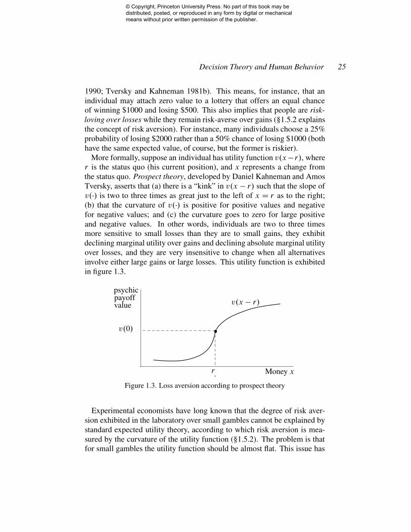
More formally, suppose an individual has utility function v.x�r/, wherer is the status quo (his current position), and x represents a change from
the status quo. Prospect theory, developed by Daniel Kahneman and Amos
Tversky, asserts that (a) there is a “kink” in v.x � r/ such that the slope of
v.�/ is two to three times as great just to the left of x D r as to the right;
(b) that the curvature of v.�/ is positive for positive values and negative
for negative values; and (c) the curvature goes to zero for large positive
and negative values. In other words, individuals are two to three timesmore sensitive to small losses than they are to small gains, they exhibit
declining marginal utility over gains and declining absolute marginal utility
over losses, and they are very insensitive to change when all alternatives
involve either large gains or large losses. This utility function is exhibited
in figure 1.3.
v.0/
Money x
psychic
v.x � r/
�
r
valuepayoff
Figure 1.3. Loss aversion according to prospect theory
Experimental economists have long known that the degree of risk aver-
sion exhibited in the laboratory over small gambles cannot be explained by
standard expected utility theory, according to which risk aversion is mea-
sured by the curvature of the utility function (§1.5.2). The problem is thatfor small gambles the utility function should be almost flat. This issue has
© Copyright, Princeton University Press. No part of this book may be distributed, posted, or reproduced in any form by digital or mechanical means without prior written permission of the publisher.

26 Chapter 1
been formalized by Rabin (2000). Consider a lottery that imposes a $100
loss and offers a $125 gain with equal probability p D 1=2. Most subjectsin the laboratory reject this lottery. Rabin shows that if this is true for all
expected lifetime wealth levels less than $300,000, then in order to induce
a subject to sustain a loss of $600 with probability 1/2, you would have to
offer him a gain of at least $36,000,000,000 with probability 1/2. This is,
of course, quite absurd.
There are many regularities in empirical data on human behavior that fitprospect theory very well (Kahneman and Tversky 2000). For instance,
returns on stocks in the United States have exceeded the returns on bonds
by about 8 percentage points, averaged over the past 100 years. Assum-
ing investors are capable of correctly estimating the shape of the return
schedule, if this were due to risk aversion alone, then the average individ-
ual would be indifferent between a sure $51,209 and a lottery that paid
$50,000 with probability 1/2 and paid $100,000 with probability 1/2. It is,of course, quite implausible that more than a few individuals would be this
risk-averse. However, a loss aversion coefficient (the ratio of the slope of
the utility function over losses at the kink to the slope over gains) of 2.25 is
sufficient to explain this phenomenon. This loss aversion coefficient is very
plausible based on experiments.
In a similar vein, people tend to sell stocks when they are doing well buthold onto stocks when they are doing poorly. A kindred phenomenon holds
for housing sales: homeowners are extremely averse to selling at a loss and
sustain operating, tax, and mortgage costs for long periods of time in the
hope of obtaining a favorable selling price.
One of the earliest examples of loss aversion is the ratchet effect discov-
ered by James Duesenberry, who noticed that over the business cycle, whentimes are good, people spend all their additional income, but when times
start to go bad, people incur debt rather than curb consumption. As a result,
there is a tendency for the fraction of income saved to decline over time. For
instance, in one study unionized teachers consumed more when next year’s
income was going to increase (through wage bargaining) but did not con-
sume less when next year’s income was going to decrease. We can explain
this behavior with a simple loss aversion model. A teacher’s utility can bewritten as u.ct � rt /C st.1C �/, where ct is consumption in period t , st
is savings in period t , � is the rate of interest on savings, and rt is the ref-
erence point (status quo point) in period t . This assumes that the marginal
utility of savings is constant, which is a very good approximation. Now
© Copyright, Princeton University Press. No part of this book may be distributed, posted, or reproduced in any form by digital or mechanical means without prior written permission of the publisher.

Decision Theory and Human Behavior 27
suppose the reference point changes as follows: rtC1 D ˛rt C .1 � ˛/ct ,
where ˛ 2 Œ0; 1� is an adjustment parameter (˛ D 1 means no adjustmentand ˛ D 0 means complete adjustment to last year’s consumption). Note
that when consumption in one period rises, the reference point in the next
period rises, and conversely.
Now, dropping the time subscripts and assuming the individual has in-
comeM , so c C s D M , the individual chooses c to maximize
u.c � r/C .M � c/.1C �/:
This gives the first order condition u0.c � r/ D 1 C �. Because this must
hold for all r , we can differentiate totally with respect to r , getting
u00.c � r/dc
drD u00.c � r/:
This shows that dc=dr D 1 > 0, so when the individual’s reference point
rises, his consumption rises an equal amount.
One general implication of prospect theory is a status quo bias, according
to which people often prefer the status quo over any of the alternatives butif one of the alternatives becomes the status quo, that too is preferred to any
of the alternatives (Kahneman et al. 1991). Status quo bias makes sense if
we recognize that any change can involve a loss, and because on the average
gains do not offset losses, it is possible that any one of a number of alter-
natives might be preferred if it is the status quo. For instance, if employers
make joining a 401k savings plan the default position, almost all employeesjoin. If not joining is made the default position, most employees do not join.
Similarly, if the state automobile insurance commission declares one type
of policy the default option and insurance companies ask individual poli-
cyholders how they would like to vary from the default, the policyholders
tend not to vary, no matter what the default is (Camerer 2000).
Another implication of prospect theory is the endowment effect (Kahne-
man et al. 1991), according to which people place a higher value on whatthey possess than they place on the same things when they do not possess
them. For instance, if you win a bottle of wine that you could sell for $200,
you may drink it rather than sell it, but you would never think of buying a
$200 bottle of wine. A famous experimental result exhibiting the endow-
ment effect was the “mug” experiment described by Kahneman, Knetsch
and Thaler (1990). College student subjects given coffee mugs with theschool logo on them demand a price two to three times as high to sell the
© Copyright, Princeton University Press. No part of this book may be distributed, posted, or reproduced in any form by digital or mechanical means without prior written permission of the publisher.
28 Chapter 1
mugs as those without mugs are willing to pay to buy the mugs. There is
evidence that people underestimate the endowment effect and hence can-not appropriately correct for it in their choice behavior (Loewenstein and
Adler 1995).
Yet another implication of prospect theory is the existence of a framing
effect, whereby one form of a lottery is strictly preferred to another even
though they have the same payoffs with the same probabilities (Tversky
and Kahneman 1981a). For instance, people prefer a price of $10 plus a$1 discount to a price of $8 plus a $1 surcharge. Framing is, of course,
closely associated with the endowment effect because framing usually in-
volves privileging the initial state from which movements are assessed.
The framing effect can seriously distort effective decision making. In par-
ticular, when it is not clear what the appropriate reference point is, decision
makers can exhibit serious inconsistencies in their choices. Kahneman and
Tversky give a dramatic example from health care policy. Suppose we facea flu epidemic in which we expect 600 people to die if nothing is done.
If program A is adopted, 200 people will be saved, while if program B is
adopted, there is a 1/3 probability 600 will be saved and a 2/3 probability
no one will be saved. In one experiment, 72% of a sample of respondents
preferred A to B. Now suppose that if program C is adopted, 400 people
will die, while if program D is adopted there is a 1/3 probability nobodywill die and a 2/3 probability 600 people will die. Now, 78% of respon-
dents preferred D to C, even though A and C are equivalent in terms of the
probability of each final state, and B and D are similarly equivalent. How-
ever, in the choice between A and B, alternatives are over gains, whereas
in the choice between C and D, the alternatives are over losses, and people
are loss-averse. The inconsistency stems from the fact that there is no natu-ral reference point for the decision maker, because the gains and losses are
experienced by others, not by the decision maker himself.
The brilliant experiments by Kahneman, Tversky, and their coworkers
clearly show that humans exhibit systematic biases in the way they make
decisions. However, it should be clear that none of the above examples
illustrates preference inconsistency once the appropriate parameter (cur-
rent time, current position, status quo point) is admitted into the preferencefunction. This point is formally demonstrated in Sugden (2003). Sugden
considers a preference relation of the form f � gjh, which means “lot-
tery f is weakly preferred to lottery g when one’s status quo position is
lottery h.” Sugden shows that if several conditions on this preference re-
© Copyright, Princeton University Press. No part of this book may be distributed, posted, or reproduced in any form by digital or mechanical means without prior written permission of the publisher.
Decision Theory and Human Behavior 29
lation, most of which are direct generalizations of the Savage conditions
(§1.3), obtain, then there is a utility function u.x; z/ such that f � gjh ifand only if EŒu.f; h/� � EŒu.g; h/�, where the expectation is taken over the
probability of events derived from the preference relation.
1.5.4 Heuristics and Biases in Decision Making
Laboratory testing of the standard economic model of choice under un-
certainty was initiated by the psychologists Daniel Kahneman and Amos
Tversky. In a famous article in the journal Science, Tversky and Kahneman
(1974) summarized their early research as follows:
How do people assess the probability of an uncertain event orthe value of an uncertain quantity? . . . people rely on a lim-
ited number of heuristic principles which reduce the complex
tasks of assessing probabilities and predicting values to simpler
judgmental operations. In general, these heuristics are quite
useful, but sometimes they lead to severe and systematic er-
rors.
Subsequent research has strongly supported this assessment (Kahneman et
al. 1982; Shafir and Tversky 1992; Shafir and Tversky 1995). Although westill do not have adequate models of these heuristics, we can make certain
generalizations.
First, in judging whether an event A or object A belongs to a class or pro-
cess B , one heuristic that people use is to consider whether A is represen-
tative of B but consider no other relevant facts, such as the frequency of B .
For instance, if informed that an individual has a good sense of humor and
likes to entertain friends and family, and asked if the individual is a profes-sional comic or a clerical worker, people are more likely to say the former.
This is despite the fact that a randomly chosen person is much more likely
to be a clerical worker than a professional comic, and many people have a
good sense of humor, so there are many more clerical workers satisfying
the description than professional comics.
A particularly pointed example of this heuristic is the famous Linda theBank Teller problem (Tversky and Kahneman 1983). Subjects are given
the following description of a hypothetical person named Linda:
Linda is 31 years old, single, outspoken, and very bright. Shemajored in philosophy. As a student, she was deeply concerned
© Copyright, Princeton University Press. No part of this book may be distributed, posted, or reproduced in any form by digital or mechanical means without prior written permission of the publisher.
30 Chapter 1
with issues of discrimination and social justice and also partic-
ipated in antinuclear demonstrations.
The subjects were then asked to rank-order eight statements about Linda
according to their probabilities. The statements included the following two:
Linda is a bank teller.Linda is a bank teller and is active in the feminist movement.
More than 80% of the subjects—graduate and medical school students with
statistical training and doctoral students in the decision science program
at Stanford University’s business school—ranked the second statement as
more probable than the first. This seems like a simple logical error be-
cause every bank teller feminist is also a bank teller. It appears, once again,that subjects measure probability by representativeness and ignore baseline
frequencies.
However, there is another interpretation according to which the subjects
are correct in their judgments. Let p and q be properties that every member
of a population either has or does not have. The standard definition of “the
probability that member x is p” is the fraction of the population for whichp is true. But an equally reasonable definition is “the probability that x is
a member of a random sample of the subset of the population for which p
is true.” In other words, the subjects interpret the question as asking for the
conditional probability that an individual is Linda given that the individual
is a banker vs. is a feminist banker. Obviously, given the information, the
latter alternative is much more likely.According to the standard definition, the probability of p and q cannot be
greater than the probability of p. But, according to the second, the opposite
inequality can hold: x might be more likely to appear in a random sample of
individuals who are both p and q than in a random sample of the same size
of individuals who are p. In other words, the probability that a randomly
chosen bank teller is Linda is probably much lower than the probability that
a randomly chosen feminist bank teller is Linda. Another way of expressingthis point is that the probability that a randomly chosen member of the set
“is a feminist bank teller” may be Linda is greater than the probability that
a randomly chosen member of the set “is a bank teller,” is Linda.
A second heuristic is that in assessing the frequency of an event, peo-
ple take excessive account of information that is easily available or highly
salient, even though a selective bias is obviously involved. For this rea-son, people tend to overestimate the probability of rare events because such
© Copyright, Princeton University Press. No part of this book may be distributed, posted, or reproduced in any form by digital or mechanical means without prior written permission of the publisher.
Decision Theory and Human Behavior 31
events are highly newsworthy while nonoccurrences are not reported. Thus,
people worry much more about dying in an accident while flying than theydo while driving, even though air travel is much safer than automobile
travel.
A third heuristic in problem solving is to start from an initial guess, cho-
sen for its representativeness or salience, and adjust upward or downward
toward a final figure. This is called anchoring because there is a tendency
to underadjust, so the result is too close to the initial guess. Probably asa result of anchoring, people tend to overestimate the probability of con-
junctions (p and q) and underestimate the probability of disjunctions (p or
q).
For an instance of the former, a person who knows an event occurs with
95% probability may overestimate the probability that the event occurs 10
times in a row, suggesting a probability of 90%. The actual probability is
about 60%. In this case the individual starts with 95% and does not adjustdownward sufficiently. Similarly, if a daily event has a failure one time in
a thousand, people will underestimate the probability that a failure occurs
at least once in a year, suggesting a figure of 5%. The actual probability is
30.5%. Again, the individual starts with 0.1% and doesn’t adjust upward
enough.
A fourth heuristic is that people prefer objective probability distributionsto subjective distributions derived from applying probabilistic principles,
such as the principle of insufficient reason, which says that if you are com-
pletely ignorant as to which of several outcomes will occur, you should
treat them as equally probable. For example, if you give a subject a prize
for drawing a red ball from an urn containing red and white balls, the sub-
ject will pay to have the urn contain 50% red balls rather than contain anindeterminate percentage of red balls. This is the famous Ellsberg paradox,
analyzed in §1.5.1.
Choice theorists often express dismay over the failure of people to apply
the laws of probability and conform to normative decision theory. Yet, peo-
ple may be applying rules that serve them well in daily life. It takes many
years of study to feel at home with the laws of probability, the understand-
ing of which is the product of the last couple of hundred years of scientificresearch. Moreover, it is costly, in terms of time and effort, to apply these
laws even if we know them. Of course, if the stakes are high enough, it is
worthwhile to make the effort or engage an expert who will do it for you.
But generally, as Kahneman and Tversky suggest, we apply a set of heuris-
© Copyright, Princeton University Press. No part of this book may be distributed, posted, or reproduced in any form by digital or mechanical means without prior written permission of the publisher.

32 Chapter 1
tics that more or less get the job done. Among the most prominent heuristics
is simply imitation: decide what class of phenomenon is involved, find outwhat people normally do in that situation, and do it. If there is some mech-
anism leading to the survival and growth of relatively successful behaviors,
and if the problem in question recurs with sufficient regularity, the choice-
theoretic solution will describe the winner of a dynamic social process of
trial, error, and imitation.
Should we expect people to conform to the axioms of choice theory—transitivity, independence from irrelevant alternatives, the sure-thing prin-
ciple, and the like? Where we know that individuals are really optimizing,
and have expertise in decision theory, we doubtless should. But this applies
only to a highly restricted range of actions. In more general settings we
should not. We might have recourse to Darwinian analysis, demonstrat-
ing that under the appropriate conditions individuals who are genetically
constituted to obey the axioms of choice theory are better fit to solve gen-eral decision-theoretic problems and hence will emerge triumphant through
an evolutionary dynamic. But human beings did not evolve facing general
decision-theoretic problems. Rather, they faced a few specific decision-
theoretic problems associated with survival in small social groups. We may
have to settle for modeling these specific choice contexts to discover how
our genetic constitution and cultural tools interact in determining choiceunder uncertainty.
© Copyright, Princeton University Press. No part of this book may be distributed, posted, or reproduced in any form by digital or mechanical means without prior written permission of the publisher.


![УДК519.248[33+301+159.9] Eventological Theory of Decision ... · The eventological theory of decision-making, the theory of event-based decision-making is a theory of decision-making](https://img.pdfslide.net/doc/110x75/5f75675b02834a3bf806f32d/519248333011599-eventological-theory-of-decision-the-eventological.jpg)