Embed Size (px)
Citation preview

..
CS 116 A. I. 72
CO CO o o 00
Q
THE KINEMATICS OF MANIPULATORS
UNDER COMPUTER CONTROL
BY
DONALD LEE PIEPER
SPONSORED BY
ADVANCED RESEARCH PROJECTS AGENCY ARPA ORDER NO. 457
OCTOBER 24, 1968
■ da ■ ' -.oved ile; its
distribn' on ir- uuLmiUid icr pü:c reit U
COMPUTER SCIENCE DEPARTMENT
School of Humanities and Sciences
STANFORD UNIVERSITY
"
^ JWN?
Reproduced by the CLEARINGHOUSE
lor Federal Scientific & Technical Information Springfield Va 22151 1°

:i
D ß :1 D
:
::
:
;
a D Q
0 11
STANFORD ARTIFICIAL INTELLIGENCE REPORT October 24, 1968 MEMO NO. AI-72
THE KINEMATICS OF MANIPUIATCRS UNDER COMPUTER CONTROL
by Donald L. Pieper
ABSTRACT: The kinematics of manipulators is studied. A model is presented which allows for the systematic description of new and existing manipulators.
Six degree-of-freedorn manipule ors are studied. Several solutions to the problem of finding the manipulator configuration leading to a specified position and orien- tation are presented. Numerical as well as explicit solutions are given. The problem of positioning a multi- link digital arm is also discussed.
Given the solution to the position problem, a set of heuristics is developed for moving a six degree-of- freedom manipulator from an initial position to a final position through a space containing obstacles. This results in a computer program shown to be able to direct a manipulator around obstacles.
The research reported here was supported in part by the Advanced Research Projects Agency of the Office of the Secretary of Defense (SD"183).

[
THE KINEMATICS OF MANIPUIATCRS UNDER COMPUTER CONTROL
ABSTRACT
This dissertation Is concerned with the kinematic analysis of
computer controlled manipulators. Existing Industrial and experimental
manipulators are cataloged according to a new model which allows for the
systematic description of both existing and new manipulators.
This work deals mainly with manipulators consisting of six degree-
of-freedom open chains of articulated links with either turning (revolute)
or sliding (prismatic) Joints. The last link called the "hand" is the
free end of the manipulator and has additional motion capabilities which
I make it possible to grasp objects.
The following problem is discussed: given the desired hand position
and orientation along with the various link parameters defining the
structure, what are the values of the manipulator variables that place
the hand at the desired position with the desired orientation? Solutions
to this problem are presented for any six degree-of-freedom manipulator
with three revolute Joints whose axes intersect at a point, provided the
remaining three joints are revolute or prismatic pairs. These results
can be expressed as a fourth degree polynomial in -«ne unknown, and closed
form expressions for the remaining unknowns.
It is shown that this is equivalent to the kinematic analysis of all
single loop five-bar mechanisms with one sph« rical Joint and four Joints
which are revolute or prismatic pairs. The extension to the case where
only one pair of axes Intersect is discussed. A similar solution for I
any manipulator with three prismatic Joints is also given.
[
I I I
^»»•"«■■■B»
■
A numerical procedure based on velocity methods Is developed to
analyze manipulators which cannot be "solved" explicitly. This pro-
cedure Is found to be superior to the widely used Newton-Raphson
technique.
The problem of positioning a "digital arm" (I.e., a multl-Unk
manipulator where each Joint Is only capable of several digital steps)
Is discussed. A simple searching algorithm using a look-ahead scheme
Is developed. A two-dimensional model and three-dimensional model are
studied.
Given the solution to the position problem, a set of heuristics Is
developed for moving a six degree-of-free dorn manipulator from an Initial
position to a final position through a space containing obstacles. A
mathematical model of objects Is developed so that possible conflict
between objects and any link of the manipulator can be detected and
avoided.
Some considerations In choosing a manipulator for use with a
computer are discussed. A set of computer programs - In FCRTRAN IV -
are developed to perform the position analysis and trajectory generations
for any six degree-of-freedom .nanipulator with turning Joints.
Iv
1 1
.

,u——»».■>-^ '
ACKNOWLEDGEMENT
I would like to thank Professor B. Roth for suggesting this topic
and advising me throughout the course of the research. I would also
like to thank Professors J. Adams and J. Feldman for their reading and
suggestions.
I am especially grateful to my wife Peggy for her help and encour-
agement .
Appreciation is also due Mrs. Judith Müller and Miss Vikki Locey
for their excellent typing of the final report.
Financif 1 support for this work was provided by the Advanced
Research Projects Agency of the Office of the Secretary of Defense
(SD-183).

D ;i
D 0 Q
0 D 0 11 0 D i: D ;:
ü
TABLE OF CONTENTS
PAGE
ABSTRACT Ill
ACKNOWLEDGEMENT V
LIST OF TABLES ix
LIST OF ILLUSTRATIONS X
CHAPTER
i. i>n:R0Ducri0N i
1.1 History of Remote Menlpuletion 2
1.2 Intelligent Automata 5
1.3 Contribution! of this Dissertation 7
II. CLASSIFICATION OF MANIPULATORS 9
2.1 The Basic Model 9
2.2 Special Cases: Degeneracy and Kinematic Equivalence 11
2.3 A Catalog of Manipulators 13
III. SOLUTIONS 19
3.1 Statement of the Problem 19
3.2 Survey of Existing Solutions 20
3.3 Method of Solution 22
3.3.1 Notstion 22
3.3.2 Mathematical Preliminaries 23
3.3.3 The Last Three Axes Intersecting 29
3.3.4 First Three Axes Intersecting 36
vi
CHAPTER
3.3.5 Three Intermediate Axes Intersecting ....
3.3.6 Completing the Solution
3.3.7 Solution for Any Three Joints Prismatic
3.3.8 More Difficult Arrangements
IV. NUMERICAL SOLUTIONS
4.1 Newton-Paphson
4.2 Iterative Velocity Method
4.3 Comparison of the Methods
V. A DIGITAL MANIPULATOR
5.1 Description of the Manipulator
5.2 Two-Dimensional Model 75
5.3 Three-Dimensional Model 86
5.4 Discussion 88
VI. TRAJECTORY GENERATION 92
6.1 Problem Statement 92
6.2 World Model, Obstacle Description and Conflict Detection 93
6.3 Trajectory Generation and Obstacle Avoidance ... 98
6.4 A Test of the Program 107
VII. CRITERIA IN THE DESIGN OF A MANIPULATOR FOR COMPUTER CONTROL 113
7.1 Kinematic Criteria 113
7.2 Additional Considerations 120
VIII. CONCLUSIONS AND SUGGESTIONS FOR FUTURE WORK 125
vii
0 n
PAGE D . . 39
. . 44 0
. . 48 «
. . 49
. 65 '
. . 65 fl
. . 67
. . 70
. . 73
. . 73 Ö
i!
0 i.
r !
::
i; [ i i
—i—

1 !
ö :;
D
;i
B !1
D
0
D y
PAGE
APPENDIX I Details of Solution by Newton-Raplison Method ... 129
APPENDIX II Details of Iterative Velocity Method 132
APPENDIX III Mathematical Details for the Digital Manipulator . 136
APPENDIX IV Details of Conflict Detection 144
APPENDIX V Solution of A 6R, a^a^aj Manipulator as Four Quadratics 148
BIBLIOGRAPHY 151
vlll
J

nm
LIST OF TABLES
TABLE PAGE
2.1 Classification of Manipulators 17
3.1 Numerical Results Obtained from Example Solution of 6R, a2a. Manipulator 62
5.1 Results of Various Strategies Applied to Binary Arm • • • 78
5.2 Computation Time for One Loop of Sequential Search (Binary Arm) 78
5.3 Results from Various Strategies Applied to 3-Dimensional Digital Ana 89
5.4 Computation Time for 1 Loop of Sequential Search (3-Dimensional Arm) 89
7.1 Solubility and Orientation Restrictions in 6R Manipulators 117
I
ix

i FIGURE
2.1
il 2.2
2.3
H 2.4
0 2.5
3.1
D 3.2
f] 3.3
!
3.4
3.5
1 3.6
3.7
3.8
: 3.9
i 3.10
3.11
i 5.1
LIST OF ILLUSTRATIONS
PAGE
Schematic Representation of Joints 12
The Link Model 12
Schematic of a 4R, S2a2S3 Manipulator 12
AR Manipulators 14
R-P-R Manipulator and the Equivalent R-C 15
Example Manipulator Used to Demonstrate Geometric Solution 21
Relation Between Two Coordinate Systems ... 26
The Relationship Between Coordinate Systems Fixed in the Manipulator . 26
The Most General Manipulator Having the Last Three Revolute Axes Intersecting 30
General Manipulator in Which the First Three Revolute Axes Intersect at a Point 38
Manipulator with Three Intermediate Revolute Axes Intersecting 40
Second Possibility for the Case of Three Intermediate Revolute Axes, Shewn Intersecting at the Point'X* ... 45
Schematic of the 6R, aj^s^ Manipulator Used at the Stanford Artificial Intelligence Project 45
A General P-2R-P-R-P Manipulator 51
A 6R, *i>2a2a384*4s5a5 ManiPul*tor 51
A 6R, aua. Manipulator with Adjacent Axes Orthogonal . . 56
Working Model of the ORM Developed at Stanford 74
0 B

FIGURE
2
3
4
5
6
7
8
9
5. 10
6, 1
6, 2
6, 3
6. A
6. 5
6, 6
6. 7
7. 1
7, 2
7. 3
Al .1
A2 ..1
Binary Ann
Sequential Search Procedure
The Arbitrarily Chosen Initial Starting Configuration for the Ann ...
^N r
Results of Various Strategies Applied
to Binary Arm <
J V
Typical Joint In 3-Dimensional Digital Arm
Block Diagram of System to Generate Trajectories Through a Space Containing Obstacles
Block Diagram for Conflict Detection Routine
Block Diagram of TRLTRJ
Towers Used as Obstacles
Block Diagram of AVOID
PAGE
75
76
79
81
82
83
84
85
86
94
99
103
106
108
Electric Ann at Stanford Artificial Intelligence Project 109
Example Trajectory Enabling Manipulator to Go Over Obstacles Ill
A 6R, S385 Manipulator 116
Cones Showing Possible Loci for w. and JJ 116
Hydraulic Arm «t Stanford Artificial Intelligence Project 123
Block Diagram of S0L2 - Solution Using Newton-Raphson . 131
Block Diagram of S0L12 - The Iterative Velocity Method 135
xl
0
■
fl ■
fl
1 ■
[]
c 0 D !.
0 c

;
il
:
a
a D \:
:
:
i !
::
o 0
FIGURE PAGE
A3.1 The Basic Element for a Three-Dimensional Digital Arm . 136
A3.2 Curve Composed of Segments of Four Circles 138
A4.1 Distance Between Point and Line 144
A4.2 Distance Between Two Lines 146
xii

.
BLANK PAGE
-

•
CHAPIER I
INTRODUCTION
Remote manipulation involves having a machine perform tasks
requiring human dexterity. Originally, the purpose of a manipulator
was to protect man from the hazards of performing the work himself.
With the advance of technology, the variety of tasks performed in hostile
environments has increased. In addition the scope of the tasks performed
by machines has broadened, so that it is desirable for machines to extend
the capabilities of men and to replace men at tedious as well as dangerous
Jobs. Although, today, many processes and machines are automatically
controlled, the problems of remote manipulation have yet to be fully
solved.
One approach to this problem is to use a digital computer to control
a manipulator. Then with information obtained from visual as well as
other sensory feedback, the computer would hopefully be able to direct
the manipulator to perform tasks requiring some intelligence as well as
dexterity.
This dissertation is concerned with the kinematic problems that
arise when a manipulator is subjected to computer control. These include
the problems of position analysis and trajectory generation.
In Chapter II, we discuss the classification and the description of
manipulators, including a catalog of most of the existing commercial and
special purpose manipulators.
•1-

Since much of the research related to the position problem has occurred
outside these fields, we discuss that work in Chapter III. In the last
section of this chapter, the contribution of this dissertation to current
research is presented.
1.1 History of Remote Manipulation
The development of remote manipulators followed closely the
development of atomic energy. As the radiation level of atomic energy
increased, so did the hazard to the operator. Thus, shielded environ-
ments and equipment to handle the material were needed. Early
-2-
:
r.
1
The position problem is discussed in Chapter III. There we present
methods to find values for the manipulator variables that will place the
terminal device at a given position.
In Chapter IV, we present numerical methods that may be used to
analyze manipulators too complex for analytic solution as described in
Chapter III.
The problems of positioning a digital manipulator are discussed in
Chapter V.
Trajectory generation - the problem of moving a manipulator from a
given initial position to a specified final position - is studied in
Chapter VI.
In Chapter VII we briefly discuss some considerations in choosing
a manipulator for control by computer.
Chapter VIII presents the conclusions and some suggestions for
future work.
In the next section we present a brief history of remote manipulation.
This is followed by a summary of related work on intelligent automata.
i
!
i
I:
i.
i;
.

■'
1
.'I
i
D D
U
experiments were carried ouc using tongs in shielded caves. For more
complex experiments it was deemed necessary to develop remote controlled
manipulators. It was felt that general purpose manipulators could be
used to replace much special purpose equipment. Thus in 1947, the
Argonne National Laboratory began research into remote manipulators and
related equipment. The first manipulators built at Argonne had six
degrees-of-freedom controlled by mechanical drives plus a hydraulically
operated grip. Later versions were driven by electric motors. They
worked well for simple tasJcs. However, there was no force feedback,
making it difficult to perform experiments where articles came into
contact with one another [1].
In 1948 the people at Argonne decided to develop manipulators
having force feedback with motion capability analogous to that of the
human hand. This led to master-slave manipulators in which the motion
of the master was mechanically coupled to the slave so that the forces
in the slave would be approximately reflected in the master. Several
versions of these were built at Argonne. One of these, the Model 8, has
been produced by several companies and is commercially available [1, 2,
3, 4].
Although these mechanically coupled manipulators perform quite well,
they have several drawbacks. The main disadvantage is the mechanical
connection which requires the master and slave to be physically close
together. This also means that the shielding enclosure must ba designed
'Numbers in brackets designate references in the Bibliography (P. )
-3-

for the linkage. In addition the strength of the slave is limited by the
strength of the operator's hand. These disadvantages are offset in part
by the fact that the manipulators are fairly inexpensive and are able to
perform intricate operations p., 2, 3,4, 5 J.
Externally powered master-slave manipulators using force reflecting
servos have been developed by both Argonne and the General Electric
Company. The Argonne machine is controlled with electromechanical servos
while General Electric's ("Handyman") is hydro-mechanically controlled.
These manipulators have proved as effective as the mechanically connected
master-slaves. They have the advantage that the only connection between
master and slave is an electrical cable. In addition, they have a
variable force feedback ratio. However, their use is not as widespread
as the mechanical type. Perhaps this is due to their high cost and the
complexity of the force reflecting servo system [1, 6 J
Powered manipulators, not of the master-slave type have also been
successfully developed by General Mills, Inc., Programmed and Remote
Systems Corporation, AMF, General Electric, Westinghouse Electric Company,
FMC, among others. They are often used in radiation experiments along
with the more precise master-slaves. They are also used in an under-
water environment on submarines [7, 8] . Electric and hydraulic-powered
prosthetic arms have also been developed ß, 10] . All these are generally
controlled by joy sticks, toggle switches, or similar devices.
All of the above mentioned manipulators require the presence of a
human operator. In their design much effort is made to have an inte-
grated man-machine system. This is reflected in the research of
Mosher [b, 11] , Goertz [12] , and Bradley [13] whose emphasis is directed
-4-
I I I [
L r
D :
1: i
i
Ü
I
I:
I.
i.
[ L L

\l
towards developing systems In which the operator does not feel his
remoteness but Is made to feel as If he wer'; performing the task him-
self. This is accomplished with force reflecting servo-systems giving
kinesthetic feedback similar to what a human would feel. Such work will
have application in materials-handling, underwater work, and perhaps
earth-moving equipment. It also may be applicable to problems of remote
master-slave manipulators with time delay. Farrell [14] has indicated
the feasibility of such schemes.
There are some problems that the master-slave system doe^i not
adequately solve. Since the master-slave system by definition requires
a master, it does not remove the tedium that is basic to most manipulative
tasks. In addition, for exploration of space, the time delay will become
excessive for anything further distant than the moon. Thus we have
motivation to develop manipulator systems with intelligence.
;
n i
D
:;
D
1.2 Intelligent Automata
Computer-manipulator systems such as AMF's Versatran and Unimatlon,
Inc.'s Unimate [16] are presently in use in industrial materials-handling
situations. These machines are programmed to move through a pre-determlned
series of positions. They are used on assembly lines to unload punch
presses, conveyor belts and similar fixed cycle type operations. Working
three shifts a day, they can economically compete with human operators [15]
However, they do not have any decision making ability, so that, if the
parts are not in the right position or if the cycle time varies, these
machines will not operate successfully. In addition they must be re-
programmed for slight changes in the process. It is thus desirable for
such systems to incorporate decision making capabilities.
-5-
D

tasks. He shows that tasks, such as pushing blocks on a table, or
-6-
:
i
1;
i r !
i.
Ernst [IS] , using a manipulator equipped with sensory feedback,
developed a hand-computer system capable of stacking blocks. His system
was able to learn about its environment with information gained from
touch sensors. The work at MIT's Project MAC [1SJ] has recently extended
the work of Ernst to include visual inputs and to develop a hand-eye
system capable of manipulating objects. The aim of Project MAC is to
develop an autonomous system with vision capable of performing manipulative
tasks requiring increasing levels of decision making ability.
Rosen, Nilsson, Raphael, [20, 21, 22] , and others at Stanford
Research Institute have developed a mobile vehicle under computer control
that performs tasks in a real environment. The primary goal is to develop
a system receiving visual and other sensory information from the vehicle,
and then use this information to direct the vehicle towards the completion
of tasks requiring the abilities to plan ahead and learn from previous
experience.
Other research in manipulator-computer systems has been in using
small digital computers to assist rather than replace operators in manipu-
lative tasks. Beckett [23] at Case Institute, has developed such a system
in which a typical use of the computer is to find minimum transit time
paths and direct the manipulator around predefined obstacles. In obstacle
avoidance his routines keep the hand outside of effective boundaries
placed around obstacles.
The Supervisory Controlled Manipulator, is again a system with
limited intelligence intended to assist rather than replace an operator.
For this system Whitney [24] developed a state-space model of manipulative
i !
i:
i.
!
i.
[

'
!
!
fl Q D ■;
a D
ö 0
a i;
D i!
deciding how many and in what order blocks should be moved or pushed
aside in order to position a new block, may be expressed in terms of
discrete state spaces. A state is defined to be the configuration of
the task site.
The Hand-Eye Project, of the Stanford Artificial Intelligence
Project p^ , Is oriented toward solution of computer supervised hand-
eye problems of increasing complexity. Current work is on basic problems
involving manipulation of simple objects and analysis of visual data.
Eventually it is hoped that the system will be developed to the point
of being able to assemble machines.
1.3 Contributions of this Dissertation
In Chapter II the description of manipulators is put on a systematic
basis. We present conditions leading to degeneracy in six degree-of-
freedom manipulator and conditions in which combinations of one degree-
of-freedom joints are kinematically equivalent to more complex joints.
Finally, a catalog of existing manipulators is presented.
The main analytical work is presented in Chapter III. Here solutions
to the position problem are discussed. Methods are given to solve any
six degree-of-freedom manipulator containing three revolute joints,
whose axes intersect at a point, provided the remaining three joints
are revolutes or sliders. The extension of the method to more difficult
arrangements is dealt with in the case where only one pair of revolute
axes intersect. A method of solution for a six degree-of-freedom
manip'lator with three prismatic joints is also presented.
In Chapter IV a numerical procedure based on velocity methods is
developed to analyze manipulators whose solutions cannot be expressed
-7-

as in Chapter III. This procedure, along with the more conventional
Newton-Raphson method are programmed for a digital computer and the
results compared.
In Chapter V methods are developed to place the end of a new type of
digital manipulator at a specified position. A simple searching
algorithm is made more powerful by the addition of look-ahead. The three
dimensional problem is attacked with insight gained from studying a
planar model.
The trajectory generation problem is discussed in Chapter VI. A
set of heuristics is given for moving the manipulator from an initial
position to a final position through a space containing obstacles.
Possible conflict between all links of the manipulator and nearby
obstacles is detected, and hopefully avoided.
In Chapter VII some considerations in choosing a manipulator for use
with a digital computer are discussed. The desirability of being able to
arbitrarily locate the hand throughout the workspace brings up the problem
of zones. Some insight into this problem is presented.
Much of the above has been programmed and tested on a digital
computer. In particular the numerical solutions and the heuristics for
trajectory generation have been programmed to result in a fairly general
kinematic package. With only small modification these routines could
be used with any six degree-of-freedom iranipulator.
!
I
r !
I
l 1
1.
L

i "i
] ::
i 1
[]
0 ;:
D
Ö
11
D
CHAPTER II
CLASSIFICATION OF MANIPULATORS
2.1 The Basic Model
In order to analyze and compare manipulator configurations, it is
desirable to develop a mathematical model that can be used to describe
all manipulators. A manipulator is considered to be a group ot rigid
bodies or links. These links are connected and powered in such a way
that they are forced to move relative to one another in order to posi-
tion a hand or other type of terminal device. The first link is assumed
connected to ground by the first joint while the last link is free and
contains the hand. In addition, each link is connected to at most two
others so that closed loops are not formed. For the purpose of this
work, the assumption is made that the connection between links (the
joints) have only one degree-of-freedom. With this restriction, two
types of joints are practical — revolute and prismatic* A revolute
joint only permits rotation about an axis, while the prismatic joint
allows sliding along an axis with no rotation. A schematic representa-
tion of these joints is shown in Fig. 2.1. If a manipulator is considered
to be a combination of links and joints, with the first link connected
to ground and the last link containing the terminal device, it may
be classified by the type of joints and their order. For example, a
manipulator comprised of three revolute joints, a prismatic joint.
♦Although others might wish to include screw joints, we feel thrt the difficulties encountered in building screw joints make them impractical.
-9-
•

and two revolute joints, in that order, would be designated 3R-P-2R,
where R is used tor a revolute and P for a prismatic joint.
Given a broad classification according to the joints, a sub-grouping
is made by looking at the links. Now, each joint has an axis associated
with it, and two adjacent axes are connected by a link. Thus a link
description iz just the description of the relation between two adjacent
axes. A link model, shown in Fig. 2.2, has the following parameters:
a.,: The common normal between the axis of the i— joint and the
axis of the (i+1)— joint,
s^: The distance between the lines a and a^.i measured along
the positive direction of the axis of the iiil joint.
8 : The rotation of the line a^^ relative to the line a^.i about
the axis of the iÜI joint.
a : The angle between the (1+1)111 axis and the i^h axis. The
positive sense is determined according to the right-hand
screw rule with the screw taken along a^ pointing from the
(i+1)— to the i^- axis.
If the joint i is a revolute, then a^, s^ and a^ are constants
while Qi is the variable associated with that joint. If joint i is
a prismatic joint, then a., ai and 9^^ are constants while 8^^ is
the variable. The sub-classification is then made according to the
non-zero a. and s. . For example, if all the a^ and s^ of a
4R manipulator were non-zero, it would have the sub-classification
slals2a2s3a3s4a4 or if ai = s2 = s3 = 0 it would be of the tyPe
8^2^23^^. It may be noted that for the last link, i = n, an/in and
s are not well defined as axis n+1 is non-existent. For this reason,
-10-
w {]
0 Ö
(
■
L 1. I

•
i
fl
I
Q
Q
D ii
:
D D 0 ;:
ii
i,
D
if the last joint is a revolute, the parameters of the last link will
not be 4ncluded in the description. If, however, the last joint is a
prismatic then sn will be included. For the first link s^ has an
arbitrary reference that will be considered zero so that s, will be
included only if the joint is prismatic. An example of a 4R, S2a2S3
is shown in Fig. 2.3.
2.2 Special Cases: Degeneracy and Kinematic Eqv' alence n i* The most general manipulator has all non-zero link parameters.
However, in practical manipulators there are many zero parameters which
lead to special cases of interest. The first is degeneracy. This
exists when the number of degrees-of-freedom of the last link is less
than the number of joints. A manipulator with more than six joints
would be classified in this category, as a rigid body can have a maximum
of six degrees-of-freedom. The existence of four or more prismatic
joints leads to degeneracy, since motion from one joint can in general
be obtained as a linear combination of the motion of the remaining
three. Also, if four or more revolute axes always intersect at a
point, then rotation about one axis can be expressed as a combination
of rotations about the other three. Special values of the parameter; a
can also lead to degeneracy. An example is given by those values of a
for which four revolute axes are always parallel, and hence normal to
the same plane.
In addition to degeneracy, non-zero parameters may make combina-
tions of revolute and prismatic joints kinematicallv.equivalent to
more complex joints. Thus if three revolute axes intersect at a point
-11-

cms o^ rötahon
CQ) Cb)
Figure 2.1. Schematic Representation of Joints, (a) Revolute (b) Prismatic
QX(6 l axis L + i
Figure 2.2. The Link Model
Figu/e 2.3. Schematic of a 4P, 823283 manipulator
-12-
11 !
i
[I
i: n
1
1 i:
1, r
i
1.

■
I :
i
i
::
I!
D :.
D :
I! D D
they are equivalent to a spherical joint which we denote by the symbol
S. Also, if the axes of a revolute and a prismatic joint coincide, they
are equivalent to a cylindrical joint denoted by the symbol C.
A 4R manipulator may be used to illustrate these special cases.
The most general case is shown schematically in Fig. 2.4a. A sufficient
condition for two axes to intersect is that their common normal be
zero. For example if a? is zero, then axes 2 and 3 intersect
(Fig. 2.4b). For three axes to intersect at a point, the two common
normals, as well as the displacement along the intermediate axis must
be zero. For example, if a2 = a-j =83 = 0, the result is equivalent
to a spherical joint and the 4R manipulator is kinematically equivalent
to an S-R manipulator (Fig. 2.4c). For four axes to intersect at a
point (resulting in degeneracy), three adjacent conmon normals, and the
displacements along the two intermediate axes must be zero (Fig. 2.4d).
Degeneracy also occurs if the equivalent of two spherical joints exist.
In this case, it is possible for the link connecting the two sphere
centers to rotate about itself.
A cylindric joint results when the common normal and the angle
between a revolute and adjacent prismatic joint are both zero. An
example of an R-P-R being equivalent to an R-C manipulator is shown
in Fig. 2.5.
2.3 A Catalog of Manipulator*:
With the above scheme we may classify most of the manipulators that
have been built in the last several years. Some manipulators since
they contain a very large number of links are omitted from the table.
-13-

(b)
;:
I
f]
i
(c)
(d)
Figure 2.4. (a) (b) (c) (d)
A general 4R,a1s^c! A
manipulator, 4R,a s s wich one pair of intersectirg axes.
A 4R,a1s, manipulator and spherical equivalent. A degenerate 4R manipulator.
•14-
i
i
I 1. i. L

I ■;
:
:
:
i
::
1
(a)
D (b)
ii Figure 2.5. (a) An R-P-R manipulator (b) The equivalent R-C
•15-

These generally have a snake-like structure, and even though these
manipulators may fit into the basic model they contain many joints
usually with limited freedom in each joint and similar link parameters
for all links. We call such manipulators "ORMS"* and consider them
separately in Chapter 5.
Table 2.1 contains a catalog of some recently built manipulators.
r n n n
i
*ORM is the Norwegian word for snake.
16- L 1.

1/1 0) U B OJ
a<
■ ■ i—i i—i
in
-t
en
cr •*
to I m n t/-
to to m p-i »
to tn oc ro (N n
in to • D-
- ■ 1 « DC H vD vO N
rn (»1 ■
V, r-j tN 10 ■ * ^ c^
oc rj
a. d. oi 1
i a: zc N
in
f •» a tn n ■ •
(-1 rj <»> CI ra ■ re ■ ^j p4 CI
% to a PL< »
St a^ Oi u m m in t~~
■■>
n en
o e 0) h
> re in t>c I c
0> <-<
oi c to to 6 s:
o I 0) 1-1
a; > re
m 00 I C l-i iH OJ
-o c
2
o oc XI c
s ^ ac — •o
-- c to to
u U 4) tO 4J 3 O
•a E C 4)
■ >-
O 00 J5 c O -J a: —
•a — c to to
h iJ 0)
= o T) E C (U
■ • 1-
i at C
Qt. (-4
to 10
u u v <n u 3 O
•O E C 01 I- u
c
c 10 X 10
01 oi en u u O 0) E T) Ä c
OC 3
c
c 10 X 10
0) oi <n u u O 01 E -O Ä c
OC 3
0£ «1 C 01
F- V- •O H C ^- 10 X «0
01 oi in 4J U O 0J E -o , «J c ■ 3
re <D in
-o c
M B
re u". h 0)
B
3 TJ O C O C E to Ere
j: X a, ai
— c •-< 0J
•^ o x E V OI > 1-
■ c
01
0C IM r
h >J >H u • X U C ai 0)
CJ X UJ 3
- in 0) M re C -H
h c r 01 0 c 00 u. u. 01 U T w U < < <
o B
c r < a.
■J
1
1A E 0/ IJ »—' ■ »—
SP > r u M C
■ II
—I
h *J in 0) u 3 -w
C 01 W M C 0)
O X bu 00
3 3 < < ?
-" O to 00 U 11
•H 1-1 n o
X c a. to
en 0) c •
■- •
i- x 10 to r J
9 K •H B 2
>
re E
C re E
■H X
c c in m
0) -o 0
0 -a O r
H h — o «J c
il re '-i u u M re T; 01 9 —< 01 > C^ 3
•-i re iH a.
c 1 re C B in R re < ^^ C B E
0 C w h »-^ 1- s~* ^ 0 CI ■v •a 9 >, 3 >^ in
-a 01 <u r~ 3C '-' C 0 tn 0» c B K C 01 r ** r C r o h
I -
•17-

c o u
H ►J CC < H
m
u c 0)
4) >4-l
a
1—i 00
K 1 1
r—• o a> o\ ^ en
1 1 1 1 L_J
tn en CO
i—i U
m CO m a> en
CO 0) CO m »j- CM en
CO CO CO GO c>4 en ^ CM
CO CO CO CO
oi et oZ BT -3- »o vo m
■ CO
Prosthetic
Prosthetic,
blockstacking
Smashing things
Underwater
0£ U-l X
Northern Electric
Cc.
Ltd.
Rancho Los Amigos
Hospital
Roth Associates
General Electric
u 0
4-1 (0 I-I 3
•H r CO
Electric Arm -
Stanford
Artificial Intelligence
Project
Hydraulic Arm -
Stanford
Artificial Intelligence
Project
Aluminaut
-3- m vo r«. i-H l-l i-l i-t
n
i, i
o !
!
D r
-18-
l.
I,
L I

t
';
]
:.
:;
Q
;;
D :.
D D D
i;
CHAPTER III
SOLUTIONS
3.1 Statement of the Problem
In remote manipulation it is desirable to place a rigid body (the
hand) at a specified position in space with a specified orientation.
Thus, a manipulator needs to have at least six degrees-of-frcedom. More
joints than six lead to a problem that is not deterministic with the
specification of hand position and orientation. We therefore limit this
work to manipulators with six degrees-of-freedom.
The problem we wish to solve may be stated as follows: given the
desired hand position and orientation, along with the various link
parameters, find the values of the manipulator variables that place the
hand at the desired position with the desired orientation. This problem
is related to the displacement analysis problem in three dimensional
kinematics.
The result of the displacement analysis of a mechanism is the
relationships between input and output. That is, if one link is driven
in a prescribed manner, we wish to find the resulting position of the
rest of the mechanism.
The most general one degree-of-freedom, single loop mechanism is the
so-called "seven-bar chain". This mechanism is composed of seven one
degree-of-freedom joints connected to one another in a general manner to
form a single closed loop. Mechanisms comprised of spherical and
cyclindric joints may be derived from this seven bar by an appropriate
-19-
' "

f
and Hartenberg L^6J has also been used to analyze four-link mechanisms
[47, 48j. For more than four links, this method has been applied using
iterative numerical techniques [49J. Urquardt [50 J showed that solutions
were possible where the mechanisms had three or more prismatic pairs.
-20-
11 I
choice of link parameters leading to kinematic equivalence, as discussed
in Chapter II.
If one considers a seven bar mechanism where one link is considered
fixed, while an adjacent link is driven relative to it by motion in the
connecting joint, then the position and orientation of the driven link
are known. The prob'em of displacement analysis is to find the
resultant configuration of the mechanism, or equivalently the motion in
each of the remaining six joints. We then observe that the manipulator
problem resulting from specifying hand position and orientation is
analogous to the displacement analysis problem resulting from driving one
of the links.
il
3.2 Survey of Existing Solutions
Although displacement analysis of mechanisms has been of interest
to kinematicians for many years, no method has been developed that can
be applied to all cases. Dimentberg [40, 41J obtained solutions for
several four-link mechanisms uaing screw algebra and Dual numbers. He
also reduced the five-link RCRCR mechanism to the solution of a single
polynomial of degree eight. Yang [42] using dual number matrices, was
able to express the input-output relation of this mechanism as a single
polynomial of degree four. Others have used (2x2) dual matrices, dual
quaternians, and vector methods to obtain solutions of four link
mechanisms C43, 44, 45J . The (4x4) matrix method developed by Denavit
1 i. 1.

1
n !
il
o D D
:
n
(i
ii
D D
Earnest [51J has found geometric solutions to several special
manipulator configurations. We present his solution to the manipulator
shown in Figure 3.1:
Referring to Figure 3.1, it can be seen that the
point Q lies on a line formed by the intersection
of a plane perpendicular to axis 1 containing line
J. , and the pl^ne perpendiculai to axis 6 containing
-^2 • ln addition Q must lie on a sphere with P
as a diameter. The intersection of the line and the
sphere thus fix Q .
Sharpe [52] studies the problem of placing the end of a snake-like
chain (which could be used as a manipulator) at a specified target. An
"n-link snake" is composed of n links connected with revolute joints
to form a planar chain. The joints in general have continuously variable
angles. However, he does discuss the case where angles may take on
only two values. He presents an adaptive approach using a simple searching
procedure to handle this case.
AXIS I
Axis 6
Figure 3.1. Example manipulator used to demonstrate geometric solution,
-21-
3.3 Method of Solution
In this work, we use (4x4) matrices to attacK the manipulator
problem. Solutions for manipulators containing three intersecting
revolute axes are presented. The most complex of these requires the
solution of a single polynomial of degree four. This is equivalent to
the solutions of all single loop five-bar mechanisms containing one
spherical joint and the rest either revolute or prismatic. Solutrons
for manipulators with any three joints prismatic are also presented. The
extension to more difficult problems is discussed witha 6R, a?a/
manipulator having adjacent axes orthogonal used as an example.
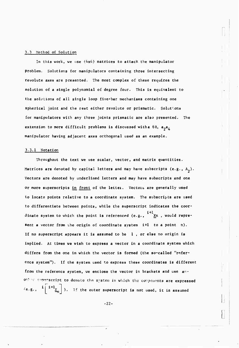
3.3.1 Notation
Throughout the text we use scalar, vector, and matrix quantities.
Matrices are denoted by capital letters and may have subscripts (e.g., A ).
Vectors are denoted by underlined letters and may have subscripts and one
or more superscripts in front of the lettei. Vectoit, are generally used
to locate points relative to a coordinate system. The subscrij-ts are used
to differentiate between points, while the superscript indicates the coor-
i+1 ainate system to which the point Is referenced (e.g., Xn , would repre-
sent a vector from the origin of coordinate system l+l to a point n).
If no superscript appears It Is assumed to be 1 , or else no origin Is
Implied. At times we wish to express a vector In a coordinate system which
differs from the one In which the vector Is formed (the so-called "refer-
ence system"). If the system used to express these coordinates Is different
from the reference system, we enclose the vector In brackets and use ai -
et!- •;■ fripe'script to denote thn system in which the corpoiionts are expressed
'e.g., xl ). If the outer superscript la not used. It is assumed
-22-
'
I
I
I

::
■
to be the same as the inner superscript. Scalar quantities are written
as lower case letters, with or without subscripts (e.g., aisi )• If
they represent coordinates of points, then a superscript is sometimes
used to designate the coordinate system to which they refer. Where no
superscript is used, the number 1 is implied. Angles are denoted by
lower case Greek letters with or without subscripts (e.g., Bi ^ ).
Points are occasionally given a name (e.g., "the point X2 ") and
referred to by name.
The trigonometric functions sin, cos, and tan are abbreviated
s, c, and t respectively (e.g., sin W is written sH, , cos 01,
as cO,. , etc).
3.3.2 Mathematical Preliminaries
In order to analyze the kinematics of a manipulator, we first
establish the relation between two Cartesian coordinate systems as
shown in Figure 3.2. We define the following:
a.: the length of the common normal between z-axis
and z-axis .
i
right-handed sense from z along a line from z
» i+1 to z .
01 : the angle between z and z measured in the
s.: distance from 0. to the common normal a
H.: angle the common normal makes with x-axis.
Then there exists the transformation [46] to express the coordinates of
a point in one system given its coordinates in the other. If we denote
the coordinates in system i by (ix, iy, ^-z) and in system i+1 by
( x, y, z) , we define the vectors ^X and 1 X such that:
-23-

n
and
i+l X =
i+1
i+1
i+1
so Chat the transformation is:
lX - A^h
where
A^ =
c^ -so ca sO.s^ ajcS
SBJ cfi,ca, -c9.sa. a.s6
0
0
sai
o
i"1*! aiaoi
ca.
The inverse also exists and is defined by:
i+1x - A^1 h
where
-1
61 sfi. 0
•sB.ca c^isa1 ^i -s^cai
so sa. -cfl.sa. ca. -s.ca
o o
•24.
(3.1)
(3.2)
I
n i:
I
!,
1.

D i
n
ij
u
For n+1 coordinate systems there are n transformations between
neighboring systems. These may be multiplied, in the following order,
to give the coordinates in the 1 system of any point fixed in the
n+1 system:
— 12 n —
Now to appropriately fix these coordinate systems in a manipulator, we
make 1z correspond to axis i , ^-x to comnon normal ai.i and
define 1y in a right-handed sense. This is shown applied to a sample
manipulator in Figure 3.3. For a six degree-of-freedom manipulator we
write:
lX = A1A2A3A4A5A6 7X (3.3)
where X is a vector to any point, expressed in the ground system
and X is a vector to the same point expressed in a system fixed in
the terminal device. We define
Aeq = A1 ... A6 . (3.4)
With this definition (3.3) becomes:
, 7 X = Aeq 'X (3.5)
and the inverse yields:
7X = Aeq'1 lX (3.6)
Now, if we let P be a vector from the origin of system 1 to the
origin of system 7, and -£ , m , and n , be three unit vectors
aligned with the x, y, z axes respectively, then when ^£ , m , n ,
and P are expressed in system 1, they may be used with equation
(3.5) to find Aeq . That is, using (3.5) we may write
-25-

Figure 3.2. Relation between two coordinate systems.
Figure 3.3. The relationship between coordinate systems fixed in the manipulator.
.26-
I,
i
i:
i
i. i. i:

•
■
:
r -1 _ - — _ _ _, p -. P -i r- - r- -i
1 3
1 0
ml m2
0 1
nl n2
0 0
p3
0 0
= Aeq 0 m = Aeq 0 n3 = Aeq 1 = Aeq 0 0 0 1 0 » 0 0 I 1 1
_ _ _ J 1- —1 L .J i- —1 L- -1 1- -•
from which we may solve for the elements of Aeq to obtain:
Aeq = m
(T (3.7)
It is thus seen that position and orientation of the terminal device
can easily be found, knowing the manipulator variables, 6^ or
s., 1=1,.., 6 , by the matrix product equation (3.4).
However, for computer control of manipulators, the problem is to
find the manipulator variables, given the terminal position and
orientation (Aeq) .
We shall first consider a six-revolute arm and the problem of
finding Ö.,..., 6^ given Afeq. Equation (3.4) represents twelve
scalar equations, nine dealing with orientation and three with position.
However, only three of the orientation equations are independent so that
there are six equations in 8 ,.,,, 8 , These equations have terms of
the form:
cei ce2 cfl3 c64 063 cH6 , (3.8)
sB^ CB2 cfL sH. sÖ,. st)^ , ...
These terms contain both sines and cosines, which we may define in terms
of the tangent of the half-angle.
c9H
1-t -i 2
2
■»j ■ 2t2
l+t2^ (3.9)
•27-

Then if we substitute (3.9) into the six equations, the typical term,
as shown in (3.8) becomes (letting t = tan -^i , i*l,..., 6 , and
removing the denominators which are common):
2 2 2 2 2 2
'l '2 '3 '4 '5 ^ + '••
Thus we see that these equations are quadratic in each of the unknowns
and the degree of the highest degree term is 12.
However, not all the equations contain all of the unknowns and by
judiciously choosing the three orientation equations, the unknowns fl,
and S, can be eliminated froir some of the equations. We use the
six equations:
(3.10)
(3.11)
(3.12,1
(3.13)
(3.14)
(3.15)
which are obtained respectively from the ' 14', '24', 'U', '33', •34',
and '32', elements of the matrix of (3.4). We note that (3.10) (3.14)
do not contain t^ , and (3.13) - (3.15) do not contain t. . Of the
five equations in which the variables t, tc appear at most
quadratica 1 ly, three equations are of degree 10, while, two are of
degree eight. If we eliminate t between (3.10), (3.11), and (3.12),
the result is two equations of at most degree eight in the unknowns
t2»...» tc whose total degree is 32. These together with (3.14) and
(3.15) give us four equations for to,..., t^ . Proceeding in this
-28-
rl (*!.... ' t5) = 0
F2 (tv... ' t5) = 0
F3 (tj.... 1 t5) = 0
F4 (t2,... ' t5) = 0
F5 (4,... , t5) = 0
F6 (t2.... • t6) = 0
I:
;:
1; [

:;
,
manner eliminating one variable at a time, we would finally obtain a
single polynomial of degree 524,288. Even though this method of
elimination introduces extraneous roots, we would still expect, according
to Bezouts' theorem*, (10) x (8) or 64,000 common roots, a number much
too large to cope with. The general problem, attacked in this manner,
is insoluble. At this point we shall define a "soluble case" to be one
in which the degree of the final eliminant is low enough to find all
roots. In practice all the roots of an eighth degree polynomial can be
found within a few seconds using a digital computer and the roots of a
fourth degree within one-half second. A solution is said to be
"closed-form" if the unknowns can be solved for symbolically.
Even though the general problem is beyond reach, many practical
manipulator configurations are soluble. The existence of three revolute
axes intersecting at a point leads to a soluble class. In the next
sections we explore the possible combinations of three intersecting axes.
3.3.3. Last Three Axes Intersecting
If the last three joints are revolutes and their exes intersect
as in Figure 3.4, then their point of intersection, as designated by the
vector P-j is only a function of motion in the first three joints and
the constant link parameters. P- is known by specifying the hand
position and orientation. We want to solve the three scalar equations
represented by:
^3 rt 1 rt r\t\ *}
0 0
•i 1
(3.16)
♦Bezouts' theorem gives an upper bound to the number of common solutions for a set of equations. The upper bound is the product of the total degrees of all the equations.
-29-

n ;
o D I: :
D D
Figure 3.4, The most general manipulator having the last three revolute axes Intersecting.
-30-
i,
i:
i.

i
;
:;
o i! D •;
:
fi
D
0 0 ;.
D D Ü
D
for the variables associated with the first three joints. We now derive
an Important result used In the solution of this problem. We define
(3.17)
where A* (i ■!»••.» J) Is defined In equation (3.1). It Is seen
that Pj Is a vector specifying the position of a point (0, 0, s. ,)
which Is fixed In coordinate system j+1 .
We may write (3.17) as
the vector -PJ 0 0
^j = Al ' •AJ sj+l
1
Pj « (A1A2) A3 ... A J+1
A1A2
V*} flj)
f2(83...., flj) (3.18)
where
J+1
(3.19)
Then using (3.1) for Ai and A2 (3.18) becomes
ce1g1 + se1g2
h 8ei«i •182
^8a1[sQ2(a2 + fp - ce2(-ca2f2 + sajfs)^
+ ca1(9a2f2 + ca2f3 + s2) + ■!
l
(3.20)
-31-

:
■
•
where
gl = cö2(a2+f1) + se2(-ca2f2 + sa2f3) + al (3.21)
g2 ■ -se2ca1(a2+f1) + c^2cal(-ca2f2 + sa2f3)
+ s'i1(sa2f2 + ca2f3 + s2) . (3.22)
Denoting the components of P* by x. , y. , z. , v; define
Rj = x5 + yj + (zj"s])2 • (3-23)
With (3.20) for the components of (?.) , (3.23) becomes
Rj = l^ + f22 + f3
2 + a^ + a22 + s2
2 + 2a2f1
+ 2s2(sa2f2 + ca^fj) + 2a1L c?2(a2',"f P
+ sp2(-ca2f2 + sa2f3)] (3.24)
We note from (3.20) and (3-24), that we may write:
R] = (F1ce2 + F2sp2)2a1 + F3 (3.25)
zj = (F1«e2 - F2cy2)sa1 + F4 (3.26)
where,
I Fl a a2 + fl (3.27)
F2 =-ca2f2 + sa2f3 (3.28)
F3 = f^ + f22 + f3
2 + aj2 + s22 + 2a2f1 + a2
+ 2s2(sa2f2 + ca2f3) (3.29)
F4 = ca1(sa2f2 + ca2f3+s2) (3.30)
Equations (3.25) and (3 26) prove to be very useful as Ö, has
been eliminated, and 42 appears in a very simple form.
Returning to the manipulator problem, the above equations
apply with j = 3. In which case by using (3.1) for A- (3.19) jT]
becomes:
0
0
1:

\
w
■
;,
ü ü Q
Ö
'fl
f2 m
h_
s4s938a3+a c93
-S4ce38a3+a3s93
84crt3+83
(3.31)
so that with (3.21), (3.22), and (3.31) equation (3.20) represents
three equations in three unknowns. If the first three joints
are prismatic, then (3.20) represents three linear equations and
is easily solved. The othe^ possibilities are somewhat more
difficult, but may be solved as follows:
3 Revolute - ^l,_^2»—3 all variable
Substituting (3.31) in (3.27) - (3.30) yields respectively
Fl = a2+8, S03sa'i+a3c93
1+ tan j
2
•33-
(3.32)
(3.33) ^2 =-ca2("8Ace3sr,3"w38e3) + 8rt2^83+84crt3^ 2 5 2 2 2 2
F3 = a^ +8- +82 +s3 +a3 +s. +2s283ca2+2s2S,002013
+ 283s4ccx3+ce3(2a2a3-2s2S48a28a3) + 893(28382802
+ 2a2848a3) (3.34)
F4 = CQ,, |.a3893sa2+s3ca2+82+84("ce38a2sa3',"ca2c£I3^ (3.35)
Now we note that the left hand nide of (3.25) and (3.26) are
known and that if a^ = 0 , (3.25) reduces to
R3 " F3 (3.36)
When (3.34) is used in (3.36) it is simply a function of 93 .
Then making the additional substitution
1-tan2 93 c9, = L (3-37)

2 tan 63
se^ = I (3.38) J 1 + tan 83
2
•34-
0 into (3.36), yields a quadratic in tan 9-> . Similar simplifi-
cation results if snrj=0 , as (3.26) reduces to a quadratic. If
however sc.i and a, are non-zero, we eliminate 8^2 and c^j
from (3.25) and (3.26) to obtain the polynomial
D (R3 - F3)2 («- F4)2 2 2
— + ^— ■ F^ + F2 (3.39) 2a! sn-^
Upon making the tan 93 substitution and using (3.27) - (3.30) equation 2
(3.39) is of degree four in tan 93 . After getting 93 , 92 7
may be obtained from (3.25) or (3.26) and 9i from (3.20).
!:
^l»_®ii—§3 variable
Here we take the x and y components of P3 as defined
in (3.20)
x = c91g1 + s91g2 (3.40)
y = s91g1 - cQjgj (3.41)
Solving for g^ and g2 we find
gl = XC9! + ys91 (3.42)
g2 = -yc91 + xsQ] (3.43)
so that g^ and g2 can be computed from x3.42) and (3.43).
Then examining (3.2i) and (3.22) using (3.31) we note
g! = c92h1(93) + s92h2(93) + a^^ (3.44)
g2 = ca1[c92h2(93) - s92h1(93)] + sn,^^) (3.45) 1 •
L i:

where
h, = 3^89330.3+83003 (3.46)
h2 " sA(ce3ctt2srr3+sa28a3) " 83803^02+s3sa2 (3.47)
^3 " 84(-c038a2a^3+ca2ca3) + a38e38a2
+ 83002 + 82 (3-^8)
If cai = 0 then (3.45) is easily solved for 93 . If
co. ^ 0 we eliminate 02 from (3.44) and 0.45) to get the
i;
polynomial
2 2 2 hi + h2Z - (8,-«!)
L. örr,!
Expressing 803 and c9, in terms of tan 93 leads to a J 7
polynomial of degree four. Upon obtaining the four roots of
(3.49) we substitute into (3.44) and (3.45) to get 92 and
finally (3.20) for Sj^ .
Q\t 89, 9^ variable
Solve (3.26) for 82 , using this in (3.25) results in a
fourth degree polynomial in tan 93 . Then proceed as in all
revolute case.
[I 9^, 02, S3 variable
Similar to 9^9293 variable with the exception of s-
being the variable in the final polynomial which is of degree
II four.
(3.49)
lLS2^3 var^ahle
The left-hand side of (3.44) may be computed from (3.42), then
(3.44) which is quadratic may be solved for 93 . Finally s^ and S2
may be found from (3.20). -35-

1L§2^3 variable
It Is possible to eliminate 02 as in the case of s^öß
variable, resulting in a quadratic in s- .
i*ll2ih variable
Equation (3.25) is solved for 82 and used in (3.26) resulting
in a quadratic in S3 , 0^ is found as in the all revolute case.
Methods have been presented to find the first three variables.
At this time we leave the problem of finding the Ifst three angles to
be dealt with later in this work (see Section 3.3.6).
3.3.4 First Three Axes Intersecting
Next consider the three intersecting axes to be the first
three, as in Figure 3.5. The solution of these is analogous to
the previous exair~le. We define a vector ^P from the hand to
the point of intersection of the three axes, as shown in Figure 3.5.
We note that when 'P is expressed in a coordinate system fixed
in the hand, that it is just a function of the last three joints.
That is:
7P = A, 1 -1 -1
0 0 0 1
(3.50)
To Usiag (3.2) for A3' and forming A3 0
LLI we get
7P - A^Aj'V1 -a3 -S3sa3 "s3ca3
1
(3.51)
If we use (3.2) to express Ag , A5 , and A4 then the
right-hand side of.(3.51) just contains the three variables associated
-36-
:
D I. 1.

.
i
;
with the last three joints. In addition, we compute the components
of 'P from
7P = Aeq ■1
where Aeq is the known matrix (3.7). We note that the rotation
portion of Aeq is just the transpose of the rotation portion
of Aeq . In fact, if
Aeq =
all a12 a13 ai4
a21 ä22 a23 a24
a31 a32 a33 a34
(3.52)
then
Aeq -1
all a21 a31 al4
a12 a22 a32 a24
a13 a23 a33 a34
0 0 0 1
-1
-1 (3.53)
The elements denoted as a^' , a2-" , 834" are determined by
simply applying
thus
Aeq"^ Aeq ■ I
-1 (3.54) ai4 = -(alia14 + a2ia24 + a3ia34)
1=1,2,3
From this point on the method of solution follows the same steps given
in Section 3.3.3 for the case of the last three axes intersecting.
.
-37-

::
[ i: :
■
i
Figure 3.5. General Manipulator in which the First Three Revolute Axes Intersect at a Point.
-38- L [
!
::
D
;
n
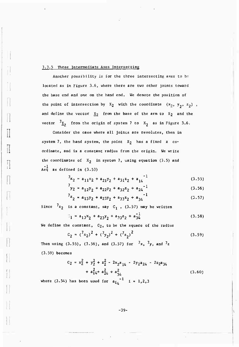
3.3.5 Three Intermediate Axes Intersecting
Another possibility is for the three intersecting axes to hr.
located as in Figure 3.6, where there are two other joints toward
the base end and one on the hand end. We denote the position of
the point of intersection by X2 with the coordinate (x,, y , Z2)
and define the vector X2 from the base of the arm to X2 and the
vector 'Y« from the origin of system 7 to X2 as in Figure 3.6.
Consider the case where all joints are revolutes, then in
system 7, the hand system, the point X2 has a fixed z co-
ordinate, and is a constant radius from the origin. We write
the coordinates of X2 in system 7, using equation (3.5) and
Aeq as defined in (3.53)
(3.59) becomes
c2 = x2 + y2 + z2 " 2x2aI4 " 2y2a24 * 2z2a34
+ af4+ a^ + a^ (3.60)
where (3.54) has been used for a^ " i = 1,2,3
7x2 = allx2 + a2iy2 + a3lz2 + ai4*1 <3-55) 7 , ^2 = al2y2 + a22y2 + a32z2 + a24 (3.56)
7z2 = a13y2 + a23y2 + a33z2 + a34 (3.57)
Since '22 is a constant, say C^ , (3.57) may be written
1 = a13x2 + a23y2 + a33z2 + a34 (3.58)
We define the constant, C2, to be the square of the radius
C2 = (7x2)2 + (7y2)2 + (7z2)2 (3.59)
Then using (3.55), (3.56), and (3.57) for 7x, 7y, and 7Z
-39-

s, x2 (x^y2.23)
•
j
Figure 3.6. Manipulator with three Intermediate revolute axes Inter- secting ( I.e. a =s =a =0 ).
3 4 4
-40- !.
1.

n :
:
::
;
h
With j = 2 (3.20 becomes
[a2(ce1c92-s01s02ca1) + S2s9 sa.+ajcQj + s (00 se2sa2 +
89^92^250,2+89^^2)]
[32(89^92+091892001) - 8209,80]^ + a^i
+ S3 (89289280.2-09^92001sa2-09^2002)]
[32892802 + 82002 + 82 + 83 (-092802802+002002^
1
snd (3.27) - (3.30) become
Fl =a2
F0 = 83SO2
F3 = 31+8^+3^+82+2328.002
F4 - •3ca1ca2+t2
So thst using (3.62) - (3.65) snd (3.23), equstion (3.39) becomes
(3.61)
(3.62)
(3.63)
(3.64)
(3.65)
.2222222. , ^X2 y2 2"al'S2"a2'S3 2S3ca2^
23.
Z2-S3C0 2c<l2"s2
so 1
2 2 2 ■ 82+8-802 (3.66)
Then (3.58), (3.60) 3nd (3.66) 3re three equstions for the unknowns
(x2y2Z2). Ordinsrily the system would result in 3n eighth degree eliminant
but since (3.60) 3nd (Ö.66) may be combined to form
~,r ^ ^ ^ 2 2 2,2222- (C2+2x2a14+2y2a2^-Z2a34-al4"a24-a34)-arS2"a2-S3-2s2S3Ca2
2a I
Z2*S3calca2"S2
so. 32 + S3SO2 (3.67)
-41-

The equations (3.58) (3.60) and (3.67) may be combined to yield
a single fourth degree polynomial In one variable, say z ,
After the values of z are determined It Is possible to back
substitute and obtain corresponding values for x and y .
Once the coordinates (X2, y2, Z2) of the point X» are
found, 92 and 9 may readily be found from equation (3.61).
9^ Is easily evolved by noting:
7..
'72
7«2 ^2
-1
•a5
•858a5
•s5ca5
Using (3.2) for Ag , with a, = s^ » 0 , (3.68) becomes;
12
.a5c96 85896
(3.68)
(3.69) a5896ca6 + 85(-c968a5ca6-ca59a6)
-a5s96sag + S5(c9g8a59a6-ca5ca6)
l
Since x2, y2 and Z2 are known (3.55)^3.56) and (3.57) may be
used to calculate ^^2' Then (3.69) may be solved for 9g . The
problem of solving for 9^ 94 95 will again be deferred (see
Section 3.3.6).
The preceding solution was for all revolute Joints. We now
consider the cases in which Joints 1, 2, and 6 may be prismatic.
lL§2§6 variable
Eliminating s 92 and c92 between the x- and y- components
of (3.61) results In a quadratic in X2 and y2 . Then this equation along
-42-
11 0 i,
\
D i: D
i:
i: ■
i. [ L i

]
I D D i: i
s D !!
D D
22
c + b t , (3.70)
where b is a unit vector parallel to this line and c is any fixed
point on the line. Eliminating t , yields two equations between
x2 » y2 » and z2 • Th60 with these in place of (3.58) and (3.60),
the procedure is the same as previously indicated.
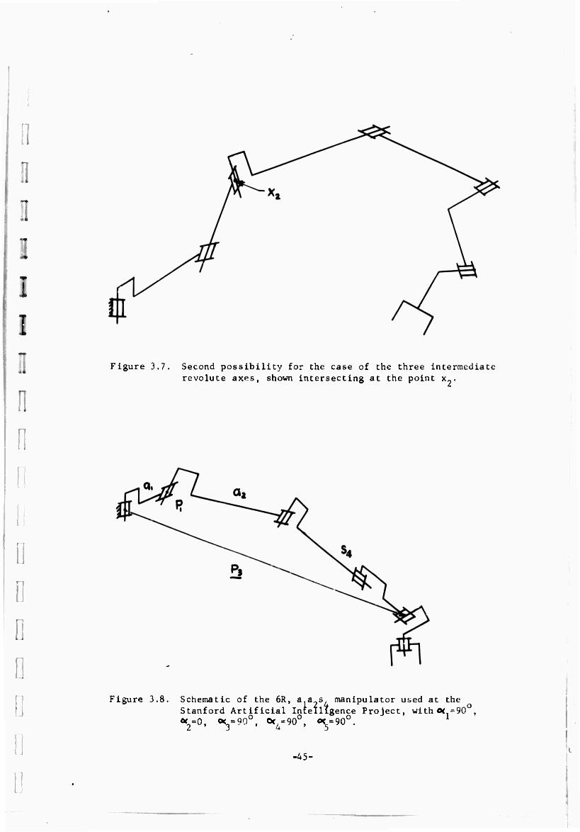
The second possibility for three intermediate axes to intersect
is as shown in Figure 3.7. This is just an inversion of the case
treated in this section and may be solved in a similar manner.
-43-
with (3»58) and (3.60) can be reduced to a single fourth degree poly-
nomial in either x« or y2 .
®ll2—6 variable
Forming (3.25) and (3.26) with j = 2 aud then eliminating S2
between them, a fourth degree equation results in a manner similar
to the all revolute case.
1LS2^6 variable
First 32 may be eliminated between the x- and y- components
of (3.61). The resultant is a linear equation which along with (3.58)
and (3.60) can be combined to form a single quadratic.
If St is variable instead of 0 , equations (3.58) and (3.60) 0 6
no longer apply. However, the point X2 must lie on a known line.
This line, in the direction of axis 5 may easily be found, and may be
written in terms of two known constant vectors c and b and the
parameter t as:
"x2"

3.3.6 Completing the Solution
It can be seen from the foregoing that if three adjacent revolute
axes intersect at a point, then the solution to the problem can be
reduced to a single equation of degree four. If, in addition, two of
the remaining three joints are prismatic, the problem redv;es to a
quadratic.
Simplification will also result, if special geometry exist in
additinn to the three intersecting revolute axes. Consider the all
revolute case, with only a^ , a2 , and s, non-zero and
04 = 90°, (12 = 0 , 013 = 90°, a4 = 90°, a5 = 90°, as shown in
Figura 3.8. This is the configuration used for the hydraulic arm at
the Stanford Artificial Intelligence Project. With the above values,
equation (3.17) becomes
a^Q^ + a2c91ce2 + s, (c01ce2s93+c91s92c93)
als9l + a2seice2 + S,t(s91c92s93+s91s92c93) ( J . 7 1) h a2S02 + S4(s92s9 -cri2c9 )
_ 1 and (3.27), (3.28), (3.29), and (3.30) become
Fl = a2+s, s9-j
E2 - s4c93
F3 = 2a2S S93 + s^2 + a-2 + aj2
F4 = 0
So that equation (3.25) becomes:
R3 = s42 + a22 + al2 + 2a2S4s93 + 2a1a2c92 + 2a184(c92s93
+S92C93)
(3.72)
(3.73)
(3.74)
(3.75)
.
ii
y
(3./6) II
.44. 1 1.
:
:
:
:
i i
::
a
D
Figure 3.7. Second possibility for the case of the three intermediate revolute axes, shown intersecting at the point x .
Figure 3.8. Schematic of the 6R, aas manipulator used at the Stanford Artificial Intelligence Project, with o< =90°, <*2=0, <X3=90
O, Ot4=90O, 0^=90°.
-45-
.

and (3.39) becomes:
R.3-(2a284893+842+a2
2+a12)
—, 2
+ z2 = (a2+84893)2 + 84
2ce32 (3.77)
which ia quadratic in 80- when cQ-f is replaced by 1-89 .
After finding %^ we compute $2 froin (3«71) and (3.76) and 9,
from (3.71).
Since the above arm is useo in the Stanford Artificial Intelligence
Project, we shall use it to illustrate the method of finding the angles
associated with the three intersecting axes. Designating the direction
en of the lüi axis by the unit vector y^ , we write
«ft " A1A2A3A4 (3.78)
Using (3.1) for A^,..., A, and the above values of a the
result is
c9^c92s92 + c9js92c9o
^ ■ 89ic92s93 + 8e1s92c93 (3.79)
s92s9ß - c92c9-j
0 _
so that 0)4 may be computed from (3.79) as we have solved for 9^ ,
82 , and 03 • igg is known since the hand orientation is specified.
In addition,
MJ4 . jfij - co8a4 (3.80)
iK5 • JJ16 " cosa5 (3.81)
MS • JK s ^ (3.82)
-46-
D :'
D !:
0 D f D i
Ö
L
i;
1:
i:
i:

1 :l D 0 D
i
i
i! D ll 0 II li I! D Ü
where n, and de are link parameters of the arm. In fact 4 5
a^ -90° and ou ■ 90° . We can find the components of 015 by
simultaneously solving (3.80), (3.81) and (3.82). We observe
7r«..1 - A,"^ "1 ^5]
0 0 1 0
(3.83)
using (3.53) for A6 and A5 with a4 - ttj - 90° and a6
(3.83) becomes:
'"sG<
7 Ctt.]
ce(
0
0
(3.84)
and
7[(j!5] = Aeq" mj (3.85)
where Aeq is the known matrix specifying hand position and
orientation equation (3.7). Its inverse is found as in Section 3.3.4.
So that we easily derive 9, by equating the right-hand sides (3.84)
and (3.85). We also write
w = \ A5 Vl
0 s95c96
0 X
-s95s96
1 -c95
0 0
(3.86)
and
[^] - Aeq jij (3.87)
■47-

J
which yield 9, . To obtain 9. we proceed similarly
7ü«3] - \ vV1^"1
0 sG.cG-cG, - 4 5 6 C04806~|
0 -80.cQ 80, 4 5 6 - ce4ce6
1 804805
0 0 —1 L_ _J
(3.88)
and
7[UJ3] - Aeq"1 ^ (3.89)
which yields 0,.
We have indicated a procedure to find the rotation about three inter-
secting revolute axes when these are located at the hand. The method
is applicable when any three axes Intersect. However, the equations
must then be rewritten in terms of the Wj_ and 0^ associated with
these axes.
3.3.7 Solution for Any Three Joints Prismatic
A six degree-of-freedom manipulator with any combination of three
revolute and three prismatic Joints is soluble. This arises from the
fact that, the orientation of the hand is Independent of the displacement
in the prismatic Joints, and is only a function of rotation in the three
revjlute Joints. In addition the orientation is independent of the
position in space of the revolute axes. Consider the manipulator shown
schematically in Figure 3.9. The direction of the first revolute axis
is always fixed. With the hand orientation specified, the direction of
the third revolute axis becomes fixed. In addition we know the angles
which the axis of the second makes with the axes of the first and third
revolutes. If we designate the direction of these revolute axes by the
-48-
Q
Q
11 D II
i,
11 !:
I D I. !!
1: i; I! E E I

D Q
[1
I]
[1
unit vectors, Uh ' ^3 » and ^5 tlien we ,nay write
12 • J|3 ■ cosBj (3.90)
■3 • IS ■ C08ß2 (3.91)
«3 • % - 1 (3.92)
where Bi and B7 are the known angles. The equations (3.90)
(3.91), (3.92) are then solved for the components of cy^ . The
Joint angles may be found in a manner analogous Zo that used in
the previous example, as the now known direction UJ. • can be
expressed only as a function of O2 which leads to a simple
equation for 9» . ^- can also be written in terms of 9 alone,
yielding 9, . Once 92 and 9c are known, 9. is easily found
by rewriting (3.4) as
A3 " A2" Al Ae<lA6 A5' A4
l\
ll
D il
D
il
11
0
Using the values we found for 9? and 9 plus the constant angles,
we compute the rotation portion of the right-hand side of the above
equation. Then writing A-, as in (3.1), we may solve for c9j and
s9~ , thus finding 9- . The displacements in the prismatic Joints may
be found from (3.4). Since all the angles are now known and the s's
only appear linearly, the displacement portion of (3.4) easily yield
these three unknowns s^ , s, , and s .
3.3.8 More Difficult Arrangements
In the previous examples, the existence of three intersecting
revolute axes enabled us to separate the problem into two parts -
one dealing with position and the other with orientation. The two
problems were chen solved separately. That is we solved a three
-49-

degiee-of-freedom position problem and then a three degree-of-freedom
orientation problem. A more difficult problem is one in which potiltion
and orientation do not separate. An example is the case where Just two
revolute axes intersect. Consider the 6R , a,S2*2B'iBiiaLa5a5 man''"
pulator shown in Figure 3.10. Here axes 3 and 4 Intersect. The vectors
7P i S i and R are a& shown in Figure 3.10. We make the following
observations:
Q - A1A2
^-VS"
0 0 s3 1
-a4
UJ3 - A ^2
0 0 1 0
7Ca.4] 0
A'lA lA -1 0 6 5 4 1
0 J lr7 c'p] - a - R
Then using (3.1) for the A's (3.93) - (3.96) become (taking
«! - s6 - a6 - 0) :
-50-
(3.93)
(3.94)
(3.95)
(3.96) 11
(3.97) Li
- 2^ . R (3.98) 0 ome (taking 0
0

~m.m
D D II ii
D !l
D Q
D il D 11 ii II ii Si Q
Q
Figure 3.9. A general P-2R-P-R-P manipulator.
Figure 3.10. A 6R.ai82a28384a4S5a5 nuinlPulator- Axe8 of Joint8
3 and 4 Intersect.
-51-

7P =
S3(c91s92sa2+s91ce2ca1sa2+s61sa1ca2)
s3(8e1se2sa2-ce1ce2c318a2 - c91sa.1ca2)
+a2(se1c92+ce1892ca1) - 82ce1sa1 + a1s91
s3(-c9 sa1sa2+ca1ca2) + a2s92sa1 + 82ca1
l
a4(-c95c96+s95896ca5) - a5c96 •• s58968a5
+84(-895c96sa4 - c95s96sa4ca5-s9bQi48a5)
a4(c95s96+895c9,cac) + acS9, - s c9,sa.5
+84(s95s96sa4-c95c96so4ca5 - c96ca4sa3)
-a4895sn5 + su(cQ5saUar'5'Ca^ca5^ ' s5ca5
■3
7[^J
c9 s928o,2 + 891c92ca18a2 + 89 sa1ca2
s918928a2 - c91c92ca1sa2 - c918a1ca2
-c928ai9a2 + caica2
895c963n4 ♦ C95s96sa4ca5 + 89(>c^8rl5
-s95896sot4 + c95c968rt4ca5 + c96co4sa3
-c95sa48a5 + ca4ca5
0
52-
(3.99)
(3.100)
(3.101)
(3.102)
I:
W
n n l!
I:
I
I
L L

___. —.
.1
0 rl
D D 0 D D D
D
Ö
li
D 'I
I :!
In addition (3.99) and (3.100) respectively yield
2 - 83 + ^2 + 82z + a^ + 2a1a2C02 + 2ai838a28e2 + 23283002 (3.103)
7Z2 ■ a42 + 852 + as2 + 842 + 2a4a5ce5 + 294a5s, S^A + 284850014 (3.104)
Our approach to this problem is to solve for the coordinates (x, y, z) of
the point of intersection of axes 3 and 4. With this in mind we
eliminate 82 between (3.99) and (3.103) which yields the polynomial:
2 I 2 _ ,„.2^. 2^,_2J- 2. (SßS-a? +82 4a, -^s^s-^CGp)
2a,
1— —2 z - S2cai - 83ca1ca2
L ^i _ 2, 22
a2 + 83 ■a2
where we have defined 2 ^n terms of its components
and
y z
Q2 - x2 + y2 + z2
Similarly eliminating 85 between the z-component of (3.99) and
(3.103) leads to
[- Z2 - (a42+8c
2+a «5^4^848^004)]' 2a5 J
—, 2 2+84004005+85005
so.
2 2 J 84''804 + 84
We note ^p] ^C^] - 7P . 7P and using (3.98) for ^V)'
we form
7p2 . 22 + R2 - 22 . R
-53-
(3.105)
(3.106)
(3.107)
(3.108)
(3.109)
-1 -.
ilso
Aeq -1 y
z
1
(3.110)
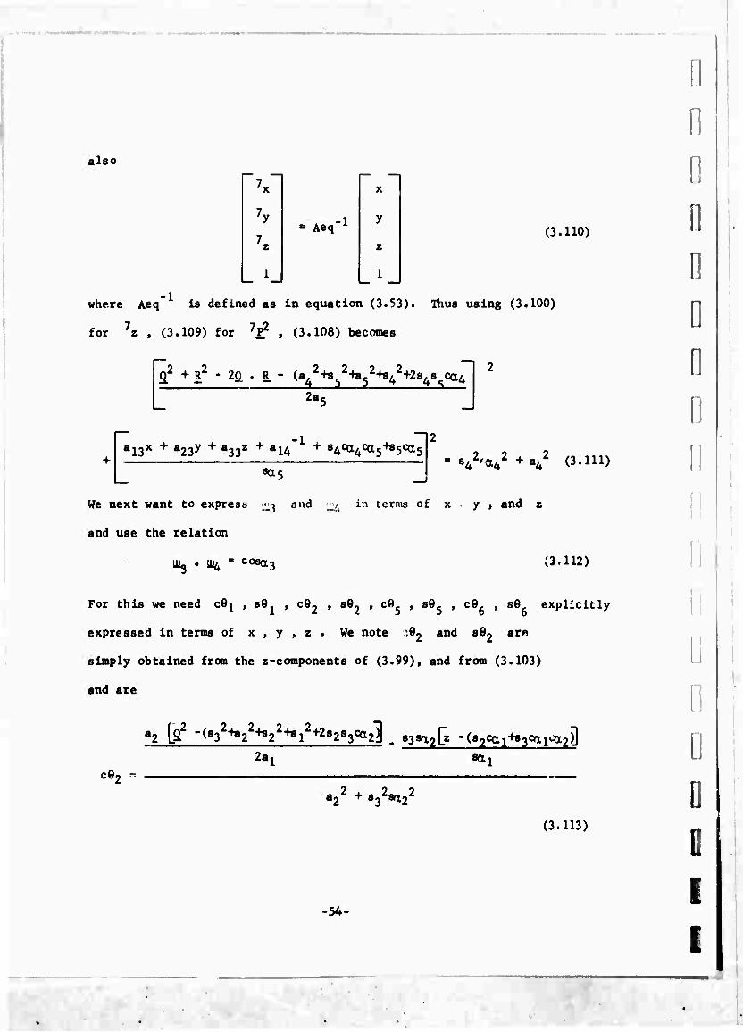
where Aeq Is defined as In equation (3*S3)a 'flius using (3.100)
for 7z , (3.109) for V , (3.108) becomes
22 + R2 - 2ß . R - (a42-^5
2-^52-ts4
2^2s48[.ca4
2a.;
i13x + 8237 + a33z + a14~ + 8^ca^ca5+B5ca5
sa5
842'a42 +a4
2 (3.111)
We next want to express ^3 and IJV in terms of x y , and z
and use the relation
Uj • t^ ■ cosa3 (3.112)
For this we need cOj , 80 , 082 , sO- , eft , sft, , c9 , sft explicitly
expressed in terms of x , y , z . We note ^ and S82 ar^
simply obtained fron the z-components of (3.99), and from (3.103)
and are
a2 [22 -(S32 W-fa^283^231 ^ ^^ -(82ca1-f33ca1^2)]
2a, ^1
eft, -
»22 + 8328a22
(3.113)
•5A-
i! !!
I! il i:
f:
I- I
I
i,
D 0 I I

D 11
il
D f! D D
D D D D Q
ii
e2[z -(82ca1-^3ca1ca.?j » 83sa2 1^ ~(s:i2+azZ-hi2
2+a12+282s3c(l2')\ sai 2a! L J
80, " a2 + 832sa22
(3.114)
c9i and sflj from (3.99) are, after simplification
m x(838e28a2+a2ce2+al) ' ' [s3(ce2Calsc2+8alC;a2^ " a2B92c^i + s28ai]
x2 + y2
(3.115)
y(83s928a2+a2ce2'fal^+ x[f3(ce2caiaa2'f8alca2^ " a2s02c^l + s2s'llJ 39,
x2 + y2
(3.116)
Where we may use (3.113) and (3.114) for 082 and se2 . When (3.113)
(3.114), (3.115) and (3.116) are used in (3.101) to express ^3 m
terms of x , y , and z . the result is a third degree expression in
x , y , and z . If we do similar things with Ü5 and 9^ lot ^
then (3.112) becomes a polynomial of degree six In x , y , z . Tliis
along with (3.103) and (3.111) are three equations for x , y j and
z . However, they are of such large degree that finding all the roots
is not feasible. Though there are some special cases of interest.
For a 6R ( 8284 manipulator, with a^ " (13 s ttt " 90° and
012 Ä (14 = -90° the equations reduce to a degree which is workable.
This configuration is shown in Figure 3.11. Equation (3.105) reduces
to
x2 + y2 + z2 - a22 (3.117)
and (3.111) reduces to
x2 + y2 + z2 + x42 + y4
2 + z42 - 2xx4 - 2yy4 - 2z4z - a4
2 (3.118)
-55-

Figure 3.11. A oR,a a. manipulator with adjacent axes orthogonal. X (x,y,z) is the point of intersection of axes 3 and 4.
•56-
i.
[ o D D ;:
r
i:
!:
i.
I.
i. L
L
••
D D D
D D :1 11 D D D D D Q
U
D D
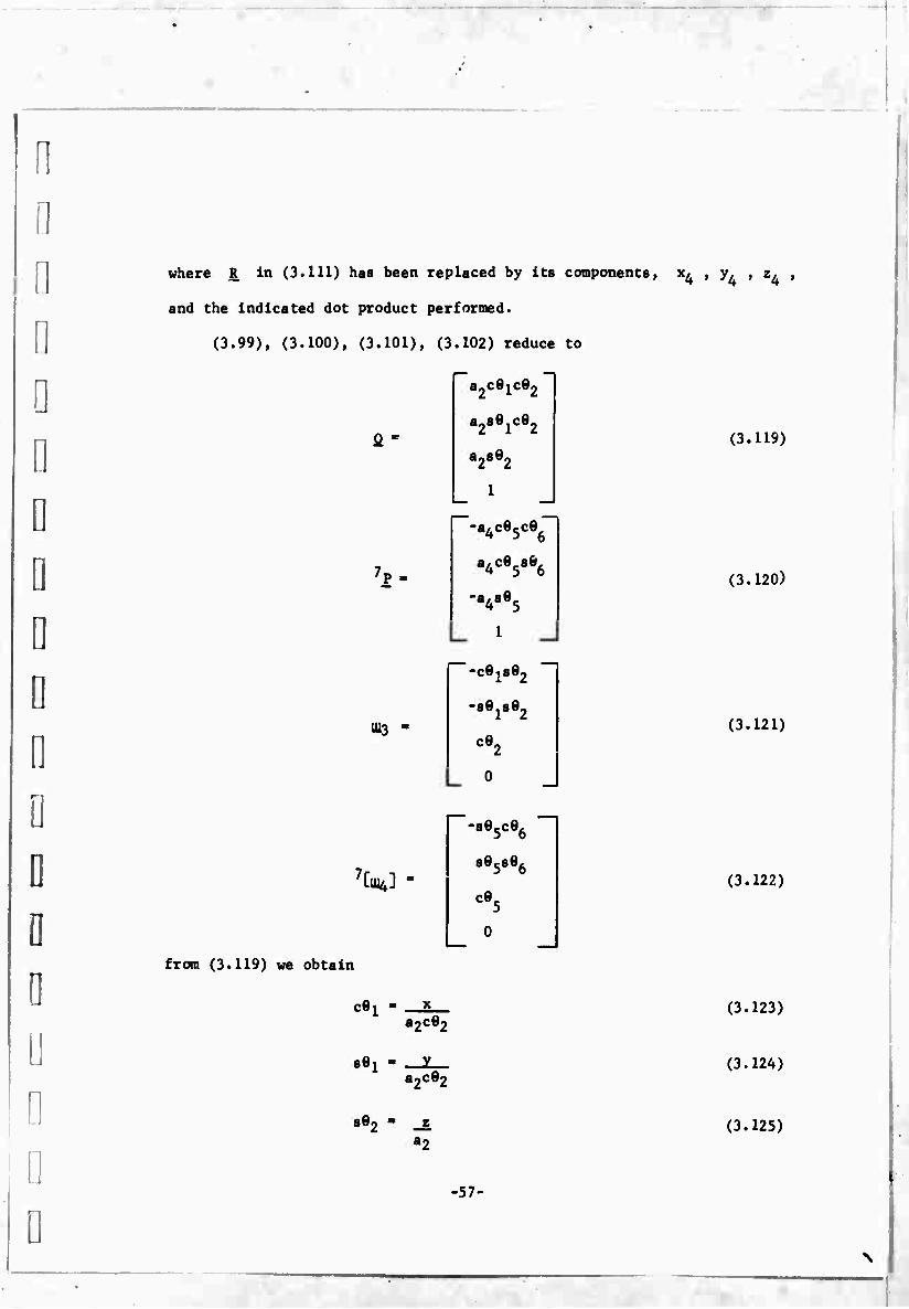
where R in (3.111) has been replaced by its components, x4 » YA i z,
and the indicated dot product performed.
(3.99), (3.100), (3.101), (3.102) reduce to
7p-
1Ü3
V] -
a2ce1ce2
a289lce2
82882
"-a4ce5ce-
a4ce58e6
-a48e5
1
■-ce18e2
-8e1se2
ce.
■se5ce6
sOjsOg
cO^
from (3.119) we obtain
c«l m X
82082
■•l ■ v a2c92
802 « z a2
-57-
(3.119)
(3.120)
(3.121)
(3.122)
(3.123)
(3.124)
(3.125)

■
using (3.123), (3.124), (3.125) in (3.121)
^3 n •2Zc92
•xy
•yz
HW (3.126)
replacing cfy by 1 - 882 and using 8e2 from (3.125), (3.126)
becomes
1113
from (3.120) we obtain
RT
-xz
•yz
■z2+a22
(3.127)
c«6 " 84085
8e6- 84083
se5- -7z a4
(3.128)
(3.129)
(3.130)
substituting (3.128), (3.129), and (3.130) in (3.122) and simplifying
gives U3
7 CUI4] -m*
.7 7 y z
-v, z +a/.
(3.131)
•58-
ii
r. l! 0 D n D i: I" 1
1
I:
I.
1; 1; [

i
ii
D Q
D il D Ii ii D D ;;
D D D D D Q
We now rotate [ml to express it in terms of system 1 by
1U4 * Aeq Qi^]
with Aeq as in (3.53) and 7[u^] as in (3.131) we get
•B117X7Z - a12
7y7z - a137z2 + a^a^
"a2l ~ a22 ' z " a23 z + a23a4
(3.132)
IU4 rxn? 1 - z a4
V 7 7 7 7 2 2 -anj/x z - 832 y z - aßß z + a33a.
(3.133)
To eliminate 7x , 7y , 7x from (3.133) we use (3.110) with Aeq from
(3.53) which after simplification yield:
-(a13x4a23yfB33Z+a3/| ) (x-x4) + ajja^
-(a13x-fa23yfB33z4a34"1)(y-y4) +8238^ ^3 134)
-(a13x+a23y-^B33Z+a34"1)(z-z4) + a33a42
0
** *h'
Then using (3.127) for ^3 and (3.134) for ^ the equation
1Ü3 * iü4 * ^ results in the polynomial:
z(a13X+a23r+a33Z-^34" ) (x2+y2-f^2_XX4_yy^-zz^.a2 -^^2)
-12. 2/ ^ ^ ^ "U 2 2 + za34 a4 + z4a2-c(ai3X-ha23y+a33z+a34 ) + «2 a4 a'
(3 135)
•2 a4 a33
We note that linear combinations of the equations (3.117), (3.118) and
(3.135) can be formed to reduce the degree of the equations.
Equation (3.117) we leave as is. Combining (3.117) with (3.118)
leads to
2x4x + 2y4y +i4z + a42 - a^ - (x^^2^2) - 0 (3.136)
and using (3.136) and (3.11/) in (3.135) yields
■59-

o = «c^Ä-. x42 + yu + H1 . f^)i 2 2
13 , a22 ^2 + y42 + z42 a42 vT ZJ 2 2 2
+ y,[«,,<- a±- .
+ z2[ao,( 33v 2 x^2 + y^2 + Z42 ^2 1
+ x (a13z4a2 ^
23Z4a2' + y (a-.z.a,2)
-1- 2 a2 . ^4 •>• y4 1 z4 . a4
(3.137)
az2 + Z [(«33z4a2'> ■f«34'W fa34 < 2
2-1^22 + z4a2 a34 + 82 a4 a33
The equations (3.117), (3.136) and (3.137) are three equations for
x , y , and z . The linear equation (3.117) can be used to eliminate
one variable easily. Another variable can be eliminated between (3.136)
and (3.137) leading to a polynomial of degree four. This procedure
has been carried out and programmed on the PDP-6. An analysis program
was used to generate inputs with known angles to check the results.
A typical example was generated by the arbitrary input angles
%l - 34° , 92 - 21° , 93 - 780 , e^ -_56o > e5 . 230 , 96 - 1° and
link parameters a2 " a. ■ 15" , which gave:
)]
Aeq
-0.322 -0.481 0.816 12.066
0.555 0.641 0.577 18.035
-0.801 0.598 0.037 -5 609
0 0 0 I
-60-
i;
I,
i: 1: 1
1: 1 !
I D L
L
[
[
L [

i
D i\
D il Ö
n D i;
D !:
D i:
il
D
For the above, the four sets of common roots were real and lead to
four sets of angles for each root. They are shown in Table 3.1.
If aitO then the solution may first be expressed as three
quadratic equations in three unknowns (x , y , and z) and finally
as an eighth degree polynomial. With aj^O , a^^O , a^0 » and a's
as before, and with x , y , z defined as before, (3.105) becomes
(x2 + y2 + z2 . ai2 . 322)2 + 4ai2 (z2 . ^2) = 0 (3.138)
and equation (3.111) reduces to (3.118) as previously noted. To
form UQ we use cOj and s9 from (3.115) and (3.116). Next
we use cQ. and se2 from (3.113) and (3.114) and substituting
these quantities into (3.101), we obtain after simplification:
||U
U2^i*n (x2ty2^2~a22-a1
2)]
- 2xz
- 2yz
- 2z2 + (x2-fy2+z2-a22) + 2a^2 . ^2
0 (3.139)
U^ is as beiore and given in (3.134). By using (3.139) and (3.138)
in (3.112)$ by replacing (x2+y2+7.2) with its equivalent from (3.118),
and by simplifying, (3.1J2) becomes:
0 = x2(2a13Z4x4)
+ y2(2a23z4y4)
+ z2[a33(-R2-a42+a1
2-a22) + 2a33Z4
2]
+ xy[2a13Z4y4 + 2a23Z4x4]
+ yz[2a23Z42 + a23(-R 2-a4
24a12-a2
2) ♦■ ^i^]
•61-

I, o O o o r-l & r-i ON CM 00 CM oo CM 00 CM 00 o o o o oo r~4 00 i-H 00 ^H 00 r>. CM h« CM
^o rH OS —i ON vO CO vD CO CM r^ 00 r^ CM r^ CM r~ OD t^- r-^ r~ r^- vO i-H NO i-H o r~- O r»
r^ ^H ^-i i-i pH 1 r* 1 ■-H 1-4 1 1 l 1 1
1 9 o o o «sj 00 eg 00 oo CM CO «M i-H ON i-H ON
LO o o o o i-l 00 •-4 00 00 i-l 00 1-4 o ON o ON
• o f- fl r^ >» m ^f in <* m <f m NO CO vO CO 1 N i-i
CN in I-I
CN| m <->
CM m i—*
r^ o 1-4
p« o m CM i-l
m CM i-H
0 D o o m m m m Os -^ 1-4 1-4 «M OO CM CM <t
o O o o 00 00 i-H 00 o ON ON OS i-H 00 i-H t-4
(X> vO vO <f ^o en CO NO CO CM f^- r^ r^ o ON o o in n fM m vO <!■ r-l NO NO -H 1-4 ON oo ON NO oo i csl i—i i CM i-H fl 1 rH CM 1
I o O o o o O o o fNj OO 00 <X) CM CM 00 CM
H 1 0
O o O r^ r^ CO r^ o Os ON OS CO CO NO CO
<t> 1 °o 00 tN oo «* t m «* t-~ rg CM CM r«. r- CM r* u-i o r^ r^ o r^ ON 00 00 NO ■* CM CO «* CSJ —1 l CM i-4 i i CM CM rH i
Q O o O r~» r^ CO CO St -* <f •* oo CO 00 00
CM 1 0 c o o vO M3 CO co (M CM Cl fsj ON ON OS o» <B I ** l-l ON OS cn CO NO NO 3 A J- <* m m m m N tN m m N CM m U" 1-1 rH m m co co
i-l t-4 r-l i-l ■ • CM CM i i CM <M
2 o o o CO CO ft f-» r- CO CO CM CM 00 oo r—1| 1 o o o H 1-1 00 oo CS Os o O (M CM r-~ r>.
^ 1 ^ * vO vO ON ON o o vO vO CO co t-i PH oo 00 1 <!• «d CO CO <r •J- OS ON oc 00 m m CM CM .-1 1
1-4 1
i-i
i 1-1 1 r-l
1 M
^ CO i-l CM
o ^ CO
M 1 * • • oo i
• CM
1
t-i o oo CM
>- 00 1 * •
oo
o CO
• CM fl
vO
H r^ m h. 0 m o m
X ! *
H 1 i-l
• o 1-4
• i-l
1
CM « m
u o u «
r-4 3 a
« CM «
NO
4J 3 rH 0
I-H CO
CO V rH
1» p rH XI S 5 fl
u
c
XI o
3 (0
rH m o u
D D i;
D D n r D a i
i
-62-
1
L
!:
[
c [

-
1 I i
a
D D :1 D i;
Q
l!
D ii 0 ii
2 5 2 2 2 + zx[2a33z4x4 + 2ai3zu + a13(-£ -a4 4a! -aj^ )]
+ x[a13Z4(-R2+a4
2-a12-ta2 ) + 2a33a4
2x4 + 2a34'1z4x4]
+ y[a23Z4(- R2^2^!2^2) + 2a33a42y4 + 2a34"1z4y4]
, 2 / • —33=4 "« - °34 + z[a33z4(- R -Ha4 2' 2-a.2-hio2) + 2a33a4
224 + a34"1(2z42-R2 + a^
+ a1
-1
./)] 2- 2- 2-tao2) +aoaA2(-R2-HiA2-ai2-fa 2)] • 34 Z4(-R +84 -ai -«2 ' ^ a33a4 k'- "4 '"1 "2 + [a,
(3.140)
When (3.118) Is used for x^ + y2 + z2 in (3.138), that equation becomes
quadratic. This together with (3.118), and (3.140) are the three
quadratics for x , y , and z . Eliminating two variables produces
a single polynomial of degree eight. The preceding was programmed on
the PDP-6 to yield a final polynomial in z . For the link parameters
a "13 , 82*15 , 34=15 , several examples were run. Examples were found
in which eight sets of values did indeed satisfy the three quadratics.
Ohe of these, generated in the input angles 9^9° , e2-1750 , 9^188°,
94-1730, 95-1740, 96-1690, led to the following set of elbow positions:
X y z
1 -25.342 11.820 1.048 2 -24.457 -13.534 1.200 3 -1.914 -0.569 0.294 4 -1.919 -0.304 1.307 5 -1.960 0.399 -0.019 6 -I.979 -0.168 -0.641 7 -12.297 0.735 14.985 8 -18.119 1.073 -14.088
Now, in order to extend the above problem to include ac^O , we
must define a new variable
W xz + yz + z4
■63-
(3.141)

3. A 6R, a.a^a.a will have at most 16 different
positions that the elbow can assume for each fixed
hand position an^ orientation.
-64-
D r f.
We then replace the terms (x2+y2+z2) with W in (3.105) (3.111),
and (3.112) and appropriately rewrite UK . Equations (3.105), (3.111),
(3.112), and (3.141) become quadratic in w , x , y , and z . The
details of this may be found in Appendix V. According to Bezout's
theorem this system has at most 16 sets of common roots. Hovever, no
method is known by which three of the variables may be eliminated to
attain one polynooiial of only degree 16.
To summarize the above we have found that:
1. A 6R, a^s, may have as many as four different
configurations leading to the same hand position
and orientation.
2. A 6R, 8^284 may have as many as eight different
elbow positions (the elbow is considered to be the
point of intersection of axes 3 and 4) leading to
the same hand position and orientation.
L
r r D
1
!
1
r D 1: 1; r 1.

•
: .. ■
0 !
n 0 ii
D D D D !!
II Ii
!:
D !!
I! I:
I
C'lAPTER IV
NUMERICAL SOLUTIONS
Our solutions so far have been made possible by the existence of
special geometry. To analyse more general cases, iterative procedures
must be used.. Two procedures are presented to handle these cases.
The first employs the well-known Newton-Raphson technique* and the
second applies velocity methods.
4.1 Newton-Raphson
The Newton-Raphson method assumes the existence of an appro- imate
solution. Then the equations are linearised and an increment to this
approximation is computed hopefully leading to a more accurate approxi-
mation. We write
e. -e, + öe4 (4.1) i "io r " 1 i - 1 6
where Pio is the first approximation, and 6^ is the increment, and
H is the more accurate approximation. We may then write (3.4) as
c^i«+68.) -8(9, + 60 )cai srfl +60)»a. a cCfl +öfl )" lo i io I' io ill io i
a(£i0+ {M c(*ir.+ Rflj)«»* -c'Oi + **)** « •(A + eej 10 • ••» i io i i i io i
0 s^ c^ s
0 0 0 1 (4i)
*Thls method was applied to seven link mechanisms with revolute pairs by Uicker, Denavit, and Martenberg C49J. The approach presented here is similar to theirs. They assumed the motion of one link to be prescribed as an input and found the displacement of the rest of the mechanism as they incremented the input.
-65-

Then expanding c{Bj + 6ß ) and 8(6 + 69 ) , using trigonometric io i io i
identities for the sum of two angles and letting 0(^)^1 s(68 )= ^6 1 i i
(4.2) becomes
cQ, -s0 cOr 8 0 sa a c8 lo io i io i i io
sa cB ca -cfl sa a 86 io io i io i I io
0
0
sa. ca.
+ 1
-89 .CQ ca cQ sa -a so io io i io i i io
c9 io
0
0
s6 ca so sa a^ce io i io i
0 0
0 0
which we write as
A, - A + ^H B i io i io
iCölo
0
1
(4.3")
(4.4)
where A and B are defined from (4.3). Using (4.4) in the basic io io
eqn. (3.A) and retaining only terms of degree one or less in 60 we
have
6ei
+ ft02
+ 6e4
6«,
B10A20A30A40A5öA60)
A10B20A30A40A50A60)
A10A20B30A40A50A60)
A1CA20A30B40A50A60)
A10A20A30A40B5ÖA60)
A10A20A30A40A50B6(P"Aeq"A10A20A30A40A50A60
(4.5)
The ratrix equation (4.5) ontains six Independent linear equations
that may be used to compute se ,0=1 bN . It is noted that the i
preceding was developed tor revolute joints, but the method is alsr
applicable to manipulators with prismatic joints provided sprropriate
changes are made in the B io
This method lends itself to computation on a digital computer. A
program has been written implementing this scheme. The inputs to the
-66-
1: r D 0 r 0 ö 0 D 1
!
i:
I. L II

11
il
i I I 1 I fl
1!
D D
li
D !i
i!
Q
II
program are the joint angles of the manipulator In Its Initial state,
and the desired final hand position and orientation. The output ifl a
set of angles leading to the final state. If the final state Is a great
deal different from the Initial state, then solutions of (U,5) will not
yield "small" corrections and the method will not converge. In order
that (4.5) be valid It Is necessary to generate Intermediate
targets. The right-hand side of (4.5) represents a translation and a
rotation. Intermediate goals are specified by taking a fraction of
the total rotation and translation. Thrt program begins with the Initial
angles as the first approximation. Then U computes the next approxi-
mation based on an Intermediate goal. A new Intermediate goal Is competed
and the process contlnpes until a satisfactory set of angles Is found or
the method falls to converge after a fixed number of Iterations. See
Appendix I for details.
4.2 Iterative Velocity Method
The Iterative velocity method Is based on the fact that a change in
position and orientation of a rigid body (in this case the hand) can be
expressed as a screw - a rotation about and a translation along a single
fixed axis. In addition, for small motion, it can be shown that the
screw is related to the angular velocity.
We write W and V as approximations respectively to the angulai
velocity of the hand and the linear velocity of a point in the hand at
*0n the right-hand side of ''4.5), Aeq represents the desired position and the product of the six matrices represents the present position. Hence, the difference gives the displacement which may be represented as a rotation and a translation.
-6/-

the origin:
W -^f n (4.6) ~ At "
V-hA^n-nxr Acp_ , (^-7) At " ' At
where quantities on the left-hand side of the above are found from the
screw; A^ is the amount of rotation, n is a unit vector parallel
to the screw axis, ' is the pitch of the screw, and £ is a vector
from the origin to the screw axis. The details are shown in Appendix II
In addition we may express the angular and linear velocity as functions
of the rotations in the arm joints. That is
6 W * W (4.8)
1-1 "l
6_
V = -I> w x r (*•') - i.i "i I
where W is the angular velocity of the hand due to the rotation about
axis i and r is a vector from the origin of system 1 to axis i.
We make the approximation
Ad, at - TJ* Hi (i-l,...,6) (A.10)
where n^ is a unit «/ector parallel to axis i and we assume that the
motion of the hand from initial to final position is small, so that
''A.8) and ^.9) may he written using C4.10) as
6 A f . '4.11)
(4.12)
w ■ • i-I
i
At n -i
6 V ■ ->
Aüi
At Hi * li
n
ii
i: l; ■
1: i
-68-
I
i. [
I I

0 ]
:
D ::
n
D D D D ;.
:
Then equating the right hand sides of ''4.11) and ''4.12) to the right-
hand sides of (4,6) and (4.7), and we obtain two vector equations repre-
senting six scalar linear equations in Ac , i-l,...,6. Equating and
dividing by At yields:
6 > rA8 n ) - A^n (4.13) i-1 1 -1
6 -V (Äfl n x r ) - H A* n - n x r /yep (4.14) 1.1 i ~i ""i
The right-hand sides of (4.1) and (4.14) are computed from the known
changes in position and orientation of the hand. Since the initial
configuration of the manipulator is known, we have values for the
n* and r , As long as the changes in position and orientation,
as represented by the screw, are small, then the solution of this set
of equations gives small changes ir. the joint angles. Thus the r,
and the n^ do not change very much arid we are justified in using
their values in the initial state. To apply this method we must insure
that the right-hand sides öf these equations are small. Therefore,
for large motions, we take only a portion of the screw to compute
the incremental change in the angles. We also limit the change that
is made at each iteration.
If any of the revolutes are replaced by prismatic Joints, this
method may still be applied with appropriate changes in (4.11) and
(4.12).
A computer program has been written utilizing the above scheme,
details of which can be found in Appendix II.
-69-

ai " a3 ■ a5 ' 9o0
a2 " % " -90°
a - 0.375
83 - 12.2
a3 - 0.375
s - 9.5 5
and arbitrarily
a£ - 5.9 6
V0 • the target was generated by the angles
• - 100°. 8 - 100°, 9 - 30°, e . 30°, 6 . 50°, 8 - 0 . 1 2 3^56
This leads to the hand position specified by position vector
?-2
27.915 -0.869 0,314
-70-
I:
0
I'
4.3 Comparison of the Methods
It was desirable to test and compare these methods to determine
their practicability in finding solutions for complex manipulators. In
addition it was hoped that the velocity met iod would be faster as it does
not require the matrix multiplication that the more conventional
Newton-Raphson method does. A 6R, S2a2s3a4 manipulator was used as a
trial for the two methods. For the purpose of testing, the target hand
positions were generated by sets of known angles. Programs were written
in FORTRAN IV for the PDP-6. With this machine, an iteration using
Newton-Raphson took 0.140 seconds while the velocity method took 0.097
seconds. A typical example is:
With the parameters of the arm fixed at
1.
L
(
I. D i 1. 1: i. 1;

1
:l ;
i
i
D ] D ij
n
H !;
D D Q
li
and the orientation (specified by two unit vectors fixed in the hand,
Lj pointing in the direction of the hand and N in the direction of
the sixth revolute axis);
-0.869 0.492 -0.042
The initial configuration of the arm was
HjH 0,314 0.486 •0,816
with
El
70°. *-
14,229 20.295 14.141
60°. \
h-
40°, «
-0.979 0-, 196 0.061
0, e - 60 , 0 8 30'
^1
-0,105 •0,220 ■0,970
The velocity method resulted in:
9 - 100,00, e - 100.00, 9
1 2 3 30 .00, 9^ . 30,00, 9 - 50,00, B 0.00
27,914 -0.870 0.313
?-2- 21,001 24,863 • V 0.492
-0.042 B»- 0.486 -0.816
Number of iterations - 10
Run time - 0.97 seconds
The Newton-Raphson method resulted in:
0, - 100,00 9 - 100,00 9 . 30.02 9 . 30.00 6 - 49,98 ^ - -0.01 1 2 3456
0.314 0.486 •0.816
Number of iterations -13
Run time - 1.82 seconds
From the results of many tests similar to tb^ above the following
was observed:
27.914 -0.870
?-2- 21.002 24.862 ±2-
0.492 -0.042 Ü2
•71-

1. For small motions (rotations of about 10 In each Joint) both
methods converged to solutions but the velocity method generally
had fewer iterations.
2. For larger motions (rotations of 10° - 90 in each joint),
r D ■
i:
n 1
Newton-Raphson did not always converge within the upper limit
of 400 iterations. The velocity method did in all cases tested.
3. For even larger motions, the velocity method did not always
converge within 400 iterations but did converge in all examples
when allowed more than 400 iterations. 'lowever, such was not
the case with Newton-Raphson. In some examples even after
4000 iterations, it still did not converge.
Soth methods become very time consuming whenever the course of the
solution takes the arm to the equivalent of a "stretched out" position.
That is whenever the hand is in a position from which it cannot move
in an arbitrary direction and rotate about an arbitrary axis, the
system of equations formed in both the above methods degenerates.
Generally, these methods work their way out of such predicaments by
taking very small steps, and by benefiting from round-off error inherent
in the computations. The further the distance between initial and
final states, the more degeneracies that are likely to be encountered
entcute to the final state.
Even though convergence is occasionally slow, the velocity method
reached a solution in all cases tested, thereby proving it to be useful
for complex manipulators. In particular for a short range of motion it
was very efficient. Thus it might be used most effectively to find
the final set of angles, when a first approximation has been obtiined
using a rather simplified model of the manipulator.
-72-
I:
i:
!
I
I.
1

.1
:;
a D
ii
ö D D D D ;.
!:
C 'AFTER V
A DIGITAL MANIPULATOR
3 1 Description of the Manipulator
One type of manipulator whose solution doen not fall into the
class previously discussed is one containing more than six degrees-01
freedom but having a limited motion in each joint. An articulated
arm of this type having many degrees-of-freedom was described by Anderson
and Mom [37J. They found that such a design was practical for use In
an underwater laboratory, In fact, they claim that this design opti-
mized mary desirable criteria such as slenderness, cost, microdexterlty
and range of operatlor..
If, in addition to restricting the range of freedom at each joint,
we allow orly a finite number of states to exist at each joint, then the
arm becomes digital in nature, This makes it easy to be Interfaced with
a digital computer. The concept of such an arm was suggested by
L, Leifer who together with V. Scheinman developed working models tor
the Stanford Artificial Intelligence Project Csee Figure 5.1). Since
rne arm is S'.ake-llnk in form, they named it the "ORM" Cthe Norwegian
word tor snake),
We shall examine the problem of finding a solution for a digital
arm. It can be seen that knowledge of the state of each joint together
with knowledge of the link geometry Is sufficient to specify the position
of the hand. The orientation freedom of this device is limited. In
practice it would need to have a wrist capable of putting the hand In
•73-

'
Figure 5.1. Working model of the ORM developed at Stanford.
-74-
i.
I.
L
[
r
i
!
i
i
i:
i:
i.
i:
i:

i 1 I I I
]
D
D 0 i,
D Q
D D
the prcper orientation. We, therefore, examine the problem: given the
desired position of a point in the hand, to find the state of each joint
leading to this position.
Th« problem is divided in two parts. The first is to consider
a two-dime<sional arm and develop a technique to solve it. The second
is to develop a method for three dimensions with insight gained from
looking at the two-dimensional problem.
5.2 Two-Dimensional Model
The two-dimensional or planar arm to be considered is binary in
nature. In other words, there are only two states for each joint. If
the arm is made up of n lli...n, there are 2n possible configurations.
A model of this arm is shown in Figure 5.2, where the angle between two
adjacent links can be either +80 or -90 where 9 is a constant.
MANU
Figure 5.2. Binary Arm,
If we number the joints l,....n, and denote the rotation in the t-2
joint by 9^ , i-l,....n, our problem is to find the 9. such
that the end of the final link is "close" tb the desired target.
Since there are exactly 2n Possible configurations, there are
at most 2n points that the end of the arm (the hand) can
-75-

reach. Thus, In general, the hand cannot be placed at an arbitrary point,
Hopefully, however, with sufficient links the hand could be placed close
to any arbitrary point within its workspace.
There exists a well-defined transformation ''see Appendix III)
to find the position of the hand, given the 6^ , However, the inverse
problem (i.e., given the hand position, find the associated 3 ) has
yet to be solved. Theoretically, we could exhaustively examine the
2n possibilities construct a table and then choose the one that places
the hand closest to the target, but in practice this would be too time
consuming. We therefore need a systematic method to help in dealing with
such a large solution space. If we define the error as the Euclidian
distance of the hand from the target, the scheme outlined in Figure 5.3
suggest« Itself.
5TART WITK ARM iM
COK»Fl&URATK>J
l"8
FINISH
Figure 5.3. S quential Search Procedure.
In this method the arm is put initially into some arbitrary con-
figuration and the position of the hand computed. Starting at the
-76-
li
!:
i: i.
i
i
i.
i
i. i;
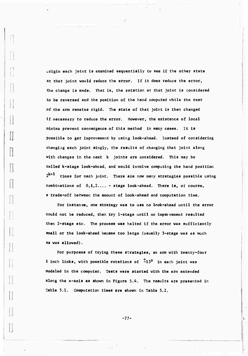
i ■'
0 :
.■
] D D D
D !
i;
!I D
.
D
origin each joint is examined sequentially to see if the other state
at that joint would reduce the error. If it does reduce the error,
the change is made. That is, the rotation at that joint is considered
to be reversed and the position of the hand computed while the rest
of the arm remains rigid. The state of that joint is then changed
if necessary to reduce the error. However, the existence of local
minima prevent convergence of this method in many cases. It is
possible to get improvement by using look-ahead. Instead of considering
changing each joint singly, the results of changing that joint along
with changes in the next k joints are considered. This may be
called k-stage look-ahead, and would involve computing the hand position
k+1 2 times for each joint. There are now many strategies possible using
combinations of 0,1,2.... - stage look-ahead. There is, oi course,
a trade-off between the amount of look-ahead and computation time.
For instance, one strategy was to use no look-ahead until the error
could not be reduced, then try 1-stage until no improvement resulted
then 2-stage etc. The process was halted if the error was sufficiently
small or the look-ahead became too large (usually 3-stage was as much
as was allowed).
For purposes of trying these strategies, an arm with twenty-four
1 inch links, with possible rotations of -15° in each joint was
modeled in the computer. Tests were started with the arm extended
along the x-axis as shown in Figure 5.4. The results are presented in
Table 5.1. Computation times are shown in Table 5.2.
-77-

e <
u
c
■o
a a
so H
s, 3 0
u
>
M
3
M
1^1
M
> O
Z >- M CO
a a
< i
o J
o
u u ?s w
I m
X u X H
W U
gs M
i
a
is < H
U3 Q
O 9 O «N 3 • fe w -H o
• H O M O Z 3
a: o EC
5 Q O UJ M e H U
o B
Q O < z
< H
8
H H v) z
" O CM rj
a UJ
H z
UJ
O
Q U
O H
Q a •< J cfl u3 M u
a M 5 z
i z si i
M O H a:
§^ U H
Ü
O u. z O 1 o K
z o
H U
O a: X cm
s 02
z o H o w M e
o o: x a,
o o J 6 UJ
a w u I
x
0
5
N
§
o
8 Ö
8 0
8 o
(S
o
o o
(^
CD
H 0
8 0
S d
m
0
8 0
io
in
ro
s
8
m
IT)
CO
o
o (3
in
O r
3 in
rO
in
3
«P ro
n
s
If»
-78-
0
0)
Ö
o
J) o
9 9
10
o
o
(N
fO
U)
b
5
<*)
3
OD 10 O
v9
0 0
to
4
ro
±
*
$ ■i
O
in
fO
0
o
1? o
r-
5 o
0
10
o
c
Ifi
8 ab
0
O
n
§
o
o
in 5 o
Q
cr
u)
oo Ö
i
s o
«■^
8 fO
o o
-o tu
3
a» u
c <u E 0) > o 14
|
u x; 4-1
3
o z
E C <
> u B
x: y b IT!
1
C II 3 tr M
a o o
01 c o hi 0
c o
tJ 3
0
01 r-1
i-
u o ES
1
0 «o
u
1
0
o
I
in
Q a
o < 0
U 01 m
J
Of w a.
H
I
I,
Q !"
0
I:
I
1. I L [

i
i I
0
Ö
D n
ü
D II
Figure 5.4. The arbitrarily chosen initial starting configuration for the arm.
It can Se seen that no strategy tried was best in all cases. These
methods had the additional disadvantage that the shape of the arm itself
was not predictable. It was hoped that improvement would result if the
searching was started after the hand was put at a point near the target
by some simple procedure.
In order to place the hind near the target, a curve connecting
the origin and the target was generated, whose arc length was equal to
the length of the arm, and whose curvature did not exceed that which
the arm could assume. Curves made up of segments of four circles having
the above properties were used (details of the derivation of these
circles are presented in Appendix III), and a rought attempt was made
to match the arm to this curve. After the rough curve match, the
previously described searching technique with 1-stage look-ahead was
used. Various curve matching algorithms and different radius circles
were used. Some of the results are shown in Figures 5.5 through 5.9.
Figure 5.5 shows the configuration resulting after four loops with
no look-ahead, then two loops of 1-stage look-ahead. The procedure was
started with the arm aligned along the x-axis as in Figure 5.4.
Figure 5.6 is the result of first matching the arm to a curve composed
-79-
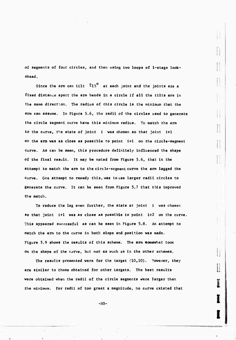
of segments of four circles, and then using two loops of 1-stage look-
ahead.
Since the arm can tilt -lb at each joint and the joints are a
■80-
[I
i
w
I
i:
fixed distance apart the arm bends In a circle if all the tilts are in
the same direct .on. The radius of this circle is the minimum that the
arm can assume. In Figure 5.6, the radii of the circles used to generate
the circle segment curve have this minimum radius. To match the arm
to the curve, tHe state of joint i was chosen so that joint 1+1
on the arm was as close as possible to point 1+1 on the circle-segment
curve. As can be seen, this procedure definitely Influenced the shape
of the final result. It may be noted from Figure 5.6, that in the
attempt to match the arm to the circle-segment curve the arm lagged the
curve. One attempt to remedy this, was to use larger radii circles to
generate the curve. It can be seen from Figure 5.7 that this improved
the match.
To reduce the lag even further, the state at joint 1 was chosen
so that joint 1+1 was as close as possible to point i+2 on the curve.
This appeared successful as can be seen in Figure 5.8. An attempt to
match the arm to the curve in both slope and position was made.
Figure 5.9 shows the results of this scheme. The arm «omewhat tooK
on the shape of the curve, but not as much üS in the other schemes.
The results presented were for the target ^10,10). However, they
are similar to those obtained for other targets. The best results
were obtained when the radii of the circle segments were larger than
the minimum. For radii of too great a magnitude, no curve existed that
i.
i I I

I I
:
i
n
I4i
Figure 5.5, Result of arm after 4 loops of 0 look-ahead and two loops of 1-stage look-ahead. The starting configuration was along the x-axls, as in Fig. 5.4.
-81-

1 ly
«2-
10- Target (10,10)^0
0 ^s^^^^^
8_ 0 0 Points on curve made up or tour V X
circles 0 \^ \ Arm after simple attempt to match li \
curve 0 ^Nt \ *— ^ w "
<o- 1 J. Position of arm after two loops of \^ ) ^^■^ ̂ ■■^T
sequential 1-stage look-ahead search 0 >^
0 \
t- o y
2-
>
O f-
2 4-6 8° o^ffl»—*^i2. ;v
-2- +
[1
■
:.
Q
n
Figure 5.6. Result of trying to match arm to curve made up of segments of four circles, and the improvement after two loops of 1-stage look-ahead. Radii of circles is equal to minimum radius that the arm can assume. The curve matching tech- nique was to choose 0; so that point i+1 on the arm was as close as possible to point i+1 on the curve.
-82-
i.
!.
L I I

i i i i i
::
♦ y
D n
12-
•2-
-4--
Target (10,10)
0 0 Points on curve made jp of four circles
II M Arm after simple attempt to match curve
-f Improvement after two loops of 1-stage look-ahead from above
:
D
Figure 5.7. Similar strategy to that in Fig. 5.6. In this case the radii of the circles Is 1.2 times the minimum radius that the arm could assume.
-83-

Q-
10-
8_
fc-
4-
2-
Target (10,10)
0 Points on curve made up of circle segments
Arm after attempting to match curve
^ Arm after two loops of sequential 1-stage look-ahead
-2_
f]
::
::
r
:
o 1
i
\:
-4-
Figure 5.8. Result of trying to match arm to curve made up of segments of four circles, and Improvement after two loops of 1-stage look-ahead. Radii of circles Is 1.2 times minimum that arm can assume. The curve matching technique used was to sequentially choose 9i so that point 1+1 on the arm was as close as possible to point 1+2 on the curve.
-84-
0
1. i:

■"
ilV
(2-
D
:.
0
:;
::
;:
Target (10,10)-
0 0 Points on curve made up of circle segments
y g Arm after attempt to match curve
1 j Arm after two loops of sequential 1-stage look-ahead
-2-
Figure 5.9. Result of trying to match arm to curve made up of segments of four circles, and improvement after two loops of 1-stage look-ahead. Radii of circles is equal to minimum radius arm can assume. The matching technique was to sequentially choose ^»0 thmtfi^-J^J+^-^sglj^^CJ^U] was a minimum, where (x,.,/,.') is the coordinate of joint i on the arm and (,*i . yj is the coordinate of point i on the curve. This matching criteria puts a weight on the slope as well as the position of the links.
-85-
•
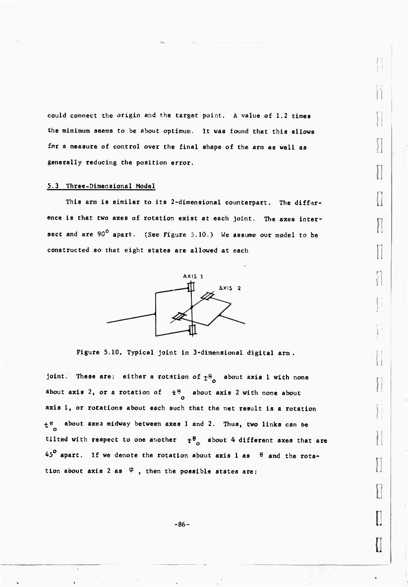
could connect the origin and the target point. A value of 1,2 times
the minimum seems to be about optimum. It was found that this allows
for a measure of control over the final shape of the arm as well as
generally reducing the position error.
5.3 Three-Dimensional Model
This arm is similar to its 2-dimensional counterpart. The differ-
ence is that two axes of rotation exist at each joint. The axes inter-
sect and are 90° apart. (See Figure 5.10.) We assume our model to be
constructed so that eight states are allowed at each
Axis l
AXIS 2
Figure 5.10. Typical joint in 3-dimensional digital arm.
joint. These are: either a rotation of f6 about axis 1 with none - o
about axis 2, or a rotation of -to about axis 2 with none about o
axis 1, or rotations about each such that the net result is a rotati
-^H about axes midway between axes 1 and 2. Thus, two links can be o
tilted with respect to one another t8 about 4 different axes that are
45 apart. If we denote the rotation about axis 1 as Ö and the rota-
tion aoout axis 2 as V , then the possible states are:
on
-86-
w
i:
::
o o ■
;:
I
i
i:
i: i;

■
o Q
D
0 ::
D
::
;;
i
State 9 cp
1 o
0
2 -e o 0
3 0 o
4 0 "Bo
5 +tan (—tan 6o> ain'^-fsinÖ ) 42 0
6 'l 1 +tan (—tan
</2 9o>
-sin-^sme^
7 -tan^ci-tan >/2 ».> -8in_1(-l-8in9 )
8 -tan' (-l-t«n 9o> +8in"1c4-8ln9 )
v/2 o
where the values of 6 and cp in states 5-8 are the actual rotations
about axes 1 and 2, leading to equivalent tilts about axes at 45°
to 1 and 2 (see Appendix III). An n-link arm wouJd then have 8
possible configurations. Again there is a well-defined transformation
to find the position of the hand given the angles (See Appendix III)
but no such transformation exists to find the angles given the hand
position.
The procedure presented in Figure 5.3 is still applicable except
8 states exist at each joint. Then each joint wouH be examined
sequentially and the state at that joint is chosen which minimizes
the Euclidian distance of the hand from the target. With k-stage
look-ahead variations in the joint under consideration plus all
possible ccmbinations of the next k are considered. Then only the
joint under consideration is moved. The position cf the hand must thus
k+1 be computed 8 times for each joint and the time involved in these
computations will limit the amount of possible look-ahead.
-87-

II
0
i: i.
An arm with 24 l-inch links and possible tilt of *15 between each
link, was modeled In the computer. The arm was placed initially in
the configuration of Figure 5.3 and strategies involving combinations
of no look-ahead and 1-stage look-ahead were tried. Results are presented
in Table 5.3. Computation time for one loop of sequential search is
shown in Table 5.4. Details of the algorithms used are in Appendix III.
In general, the results are encouraging. It seems that this
approach works better in three-dimension than in two as the errors
are lower. The reason for the Improved behavior can be attributed to
the additional possible states at each Joint. Computation time is
longer in three dimensions, limiting look-ahead to one stage if real
time problems are to be undertaken by the arm.
', 5.4 Discussion
Many variations of the aforementioned strategies are possible.
For example, one may start sequential searching and making moves at
the hand then work toward the origin. It is also possible to find
the joint at which a change would reduce the error by the largest
amount, make this change, and then continue the process of changing
the joint that makes maximum reduction in error.
A reason for starting at the origin and working toward the hand
is that in general a fixed rotation near the origin will cause the
greatest deflection of the hand. Thus, in many cases making a change
near the origin turns out to be the change that makes the maximum
reduction in error.
Another approach is to take two joints at random and consider
the result of simultaneous changes in each. The two-dimensional
-88-
1
o i.
1.
L

.
0 ;
'■
::
n ;
:;
:
a I:
<
2 o •-< N C
^3 i
m
o
r
—c
-x
M
1-
5
3 M
1
O tN J5 s (0 1 ij oc C o- r-
>- W CO UJ d o Ö r«* 53 « .., < . _ ^ e s c^i 5 O M s % $ H
F 1-
OLLO
TH N 00 o
1 S S
z u 5 O tu M o S N if)
a-o^
8 = OU X
•0 cr «1
1 LOO
AHEA
LOOP
8 N
§ § F-4 gf
1 a: e — (0 05 S H DO OS -H U 0 Ö «J i
iJ Q W ^ ö 0
z 5 P N g § 1 1 i-J C/l
U. J t O O ^ Q
cr § Ä
1 LOO
AHEAD
LOOP 0 M U ^
a. 8 ri
9 § i O u. £ zog N rM (0 ff>
« O <N
Oi —1
o o- 0 g s
Q UJ 0 o 0 o < _; - UJ l-l UJ"
or $ ft B i ^ N r 0 4 H O Q o O UJ -J ra ü
z z a
z w >- « K fi Ä
TAGE
ONTI
OTHI o S
[ - -ru—■ K> f 5 0
M ^
8 en u z i
'75 Oi 6 X 0 a
«T 1 ^ £ r* 2 — —
c u. S z o ffl lO rt * CO
X ■31 u "■ 1 < UJ as <N
* J 8 0 1
CA -3 Q OS c l-l UJ UJ -^ 0 ü "-' o
1EAD
. :D UN
" CHAN^
fl 6 ^ s fj SB ? S9 9
< 3 O i z z
z o O W ? 8 a r- ^ M M ft o r«
5S H H O
C oi X
1
J o o ^ " z s * & p-
z *^ o- ^
N oo 0 CD A bu C Ü •-•
■ o' (O' — OS -w < ^ . ^ < H
X n 2 Oi C«
E
s o
I n
I 8
w c <u
f
UJ Ü
I
UJ
'-O I
s
I § 4J
I
o o
o n
«
u it in
as UJ a,
X >-l
H
I -89-

4 18 volume of 5x10 cubic Inches and 10 reachable points exist, thun
-90-
.
:
curve matching scheme could be extended to threc-dlmenslons to give the
arm a better starting configuration. It might be possible to break the
spatial problems down Into planar problems. Another Idea Is to divide
space up Into several regions, store a configuration that places the
hand In each and then Initially start the hand In the region closest
to the target.
Many strategies are possible, none clearly better than others.
Perhaps further study would show that certain ones work better In certain
areas of space. It then might be possible for the computer to learn
which was best for a particular region.
Different error criteria might be better. Cartesian coordinates,
with the base of the arm aligned along the x-axls were used. This might
mean that error In the x-dlrectlon should be weighted differently than
error In the y- or «-direction. Perhaps the arm can better reduce angu-
lar error than radial error and this should be taken Into account. Again
learning might be applicable In selecting one error criteria for a given
region or for optimizing weights placed on different quantities In an
error function which Is to be minimized.
(i In order that this arm be useful, the points In the reachable space
must be close together. With a 24 link arm, there are 8 (approximately
21 10 ) possible configurations. There will be fewer reachable points than
24 configurations, but reducing 8 by a factor of 10 or 100 or 1000 1.
;:
.
i: still leaves a large number of points. Near the boundary of reachable
space, the points will be further apart, but In the Interior, the
density whould be very high. Assuming that a 24 link arm has a working
L L

I i;
;
:
o
::
D
I
i.
::
13 the average density is 2x10 points per cubic inch, or if the points
were equally spaced, they could be 0.00004 inches apart. This leads
one to believe reachable points should be close enougli to any arbitrary
point in the space. The problem, of course, is to find the configura-
tion that leads to a position near a desired point.
The results indicate that it is possible to find a solution for
this digital manipulator. The solutions obtained are far from optimal
but close enough to be useful. The dimensionality of the problem is
staggering at limes, but it is in fact the large number of solutions
that give hope for any sub-optimal technique.
Further improvement is possible. liv streamlining the subroutines
used for basic computations, computer time could be reduced. The
incorporation of different strategies for different zones would be
useful.
Although the problem of finding a set of angles to place the hand
at a given target appears soluble, the arm itself has serious limitations.
The primary drawback is the inability to control its motion. Since
there are discrete states at each joint, a wild motion is likely as
each change is made. That is, the position is undefined when motion
occurs. In addition, positions close in spac may be very different in
arm configuration. In conclusion, the arm is interesting but in its
present state has no immediate usefulness.
•91-
!'

B~
I
BLANK PAGE

11
0 ;
:;
n
;
u i:
D :.
D D i!
CHAPTER VI
TRAJECTORY GENERATION
6.1 Problem Statement
In remote manipulation a typical problem is to move from an initial
configuration to some new position and then to grasp an object. In
order to carry out this task, the position problem must be solved. This
results in a set of values specifying how much to rotate each joint in
order to move the manipulator from its current or initial configuration
>o the desired final state. However, in such a case no explicit infor-
mation exists describing the intermediate states between the initial and
final position. It should be noted that the initial and the final
configurations may be physically far apart, and the s, ace through which
the manipulator must move to attain the final state will in general
contain obstacles. It is therefore necessary to find a "path" along
which the manipulator can move and not collide with any of the obstacles.
This problem will be referred to as trajectory generation. We attempt
to solve this by defining sets of intermediate values for the joint
anglet; which lead the manipulator to the final state in a manner which
avoids collisions.
A person performing manipulative tasks avoids obstacles very simply.
His eyes observe a possible conflict and he knows intuitively to raise
his ( bow or change his direction slightly. He sees "the world" in
which he is working. He knows immediately which objects he is likely to
encounter and which he will not come near. For a computer controlled
-92-

manipulator the problem is not so simple. The problems of "world"
modeling, conflict detection, and collision avoidance must all be fa(..>d
in order to generate a trajectory between initial and final manipulator
configurations.
As a first step in dealing with this very difficult problem, a set
of routines have been developed that provide a mathematical description
of the world. Other routines simulate proposed trajectories through
the space and sequentially examine points along the trajectory for
obstacle conflict. If conflict is detected these routines suitably
modify the trajectory. Several basic strategies to get from the initial
to the final position are programmed so that if one fails, another can
be explored. A block diagram of this system is shown in Figure 6.1.
In the development of these routines, an attempt has been made to
be as general as possible in order that the programs be applicable to
any manipulator, performing a wide variety of tasks. In the next
sections, we present a description of these routines.
6.2 World Model, Obstacle Description, and Conflict Detection
For this system a simple model of the "world" is used. The basic
elements of the world are assumed to be: planes, spheres and cylinders.
It is assumed that all objects of interest can be modeled with these
elements.
The boundaries of the workspace, usually formed by table tops or
walls, are modeltd as infinite planes. These planes are represented by
a unit vector, b, and by scalar t. Vector b is normal to the plane and
points inward toward the workspace. Scalar t, the distance of the plane
from the origin, is measured in the b - direction.
-93-
r
D
I
I;
!
!,
!.
i;
L L

:;
i :
D i:
D D I
D 0 r
i
-94-
' ^
in w)
^ < Ui
2 J UI 4 u 2 i Ü
1) —•
^2 0
ao c
U
a 75
S
D
u 0 i-l o 0)
M
I
ig
y 0 .-i ca
0)
.

Simple, somewhat regular objects which are not planar or cylindrical
in shape are modeled as the smallest sphere that circumscribes the
object. A typical object modeled in this manner might be a cube, a
pencil sharpener or a coffee cup. The assumption is made that all such
objects are supported by an infinite plane. Thus we represent a sphere
by a, a vector describing the location of its center, b, a unit vector
from the direction of support, and t, the radius of the sphere.
Cylinders are used to model objects containing a predominant axis
such as a tower. In addition, cylinders are building blocks for more
complex objects. For example, a manipulator is modeled as a group of
cylinders each of which corresponds to one of the manipulator's
structural members. The assumption is made that all cylinders are
supported from an infinite plane or from another cylinder. We then
represent a cylinder by a line segment corresponding to its axis and by
the maximum distance of points in the object from this line, d. We have
then:
b: a unit vector parallel to the axis pointing away
from the direction of support
a: a vector describing the position of the base of
the axis
t: the length of the axis
d: the radius of the cylinder
With this representation it is convenient to consider the cylinders to
have a hemisphere capped on each end thereby assuring that all points on
the surface have the same minimum distance, d from the line segment
representing the axis.
-95-
r
■
ö
1
i I:
1. L

i
fl Each obstacle, then, has a list of properties which include its
type (plane, sphere, or cylinder), the composite object to which it
belongs, and the aforementioned parameters which are required for its
quantitative representation. The interpretation of a, b, t and d is
varied according to the type of the object. Such models of all objects
considered to be obstacles to the manipulator are stored in the computer.
The process of conflict detection consists of determining if the
manipulator and the objects in its workspace will be brought to the same
place at the same time. This is accomplished by computing the distance
between the elements of the manipulator and the elements of the work-
space at various positions along the proposed trajectory. A conflict
is then predicted if this distance becomes too small.
It is undesirable to compute the distance between the manipulator
and all of the objects in the workspace. To consider all the objects at
each position along the trajectory would be time consuming. In addition,
much of this computation would be wasted as for an arbitrary position,
the manipulator would be so far from a large number of objects that a
collision with these would be very unlikely. We would thus like to
consider only objects near the manipulator. For this reason we divide
the reachable space of the manipulator into small regions. In all the
i-i work to date, sixty-four subdivisions have been used. The workspace is
considered to be a rectangular parallelapiped with edges parallel to
the axes of a fixed Cartesian coordinate system. The small regions are
defined as the volumes between three sets of equally spaced planes parallel
to each of three mutually orthogonal faces of the workspace. Then a list
of objects completely or partially inside each region is associated with
-96-
n
:.
D D

that region. For conflict detection, only the objects occupying the same
region or regions as the manipulator are considered.
As a result ot dividing the space into regions, we have the problem
of finding in which region(s) various obstacles are located. In addition
we will have to identify the region(s) the manipulator occupies at various
positions along its trajectory. We wish to keep this analysis simple in
order that the time saved in not having to deal with all obstacles in
the workspace is not lost in trying to locate the manipulator in various
regions. Since the faces of our subdivisions are made perpendicular to
the coordinate axes, we can easily eliminate many regions by comparing
the minimum and maximum coordinates (x, y, z) of an obstacle, with the
coordinate boundaries of the regions. To find in which of the remaining
regions an obstacle lies we compute the distance from the center of each
of the regions to the obstacle (a fairly simple process in view of the
simple world model). We thencompare this distance with the radius of
a sphere totally enclosing the region to determine if the object is in
the sphere. If the object is in the sphere, we assume it to be in the
region. This procedure may cause an object to be considered inside a
region when in reality it is outside. However, this process is con-
siderably simpler than trying to find whether an object cuts any part
of the actual region.
Routines were developed which divide space into regions and
appropriately enter or remove objects from lists associated with the
regions. These routines also store the properties of each obstacle.
The conflict detection routine starts with the first link of the
manipulator and finds which regions this link is in. It then finds the
-97-
:
w ■
o T
1
1.1
;
i:
i.
L

w
:
::
:
n ü
ü D U D
distances between all the objects in these regions and the link. A
collision is predicted if the distance between any object and the link
is small enough so that, with the link continuing along its present
course, a conflict would occur. If a collision is predicted, a flag is
set and the routine specifics the obstacle and the link closest to the
obstacle. It no collision is detected the procedure is carried out for
the remaining links in the manipulator. A block diagram of this program
is presented in Figure 6.2.
The method for determining distance between a manipulator link and
an object depends upon the type of object. For spherical objects, the
distance between the sphere center and the cylinder-axis of the link is
computed. The actual distance is then found by decreasing this by the
sum of the radii of the sphere and the cylinder (representing the link).
For planes, the distance between the plane and the cylinder-axis of the
link is computed. This distance is decreased by the radius of the
cylinder to form the actual distance. For objects modeled as cylinders,
we find the distance between the object axis and link axis, and decrease
this by the combined radii of the cylinders. Details of these calculations
are found in Appendix IV.
6.3 Trajectory Generation and Obstacle Avoidance
We have the problem of finding a series of closely spaced inter-
mediate positions connecting initial and final states. These represent
a trajectory that the manipulator can follow while avoiding all obstacles
in the workspace. The approach used is to start by choosing a plausible
trajectory, simulate the motion along the trajectory and then if conflict
-98-

START
_L LINK ■ l
FIND PHYSICAL. DESCRIPTION OP LltSK.
1 FIND WiHICH REGIONS LIMK IS IN
1 CET I_IS1 OF REGIONS AND
OBSTACLES IN THESE NUMBER OF OSSTACuES
LINK»LINK-»- I
OBST =
ZZE OBST= OBST + I
FIND DISTANCE BETWEEN LINK AMD CVUNDEiR
f'iNC DISTANCE BETWJEetM LIN^
f
FIND DlSTMMCE BETWEEN l-INlC AND SPWE«E
vee
FIND LINK THAT
HAS MINIMUM
DISTANCE TO
OBST
SET FLAG 1 —'
VE5
EXIT
-
11
i.
\
ICXIT
Figure 6.2. Block diagram for conflict detection routine,
•99- 1. [

:
;
I
!;
occurs, to modify the trajectory. This modification is made on the basis
of local geometric conditions in the area of conflict. (A program,
called AVOID, accomplishing this will be discussed in more detail later
in this section.)
Often if more than one obstacle is present, a move that appears
good to avoid one obstacle is bad to avoid another. This may lead the
manipulator to oscillate between objects. It is also possible for somf
joints to be at their physical limits so that the avoidance routine does
not find a good move. Finally, the avoidance routine itself may come up
with a non-productive move. It is therefore necessary to continually
ascertain whether or not progress is being made toward the goal. If no
progress is being made, it is then necessary to decide whether a slight
change in strategy is sufficient or whether a whole new strategy is in
order.
A program based on the above approach called TRLTRJ, has been
written. The inputs to the program are two sets of joint angles, one
set specifying the initial position and the other specifying the final
position. In addition the desired increment between intermediate
positions is specified. The output from the program is an array of
angles specifying the intermediate positions.
Four basic strategies are built into the program. The first, and
least complex, just increments each angle towards the final goal. The
second strategy computes two intermediate positions to move the '.ianipu-
lator up and then over a concentration of obstacles. The third and
fourth strategies both try to fold the manipulator to shorten it and then
move it in front of any obstacles. These last two differ in that one
-100-
Ü

-
fl shortens the manipulator by moving Joints in one direction toward the
physical stops while the other folds the manipulator by moving the joints
toward the stops in the other direction (in the program, we call these
directions positive and negative, respectively).
The program starts by trying the first strategy. If any obstacle
is encountered, this strategy is abandoned for the time being and the
second strategy started. If while pursuing this second basic strategy,
a conflict is predicted, an attempt is made to modify the trajectory
using the program AVOID. If "his strategy fails after using AVOID the program
continues and tries the third and finally, if necessary, the "our strategy
in a similar manner. If the fourth strategy fails, the program returns to
the first strategy and tries it using AVOID. If it does not produce a
trajectory, it is assumed that all obstacle avoidance strategies have
failed and the program halts.
If any of the following occur, the program considers that no progress
is being made and hence a strategy has failed:
1. The avoidance routine (AVOID) is not able to generate a
move due to joints being at their physical stops.
2. A collision is predicted with the manipulator at the same
point on the trajectory where a conflict had previously
been predicted with that same obstacle (hence it is
assumed the program is in a loop).
3. A conflict is predicted with a plane for the second
time, while trying to avoid the same obstacle.
(Assumedly we cannot get around the obstacle.)
•101-
11
t
i.
!
i.

:
i
;
I]
Q
U D
The manipulator oscillates between two obstacles, and no
net progress toward a goal is being made.
More than 200 Intermediate sets of angles have been
selected without the manipulator reaching a goal.
More than 350 intermediate sets of angles have been
explored.
The following conditions cause a slight change in strategy but do
not cause the strategy to be abandoned.
1. A plane of infinite extent is encountered while trying
11 to avoid an obstacle. At this point we assume that
the manipulator it moving in the wrong direction to go
around this obstacle. The strategy is to go back to the
first point we encountered this obstacle and try to go
around it by going in the opposite direction. (This
notion of direction will become more clear with the
description of AVOID.)
2. An oscillation of the manipulator between two obstacles
is detected. The action that the program takes is to
go back to the point where the second of the obstacles
was encountered and try to go around it in the opposite
direction. If this happens twice at the same position
on the trajectory, it is assumed that no progress is
being made and the strategy has failed.
A block diagram of TRLTRJ is presented in Figure 6.3.
The subroutine AVOID is used to generate small perterbations in a
trajectory when conflict is predicted. The program attempts to define
-102-

1 START
INITIALIZE PARAMETERS
I COMPUTE POSITION OF A.Rtv> KT PlNAL POSITION
SKT FLAG EXIT
TÄR&6T PsN&LE'
PRESENT ANCLES F^NAL ANGLES
INITIAL ANGLES
COMPUTE NUMfeBROP INCREMENTS BETWEEN PRESENT ANDT^RUET, ft^Ag
TARGET«-FIRST INTSRMtWMä t TA«aiT T.
COMPOTE TVsiO »NTtR- MEDtAJE GOALS ONE NCA« INITIAL fosrriCN THECTTHER NEAR PIN AL POSITION ©an«
Figure 6.3. Block diagram of fklTRJ
-103-
i:
1: f. C
r
I:
!
I.
1, I E I

fl
a "gool" direction and a "bad" direction. It then tries to move the
link for which a collision has been predicted as much as possible in the
good direction while not moving in the bad direction. This is accomplished 1
by defining small changes in the Joint angles of all the links between the
base and the "colliding" link. Ideally these angle changes are chosen so
that the link will have a large velocity component in the good direction
and zero component in the bad direction. If the link does not have enough
freedom (i.e., there are too few joints preceding the link or the joints
are at their physical stops) to make a move in this manner, an attempt
is nude to move in the negative bad-direction. If this too is not
possible then no move is made and a flag is set indicating that the
strategy has failed.
The underlying idea used in choosing a good direction is that all
obstacles are supported by either an infinite plane or another obstacle.
Then if an obstacle lies between the manipulator and the target, one
could eventually get around the obstacle by moving away from the direction
of support. In addition an attempt is made to move in the general
direction of the target. This target will normally be the final position
but may be an intermediate goal generated in a strategy of TRLTRJ. If
the predicted^conflict has occurred in the process of avoiding a different
obstacle, the target becomes the position generated by AVOID when the
manipulator encountered the first obstacle. The good direction is chosen
taking into account the type of obsta > and the relation between link,
obstacle and targe«- as follows;
If the obstacle is a plane or a sphere, the good direction is
specified by a vector from the point of conflict on the link to the same
n
D n
D 0
D I! 0 0
•104-

point on the link with the manipulator at the target position. (The
assumption here is that the sphere is relatively small and lies on the
plane of support.)
If the obstacle is a cylinder, then the process is a bit more
complicated. Recall that a cylinder may be part of a more complex
obstacle (for example the towers in Figure 6.4). If no other part of
the possibly complex obstacle, of which the cylindrical obstacle is a
member has been recently encountered, then the good direction is:
1. The direction of the axis of cylinder, if the
obstacle appears* to be between th^ manipulator and
the target.
2. The vector sum of unit vectors in the axis direction
and the direction the link must move to get to the
target, if the "ink is above the cylinder.
3. The direction the link must move to get to the
target, if obstacle is not between the manipulator
and the target.
When the cylindrical obstacle is part of a more complex obstacle
and when an element of this complex obstacle has been previously en-
countered, then the good direction is similar to the above with the
following exception: the positive axis direction is replaced by the
negative axis direction whenever the point of conflict on the obstacle
is nearer the far end of the obstacle (i.e., away from the point of
*We say "appears" because a cylindrical object may not itself be between the manipulator and the goal, but the complex obstacle which it belongs to, may indeed be between the manipulator and the goal.
•105-
I:
I
0 i;
i
i
i.
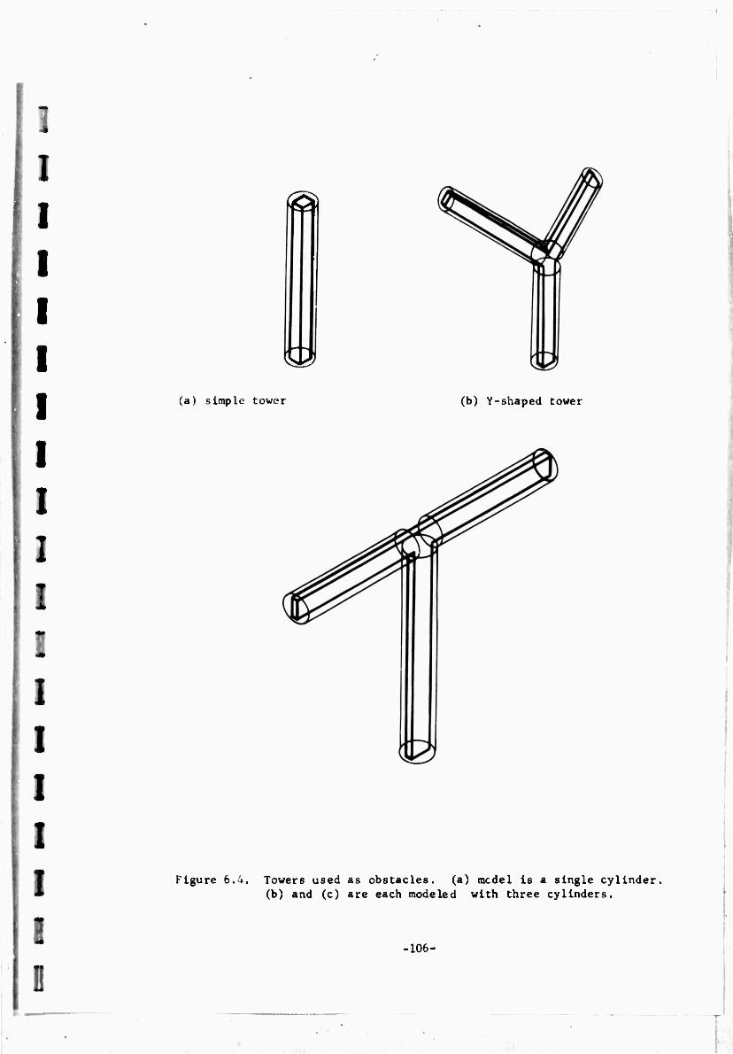
i (a) simple tower (b) Y-shaped tower
!
ii
Figure 6.4, Towers used as obstacles. (a) mcdel is a single cylinder (b) and (c) are each modeled with three cylinders.
-106-

support). In this way we are able to follow the contour of a complex
obstacle.
Once a good direction has been established for an obstacle it
remains the same until:
1. The manipulator is clear of the obstacles, or
2. An oscillation has been detected;by TRLTRJ, in
which case wherever the positive axis direction
was to be used, it is to be replaced by the negative
axis direction and vice-versa.
The bad direction is always specified by a vector from the link to
the obstacle, along the line defining the minimum distance between them.
A block diagram of AVOID is presented in Figure 6.5.
6.4 A Test of the Program
The trajectory generating routines were tested by incorporating
them into the block stacking program developed at the Stanford
Artificial Intelligence Project L25J. The block stacking program
represents current research work in hand-eye systems. An electric
motor driven manipulator of type 6R, So a^ s^ a,- (see Figure 6.6) and
a vidicon T.V., interfaced with the PDP-6 computer form the basic system.
Programs written by Singer and Pingle [25J enable the manipulator to pick
up blocks from a table and build block towers. The blocks are originally
placed at random on the table but within view of the vidicon. A block
is then located on the table by appropriate analysis of the T.V. picture.
Next, the manipulator moves to grasp the block and then places it to
build a tower. A new block is found and the process continues.
-107-
[j
■
1.
!
1
i,
L 1.

:
I :
::
i
0 D l
Ö
D
STAfRT
INITIALIZE PARAMETER G.OOD JOINTS.O.BAD iOIK4T5=0,
I ^1
INPUTS TARGET POSITION PRESENT POSITION
PIND A COOO DIRECTION TO MOVE NOTE: (ME ARE MS3* Wv^ .NOTi Twe
JO«"TS oseo TO
0-*- DISTANCE POINT OF COUUISION TRAVELS VN 3 TtMtSTdPS
0«- 0-Cl*TfcNCE. MOVED IN GOOD DiBECTlON
MOVS. IM
^ETC IIMTUE GOOD
DIRECTION iVEI-V.
CHOOSE JOINT THAT MOVES POINT OF COLLISION POSSIßLE USE'aOOO
ON ARM AS MUCH AS IN GOOD DIRECTION, DO NOT JOINTS OR '»AD" JO(NTS
[THIS JOINT IS A COOP JOINT
COMPUTE ANGLE CHANGE INTWiS JOINT TO MOV« POINT OF COLLISION DISTANCE D IN GOOD OIR&CTIQN
MOVE JOINT AS FAR AS POSSIBLE COMPUTE WOW FAR IS MOVED IN GOOD DIRECTION
REDUCE CHANC1 SO STOPS NOT EXCEEDED
j SET FUAG.
Figure 6,5. Block diagram of AVOID.
-108-

Figure 6.6. Electric Arm at Stanford Artificial Intelligence Project. A prothef tic arm originally built at Rancho Los Amigos Hospital, this arm has been modified for use In hand-eye research.
-109-
r
l:
0
n !
W
1
i
1: i
L
I.

i
G
Q :
0
ii
0 I
i
0 11
I!
II
The trajectory generating routine is used to find trajectories when-
ever the arm is moved except in the last stages of actually picking up
or setting down a block. At these times, the manipulator control is
transferred to a special routine whose function is to lower or raise the
hand along a specified path with a specified orientation.
Objects considered to be obstacles are the table top, the support
structure for the arm, and any block towers that have been built. In
addition, to make life difficult for the program, several other obstacles
(see Figure 6.4) were added. Since the range of vision of the T.V.
camera is small, and its recognition powers to date is limited to cubes,
a sub-program was written so that the external obstacles could be added
to the data structure by commands from the teletype.
After allowing the program to run, with the different obstacles in
varying locations, the trajectory generation program was seen to perform
fairly well (see Figure 6.7). Where possible, it was generally able to
go over or in front of the obstacles. However, the procedure occasionally
failed when the manipulator wrs started in a configuration in which joints
were near their physical stops. In these cases a successful maneuver
might have been to move thosf joints well away from the stops and trv
again (a procedure not built into the program). In addition, if the
objects were so placed that the arm could only get through by going
between two objects, failure generally occurred.
Whenever more than one or two strategies were tried, the computation
might run upwards of 20 seconds. However, most manipulative scenes are
fairly static, so that once a trajectory had been found through a given
set of obstacles, it could be used repeatedly. This process would save
-110-

fl
i.
Figure 6.7. Example of trajectory enabling manipulator to go over obstacles.
I:
I:
n i
G
!
n
-in-
i:
i
I:

n
o D 0 :!
D n 1J
o D D ;:
G D
having to re-analyze the trajectory for every move, thus conserving
computer time. In addition we could move backward on the same trajectory
to get back through the space again.
With this program we have attacked the problem of moving a multi-
link manipulator through a space composed of three-dimensional objects.
Had we been concerned with having Just the hand avoid obstacles on a
plane, the problem would have been much less complex, as the hand could
be made to follow an arbitrary curve. Such is not the case, when
considering a conflict with all links of a manipulator. We cannot inde-
pendently specify the position of each link of a six degree-of-freedom
manipulator. There are just not enough freedoms. However, the programs
developed above do enable us to deal with the problem of conflict for a
general multi-link manipulator. These programs perform the basic
function of allowing a manipulator to perform tasks in the presence of
obstacles.
•112-

BLANK PAGE

:
0 11
;:
D D
*The iterative technique may however be used to good advantage when the distance between positions is very small. Then the iterations converge quickly, and there is only one solution being sought.
CHAPTER VII
CRITERIA IN THE DESIGN OF A MANIPULATOR FOR COMPUTER CONTROL
7.1 Kinematic Criteria
As mentioned earlier, a manipulator needs to have six degrees-of-
freedom to grasp a rigid body with a specified orientation at a specified
position in space. In addition, the kinematic solution must be easily
programmed and solved. This indicates the desirability of a closed-form
solution rather than iterative techniques. The closed-form solutions
are faster and find all configurations leading to the desired terminal
position and orientation while iterative techniques find only one.*
In fact, the iterative schemes may not find a solution even though
several may exist. The question of the existence of a solution is
importdnt, as this existence indicates whether a given position and
orientation is physically attainable. It is desirable to have solutions
exist throughout th^ workspace or at least know where they do not exist.
Thus a factor in the design of a manipulator is the zones in which the
terminal device can be placed in an arbitrary manner.
The problem of zones is closely allied to that of solutions. The
existence of a solution for a given position and orientation automatically
guarantees that that point is within the zone of reachable points. One
method of investigating zones would be to solve the position problem for
113- ,

many points and many manipulator configurations. This however Is very
lengthy and not at all general. Alternatively, we attempt to give a few
general remarks about zones.
When on the boundary of the zone of reachable space, the hand
cannot be moved In an arbitrary direction or rotated about an arbitrary
axis. Another way of saying this Is that the hand cannot move along an
arbitrary screw. Mathematically this happens' whenever the determinant
formed from the left-hand sides of equations (4.13) and (4.14) vanishes.
The existence of a solution would enable us to express the W and r ,
appearing In (4.13) and (4.14), In terms of the hand position and
orientation. Then forming the determinant we would have a polynomial in
terms of the hand position and orientation whose vanishing would correspond
to the boundary of reachable space. We .rould then have a surface in
six-space which bounds reachable space.
As this representation is highly non-linear, as well as dependent
upon the existence of a solution, it is often more fruitful to examine
the problem from a geometrical viewpoint. For example, consider the
611,8381; manipulator with all adjacent pairs of axes perpendicular, as
is shown in Figure 7.1. We note that the wrist point, W , defined by
the vector P , can lie anywhere within a sphere of radius r about the
shoulder point, 0 , where.
(83-«5)2^ r2^ (^^j)2 (7.1)
Furthermore, if the wrist position is fixed, then the direction the
hand points, defined by a^ in Figure 7.1, is arbitrary. Through
appropriate rotations in joints 3 and 6, a6 can be made to point in
any direction. However, the total orientation of the hand cannot be
-114-
li
-
0 r _
"
■"'
■"
■
___
_ •
_
■
1
D
D
11 1 I I !
I I fl D Q
I I: !:
D
0 0
arbitrarily specified for a fixed wrist point as tha direction defined
by aig In Figure 7.1 is limited in range. We note that ^ must
always be perpendicular to mg . Hence, ^ may lie anywhere in a
plane perpendicular to ^ . Now the specification of the wrist
point does not fix the elbow point, A, and in fact the triangle QAW may
be rotated about P . We observe, then, that (V, must lie on a cone
whose axis is P , with apex at W and whose cone angle is fixed by
triangle QAW. Then * will lie in planes through W , perpendicular 6
to the elements of this cone. This defines a second cone, inside which
^, can never point. These cones are shown in Figure 7.2. Referring to
Figure 7.2, the elements of cone 1 form the locus of w while *» will —3 o
always lie outside cone 2.
If it is desirable for the hand to have a full range of orientation
freedom, then a manipulator whose, last three Joints are revolute and
whose axes intersect is appropriate. Consider such a configuration,
shown in Figure 3.8. Here the last three axes intersect and provide
maximum orientation freedom for the hand. In addition this configuration
has a wide range of positions that the wrist point, defined by P-j ,
can assume. Referring to Figure 3.8 we note that the wrist point can be
placed anywhere Inside a circle normal to axis 2, about ?■, , whose radius
r obeys the constraint:
(a2-s4)2 ^ r2< (a2+s4)
2 (7.2)
Rotation of the first Joint then rotates this circular anulus to generate
a torus which is the locus of points the wrist can reach.
It is possible to examine many manipulator configurations in this
manner. Table 7.1 presents the results of such examination of 6R manipu-
lators with two and three non-zero link parameters. Whether or not a
solution exists is also included in Table 7.1.
-115-
D

"— ■»
Figure 7.1. A 6R,8-S manipulator
CONE 2
Figure 7.2. Cones showing possible loci for bJ» and <i?c
-116-
n D II 0 li
II
n I! 1 D
I
li
l!
i:
L 0 II I

fj
11
• - . ■ . . • -
TABLE 7.1
Solubility and Orientation Restrictions in 6JV Manipulatoru
o D D i;
fi
[i
o 0 I! D
MANIPULATOR REMARK MANIPULATOR REMARK MANIPULATOR REMARK
1 a182 D 16. 8283 D 31. 84a4 D
2. a^j D 17. a2a3 S G 32. S4S5 D
3. a s 1 3
D 18. 3284 S G 33. s4a5 D
4. .j.3 S G 19. a2a4 N R 34. a4s5 D
5- al84 S G 20. 8285 S R 35. a4a5 D
6. a^ S G 21. 8285 S R 36. s5a5 D
7. a1s5 D 22. 8383 D 37. 8^8282 D
8. a^ D 23. S3S4 S G 38. ais2s3 D
9. 8282 D 24. 8384 S G 39. a^a-j S G
10. 8280 P 25. 8385 S R 40. a1S284 S G
LI. B2&2 S G 26. 8383 S R 41. a182a4 S G
12. 8284 S G 27. 8384 D 42. 8^285 D
13. 82»^ S G 28. 8384 S G 43. V2«3 D
14. 828c D 29. a385 S R 44. aia2s3 D
15. 82a5 D 30. a3a5 S R 45. a.a2a.i S G
-117-

Table 7.1 (continued)
MANIPULATOR REMARK MANIPULATOR REMARK MANIPULATOR REMARK
Ub. a1a2«4 S G 63. a,a.ar 14 5 S R 80. S28484 S G
U7. a1a2a4 N R 64. a^s5ac D 81. 3284s5 S G
U8. 0^2^^ S R 65. 828283 S G 82. 8284r5 S R
U9. a-^a^a^ S G 66. s^a^a-i S G 83. 82a485 S G
50. a183a3 S G 67. 828284 S G 84. 82a4a5 S R
51. a183s4 S G 68. 828284 N R 85. 8^8,. D
52. a183a4 N G 69. s2a2s5 S R 86. 828383 S G
53. a]S3S5 S R 70. 828283 S R 87. 82S384 S G
54. a183«5 S R 71. 8^383 S G 88. 328-58/ N G
55. a1a384 S G 72. 828384 S G 89. 828383 S R
56. a1a3a4 N R 73. 82S384 N R 90. 828383 S R
57. a^aßSr, N R 74. 8^38- S R 91. a28384 S G
58. a.a^a. N R 75. 8^385 S R 92. a2a3a4 N R
59. a,s.a. 14 4
S G 76. 82a384 S G 93. a2a3s5 N R
bO. a.8.sc 14 5 S R 77. 8283a4 N R 94. 828383 N R
u. .lV3 S R 78. 82a3s5 N R 95. 828484 N R
it, «l-485 S R 79. 828385 N R 96. 828483 N R
•llf-
fl
D fl
i
i: 0 II

0 il
I I 1 I fl
fl Ü
D D D II II D I (i D
Table 7.1 (continued)
MANIPULATOR REMARK MANIPUIATOR REMARK MANIPULATOR REMARK
97. a sa 2 4 5
N R 1
, /5. 838484 S G 113. 838433 S R
98. a2a485 N R 106, S38485 S R 114. 838^5 S R
99. a2a4a5 N R 107. 83.S485 S R 115. 338483 S R
100. ajSjaj S R 108. 838485 S k 116. 838383 S R
101. 83a3S4 S G 109. 838485 S R 117. 8^8485 D
102. 83838^ S G 110. 838383 S R 118. 8^483 D
103. 838383 S R 111. 838483 S G 119. 848583 D
104. 838383 S R 112. 83S4S3 S R 120. 848585 D
Key to Remarks: D - degenerate S - Soluble N - Insoluble
R - Restricted orientation for reachable wrist positions
G - No orientation restriction for reachable wrist positions
-119-

7.2 Additional Considerations
Aside from kinematic considerations, there are many less objective
criteria In choosing a manipulator for use with a computer system. For
the iahe of completeness we mention some of these additional considerations,
and give a few remarks about several of the more Important ones.
1. Ease of Interface with a Digital Computer.
The actuators of a manipulator must be such that their
control may be easily assumed by a digital computer.
In addition position feedback must be available.
This will generally be from potentiometer or shaft
encoders.
2. Power Source.
Manipulators are in general electrically, hydraulically, or
pneumatically powered. Electricity is universally available
and inexpensive. Hydraulic power provides the means for
converting a large amount ot energy to motion with a
minimum of weight, thus an advantage where speed is
required. Pneumatically powered manipulators, working
off of air, are cleaner than hydraulic systems. However,
for safety reasons, they must operate at a much lower
pressure and therefore will have poorer dynamic response.
3. Structural Rigidity.
The structural members must have a minimum deformation
under load so that the position of the hand may be
accurately computed from the rotations in the Joints.
D ii D 0 0 0 n D !l
D
0 1: D D i:
•120- I 0

D il
11 In aaHition the Joints must contain a minimum of play
for the same reason.
4. Range of Freedom
It is desirable that each Joint of a manipulator possess
a large range. Even though a position might be reachable
from a kinematic point of view, the physical limits on
actuators will greatly reduce the range of these. In
fact, many of the problems encountered while using the
obstacle avoidance programs were due to the very
restricted range of motion on the electric arm
(Figure 6.6).
5. The Outline of the Manipulator.
W« would like the manipulator to have a slim outline
so that it could work in tight places. In addition
a smooth profile might be desirable so that it would
be easily recognizable in a T.V. image.
6. Other Factors.
D il 0 11 I! D I: D II 0 0 I! II 0 !'
Additional factors to be considered are: precision,
speed, cost controllability (i.e., the ability to
follow a prescribed path), and safety.
When choosing a manipulator we cannot hope to maximize all of these
considerations. Many of these are Influenced by the type of task per-
formed by the manipulator. For example, if a goal for the hand-eye system
Is to assemble a machine containing small electronic components, the
manipulator must be capable of very delicate movement and position
accuracy. For tasks involving throwing or catching objects, the arm
-121-

n must be able to move rapidly, and be accurately controlled. Thus some
applications require obvious tradeoffs (e.g., precision and speed),
and in others certain considerations predominate.
From experience with the two manipulators uaed at the Stanford
Artificial Intelligence Project we may make some comment on specific
arms. The project presently aas two arms. One is a modified electric
prosthetic arm (Figure 6.6). The other is hydraulically powered
(Figure 7.3).
The d.c. electric motor driven arm has proven acceptable for
stacking blocks. After some experimentation, a rate modulated pulse
dc system seems to be an excellent way to control the arm. With position
feedback via potentiometers, and an external pover supply, it is
satisfactorily interfaced with the computer. owever, it is somewhat
lacking in the range of freedom and structural integrity - problems that
could be overcome with a second generation arm of this type. It is not
particularly fast nor particularly precise. The precision problem stems
partly from the poor structure, and partly from the control problem
caused by the inherent inertia in the motors. It is expected that with
refinement of the control scheme, the precision and controllability could
be considerably improved.
Although experience with the hydraulic arm Is limited at this time,
it shows promise of great speed. It also appears structurally sound,
and has a wide range of freedom in its Joints. It is somewhat massive
due to its high speed and torque capabilities. At this time, the control
problem using two-stage servo-valves appears soluble. The physical danger
to personnel and equipment is obvious and this arm is housed in a room
-122-
I:
D fi
r
D
D
I
D i:
D
Ii 0
0
II

D 10
Q
H 0 n
H
D
I! 0 0 D D li
!i Figure 7.3. Hydraulic Am at Stanford Artificial Intelligence Project.
•123-

'
Isolated from the computer. This makes the interface with the computer
T.V. system difficult, though soluble. la addition the forces involved
require that the arm be firmly anchored to the floor.
At present these manipulators are used for fairly simple tasks.
As the hand-eye program becomes more advanced the tasks will become
more involved. At some future time, then, one might expect to be able
to say more about choosing a manipulator for computer control in a more
complex environment.
•124-
r, i!
I
D 11 0
e
o i. i: |-
I:
!.
y IT L

——
I.
I
0 0
n
n D I fl
D D 0 c 0
Ö
II
Q
CHAPTER VIII
CONCLUSIONS AND SUGGESTIONS FOR FUTURE WORK
In this dissertation, the kinematic problems associated with
manipulators have been explored. It Is hoped that the classification
scheme and catalog of manipulators, presented In Chapter II, will lead
to manipulators being compared on a scientific basis. Manipulators whose
exteriors seem much different, are often klnematlcally equivalent. Thus
solutions for one manipulator are applicable to another.
It Is seen that the problem of positioning a manipulator Is directly
related to the displacement analysis of mechanisms. The solutions
presented for cases with three revolute axes Intersecting at a point
seem to be previously unknown. These results therefore represent a
contribution to spatial linkage analysis.
It is felt that these solutions, along with the extension to the
special cases with only pairs of axes intersecting, give insight into
the kinematic analysis problem for the most general six degree-of-
freedom manipulator. That is, for the special case of three intersecting
pairs of axes, four different configurations were found leading to the
same hand position and orientation. For two pairs of intersecting axes,
eight configurations were found, and for only one pair of axes inter-
secting, sixteen configurations were shown to be possible. In all of
these special cases, adjacent axes were orthogonal, and the adjacent
common normals intersected one another. Since no axes nor adjacent
common normals intersect in the most general problem, it is almost
-125-

•126-
I
I
1
D r D 0 D 1:
certain that the general problem has even more possible configurations
leading to the same hand position and orientation.
The possibility of a very large number of configurations indicates
that, even if a solution to the general problem could be expressed as a
single polynomial in one unknown, tuis polynomial would be of such a high
degree that it would be impossible to find all the roots. We conclude,
then, that the complete solution to the most general problem is not at
this time technically feasible: perhaps, someone, someday will solve the
problem. Kinematicians have been trying for over 50 years.
The iterative technique, based on velocity, was found to be superior
to the Newton-Raphson method both in the amount of time taken per iteration,
and in the range of distance between positions where convergence occurred.
The iterative technique may be used to good advantage when tbe distance
between positions is small. Thus an approximate model having a closed
form solution could be used to find starting points from which the
numerical procedure could be used to find actual solutions.
The problem of placing the end of a digital manipulator at a target
appears soluble. The results have shown that the hand can be placed
close to an arbitrary point. Different strategies could be developed
that might save computer time and improve performance. Matching the
arm to a curve, as was done in the planar model, would undoubtably help
shape the arm. However, if this manipulator is to be used, its in'
herent drawbacks must be remedied. That is, the motion between states
must be made control lab It.
The trajectory generation and obstacle avoidance routines were
found to perform a basic function: they allow a manipulator to work
D
D D
i: I: li E

D ,1
within a space composed of large obstacles. Previous attempts at
obstacle avoidance dealt only with keeping the hand away from obstacles.
In this work, possible conflict between obstacles and all links of the
manipulator is considered. Future work should attempt to remedy the
Vllowing shortcomings:
1. The description of obstacles needs to be improved. In
this work, obstacle properties were defined using a data
structure within the confines of FORTRAN. Many useful
properties, such as the relation between obstacles were
not stored. With the development of a more sophisticated
world model, using a higher level programming language,
the manipulator and obstacles could be modeled more
precisely. This would lead to more accurate conflict
detection and better information about which direction
to move to get away from an obstacle.
2. The problem of moving between two closely spaced obstacles
has not been adequately solved.
3. The computer time to generate trajectories may be
D I l!
I,
c II II 11 D D
excessive. This is in part due to the attempt to make
the routines applicable to a variety of manipulators.
For example, the analysis program used to compute hand
position and orientation is applicable to the most
general arm. Fast machine language subroutines to perform
dot products would decrease machine time.
•127-

I ü
4. At present the routines do not benefit from past
experience. Improvement might result if previously
generated trajectories were stored and parts of chem
were used over again when similar situations arose.
The problem of zones has not been fully explored. Although a
mathematical interpretation of zones is presented, it is not totally
c"'<-lsfactory as it Ho^r.r.dg upon the existence cf a solution. Geometrii-al
methods give insight into special cases, however they have the dis-
advantage of not being generally applicable.
In this work six degree-of-freedom manipulators were studied
because it is necessary to have six degrees-of-freedom to grasp an
object at an arbitrary position with an arbitrary orientation. However,
since manipulators with more than six freedoms have not been studied,
future work might involve investigating the use of additional freedoms.
For example, extra degrees-of-freedom would be useful in avoiding
obstacles.
It is felt that the theoretical results of this investigation, and
the computer programs developed from them, yield a "universal" kinematic
analysis and trajectory generator procedure. It is expected that the
package of computer programs (which will be further documented in a
project memo) can be applied to any six degree-of-freedom manipulator
with turning joints.
i 1:
i
D D i
!
■128-
I
!.
!.
i; i. L L L

ö
.1 ] ü 0 11
D
i, !!
D D D Q
APPENDIX I
DETAILS OF SOLUTION BY NEWTON-RAPHSON METHOD
The Inputs to the program are:
NBM: the maximum number of iterations
THM: the maximum allowable correction in radians
XBM: the maximum allowable change in target
L.L-NjN«: Two vectors fixed in the hand in their initial and
final positions. L is the direction the hand points
(the direction of x-axis) and N is the direction
of the sixth revolute axis. The subscript 1 refers
to initial, 2 to the final position .
P, and P : Vectors specifying the initial and final position
respectively of a point in the hand.
Theta: A 1x6 vector giving the initial joint angles (i.e.,
\ , 1-(1,...,6)
In addition the program uses the following subprograms:
ARMCON: Spscifies the parameters of the arm
HANDPO: Analysis program that computes the position and
orientation of all the links in the arm, using
the present values of the Joint angles.
MATINV: Routine to invert matrices and solves the linear
equation Ajc_a b .
The program basically solves the matrix equation (4.5). The A^ are
-129-

found from the analysis program and the coefficients of the 6A are
generated by successive matrix multiplication. The matrix Aeq is
obtained from the Inputs. It Is of the form
Aeq - (L2) (M2) (N2) (P2)
0 0 0 1
,lla12a13a14
a21a22a23a24
a31a32a33a34
(Al-1)
0 0 0 1
Since the rotation portion of the matr .x is composed of nine elements
and only three are independent, we select the equations formed from
elements a^j, ajj, and »^2 which together with a^^, a24, a^
give us six independent equations.
Specification of Intermediate Goal
If the changes in position and orientation represented by the
right-hand side of equation (4.5) is too large, (4.5) is not valid
and an intermediate goal is necessary. The unit vector L and N
respectively rotate trough angles defined by the arccosines of L'Lo
and N^'No , about axes defined by h.ixh.j an(* IiixIio • For intermediate
goals, L and N are rotated through fractions of their total
rotation. In addition, the same fraction of Zo'—l is a^^ed to L-i •
A block diagram of this is presented.
•130-
r
i I":
C r r r f:
I
0 i:
i.
i L
li £

■
D ]
D 0 i: I l! II II II D D
30U2 O^Ml.Nl.Xl.Ml.NlJWH^DELTMM^NBM)
f START
I HA I
NORMAU7.E DIRECTION VECTORS
COMPUTE CMAN&E IN ORIBNTAT \ON OF VBCTORS M AND N AND NORMALIZED CMAJS&E \N P05\T IO N|
, 3 . CHOOSE MAX CHANGE, DxNl|
DEFINE INTERMEDtATE GOAL
BV REDUCING ROTATIONS AND TRANS BY RATIO OF DEL/JJX,^
GENERATE CQEPFlClENTS OF MATRIX EQUAT\OMi>
SOLVE FOR CHANGES IN
1 H^N + I
CHOOSE MAXIMUM ANGLE CHANGE
RBOUCE ANGLE CHANGES BY RATIO lüü
TXM
ADD CHANGES TO PRESENT ANGLES. COMPUTE MEW STATE
STATt 2 «FINAL STATE
Figure Al.l.
EXiT Ug-^SCTFLAG |-».EXtT
Block diagram of S0L2--solution using Newton-Raphson.
-131-

■■
BLANK PAGE

[;
D D D n ii n D i 0 I! 0 Ii
D I! II I! Ii D
APPENDIX II
DETAILS OF ITERATIVE VELOCITY METHOD
We first present s method for finding the screw given:
L and M : Two vectors fixed in the hand in its initial state.
L2 and H-: The same two vectors after a change in position and
orientation.
P, and P-: Vectors from the origin of the 1 system to the same
point in the hand before and after the change in
position and orientation.
The direction of the screw axis n and the magnitude of the rotation
cp can be found from the following statemenc of Euler's theorem:
cp rLj-L^ x (Nj-N^ n tan w ■
(1:2 "V ' ''-2+-l) (A2-1)
if we define
W a, 1 ,
Q^-ip * (li2+V
rA2-2)
then w
n ■ —
" lw|
cp - 2 arctan |w| .
The normal from the origin to the screw axis, £
x-+ PJ+PJ + W x (P2'*i) . W-(P2+P1) W ^2— " W V
(A2-3)
(A2.4)
is computed frcm.
(A2-5)
•132-

The magnitude of the translation, S, is
F.
0 E
H = | (A2-7) |
^ = MWparctf^ (IWl) , (A2-8) |j
S - W * C2? -li) |W| (A2-6)
Lastly, defining the pitch of the screw H as
we have all the necessary parameters of the screw.
We next show that for infinitesimal motion, W is related to the
angular velocity. We write
D
L, - L, +ik At +^1 At2 + ... (A2-9) dt T2 n N, -N, +^1 At +£2l At2 + ... (A2-10) -2 -1 dt ^2
/ d^ d^cp 2 cp '/.+ At+—; At + ... (A2-11) [\
/ l dt dt^
using the above in (A2-2)
Si ATx^L At + ... w . Si OZ Ä (A2-12) ~ ^L AT • 2N1 + ... U
and in its equivalent from (A2-1)
W - tan (| At + ... )n , (A2-13)
Then equating the right-hand sides of (A2-13) and (A2-12)and taking
the limit as At -♦ 0 we get
dL, dN -* x - 1
Cp n - It It (A2-l/4) dL. . N , St1
which are equivalent expressions for the angular velocity of the hand.
•133-
i:
i.
D i
i: L L

•
H D D D li
li li 1! 0 li II
!
0 If we define the approximate angular velocity, u) to be
fll-Sfn {A2-15)
o
i
and the rotation is small so that from (A2-3) we find n and from (A2-4)
Acp» 2 arctan jw] (A2-16)
Now the approximate velocity of a point la tne hand at the origin is:
V - Hu) - m x r (A2-17)
= H^Pn - Wn x r (A2-1Ö) At" At
I where H, Ace, n, and r *»re the screw parameter^ formed from the
change in hand position and orientation.
Inputs to the program
Tills program has the same inputs as the Newton-Raphson program.
In addition to the same subprograms, it requires:
SCREW which computes the screw defined by 2.^2^1-2-1-2
using equations (A2-1) - (A2-7).
•134-

\6TA«T
INORMAUIE D1ÄECTIOH VICTORS I
ZEZ
COMfUrm TM6 scnevg FROM POStT\0»J 1 TQ 2
TO BE INTSH^rtCD^TU-•"
F>NO MKmMÜM QF WDT»,T>Cm QxMJ
»P6C\PY INTCRMi- I>*.Tt GOAU BY RA>TtO OF DEl
I FlMD MA* CHANGE, TXM |N*-CNI-I|
RCOUCt 6ACH CHANGE BV THM
TXM
COMPOTS NEW PC» IT ION I SAtCD ON TMSSr ANGLE CHANCES
POSITION 2*- PINAL RXlTlON OP MANO
POSITION |<_ PRESENT WOSITO
Flgurf A2.1. ilock diagram of SOLI 2 - the Iterative velocity method.
-135-
I: D r r !
D
i
1 i:
i:
i.
t I

n D ö D D D
■
D D
li
D Ö
;;
APPENDIX III
MATHEMATICAL DETAILS FOR THE ^TGITAL MANIPULATOR
A3.1 Transformation to find hand position given the angles (Planar Case)
We use the basic link model described in Chapters II and III.
For the planer case, the z-coordinates and the angles between adjacent
links are all zero. In addition, we assume that all the common normals
are the same length, d , so that we may rewrite (3.1) as
cBi -aQi dc9i
aei cfii ds^
0 0 1
(A3-1)
and simiiiarly from (3.17) we may describe the position of the hand
(x,y) by:
!rj-Ai--v;_ (A3-2)
where n is the number of links in the arm.
A3.2 Transformation to Find Hand Position Given the Angles (3-Diroen- sional Case)
Consider the link element shown in Figure A3.1. The link model
(Chapter II) and transformations (Chapter III) arc applicable to
igure AJ I. The Basic Element for a Three-Dimensional Digital Arm.
-136-

this manipulator. We note that each of the "joints" of Figure A3.1
actually contains two degrees oi freedom. Using (3.1) we may inrite
the transformation due to a rotation about each axis, so that the
transformation between adjacent elements may be written
CeiCCPi
s6i cq^
sqp.
•sQi -c9i s(pt d c^ ccp
-8Qi scp1 d sBi c(p1
0
0
ccp. d scp, (A3-3)
-I and the cooidinates, of the end point of the last link, (x,y,z) are
- Bi ••. • B (A3-4)
where n is the number of elements in the arm.
To find rotations about axes z and z' (Figure A3.1) which
leed to a tilt of 9 about an axis midway between z. and zf ,
we note that this is equivalent to rotating zi through 43° about
Xj and then rotating x. through fl0 about the new z^ axis.
Then using equation (3.1) to express these rotations, the resulting
transformation matrix is
c0o ■8eo 0 dcfi0
*e0
7S ceo -1
72 daeo
/2
^ TT 1
72 ds9ft
V2 0 0 0 1
(A3-5)
Then the direction of the x^+i axis is represented by a vector com-
posed of the '11', '21', and '31' elements of (A3-5). These elements
-137-
r, Q
r o D i
0 I I n
i:
D D 1 I: L L I

i
I
0 I! D D D
!
D ö
C D „
D
must be equal to the corresponding elements of (A3-3) which lead to:
scp = se0
and t9r
tp TT
A3.3 Derivation of Curve Composed of Segments of Four Circles
We want to find a curve made up of segments of four circles
connected In such a way that adjacent circles are tangent to one
another. Thus a smooth transition between the elements of the curve
exists. In addition we require that the total arc length be specified.
We also specify the slope of the curve at each end and the radii of
the circles. Consider such a curve shown in Figure A3.2. Given uhe
radii of the circles and the position of the base of the arm, we
easily locate center A.
Figure A3.2. Curve composed of segments of four circles.
-138-

The known angle that the tangent to the curve at the base makes with a
the horizontal -Sp is one-half the allowable joint rotation. The
end point on the curve is specified by its coordinates (x,y)t and the
end slope by the angle V. . This then fixes center D , from which
the line segment ÄT5 , and the angles '. and n are defined. Next
we must locate the centers B and C , and find the angles 9ii P2»
63, and 0, which define each segment of the curve. For the purpose
of derivation, we introduce the angle 9i between line ÄT5 and ÄB .
. }
and
or
2
Next Impose the constraint that the total arc length is L
-139-
(A3-6)
or
(61 + 83) + (92 + 64) - 7 (A3-10)
1
c I; D r. !.
D !.
If we denote the radii of the circles by r , then:
"S = r
AB = 1C » ED
and define R such that
R = ÄD . (A3-7)
Then from Figure A3-2 we observe
+ iQ-a+fiJ (A3-8) [j
q) - fii -r ^ + (* - 62) " ( n - O3) + Or - 84)
Ü (61 + 83) - (62 + 64) = T - |2 - n (A3-9)
Ü rCGi + 82 + 63 + e4) = L
Ü
i: i: i:

f]
D ] ]
I I
::
D o
a ::
D D
ü
Combining (A3-9) and (A3-10) by subtraction and addition yields
L . e, (A3-11)
(A3-12) (92 + e4) = ^ (7 - ^ ■•■■I2 ■,',t) •
Writing the law of cosines tot ABCD yields
^2 . 8r2(1 . C08e3) . (A3-13)
Then writing the law of cosines for ABAD yields
» 0 0 ID = 4r + R -4rR cose^ (A3-14)
and we may easily eliminate TTD2 from (A3-13) and (A3-14) to obtain
COi flC - - I + -i + 2^ cos flo • (A3-15) R ^r R u3
Now we combine (A3-8) and (A3-11) to get
0! + 83 = 3
where L 60 ß.'|(r-n+cp-2a+7fi)
We next eliminate Qj between (A3-15) and (A3-16), which after
simplification results in
kj cos2 9^ + k cos e^ + k3 - 0
(A3-16)
(A3-17)
where
4r r2
w = 1 - r- cos R + b—r kl 1 R P R
2(1 - — cos |) (f " 41 ) R R n
r - 9 r2 2 (I "AD ■ 4f2 (1 " cos •)
(A3-18)
(A3-19)
(A3-20)
(A3-21)
from which Q' may be obtained. Knowing C^ we compute 0^ from
(A3-8) which locates center B . Once B is known, renter C is
found by considering the intersection of two circles of radius 2r ,
-140-

one with center at B , the other at A . Once the circle centers
are located, the angles 89 i d« t BA can be easily found.
A3.4 Description of Programs - 2-Dimensional Model
First the arm is put into an initial con "iguration either in an
arbitrary manner or with the subroutine INITIAL that matches the arm to
the curve composed of circle segments.
Recalling that the coordinate transformation exists:
1 n+1 X = A1 ... An X
generated for all possible 6. » 1 = index , ... , index + look . The
matrix multiplication is performed for each, and Öfn.jex ^s cho8en
that leads to minimum error. Index is then incremented by 1 and the
process repeated.
•141-
i;
i:
:
the multiplication of the transformation is broken into 3 parts
(Al •.. Alndex ml) (Aindex ....Aindex + look) (A^^ + ^^ + ^..A^
where "index" is the number of the Joint under consideration and "look'1
is an integer giving the number of stages of look-ahead. Then the
first and third term are generated by a subroutine that transforms
coordinates. These are temporarily stored. Then the middle term is
I: Description of INITIAL:
This subroutine generates a curve composed of segments of four
circles, and then generates points on this curve corresponding to
joints of the arm. The arm is then made to follow the curve by various
techniques.
D r i
L

Techniques for curve matching.
1) e Is moved so as to put position of joint i+1 as close
ri as possible to point 1+1 on the curve.
2) position of joint i+1 and slope of link i are made as
close as possible to curve at corresponding point on curve.
3> A procedure named "match-ahead" tries to match (i+l)£ll
joint with (i+l+A)— point on curve (A is the number of
joints of match-ahead) by moving 0 .
The radius of the four circles can be made greater than or equal to
the smallest radius that the arm can turn.
] "I :
::
D
D [J
D
.
D
A3.5 Description of Programs - Three-Dlmensional Model
This program is simlliar to the two-dimensional case with the
exception of changes to make it more efficient.
After the starting configuration and amount of look-ahead are
specified, three matrices are generated. They are
1) the identity matrix
2) (B1 ... B1+look)
3) (B2+look '•• V
where "look" is the amount of look-ahead and B. is defined as in
Equation A3-3. Call these M, .M .and M- 1 • 2 3 '
Then (M ) (M )(M ) is the total transformation matrix. This
look+1 product is evaluated for the 8 different M matrices and the
state at joint 1 chosen which minimizes the error.
-142.

Then Mj, M2, and M3 are re-defined
Ml " Ml x Bi
M3 " Nicole X M3
:
:
o M2 " (B2" 'B2+look>
•nd ^ is chonen In a manner simlliar Co that of 9, . me process I
continues.
•143-
I: 1."
I.
L

1 I I I
":
:;
D
o D n
::
:
!
D I!
APPENDIX IV
DETAILS OF CONFLICT DETECTION
The jiethods presented here result directly from classical vector
geometry.
rt4. I Objects as Spheres
Note that the physical links of the manipulator are modtlud as
cylinders. We compute the distance from the line segment that is the
axis of this cylinder to the center of the sphere. The problem is then
to find the distance between a point and a line segment. Consider the
line
r = a + bt fA4-l)
and the point P, described by the vector P as shown in Figure A4.1.
I I MC
*-/
Figure A4.1. Distance Between Point and Line.
If a is a vector to the end of the line segment, b a unit vector
parallel to the line, t. the length of the line segment and
0< t < t
then £ is the locus of points on the line segment. A vector, d^ , from
-144-

■
the point to the line, normal to the line Is given by
1 = ^ x [(•-£) xb] (A4-2) ■ (a-£)-b •(£-£) b
0 < t* < t.
A4.2 Objects as Infinite Planes
Here we find the distances between the end points of a line segment
and a plane. Consider the plane described by b , a unit vector normal
to the plane and p , the distance of the plane from the origin measured
in the b - direction. If r describes a point, then a vector from
the plane to the point, normal to the plane is given by, d :
d - (r-b - p)b (A4-5)
A routine PLLINE performs the computations.
A4.3 Objects as Cylinders
The problem is to find the shortest distance between two line
segments, which are the axes of the cylinders. Consider line 1 and
-145-
D r
r i:
To see if this normal cuts the segment of interest, we note fron
Figure A4.1 and equation (A4-1)
r = a + bt* « £ + d (A4-3)
where t* is the value of t where the normal intersects the line,
then from (A4-3)
t* = b • [d - (a-£)] (A4-4)
Then if r. the normal intersects the segment. If this is not the case, we find
the distance between P and the end points of the line segment and
choose the minimum. A routine called PTLINE performs these calculations.. r D i I; D D i: i; L L

i! D 3 I I 3 O 0 D Q
H I
!;
D D I! li
II
li
line 2 given by:
(A4-6)
(A4-7)
as shown in Figure A4.2,
If respectively: a , a* are vectors to the end of the line
segments, b^ , bo unit vectors parallel to the lines, t^Q , t2Q
the length of the line segments and
0 ^ ti ^ ho
0 ^ ^-2 ^ '20
then r, , r^ are the loci of ooints on the line segments, A vector,
d , from line 2 to line I,
Figure A4,2. Distance Between Two Lines,
normal to both is given by
d = (^-a,,) (j^xbp
l-(b1.b2)2 (A4-8)
Now to find where the normal cuts the lines we find where line 2
pierces the plane containing line 1 and d . The locus of points, r_ ,
in this plane may be written
(I - £i) ' [^x^xb^] = 0 (A4-9)
-146-

k,2 ' —
where - and p are as in (A4-10). Now the corresponding point on
line 1 Is found from:
then ve check the distance between endpolnts ol on«? line segment to
the other line segment and vice versa with the methods of A4.1. A
routine LNLINE performs these computations. It uses PTLINE if necessary.
-147-
r 1: D This Is of the form:
r • n - p = 0 , (A4--10)
where n and p may be found from (A4-9). Then line 2 pierces this
plane at the point P2 , defined by the vector £2 :
■> B a a. bo(p-ao * n) 2.2 - ±2 + -2 -2 =- (A4-11) D
!:
£l = £2 + d . (A4-12)
We next determine If £. and £ He on the segments of Interest
In a nanner similar to that used In A4.1. If this Is not the case
D D 1
1. i: ::
i:
i: 1. [

.
li
li
D D D D •;
■
D 0 D Ö
D D
APPENDIX V
SOLUTION OF A 6R,a a a a MANIPULATOR AS FOUR QUADRATICS
In section 3.3.8 we showed how the solution of a öRja^a^
manipulator could be reduced to a single polynomial of degree eight.
We now present the details of how a 6R,a.a?a.a manipulator (with
adjacent axes orthogonal) can be expressed as four quadratic equations
In four unknowns. As In section 3.3,8, we w Ite equations for the
coordinate (x, y, z) of the point of Intersection of axes 3 and 4
(see Figure 3.10).
To Include a_ ^ 0 , we use equation (3.100) with a ^ 0 . a ^ 0
a4 * "9o0 « a5 = 9o0 » s2 = S3 = S4 s = 0 , to obtain:
-a4 c95 cfi6 -a5 c96
a4 C% 8Q6 ""Vöe
■a4 S95
Similarly (3.104), and (3.111) become respectively:
(A5-1)
7P2S
2 2 a4 + a5 + 2a4 a5 ^s
and
29 9?"l9or Q + R - 22 • R -(a4 + a5) -^a2 a13x + a23y + a^z + a
Then from the components of 'P In (A5-1) we find: 7
-1
14
7 Ve5
+a5
*%'
S9 s-
a4ce5+a5
7,
(A5-2)
9 2 2 2=4a4a5
"(A5-3)
(A5-4)
(A5-5)
(A5-6)
•148-

and from (3.104)
1112 ce5 = L "a4"a5
2a4a5
(A5-7)
Then equation (3.122) may be written with 065, 865, se^ , and ce6
from (A5-4) - (A5-7) which results in:
7r L^J = 2a4(a4cö5+a5)
, 7 7 -J x z
9 7 7 -2 y z
, 7 2 . 7n2 , 2 2 -2 z + P + a. - a. — 4 5
(A5-8)
To express tu4 in system 1 we use (3.132) and (A5-8) to obtain:
7 7 7 7 7222 ■2 z (ajj x+a12 y+a13 z)+a13( P +a4-a5)
^4" 2a4(a4ce5+a5i
7 / 7 J 7 , 7 .^ ,7.2, 2 2, •2 1 (a21 x+a22 y+a23 z)+a23( P +a4-a5)
7 7 7 7 7222 •2 z (a,. x+a,9 y+a,-, z)+a ( P +aA-a ^
*31 '32 J,,,,33
0
33' 4 "5
7 2 7 Making use of (3.109) for P and (3.110) for x
(A5-9)
and
(A5-9) becomes after simplification:
^4 za4(a4ce5+a5)
-1, -2(x-x4)(a13x+a23y+a33z+a34) \
\+a13(W+R2-2xx4-2yy4-2zz4+aJ-a5)y
L1{y-yO (ai3X+a23y+a33Z+a34)
2 2 l-a23(W+R -2xx4-2yy4-2zz4+a4-a5)y
/-2(z-z )(a x+a y+a z+a"1) 4 13 23' 33 34
2 2 2, a33(W+R -2xx4-2yy4-2zz4+a4-a5)/
\
(A5-10)
where the dot product in (3.109) has been evaluated, R has been expres-
2 2 2 sed in terms of its components (x4 , y4 , z4) , and (x + y + z ) has
-149-
\
f]
!
I
n i: I! i:
■
1
1
r ■
D
U
1.
L

II
0
n
D
D D i;
o H
D
been replaced by the new variable W (equation (3.141). We now may
form (3.112) with a.^ = 900. We use (3.129) for cUj and (A5-10) for
0). , and obtain after dividing by common factors and simplifying:
-1 r 2 2 2 2 2'1 nO - 2z(a13X+a23y+a33Z+a34) \-& -a4+a5-a2+a1J
2 2 r 2 2 2 +(W+a2-a1)l a33(W+R -2xx4-2yy4-2zz4+a4-a5)
-I "I (A5-11) n+2z4(a13x+a23y+a33z+a34^J
-12 2 2 +2za34(W+R^-2xX4-2yy4-2zz4+a4-a5)
::
D [w+R2-(2xx4+2yy4+2zz4)-(aj+a^)]
9 1- _i 0 rn
Thrn writing (A5-3) with 2 &n^ £ expressed in terms of their compon-
ents (x, y, z) and (x, , y, , z,) respectively, along with the
definition (3.141), yields:
2 r -12 2-1 (A5-12) 2 r -1 2 21 +Aa5 (a13X-t-a23y+a33Z+a14) -«^J- 0
Similarly (3.138) becomes after introducing W from (3.141):
(W-a2-a2)2+4a2(z2-a2) - 0 . (A5-13)
The equations (A5-11), (A5-12), (A-13), and (3.141) are the four
quadratics in the unknowns x, y, z, and W .
•150-
-

*
>
i BLANK PAGE

::
;
!
i
■
:
n
BIBLIOGRAPHY
1. Goertz, R. C., "Manipulators Developed at ANL", Proceedings of
the 12th Conference on Remote Systems Technology, ANS, November,
1964, pp. 117-136.
2. Goertz, R. C. , "Fundamentals of General-Purpose Remote
Manipulators", Nucleonics, Vol. 10, No. 11, November, 1952,
pp. 36-42.
3. Goertz, R. C., "Manipulators Used for Handling Radioactive
Materials", Chap. 27 of Human Factors in Technology, New York:
McGraw-Hill, 1963.
4. AMF Atomics, Greenwich, Conn., "Model 8 Manipulator"
(Manufacturer's Brochure).
5. Central Research Laboratories, Inc., Red Wing, Minn., "CRL
Master-Slave Manipulators", (Manufacturer's Brochure).
6. Mosher, R. S., "Handyman to Hardtman", Society of Automotive
Engineers, paper no. 670088, Automotive Engineering Congress,
Detroit, Mich., Jan., 1967.
7. Hunley, W. H., and W. G. Houck, "Existing Underwater Manipulators",
American Society of Mechanical Engineers, paper no. 65-UNT-8.
8. Karinen, R. S., "Land-Based Remote Handling Background of
Underwater Handling Equipment", American Society of Mechanical
Engineers, paper no. 65-UNT-7.
-151-

9. "Hydraulics Tries its Hand", Machine Design, February 29, 1968,
pp. 24-26.
10. Karchak, A., Jr. and J. R. Allen, "Investigation of Externally
Powered Orthotic Devices", Final Project Report, V.R.A. Grant
RD-1461-M-67, Attending Staff Association of the Rancho Los
Amigos Hospital, Downey, California, February 1968.
11. Mosher, R.S., "Industrial Manipulators", Scientific American,
October 1964, pp. 88-96.
12. Goertz, R. C, and F. Bevilacqua, "A Force-Reflecting Positional
Servomechanism", Nucleonics, Vol. 10, No. 11, November 19b2,
pp. 43-45.
13. Bradley, W. E., "Telefactor Control of Space Operations",
Astronautics and Aeronautics, May 1967, pp. 32-38.
14. Ferrell, W. R., "Remote Manipulation with Transmission Delay",
IEEE Trans. Human Factors in Electronics, HFE -6 (1), September
1965, pp. 24-32.
15. Barnes, S., "The Coming Age of Robots", Machine Design,
November 19, 1964, pp. 150-156.
16. Unimation Inc., Danbury, Conn., "Unimate", (Manufacturer's
Brochure).
17. Simon, R. C, "Versatran Industrial Robot Applications",
American Society of Tool and Manufacturing Engineers, paper
no. AD67-162, Creative Manufacturing Seminars, 1967.
-152-
I.
!
ö
I
i;
i.
i

::
i i :
::
■
D
D :;
i: D
18. Ernst, H. A., "A Computer-Operated Mechanical Hand", Sc.D. Thesis,
M.I.T., Department of Electrical Engineering, December 1961.
19. Project MAC, Artificial Intelligence Memo Series, M.I.T.
20. Rosen, C. A., and N. J. Nilsson (eds.), "Application of Intelligent
Automata to Reconnaissance", Stanford Research Institute, Third
Interium Report on Contract AF 30(602)-4147 (November 1966).
21. Rosen, C. A., and N. J. Nilsson, "An Intelligent Automaton",
IEEE International Convention Record (1967).
22. Raphael, B., "Programming a Robot", Stanford Research Institute,
November 1967 (preliminary draft version).
23. Beckett, J. T., "A Computer-Aided Control Technique for a Remote
Manipulator", Digital Systems Laboratory, Case Institute of
Technology, paper no. 1-67-44 (1967).
24. Whitney, D. E., "State Space Models of Remote Manipulation Tasks",
Ph.D. Thesis, M.I.T... Department of Mechanical Engineering,
January 1968.
25. Pingle, K.K., J.A. Singer, and W.M. Wichman, "Computer Control of
a Mechanical Arm through Visual Input", paper presented at IFIP '68
Congress, Edinburgh, 1968.
26. Mosher. R. S.5 and W- B. Knowles, "Operator-Machine Relationships
in the Manipulator", Aeronautical Systems Division, Wright-Patterson
Air Force Base, Dayton, Ohio, Technical Report 61-430, pp. 173-186.
-153-

27. "The Handyman -- Slave Arms Getting Closer to Human Motions",
Product Engineering, March 30, 1959, pp. 21-22.
28. Goertz, R. C., "Mechanical Master Slave Manipulator", Nucleonics,
November 1964, Vol. 12, No. 11, pp. 45-46.
29. "What Robots Do Now for Industry", Business Week, May 20, 1967,
pp. 114-115.
30. "The Automatic Machine Operator", Mechanical Engineering,
June 1967, p. 57.
31. "Mitsubishi Master-Slave Manipulator", Mitsubishi International
Corporation, San Francisco, Calif., (Manufacturer's Brochure
No. GL-60401-E).
32. "Model 3500 Manipulator", Programmed and Remote Systems Corporation,
St. Paul, Minn., (Manufacturer's Brochure).
33. "MRMU System", Ordinance Division, FMC Corporation, San Jose, Calif.,
(Manufacturer's Brochure No. ORD-1164-Bl).
34. Jones, D. G., "A Test Bed for the Evaluation of Remote Salvage
Concepts", AIAA Second Annual Meeting, July 1965, paper no. 65-525.
35. Clark, J. W., "The Mobot: A Fully Remote, Mobile Handling Device",
Nuclear Electronics Laboratory, Hughes Aircraft Co., Culver City,
Calif., Technical Memorandum 627.
w
■
i. r i
•154-
i
a i r !
i
1.

::
D :.
H
1
D
36. Clark, J. W., "Unmanned Ground Support Equipment", Aeronautical
Systems Dlvlsioni Wright-Patterson Air Force Base, Dayton, Ohio,
Technical Report 61-430, pp. 43-63.
37. Anders»..!, V. C.., and R. C. Horn, "Tensor Arm Manipulator Design";
American Society of Mechanical Engineers, paper 67-DE-57.
38. Wichman, W. M., "Use of Optical Feedback in the Computer Control
of an Arm'V Engineers Thesis, Electrical Engineering Departmentj
Stanford University, August 1967
39. "The AJuminaut Mj9nipu1ator System'^ General Electric Co.,
Speciality Materials Handling Products Operation, Schenectadyj
New York, (Manufacturer's Brochure).
40. Dimentberg, F. M., "The Determination of Positions of Spacial
Mechanisms", Izdat. Akad Nauk SSSR Moscow, USSR, 142 pgs.
41. Dimentberg, F. M. , "A General Method for the Investigation of
Finite Displacements of Spacial Mechanisms and Certain Cases
of Passive Joints", Aka 1. Nauk. SSSR Trudi Sem. Teorii Mash.
Mekh. 5, No. 17, 1948, pp. 5-39, (Pjrdue Translation No. 436,
Purdue Universi.y, Lafayette. Indiana (1959)).
i*2. Yang, A. T., 'Displacement Analysis of Spacial Five Link Mechanisms
Using (3x3) Matrices", with D^al-Number Elements", ASME paper
no. 68-MECH-6 (to be published in Trans. ASME).
155-

!;
i;
i:
D 44. Yang, A. T. and F. Fr-udent .ein, "Application of Dual Number
Quarternian Algebra to the Analysis of Spacial Mechanisms",
Journal of Applied Mechanics, Vol. 31, Trans. ASME, Vol. 86,
Series E, 1964, pp. 300-308.
43. Denavit, J., "Description and Displacement Analysis of Mechanisms
Based on (2x2) Dual Matrices", Ph.D. Dissertation, Field of
Mechanical Engineering, Northwestern University, Evanston, 111.,
June 1956.
45. Chase, M. A., "Vector Analysis of Linkages", Journal of Engineering
for Industry, Trans ASME, Series B, Vol. 85, 1963, pp. 289-297.
46. Denavit, J., and R. S. Hartenberg, "A Kinematic Notation for
Lower Pair Mechanisms Based on Matrices", Journal of Applied
Mechanics, Vol. 22, Trans. ASME, Vol. 77, 1955, pp. 215-221.
47. Hartenberg, R. S., and J. Denavit, Kinematic Synthesis of Linkages,
McGraw-Hill, New York, 1964, Ch. 12.
48. Dicker, J. J., Jr., "Dynamic Force Analysis of Spacial Linkages",
ASME paper no. 66-Mech-l (published in Trans. ASME 1967).
49. Dicker, J. J., Jr., J. Denavit and R. S. Hartenberg, "An Iterative
Method for the Displacement Analysis of Spacial Mechanisms",
Journal of Applied Mechanics, Vol. 32, Trans. ASME, Vol. 86,
Series E, i964, pp. 309-314.
•156-
[ [ r 1
I.
!.
D !.
i: L I
.

1
D
50. Urquhart, P., "Analysis of the Seven-Bar Chain", Journal of
Mechanisms, Vol. 2 1967, pp. 77-83.
51. Earnest, L., Private Communication, 1968.
52. Sharpe, T. C, "Sequential Decision and Control Problems in Snake
Forms", Engineer's Thesis, Electrical Engineering Department,
Stanford University, Stanford, Calif., June 1966.
J
::
:
D I i; :;
D D 2 :
D ■157-


![Position-Based Kinematics for 7-DoF Serial Manipulators ... · The technical report by Dahm and Joublin [27], in 1997, describes an analytic solution for the inverse kinematics problem](https://img.pdfslide.net/doc/110x75/5f76b9ded7aa2d6f12317b92/position-based-kinematics-for-7-dof-serial-manipulators-the-technical-report.jpg)
![Interfacing Toolbox for Robotic Arms with Real-Time ... · toolbox [2] includes functionalities for robotic manipulators, such as homogeneous transformations, direct and inverse kinematics,](https://img.pdfslide.net/doc/110x75/5e3d49b52ab5f82c814b433a/interfacing-toolbox-for-robotic-arms-with-real-time-toolbox-2-includes-functionalities.jpg)