1

Viscous Fluid

1 Description of motion

Let P be a fluid particle which at time t0 occupied the position X and at time t

occupies the position x. Since each fluid particle have unique positions at t0 and t,

we can define a mapping κ such that

X = κ(P, t0) and x = κ(P, t)

The location at t0 is known as reference coordinate and at t is known as current

coordinate. We can eliminate P from the above to get

x = x(X, t) and X = X(x, t)

The problem in fluid mechanics may be formulated either using (X, t) as indepen-

dent variables (material or Lagrangian description) or using (x, t) as independent

variables (spatial or Eulerian description).

2 Material derivative

The time rate change of a quantity (scaler, vector or tensor) of a material particle

is known as material time derivative. There are two cases to consider.

(i) The material description of the quantity is used i.e. the quantity is a function

of X and t. We only have to take partial derivative with respect to t. Thus if

φ(X, t) is a scaler filed, then its material derivative is given by

Dφ

Dt:=

∂φ(X, t)

∂t

(ii) The spatial description of the quantity is used. If φ(x, t) is a scaler filed, then

its material derivative is given by

Dφ

Dt:=

(∂φ(x(X, t), t)

∂t

)X−fixed

This could be simplified as follows: Since

φ(x(X, t), t) = φ (x1(X, t), x2(X, t), x3(X, t), t)

2

we have(∂φ(x(X, t), t)

∂t

)X−fixed

=∂φ(x(X, t), t)

∂x1

∂x1(X, t)

∂t+∂φ(x(X, t), t)

∂x2

∂x2(X, t)

∂t

+∂φ(x(X, t), t)

∂x3

∂x3(X, t)

∂t+∂φ(x(X, t), t)

∂t

=∂φ(x(X, t), t)

∂xi

∂xi(X, t)

∂t+∂φ(x(X, t), t)

∂t

Now we come back to the spatial coordiantes by substituting X = X(x, t), t)

to get

dφ(x(X, t), t)

dt

∣∣∣∣X=X(x,t)

=∂φ(x, t)

∂xi

vi(x, t) +∂φ(x, t)

∂t= v · (∇φ) +

∂φ(x, t)

∂t

where v is the Eulerian velocity field. Thus for Eulerian field we have impor-

tant formulaDφ

Dt:= v · (∇φ) +

∂φ(x, t)

∂t

Next let u(x, t) be an Eulerian vector field. So we have

Du

Dt:=

(∂u(x(X, t), t)

∂t

)X−fixed

Now the components ui(x, t) of u(x, t) is a scaler field. Hence using the above

result we write

Dui

Dt:=

∂ui(x, t)

∂t+ v · (∇ui) =

∂ui(x, t)

∂t+ (∇u)ijvj

ThusDu

Dt:=

∂u(x, t)

∂t+ (∇u(x, t))v(x, t)

3 Deformation gradient and change of area and

volume element

From

x = x(X, t)

we can write

dx = F dX

where F is known as deformation gradient.

3

Let (dA,N ) and (da,n) be the elemental surface and normal pairs in the refer-

ence and current frame respectively. Then we have

n da = JF−T N dA

where J = det(F ). Also if dv and dV are the volume in the current and reference

configuration respectively, then

dv = J dV

4 Velocity gradient

The velocity gradient L is deined as the spatial gradient of the velocity i.e.

L = ∇v, Lij = vi,j

L can be decompose as a sum of symmetric and skew-symmetric part i.e.

L = D + W

where

Dij =1

2(vi,j + vj,i), Wij =

1

2(vi,j − vj,i)

Some useful relations involving velocity gradient are

DF

Dt= LF

DJ

Dt= Jtr(L) = Jvi,i

5 Transport formulas

We are interested in calculating the rate of change of integrals over material curves,

surfaces and volumes respectively. Let Ct, St and Ωt denote the material curve,

surface and volume respectively in the current frame. Then we have the following

4

formulas

d

dt

∫Ct

φdx =

∫Ct

(Dφ

Dt+ φL

)dx

d

dt

∫St

φnda =

∫St

[(Dφ

Dt+ φ tr(L)

)n− φLT n

]da

d

dt

∫Ωt

φdv =

∫Ωt

(Dφ

Dt+ φ tr(L)

)dv

d

dt

∫Ct

u · dx =

∫Ct

(Du

Dt+ LT u

)· dx

d

dt

∫St

u · nda =

∫St

(Du

Dt+ u tr(L)−Lu

)· nda

d

dt

∫Ωt

udv =

∫Ωt

(Du

Dt+ u tr(L)

)dv

6 Streamlines, stream tubes, path lines and streak

lines

Stream lines are lines whose tangents are everywhere parallel to the velocity vector.

Since in unsteady flow, the velocity vectors change both magnitude and direction

with time, it is meaningful to consider only the instanteneous streamlines in the

case of unsteady flow. A streamline can not cross other streamlines except at the

stagnation point. The equation of streamline can be written as

dx

u=dy

v=dz

w

We introduce a parameter s whose value is zero at some reference point and whose

value increases along the streamline. Thus we have

dx

u=dy

v=dz

w= ds

ordx

ds= v(x, t), t fixed

The collection of all streamlines that pass through an open line in a flow forms

a stream surface and the collection of all stremlines that pass throgh a closed loop

forms a stream tube. Let us consider two closed loops that wrap around a particular

stream tube. Volumetric flow rate through Si is given by

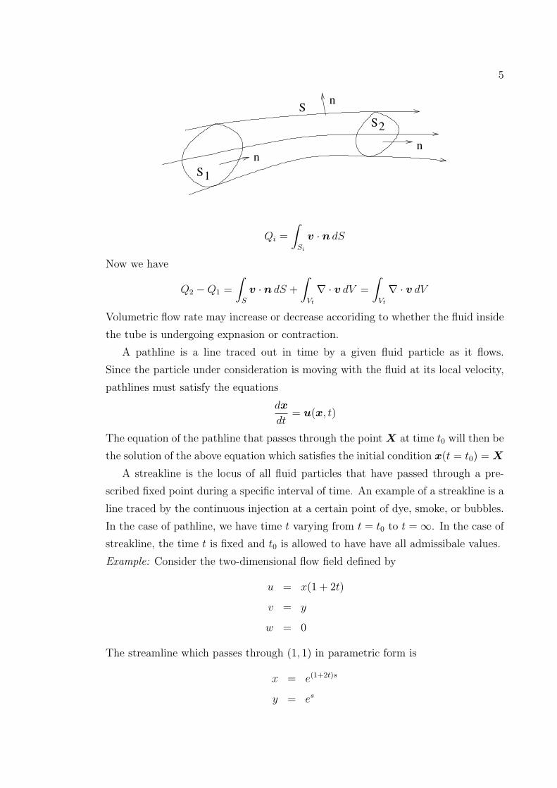
5

nn

S1

S2

Sn

Qi =

∫Si

v · n dS

Now we have

Q2 −Q1 =

∫S

v · n dS +

∫Vt

∇ · v dV =

∫Vt

∇ · v dV

Volumetric flow rate may increase or decrease accoriding to whether the fluid inside

the tube is undergoing expnasion or contraction.

A pathline is a line traced out in time by a given fluid particle as it flows.

Since the particle under consideration is moving with the fluid at its local velocity,

pathlines must satisfy the equations

dx

dt= u(x, t)

The equation of the pathline that passes through the point X at time t0 will then be

the solution of the above equation which satisfies the initial condition x(t = t0) = X

A streakline is the locus of all fluid particles that have passed through a pre-

scribed fixed point during a specific interval of time. An example of a streakline is a

line traced by the continuous injection at a certain point of dye, smoke, or bubbles.

In the case of pathline, we have time t varying from t = t0 to t = ∞. In the case of

streakline, the time t is fixed and t0 is allowed to have have all admissibale values.

Example: Consider the two-dimensional flow field defined by

u = x(1 + 2t)

v = y

w = 0

The streamline which passes through (1, 1) in parametric form is

x = e(1+2t)s

y = es

6

The streamline passing through (1, 1) at t = 0 is

x = es

y = es

or eliminating s we get

x = y

The pathline of the particles passing through (1, 1) at t = 0 is

x = e(1+t)t

y = et

or eliminating t we get

x = y1+log y

The pathline of the particle which is at (1, 1) at t = τ is given by

x = e(1+t)t−τ(1+τ)

y = e(t− τ)

These are parametric equations for streakline that passes through (1, 1) and are

valid for all times t. In particular the streakline at t = 0 in parametric form is

x = e−τ(1+τ)

y = e−τ

or eliminating τ we get

x = y1−log y

Thus none of the three flow lines concide. But if the flow is steady, then they must

concide.

7 Vorticity

We know that the tensor W defined by

W =1

2(L−LT ) or Wij =

1

2(vi,j − vj,i)

is skew symmetric. Hence its dual vector is given by w = (w1, w2, w3) where

wi =1

2εijkvk,j

7

The vorticity ω is twice the dual vetor of W . Hence

ωi = εijkvk,j or ω = ∇∧ v

It is sometimes useful to understand the dynamics of flow by working with the

vorticity rather than the velocity field. Thus we would like to have equation for ω.

The following derivations are based on the incompressible fluid with ν = µ/ρ. The

constant ν is called kinematic viscosity. We have in absence of body forces

∂u

∂t+ (∇u)u = −∇(p/ρ) + ν∇2u

Now we use the following two identities

∇2u = ∇(∇ · u)−∇ ∧ ω

(∇u)u = ∇(|u|2

2

)+ ω ∧ u

Thus we obtained

∂u

∂t+ ω ∧ u = −∇

(|u|2

2+p

ρ

)− ν∇∧ ω

Again taking curl on both sides we get

∂ω

∂t+∇∧ (ω ∧ u) = −ν∇∧ (∇∧ ω)

= ν∇2ω

Again using the identity

∇∧ (a ∧ b) = (∇a)b− (∇b)a + (∇ · b)a− (∇ · a)b

we get∂ω

∂t+ (∇ω)u = ν∇2ω + (∇u)ω

The term ∂ω/∂t represents convection of vorticity with the flow, ν∇2ω represent

diffusion of vorticity and (∇u)ω represenst stretching of the vortex line.

7.1 Vortex lines and vortex tubes

Just as a streamlines is a curve to which the vlocity vector is tangent everywhere,

we can define a vortex line is a curve in which the vorticity is tangent everywhere.

Hence equation is given bydx

ω1

=dy

ω2

=dz

ω3

8

A vortex tube is the series of vortex line passing through a closed curve. Consider

a stream tube with one section of area S1 and the other S2. Since ∇ · ω = 0 and if

Γi =

∫Si

ω · n dS, i = 1, 2

then Γ1 = Γ2. Also using Stoke’s theorem we have

Γi =

∫Si

ω · n dS =

∫Ci

u · dx

where Ci is the curve enclosing Si. The last intergral is the circulation along the

curve.

7.2 Kelvin’s circulation theorem

We can also prove the circulation along a closed curve reamins constant for a ideal

barotropic fluid with conservative body force. For barotropic fluid we have p = p(ρ)

and hence if we define

P =

∫ p dp

ρthen ∇P =

∇pρ

Also for conservative body force we write b = ∇χ. Thus We have

Γ =

∫Ct

v · dx

Using Reynolds circulation theorem we get

dΓ

dt=

∫Ct

[Dv

Dt+ (∇v)T v

]· dx

=

∫Ct

[−1

ρ∇p+∇χ+ (∇v)T v

]· dx

=

∫Ct

∇(P + χ+

vivi

2

)· dx

=

∫Ct

d(P + χ+

vivi

2

)= 0

8 The Stream function

Sometimes it is convenient to describe fluid flow in terms of a stream function,

usually represented by ψ, that remains constant along stream line. The equation of

mass conservation states that

∇ · v = 0

9

We can take v = ∇ ∧A as a genereal solution for this. However A is not unique

since if A′ = A +∇q then

∇∧ a = ∇∧A′

Now the vorticity is

ω = ∇∧ v = ∇∧ (∇∧A) = −∇2A +∇(∇ ·A)

Since A is non unique, we impose the condition that ∇ · v = 0 and thus

ω = −∇2A

Examples

(i) Two dimensional flow : Here v = u(x, y)i + b(x, y)j. If we pick A = ψ(x, y)k

then ∇ ·A = ∂ψ/∂z = 0. Now

v = ∇∧ (ψk) =∂ψ

∂yi− ∂ψ

∂xj

Hence

u =∂ψ

∂yv = −∂ψ

∂x

For two dimensional flow we have ω = −∇2A = −∇2ψk. Hence (∇v)ω = 0. Thus

the vorticity equation becomes

∂∇2ψ

∂t+ (∇∇2ψ)v = ν∇4ψ

Thus the Navier-Stokes equation can be written as

u =∂ψ

∂yv = −∂ψ

∂x

ζ = −∇2ψ∂ζ

∂t+ (∇ζ)v = ν∇2ζ

(ii) Axisymmetric flow : In cylindrical polar coordinate, the velocity is

v = u(r, z)er + w(r, z)ez

Let us choose A = (ψ/r)eθ where ψ = ψ(r, z). Now

∇ ·A =1

r

∂

∂r(rAr) +

1

r

∂Aθ

∂θ+∂Az

∂z=

1

r2

∂ψ

∂θ= 0

10

Thus we can represent fluid velocity as

v = ∇∧A =

(1

r

∂Az

∂θ− ∂Aθ

∂z

)er +

(∂Ar

∂z− ∂Az

∂r

)eθ +

1

r

(∂

∂r(rAθ)−

∂Ar

∂θ

)ez

=1

r

(∂ψ

∂rez −

∂ψ

∂zer

)Thus we get

u = −1

r

∂ψ

∂z, w =

1

r

∂ψ

∂r

Alternatively if we have defined A = ψeθ, where ψ = ψ(r, z), then we obtain

u = −∂ψ∂z, w =

1

r

∂

∂r(rψ)

Thus the stream function can be defined in the equivalent but different ways (ii)

Spherical flow independent of azimuth φ: Here we have

v = u(r, θ)er + w(r, θ)eθ

Let us choose

A =ψ(r, θ)

r sin θeφ

then

∇ ·A =1

r2 sin2 θ

∂ψ(r, θ)

∂φ= 0

Now we have for velocity

v = ∇∧A =1

r2 sin θ

(∂ψ

∂θer − r

∂ψ

∂reθ

)Thus componentwise

u =1

r2 sin θ

∂ψ

∂θ, w = − 1

r sin θ

∂ψ

∂r

8.1 Physical interpretation

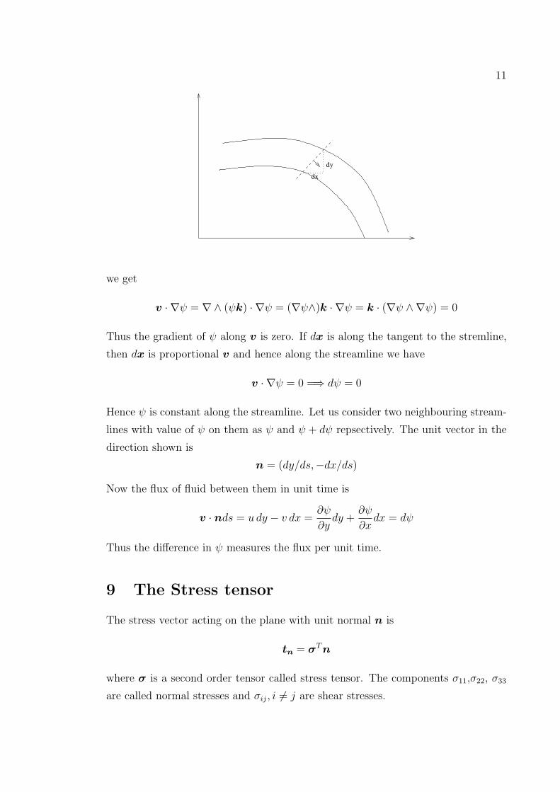
For simplicity we consider two dimensional flow. In this case we have v = ∇∧ (ψk)

Now using the identity

∇∧ (φa) = φ∇∧ a +∇φ ∧ a

11

dx

dy

we get

v · ∇ψ = ∇∧ (ψk) · ∇ψ = (∇ψ∧)k · ∇ψ = k · (∇ψ ∧∇ψ) = 0

Thus the gradient of ψ along v is zero. If dx is along the tangent to the stremline,

then dx is proportional v and hence along the streamline we have

v · ∇ψ = 0 =⇒ dψ = 0

Hence ψ is constant along the streamline. Let us consider two neighbouring stream-

lines with value of ψ on them as ψ and ψ + dψ repsectively. The unit vector in the

direction shown is

n = (dy/ds,−dx/ds)

Now the flux of fluid between them in unit time is

v · nds = u dy − v dx =∂ψ

∂ydy +

∂ψ

∂xdx = dψ

Thus the difference in ψ measures the flux per unit time.

9 The Stress tensor

The stress vector acting on the plane with unit normal n is

tn = σT n

where σ is a second order tensor called stress tensor. The components σ11,σ22, σ33

are called normal stresses and σij, i 6= j are shear stresses.

12

9.1 Stress tensor symmetric

Let Pt ⊂ Bt be an arbitrary material region in the current configuration. The

linear momentum M(Pt) of the material occupying the region Pt in the current

configuration is defined by

M(Pt) =

∫Pt

ρvdv

If x is the position vector of a point in Pt relative origin o, then the angular mo-

mentum of Pt with respect to o is defined by

G(Pt; o) =

∫Pt

x ∧ (ρv)dv

Now applying the conservation of linear momentum for the material in Pt we get

d

dt

∫Pt

ρvdv =

∫Pt

ρbdv +

∫∂Pt

t(n)da,

and applying the conservation of angular momentum we get

d

dt

∫Pt

x ∧ (ρv)dv =

∫Pt

x ∧ (ρb)dv +

∫∂Pt

x ∧ t(n)da,

Using the resultd

dt

∫Pt

ρφdv =

∫Pt

ρDφ

Dtdv

we get ∫Pt

ρ(a− b)dv =

∫∂Pt

t(n)da

and ∫Pt

ρx ∧ (a− b)dv =

∫∂Pt

x ∧ t(n)da,

where a = DvDt

is the acceleration.

From the first relation we get∫Pt

ρ(a− b)dv =

∫∂Pt

σT nda =

∫∂Pt

divσdv

From this we derive

divσ + ρb = ρa

Using this relation in second relation we get∫Pt

x ∧ (divσ)dv =

∫∂Pt

x ∧ (σT n)da

13

Now from the right hand side, we get∫∂Pt

x ∧ (σT n)da =

∫∂Pt

εijkxjσpknpeida

=

∫Pt

εijk (xjσpk),p eidv

=

∫Pt

εijk(δjpσpk + xjσpk,p)eidv

=

∫Pt

[εijkσjkei + εijkxjσpk,pei] dv

=

∫Pt

[εijkσjkei + x ∧ (divσ)] dv

Hence we get ∫Pt

εijkσjkei = 0

From this we get

εijkσjk = 0

Thus taking i = 1, 2, 3 in turn we obtained

σ = σT

9.2 Principal stresses and principal directions

Let σ(x, t) be the stress at a particular point. Let there exists direction n such that

stress vector t(n) = σT n = σn is parallel to n. Thus

σn = σn

The values σ is called principal stresses and the corresponding directions n are called

the principal directions. Also the plane perpendicular to n is called principal stress

plane. Since σ is symmetric, there exists three mutually perpendicular directions

and three principle stresses.

9.3 Cauchy-Stokes decomposition theorem

Let us consider the spatial distribution of velocity v in two neighbouring points x0

and x. Using Taylor series (retaning only linear term and writing dx = x− x0) we

can write

dv = bv(x, t)− x(x0, t) = L dx = D dx + W dx

14

Now let ds be the length of line element between x0 and x. Then

ds2 = dx · dx = F dX · F dX = dX · F T F X

Now

D

Dt(ds2) = dX · D

Dt(F T F )dX

= dX · (F TF + F T F )dX (DP/Dt denoted by P )

= dX · (F T LT F + F T LF )dX

= F dX · (LT + L)F dX

= 2dx ·Ddx

Thus we have1

ds

D ds

Dt= Dij

dxi

ds

dxj

ds= Dijninj

Since D is real and symmetric and therefore has three real eigen values and three

mutually orthogonal eigen vectors. Thus under the action of this term three in-

finitesimal fluid parcels resembling slender needles that are initially aligned with the

eigen vectors will elongate or compress in their respective directions while remaining

orthogonal to each other. Thus a spherical fluid parcels with its three axes aligned

with the eigen vectors will deform (ellipsoidal), increasing or decreasing the the as-

pect ratios while maintaining its original directions. Thus D represents deformation

that preserves parcels orientation. To interpret vorticity, we note that the second

term of can be written as

Ω ∧ dx

where Ω = ω/2. Thus under the action of this term the point particles rotate about

the point x0 with angular velocity that is equal to the half the vorticity of the fluid.

Thus the vorticity vector is parallel to the angular velocity of the point particles

and is equal to the twice the angular velocity of the point particles.

Thus the most general differential motion of a fluid element corresponds to a

uniform translation, plus a rigid rotation plus a distortion.

The following proof shows how a spherical fluid parcel deforms into a ellipsoid Con-

sider a small sphere of radious dr at time t. Let the axis be the principal axes of D.

Let the particles on the sphere of center x is x+n dr where n is a unit vector. The

material coordinate of the center and the point on the spehre are X and X + dX.

Thus

nidr =

(∂xi

∂Xj

)t

dXj

15

In the interval from t to t+ dt the center moves from x(X, t) to x(X, t+ dt). If dy

is the relative position of the of a particle on the surface relative to the center, then

we have

dyi = xi(X + dX, t+ dt)− xi(X, t+ dt) =

(∂xi

∂Xj

)t+dt

dXj

Now (∂xi

∂Xj

)t+dt

=

(∂xi

∂Xj

)t

+ dtD

Dt

(∂xi

∂Xj

)t

=

(∂xi

∂Xj

)t

+ dt

(∂vi

∂Xj

)We can also write the first relation (using inverse mapping) as

dXj =

(∂Xj

∂xk

)t

nkdr

Thus we get

dyi = nidr +

(∂vi

∂Xj

)dXjdt

= nidr +

(∂vi

∂Xj

) (∂Xj

∂xk

)t

nkdrdt

= nidr +

(∂vi

∂xk

)nkdrdt = Aiknkdr

where due to principal axes of D

Aii = 1 +Diidt, i = k no sum

and

Aik =1

2(vi,k − vk,i), i 6= k

The off diagonal term represent rigid rotation. In the absence of rotation we have

since ni are unit vector,

1 =dyi dyi

(1 +Diidt)2dr2

and this is an infinitesimal ellipsoid whose axes are concident with the principal

axes of stretching of length (1 +Diidt)dr, i = 1, 2, 3 (no sum). Thus in the complete

deformation, a small sphere is distorted into an ellipsoid and rotated.

16

10 Constitutive equations

10.1 Stokesian Fluid

A Stokesian fluid satisfies the following assumption

I. The stress tensor is a continuous function of the rate of strain tensor Dij and

local thermodynamic state but independent of other kinematical quantities.

II. The fluid is homogeneous i.e. σij does not depend explicitly on x

III. The fluid is isotropic, i.e. there is no preferred direction.

IV. When there is no deformation (Dij = 0) the stress is hydrostatic i.e. σij =

−pδij

The first assumption implies that relation between stress and strain is independnt of

the rigid body rotation by Wij. The thermodynamic variables, for example, pressure

and temperature, will be carried along throughout the discussion without specific

mention. Due to homogeneous nature the stress tensor depend on position through

the variation of Dij. The third assumption is isotropy and we first show that it

implies that the principal direction of two tensors concide. To express isotropy as

an equation we write σij = fij(Dij), then if there is not preferred direction, we also

have σij = fij(Dij). Let us write

σij = −pδij + τij

where τij is also isotropic and vanish when there is no deformation.

Since τ is isotrpic we must have

τ (QDQT ) = Qτ (D)QT

Choose the coordinate axes as the principal axes of D. Then in this coordinate we

have

[Dij] =

D1 0 0

0 D2 0

0 0 D3

and

τij = τij(D1, D2, D3)

17

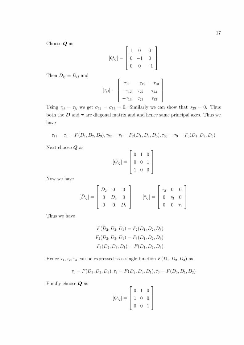
Choose Q as

[Qij] =

1 0 0

0 −1 0

0 0 −1

Then Dij = Dij and

[τij] =

τ11 −τ12 −τ13

−τ12 τ22 τ23

−τ13 τ23 τ33

Using τij = τij we get σ12 = σ13 = 0. Similarly we can show that σ23 = 0. Thus

both the D and τ are diagonal matrix and and hence same principal axes. Thus we

have

τ11 = τ1 = F (D1, D2, D3), τ22 = τ2 = F2(D1, D2, D3), τ33 = τ3 = F3(D1, D2, D3)

Next choose Q as

[Qij] =

0 1 0

0 0 1

1 0 0

Now we have

[Dij] =

D2 0 0

0 D3 0

0 0 D1

[τij] =

τ2 0 0

0 τ3 0

0 0 τ1

Thus we have

F (D2, D3, D1) = F2(D1, D2, D3)

F2(D2, D3, D1) = F3(D1, D2, D3)

F3(D2, D3, D1) = F (D1, D2, D3)

Hence τ1, τ2, τ3 can be expressed as a single function F (D1, D2, D3) as

τ1 = F (D1, D2, D3), τ2 = F (D2, D3, D1), τ3 = F (D3, D1, D2)

Finally choose Q as

[Qij] =

0 1 0

1 0 0

0 0 1

18

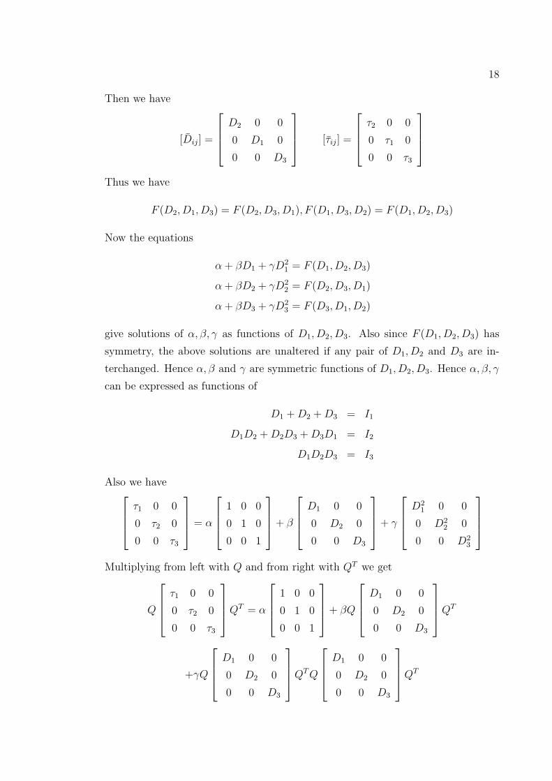
Then we have

[Dij] =

D2 0 0

0 D1 0

0 0 D3

[τij] =

τ2 0 0

0 τ1 0

0 0 τ3

Thus we have

F (D2, D1, D3) = F (D2, D3, D1), F (D1, D3, D2) = F (D1, D2, D3)

Now the equations

α+ βD1 + γD21 = F (D1, D2, D3)

α+ βD2 + γD22 = F (D2, D3, D1)

α+ βD3 + γD23 = F (D3, D1, D2)

give solutions of α, β, γ as functions of D1, D2, D3. Also since F (D1, D2, D3) has

symmetry, the above solutions are unaltered if any pair of D1, D2 and D3 are in-

terchanged. Hence α, β and γ are symmetric functions of D1, D2, D3. Hence α, β, γ

can be expressed as functions of

D1 +D2 +D3 = I1

D1D2 +D2D3 +D3D1 = I2

D1D2D3 = I3

Also we haveτ1 0 0

0 τ2 0

0 0 τ3

= α

1 0 0

0 1 0

0 0 1

+ β

D1 0 0

0 D2 0

0 0 D3

+ γ

D2

1 0 0

0 D22 0

0 0 D23

Multiplying from left with Q and from right with QT we get

Q

τ1 0 0

0 τ2 0

0 0 τ3

QT = α

1 0 0

0 1 0

0 0 1

+ βQ

D1 0 0

0 D2 0

0 0 D3

QT

+γQ

D1 0 0

0 D2 0

0 0 D3

QTQ

D1 0 0

0 D2 0

0 0 D3

QT

19

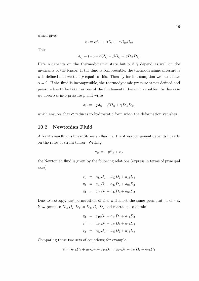
which gives

τij = αδij + βDij + γDikDkj

Thus

σij = (−p+ α)δij + βDij + γDikDkj

Here p depends on the thermodynamic state but α, β, γ depend as well on the

invariants of the tensor. If the fluid is compressible, the thermodynamic pressure is

well defined and we take p equal to this. Then by forth assumption we must have

α = 0. If the fluid is incomprssible, the thermodynamic pressure is not defined and

pressure has to be taken as one of the fundamental dynamic variables. In this case

we absorb α into pressure p and write

σij = −pδij + βDij + γDikDkj

which ensures that σ reduces to hydrostatic form when the deformation vanishes.

10.2 Newtonian Fluid

A Newtonian fluid is linear Stokesian fluid i.e. the stress component depends linearly

on the rates of strain tensor. Writing

σij = −pδij + τij

the Newtonian fluid is given by the following relations (express in terms of principal

axes)

τ1 = a11D1 + a12D2 + a13D3

τ2 = a21D1 + a22D2 + a23D3

τ3 = a31D1 + a32D2 + a33D3

Due to isotropy, any permutation of D’s will affect the same permutation of τ ’s.

Now permute D1, D2, D3 to D3, D1, D2 and rearrange to obtain

τ3 = a12D1 + a13D3 + a11D3

τ1 = a22D1 + a23D2 + a21D3

τ2 = a32D1 + a33D2 + a31D3

Comparing these two sets of equations; for example

τ1 = a11D1 + a12D2 + a13D3 = a22D1 + a23D2 + a21D3

20

gives a11 = a22, a12 = a23, a13 = a21

Doing this for all and for the sets of equation obtain by permuting D1, D2, D3 to

D2, D3, D1 we find

a11 = a22 = a33 = λ+ 2µ

a12 = a21 = a23 = a32 = a13 = a31 = λ

Thus

τi = λ(D1 +D2 +D3) + 2µDi = λtr(D) + 2µDi

Transforming to a general coordinate system we get

τij = λtr(D)δij + 2µDij

Hence

σij = −pδij + λ(∇ · v)δij + 2µDij

11 Fluids

A fundamental characteristic of any fluid is that the action of shear stresses, no

matter how small they might be, will cause the fluid to deform continuously as long

as the shear stresses act. Thus a fluid at rest the stress vector on any plane is normal

to that plane. Thus every plane is a principal plane and consequently every direction

is an eigen vector of the stress tensor. If n1 and n2 are two arbitrary directions and

σ1 and σ2 are two eigen values then

σn1 = σ1n1 and σn2 = σ2n2

Since

n1 · σn2 = n2 · σn1

we get

(σ1 − σ2)n1 · n2 = 0

Since n1 and n2 arbitrary, we have σ1 = σ2 = −p. Hence we write

σ = −pI or σij = −pδij

The sclar p is the magnitude of the compressive normal stress and is known as

hydrostatic pressure.

21

12 Compressible and Incompressible Fluids

We define an incompressible fluid to be the one for which the density of every

particle remains the same at all times regardless of the state of stress. Thus for an

incompressible fluidDρ

Dt= 0

It then follows that

div v = 0

An incompressible fluid need not have a spatially uniform density. If the density is

also uniform, it is referred to as homogeneous fluid for which ρ is constant every-

where.

The compressible fluids are those for which the density change appreciably with

pressure.

13 Equations of hydrostatics

The term hydrostatic refers to the study of fluid at rest i.e. v = 0. Thus with

σij = −pδij the equilibrium equations become

∂p

∂xi

= ρbi or grad p = ρb

In case the only force acting on the body is the force of gravity, then with x3-axis

pointing upwards, we get

∂p

∂x1

= 0

∂p

∂x2

= 0

∂p

∂x3

= −ρg

This shows that the pressure p is independnt of x1 and x2. In case of homeogeneous

fluid i.e. (constant density) we further get

p = −ρgx3 + p0

where p0 is a constant.

22

14 Newtonian fluid

Since the state of stress for a fluid under rigid body motion (including rest) is given

by isotropic, it is natural to decompose the stress tensor into two parts

σij = −pδij + τij

where the values of τij depends on the rate and /or higher rates of deformation

such that they are zero when the fluid is under rigid body motion (i.e. zero rates

of deformation) and p is a scalar whose value does not depend explicitly on these

rates.

We idealized the fluid as a Newtonian fluid if

a. The values of τij at any time t depend linearly on the componenets of rate of

deformation tensor

Dij =1

2(vi,j + vj,i)

at that time and not on any other kinematic quantities.

b. The fluid is isotropic

Following the same argument as the linear isotropic solid we get

τij = λDk,kδij + 2µDij

where λ and µ are called viscosity coefficient.

For a fluid under rigid body motion (i.e. zero rate of deformation) we have

p = −1

3σii,

i.e. pressure is the total compressive normal stress on any plane as well as the mean

of the normal stresses. But in this case we have

−p+ (λ+ 2µ/3)Dkk = −1

3σii

where k = λ + 2µ/3 is known as coefficient of bulk viscosity. It is clear that when

Dij are non zero, p is neither the total compressive normal stress on any plane unless

the viscous componenets happen to be zero as well as is not the mean of the normal

stresses. Thus we can interpret pressure such that −pδij is that part of σij which

does not depend explicitly on the rate of deformation.

23

If we enforce the condition that the pressure is mean of the compressive normal

stresses, we must have

λ = −2µ/3

which is called Stoke’s condition. Thus choosing µ as the only scaler constant we

write

σij = −pδij + 2µ

(Dij −

1

3Dkkδij

)

15 Law of conservation of energy

The law states that the material derivative of kinetic plus internal energies is equal

to the sum of the rate of work of the surface and body forces, plus all other energies

that enter and leave the body per unit time. Other enrgies may include thermal,

electrical, magnetical etc. Here we only cosidered mechanical and thermal ener-

gies. Let e be the specific internal energy or internal energy per unit mass. The

conservation of energy is stated as

D

Dt

∫V

ρ

(e+

1

2vivi

)dv =

∫V

ρbivi dv +

∫S

t(n)i vi dS +

∫V

ρ r dv −∫

S

qini dS

where r is specific rate at which heat is produced by internal sources and q is the

heat flux vector. Now the term on the left hand side can be written as

D

Dt

∫V

ρ

(e+

1

2vivi

)dv

=

∫V

(ρDe

Dt+ viρ

Dvi

Dt

)dv

=

∫V

(ρDe

Dt+ vi(ρbi + σij,j)

)dv

=

∫V

(ρDe

Dt+ ρvibi + (σijvi), j − σijvi,j

)dv

=

∫V

(ρDe

Dt+ ρvibi − σijDij

)dv +

∫S

t(n)i vi dS

Hence we have ∫V

ρDe

Dtdv =

∫V

σijDijdv +

∫V

ρr dv −∫

V

∇ · q dv

Since the volume V is arbitrary we get

ρDe

Dt= σijDij + ρr −∇ · q

24

The term σijDij is called stress power. For Newtonian Viscous fluid we can explicitly

calculate the stress power. We have

σijDij = (−pδij + τij)Dij = −p∇ · v + Φ

where Φ is the dissipation function. The function Φ is positive definite since we have

Φ = 2µ

(Dij −

1

3(∇ · v)δij

)Dij = 2µ

(DijDij −

1

3(∇ · v)2

)= 2µ

(Dij −

1

3(∇ · v)δij

)2

> 0

Alternative form of energy equation is also possible using definition of enthalpy

h = e+p

ρ

We haveDh

Dt=De

Dt+

1

ρ

Dp

Dt− p

ρ2

Dρ

Dt

Thus we have

ρDh

Dt=Dp

Dt+ Φ +∇ · q

We may relate the heat flux to temperature by Fourier’s law as

qi = −κT,i

Then we get

ρDh

Dt=Dp

Dt+ Φ + (κT,i),i

To close the system we use (i) a thermodynamic equation like e = e(T, p), the

simplest being e = cvT or h = cpT and (ii) equation of state p = ρRT

16 Navier Stokes Equation

These equations describe the conservation of mass, momentum and energy. These

are

Dρ

Dt+ ρvk,k = 0

ρDvi

Dt= −p,i + τij,j + ρbi

ρDe

Dt= −pvk,k + Φ + (κT,i),i

25

where

τij = µ

(vi,j + vj,i −

1

3vk,kδij

)Φ = τijDij = τijvi,j

These are supplemented with the thermodynamic relation and equation of state of

a gas

e = e(T, p)

p = ρRT

These gives seven equations in seven unknowns ρ, p, T, vi, e.

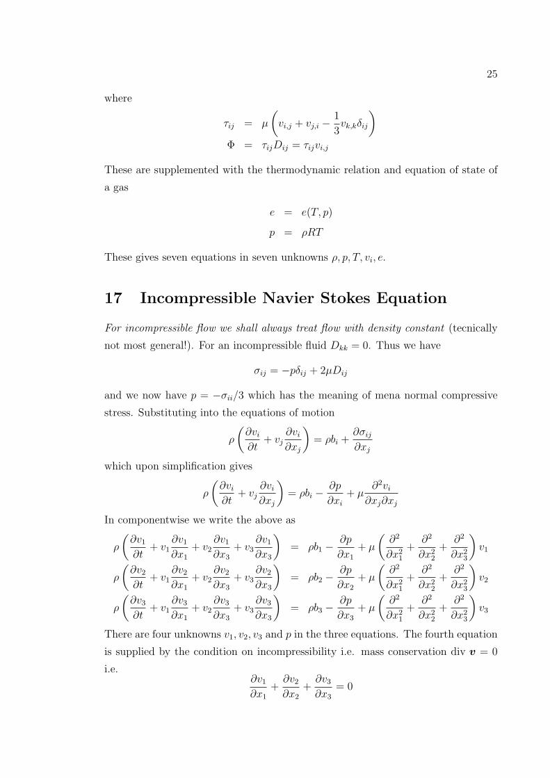
17 Incompressible Navier Stokes Equation

For incompressible flow we shall always treat flow with density constant (tecnically

not most general!). For an incompressible fluid Dkk = 0. Thus we have

σij = −pδij + 2µDij

and we now have p = −σii/3 which has the meaning of mena normal compressive

stress. Substituting into the equations of motion

ρ

(∂vi

∂t+ vj

∂vi

∂xj

)= ρbi +

∂σij

∂xj

which upon simplification gives

ρ

(∂vi

∂t+ vj

∂vi

∂xj

)= ρbi −

∂p

∂xi

+ µ∂2vi

∂xj∂xj

In componentwise we write the above as

ρ

(∂v1

∂t+ v1

∂v1

∂x1

+ v2∂v1

∂x3

+ v3∂v1

∂x3

)= ρb1 −

∂p

∂x1

+ µ

(∂2

∂x21

+∂2

∂x22

+∂2

∂x23

)v1

ρ

(∂v2

∂t+ v1

∂v2

∂x1

+ v2∂v2

∂x3

+ v3∂v2

∂x3

)= ρb2 −

∂p

∂x2

+ µ

(∂2

∂x21

+∂2

∂x22

+∂2

∂x23

)v2

ρ

(∂v3

∂t+ v1

∂v3

∂x1

+ v2∂v3

∂x3

+ v3∂v3

∂x3

)= ρb3 −

∂p

∂x3

+ µ

(∂2

∂x21

+∂2

∂x22

+∂2

∂x23

)v3

There are four unknowns v1, v2, v3 and p in the three equations. The fourth equation

is supplied by the condition on incompressibility i.e. mass conservation div v = 0

i.e.∂v1

∂x1

+∂v2

∂x2

+∂v3

∂x3

= 0

26

These four equations are called Navier Stokes equations of motion for a incompress-

ible fluid. Since the energy equations decouple from the mass conservation and

momentum equations and energy equation need to be solved only when we need

temperarure. For energy equation we have

ρDe

Dt= −pvk,k + Φ + (κT,i),i

Almost always safe to assume that Φ 1. And since the fluid is incompressible we

have (using e = cvT )

ρcvDT

Dt= (κT,i),i

The Navier-Stokes equation in invariant form can be written as

ρ

[∂v

∂t+ (grad v)v

]= ρb− grad p+ µ div (grad v)T

div v = 0

18 Cylindrical coordinate

To derive equations in cylindrical coordinate we need to have the expressions for

gradf , gradv and divA for scalar, vector and tensor fields f,v and A respectively.

Let (r, φ, z) is the cylindrical coordinate with unit base vectors er, eφ, ez. These can

be expressed in terms of cartesian vectors e1, e2, e3 as

er = cosφe1 + sinφe2

eφ = − sinφe1 + cosφe2

ez = e3

From these we get der = dφeφ and deφ = −dφer. From the position vector r =

rer + zez we get

dr = drer + rdφeφ + dzez

18.1 Componennts of gradf

From definition we have

df = (gradf) · dr = [(gradf)rer + (gradf)φeφ + (gradf)zez] · [drer + rdφeφ + dzez]

= (gradf)rdr + (gradf)φrdφ+ (gradf)zdz

27

From calculas

df =∂f

∂rdr +

∂f

∂φdφ+

∂f

∂zdz

Comparing we get

gradf =∂f

∂rer +

1

r

∂f

∂φeφ +

∂f

∂zez

18.2 Components of gradv

We have

v(r, φ, z) = vr(r, φ, z)er + vφ(r, φ, z)eφ + vz(r, φ, z)ez

Fron the definition we have

dv = (gradv)dr = (gradv)(drer + rdφeφ + dzez)

= dr(gradv)er + rdφ(gradv)eφ + dz(gradv)ez

Now

(gradv)er = (gradv)rrer + (gradv)φreφ + (gradv)zrez

(gradv)eφ = (gradv)rφer + (gradv)φφeφ + (gradv)zφez

(gradv)ez = (gradv)rzer + (gradv)φzeφ + (gradv)zzez

Thus

dv = [(gradv)rrer + (gradv)φreφ + (gradv)zrez]dr

+ [(gradv)rφer + (gradv)φφeφ + (gradv)zφez]rdφ

+ [(gradv)rzer + (gradv)φzeφ + (gradv)zzez]dz

Now

dv = dvrer + vrder + dvφeφ + vφdeφ + dvzez

Also from calculas

dvr =∂vr

∂rdr +

∂vr

∂φdφ+

∂vr

∂zdz

dvφ =∂vφ

∂rdr +

∂vφ

∂φdφ+

∂vφ

∂zdz

dvr =∂vz

∂rdr +

∂vz

∂φdφ+

∂vz

∂zdz

28

Using these we get

dv =

[∂vr

∂rdr +

(∂vr

∂φ− vφ

)dφ+

∂vr

∂zdz

]er +

[∂vφ

∂rdr +

(∂vφ

∂φ+ vr

)dφ+

∂vφ

∂zdz

]eφ

+

[∂vz

∂rdr +

∂vz

∂φdφ+

∂vz

∂zdz

]ez

Comparing the above two form we get gradv in matrix form as

[gradv] =

∂vr

∂r

1

r

(∂vr

∂φ− vφ

)∂vr

∂z∂vφ

∂r

1

r

(∂vφ

∂φ+ vr

)∂vφ

∂z∂vz

∂r

1

r

∂vz

∂φ

∂vz

∂z

18.3 divv

Using definiton

divv = tr(gradv) = (gradv)rr + (gradv)φφ + (gradv)zz

=∂vr

∂r+

1

r

(∂vφ

∂φ+ vr

)+∂vz

∂z

18.4 Curl v

The antisymmetric part of gradv in matrix form is

[gradv]A =

0

1

2

(1

r

∂vr

∂φ− vφ

r− ∂vφ

∂r

)1

2

(∂vr

∂z− ∂vz

∂r

)−1

2

(1

r

∂vr

∂φ− vφ

r− ∂vφ

∂r

)0

1

2

(∂vφ

∂z− 1

r

∂vz

∂φ

)−1

2

(∂vr

∂z− ∂vz

∂r

)1

2

(∂vφ

∂z− 1

r

∂vz

∂φ

)0

Since curl is twice the dual vector of antisymmetric part of gradv, we have

Curlv =

(1

r

∂vz

∂φ− ∂vφ

∂z

)er +

(∂vr

∂z− ∂vz

∂r

)eφ +

(vφ

r+∂vφ

∂r− 1

r

∂vr

∂φ

)ez

18.5 Components of divA

We use the identity

div(Av) = (divA) · v + tr(grad(v)A)

29

To get component along er we take v = er. Thus we have

(divA)r = (divA) · er = div(Aer)− tr(grad(er)A)

= div(Arrer + Aφreφ + Azrez)− tr(grad(er)A)

=∂Arr

∂r+

1

r

∂Aφr

∂φ+∂Azr

∂z+Aφφ

r

=∂Arr

∂r+

1

r

∂Aφr

∂φ+∂Azr

∂z+Arr − Aφφ

r

Similarly

(divA)φ =∂Arφ

∂r+

1

r

∂Aφφ

∂φ+∂Azφ

∂z+Aφr + Arφ

r

and

(divA)z =∂Arz

∂r+

1

r

∂Aφz

∂φ+∂Azz

∂z+Arz

r

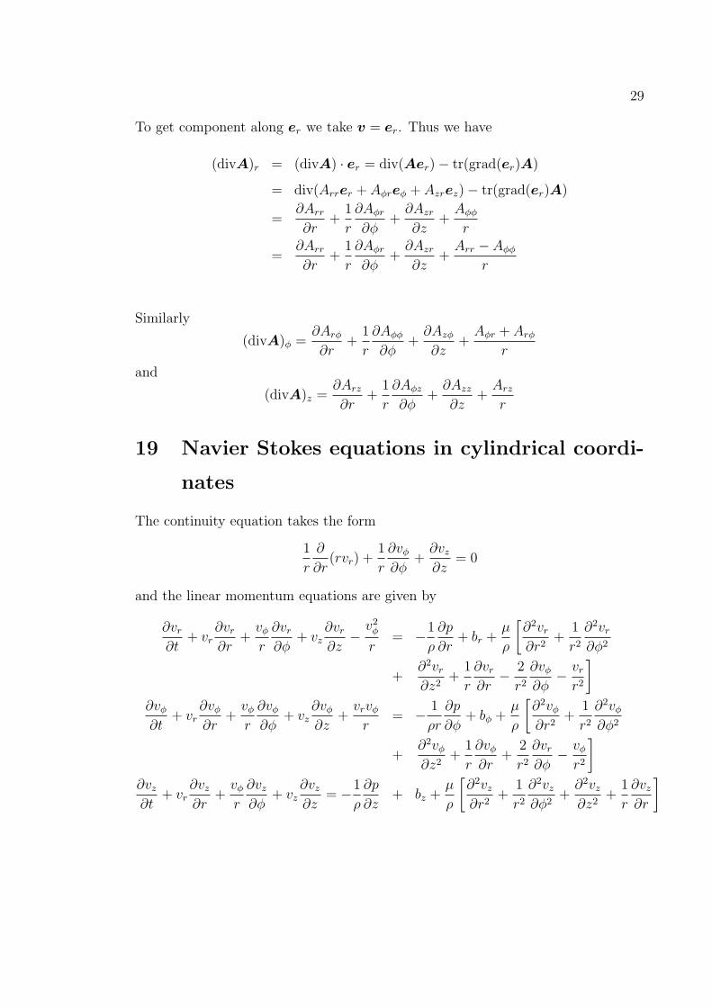
19 Navier Stokes equations in cylindrical coordi-

nates

The continuity equation takes the form

1

r

∂

∂r(rvr) +

1

r

∂vφ

∂φ+∂vz

∂z= 0

and the linear momentum equations are given by

∂vr

∂t+ vr

∂vr

∂r+vφ

r

∂vr

∂φ+ vz

∂vr

∂z−v2

φ

r= −1

ρ

∂p

∂r+ br +

µ

ρ

[∂2vr

∂r2+

1

r2

∂2vr

∂φ2

+∂2vr

∂z2+

1

r

∂vr

∂r− 2

r2

∂vφ

∂φ− vr

r2

]∂vφ

∂t+ vr

∂vφ

∂r+vφ

r

∂vφ

∂φ+ vz

∂vφ

∂z+vrvφ

r= − 1

ρr

∂p

∂φ+ bφ +

µ

ρ

[∂2vφ

∂r2+

1

r2

∂2vφ

∂φ2

+∂2vφ

∂z2+

1

r

∂vφ

∂r+

2

r2

∂vr

∂φ− vφ

r2

]∂vz

∂t+ vr

∂vz

∂r+vφ

r

∂vz

∂φ+ vz

∂vz

∂z= −1

ρ

∂p

∂z+ bz +

µ

ρ

[∂2vz

∂r2+

1

r2

∂2vz

∂φ2+∂2vz

∂z2+

1

r

∂vz

∂r

]

30

20 Navier Stokes equations in spherical coordi-

nates

The continuity equation takes the form

∂vr

∂r+

2vr

r+

1

r

∂vθ

∂θ+

1

r sin θ

∂vφ

∂φ= 0

and the linear momentum equations are given by

∂vr

∂t+ vr

∂vr

∂r+vθ

r

∂vr

∂θ+

vφ

r sin θ∂vr

∂φ−v2θ

r−v2φ

r= −1

ρ

∂p

∂r+ br +

µ

ρ

[∂2vr

∂r2+

1r2∂2vr

∂θ2

+1

r2 sin2 θ

∂2vr

∂φ2+

2r

∂vr

∂r− 2vr

r2+

cot θr2

∂vr

∂θ− 2r2∂vθ

∂θ− 2vθ cot θ

r2− 2r2 sin θ

∂vφ

∂φ

]∂vθ

∂t+ vr

∂vθ

∂r+vθ

r

∂vθ

∂θ+

vφ

r sin θ∂vθ

∂φ+vrvθ

r−v2φ cot θr

= − 1ρr

∂p

∂θ+ bθ +

µ

ρ

[∂2vθ

∂r2

+1r2∂2vθ

∂θ2+

1r2 sin2 θ

∂2vθ

∂φ2+

2r

∂vθ

∂r− vθ

r2 sin2 θ+

cot θr2

∂vθ

∂θ+

2r2∂vr

∂θ− 2 cot θr2 sin θ

∂vφ

∂φ

]∂vφ

∂t+ vr

∂vθ

∂r+vθ

r

∂vφ

∂θ+

vφ

r sin θ∂vφ

∂φ+vrvφ

r+vθvφ cot θ

r= − 1

ρr sin θ∂p

∂φ+ bφ +

µ

ρ

[∂2vφ

∂r2

+1r2∂2vφ

∂θ2+

1r2 sin2 θ

∂2vφ

∂φ2+

2r

∂vφ

∂r−

vφ

r2 sin2 θ+

cot θr2

∂vφ

∂θ+

2r2 sin2 θ

∂vr

∂φ+

2 cot θr2 sin θ

∂vθ

∂φ

]

21 Exact Solutions

21.1 Couette Flow

For steady flow in the absence of body forces the Navier-Stokes equation reduce to

ρ(∇v)v = µ∇ · ((∇v)T )−∇p

∇ · v = 0

Consider the plane velocity field

v(x) = v1(x1, x2)e1

Now the mass conservation implies that

∂v1∂x1

= 0

31

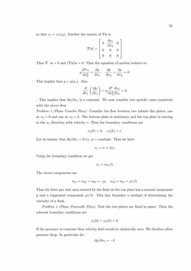
so that v1 = v1(x2). Further the matrix of ∇v is

[∇v] =

0

∂v1∂x2

0

0 0 0

0 0 0

Thus ∇ · v = 0 and (∇v)v = 0. Thus the equation of motion reduces to

µ∂2v1∂x2

2

=∂p

∂x1,

∂p

∂x2=

∂p

∂x3= 0

This implies that p = p(x1). Also

∂

∂x1

(∂p

∂x1

)= µ

∂2

∂x22

∂v1∂x1

= 0

. This implies that ∂p/∂x1 is a constant. We now consider two speicfic cases consistent

with the above flow.

Problem 1 (Plane Couette Flow). Consider the flow between two infinite flat plates, one

at x2 = 0 and one at x2 = h. The bottom plate is stationary and the top plate is moving

in the x1 direction with velocity v. Thus the boundary conditions are

v1(0) = 0, v1(h) = v

Let us assume that ∂p/∂x1 = 0 i.e. p = constant. Thus we have

v1 = α+ βx2

Using the boundary condition we get

v1 = vx2/h

The stress components are

σ11 = σ22 = σ33 = −p, σ12 = σ21 = µv/h

Thus the force per unit area exerted by the fluid on the top plate has a normal component

p and a tangential component µv/h. This fact furnishes a method of determining the

viscosity of a fluid.

Problem 1 (Plane Poiseuille Flow). Now the two plates are fixed in space. Then the

relevent boundary conditions are

v1(0) = v1(h) = 0

If the presuure is constant then velocity field would be identically zero. We therfore allow

pressure drop. In particular let

∂p/∂x1 = −δ

32

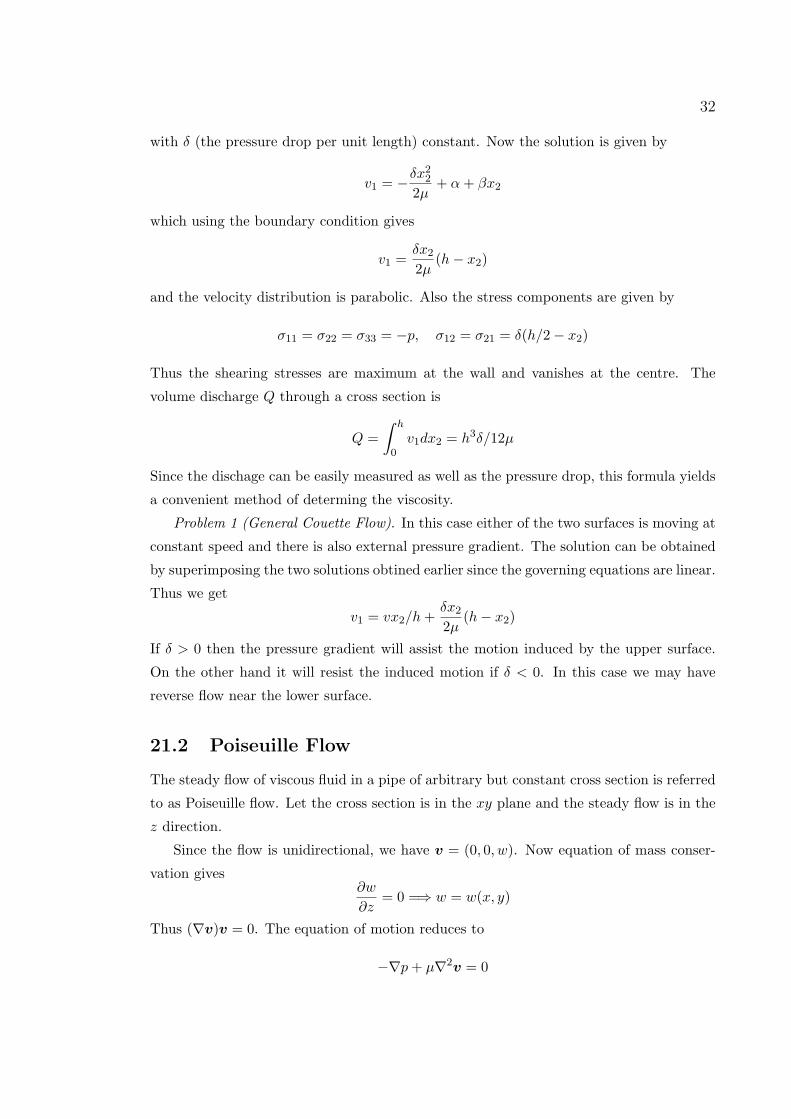
with δ (the pressure drop per unit length) constant. Now the solution is given by

v1 = −δx22

2µ+ α+ βx2

which using the boundary condition gives

v1 =δx2

2µ(h− x2)

and the velocity distribution is parabolic. Also the stress components are given by

σ11 = σ22 = σ33 = −p, σ12 = σ21 = δ(h/2− x2)

Thus the shearing stresses are maximum at the wall and vanishes at the centre. The

volume discharge Q through a cross section is

Q =∫ h

0v1dx2 = h3δ/12µ

Since the dischage can be easily measured as well as the pressure drop, this formula yields

a convenient method of determing the viscosity.

Problem 1 (General Couette Flow). In this case either of the two surfaces is moving at

constant speed and there is also external pressure gradient. The solution can be obtained

by superimposing the two solutions obtined earlier since the governing equations are linear.

Thus we get

v1 = vx2/h+δx2

2µ(h− x2)

If δ > 0 then the pressure gradient will assist the motion induced by the upper surface.

On the other hand it will resist the induced motion if δ < 0. In this case we may have

reverse flow near the lower surface.

21.2 Poiseuille Flow

The steady flow of viscous fluid in a pipe of arbitrary but constant cross section is referred

to as Poiseuille flow. Let the cross section is in the xy plane and the steady flow is in the

z direction.

Since the flow is unidirectional, we have v = (0, 0, w). Now equation of mass conser-

vation gives∂w

∂z= 0 =⇒ w = w(x, y)

Thus (∇v)v = 0. The equation of motion reduces to

−∇p+ µ∇2v = 0

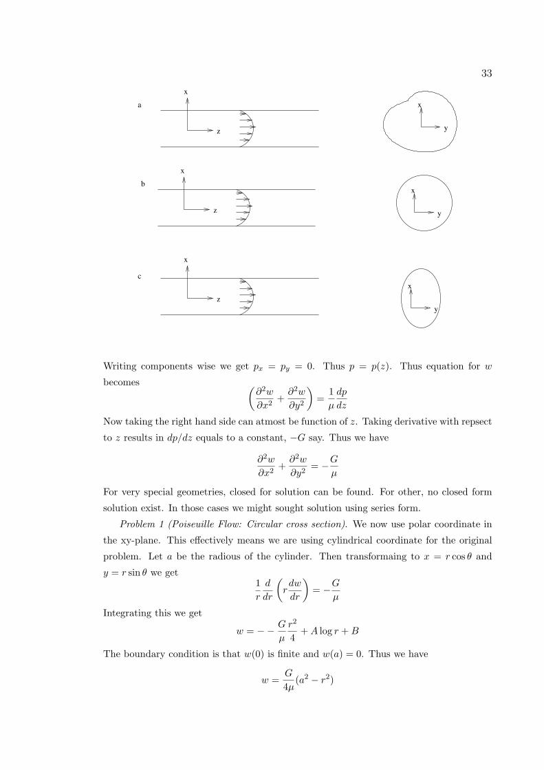
33

z

x

z

x

z

x

y

x

y

x

y

x

a

b

c

Writing components wise we get px = py = 0. Thus p = p(z). Thus equation for w

becomes (∂2w

∂x2+∂2w

∂y2

)=

1µ

dp

dz

Now taking the right hand side can atmost be function of z. Taking derivative with repsect

to z results in dp/dz equals to a constant, −G say. Thus we have

∂2w

∂x2+∂2w

∂y2= −G

µ

For very special geometries, closed for solution can be found. For other, no closed form

solution exist. In those cases we might sought solution using series form.

Problem 1 (Poiseuille Flow: Circular cross section). We now use polar coordinate in

the xy-plane. This effectively means we are using cylindrical coordinate for the original

problem. Let a be the radious of the cylinder. Then transformaing to x = r cos θ and

y = r sin θ we get1r

d

dr

(rdw

dr

)= −G

µ

Integrating this we get

w = −− G

µ

r2

4+A log r +B

The boundary condition is that w(0) is finite and w(a) = 0. Thus we have

w =G

4µ(a2 − r2)

34

The maximum velocity occurs at r = 0 and

wmax =G

4µa2

The same solution could be obtained if we had guessed the solution in the form

w(x, y) = α(x2 + y2 − a2)

Note that this satisfies the boundary condition and the constant α is obtained by substi-

tuting this in the momentum equation for w.

The flux through the pipe is given by

Q =∫ 2π

0

∫ a

0w r dr dθ =

πGa4

8µ

The mean flow velcity is

wav =Flux

Areaofcrosssection=Ga2

8µ

Problem 2 (Poiseuille Flow: Elliptic cross section). Let us assume the axial velocity

of the form

w(x, y) = α

(x2

a2+y2

b2− 1

)It satisfies the boundary condition. Direct substitution into the governing equations for

w gives

α = − G

2µa2b2

a2 + b2

Thus the velocity profile is given by

w(x, y) =G

2µa2b2

a2 + b2

(1−

[x2

a2+y2

b2

])Problem 3 (Poiseuille Flow: Rectangular cross section). Let the flow is confined within

the channel given by −a ≤ x ≤ a and −b ≤ y ≤ b. Thus the equation to be solved is

∂2w

∂x2+∂2w

∂y2= −G

µ

subhject to

w(±a) = w(±b) = 0

We look for solution in the separable form i.e. w(x, y) = X(x)Y (y) withX(±a) = Y (±b) =

0. Hence we choose w as

w(x, y) =∞∑

m=0

∞∑n=0

Amn cos[(2m+ 1)

πx

2a

]cos

[(2n+ 1)

πy

2b

]Where the constants Amn are to be found. These can be found by substituting into the

governing equations for w.

35

21.3 Flow down an inclined plane

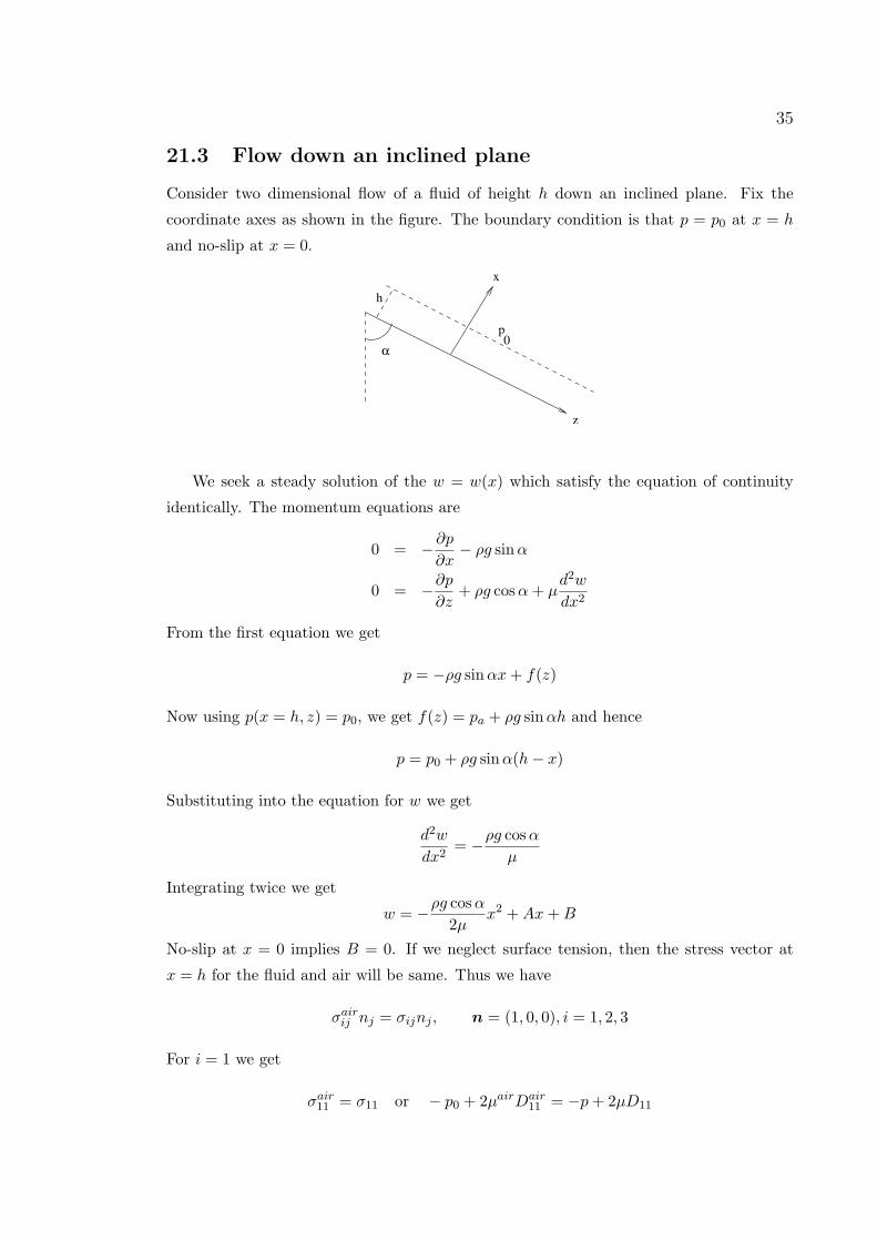
Consider two dimensional flow of a fluid of height h down an inclined plane. Fix the

coordinate axes as shown in the figure. The boundary condition is that p = p0 at x = h

and no-slip at x = 0.

x

z

p0

α

h

We seek a steady solution of the w = w(x) which satisfy the equation of continuity

identically. The momentum equations are

0 = −∂p∂x− ρg sinα

0 = −∂p∂z

+ ρg cosα+ µd2w

dx2

From the first equation we get

p = −ρg sinαx+ f(z)

Now using p(x = h, z) = p0, we get f(z) = pa + ρg sinαh and hence

p = p0 + ρg sinα(h− x)

Substituting into the equation for w we get

d2w

dx2= −ρg cosα

µ

Integrating twice we get

w = −ρg cosα2µ

x2 +Ax+B

No-slip at x = 0 implies B = 0. If we neglect surface tension, then the stress vector at

x = h for the fluid and air will be same. Thus we have

σairij nj = σijnj , n = (1, 0, 0), i = 1, 2, 3

For i = 1 we get

σair11 = σ11 or − p0 + 2µairDair

11 = −p+ 2µD11

36

which is satisfied identically. For i = 2 we get

σair21 = σ21 or 2µairDair

21 = 2µD21

This is also satisfied identically. For i = 3 we have

σair31 = σ31 or 2µairDair

31 = 2µD31

Since µair µ we have at x = h

D31 = 0 ordw

dx= 0 at x = h

This we used to get A and the solution w becomes

w =ρg cosα

2µx(2h− x)

The above solution can be written as

w =ρg cosα

2µ(h2 − (h− x)2)

From this we derive

wmax =ρg cosαh2

2µand Q =

ρg cosαh3

3µ

22 Exact Navier Stokes in cylindrical coordinate

We can make considerbale simplication by assuming that the flow is axisymmetric. This

means that nothing changes with θ thus ∂/∂θ = 0. For an axisymmetric flow with no

swirl we have

v = u(r, z, t)er + w(r, z, t)ez

and for an axisymmetric flow with swirl we have

v = u(r, z, t)er + v(r, z, t)eθ + w(r, z, t)ez

Problem (Steady axisymmetric swirl flow between coaxial cylinder). Fluid fills the annular

gap between two infinitely long coaxial cylinder. The angular velocity of the inner/outer

cylinders of radii a and b are Ω1 and Ω2 respectively. Since the swirl flow is steady and

the cylinders are infiniely long we have

v = v(r)eθ

The equation of continuity is automatically satisfied. The equations of motion are

−v2

r= −1

ρ

dp

dr

0 =d2v

dr2+

1r

dv

dr− v

r2

37

Solving for v gives

v = Ar +B/r

The boundary conditions are v = aΩ1 at r = a and v = bΩ2 at r = b. Using these we get

A =b2Ω2 − a2Ω1

b2 − a2b = a2b2

Ω2 − Ω1

a2 − b2

We also have for vorticity

ω = ∇∧ v = 2b2Ω2 − a2Ω1

b2 − a2ez

and is therefore constant. Now let us calculate the torque on the inner cylinder. To do

this first we calculate the Dθr which using the matrix of ∇v we get

Dθr = −Br2

Hence we get

σθr = −2µB/r2

Now n = er and we have

tn = σer = σrrer + σθreθ + σzrez

We are interested horizonal torque per unit vertical length. This will be given by azimulthal

component σθr. Now for the inner cylinder this torque is given by

τa =∫ 2π

0(a σθr|r=a) a dθ = −4πµB

Substituting the value of a we get

τa = −4πµa2b2Ω2 − Ω1

b2 − a2

Similar calculation for the outer cylinder gives

τb = −4πµa2b2Ω2 − Ω1

b2 − a2

Special cases

Equal rotation rate: In this case the Ω1 = Ω2 and in this case we have

v = Ω1r

Thus the fluid swirls as if it is a rotating rigid body and the couple on both the

cylinder vanish.

38

No inner cylinder: In this case a = 0 and we must have B = 0 to remove the

singularity. Again we have just a rigid body rotation

v = rΩ2

Stationary outer cylinder: We have Ω2 = 0 and we have

v

r=

a2Ω1

b2 − a2

(b2

r2− 1

)Letting b→∞ we get

v =a2Ω1

r

23 Unsteady unidirectional flow

For unsteady unidirectional flow we have to solve

v = we3, w = w(x, y, t),∂v

∂t= −∇p

ρ+ ν∇2v

As in the steady cases, we have

∂p

∂x=∂p

∂y= 0 =⇒ p = p(z, t)

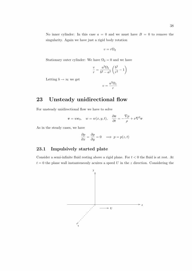
23.1 Impulsively started plate

Consider a semi-infinite fluid resting above a rigid plane. For t < 0 the fluid is at rest. At

t = 0 the plane wall instanteneouly acuires a speed U in the z direction. Considering the

z

y

x

U

39

figure, it is clear that the flow variables must be independent of x and hence w = w(y, t).

Now the momentum equation along z direction gives

ρ∂w

∂t= −∂p

∂z+ µ

∂2w

∂y2

Now the above equation implying ∂p/∂z must be independent of z. Thus we have

p(y, z, t) = p0(y, t) + p1(y, t)z

Since pressure is boundend at z = ±∞ we must have p1(y, t) = 0 and hence ∂p/∂z = 0

Hence the equation reduces to∂w

∂t= ν

∂2w

∂y2

subject to the initial and boundary conditions

w(0, t) = U

w(y, t) → 0 as y →∞

w(y, 0) = 0

We get rid of the constant U by defining W = Uw thus reducing the problem to

∂W

∂t= ν

∂2W

∂y2

subject to the initial and boundary conditions

W (0, t) = 1

W (y, t) → 0 as y →∞

W (y, 0) = 0

Clearly we must have W = φ(ν, y, t).

Solution by Laplace transform: Taking Laplace transform on both sides we get

sW = νd2W

∂y2

subject to

W (0, s) =1s

W (y, s) → 0 as y →∞

The solution is

W = Aey√

s/ν +Be−y√

s/ν

40

Using the boundary conditions we get

W =e−y√

s/ν

s

The inverse transform gives

W (y, t) = erfc(η), where η =y

2√νt

where erfc(η) is defined by

erfc(η) = 1− 2√π

∫ η

0e−t2 dt = 1− erf(η)

Thus the solution is given by

u = U erfc(η), η =y

2√νt

Solution by Similarity: Since W is nondimensional and W = φ(y, ν, t), the function φ

must also be nondimensional. Since y, ν, t involve two independent dimension [L] and [T ]

only one independent nondimensional variable is possible. Let us take the nondimensional

variable as

η =y

2√νt

Thus let us choose

W = f(η)

Putting into the governing equations we have

f′′

= −2ηf′

The boundary conditions are

f(∞) = 0 f(0) = 1

We solve the above as

f ′ = Ae−η2

Integrating once again we get

f = B +A

∫ η

0e−η2

dη

Putting into boundary conditions we get B = 1 and A = −2/√π. Thus we have the same

solution.

41

If we plot the u/U versus η then we observe that u/U = 0.05 at η ≈ 1.4. Thus the

width of the boundary layer δ ≈ 2.8√νt. Thus the boundary layer (see later in the course)

increases as√t. The vorticity is given by

ω = ∇∧ v = − U

π√νte−

y2

4νt e1

Using Gamma function we can show that∫ ∞

0ω dy

is a constant vector for t > 0. Thus there is no new vorticity generated in the flow. The

vorticity at t = 0 due to impulsive start is simply diffuse away with time. And the voritcity

at time t is confined within the layer [0, 2√νt].

23.2 Oscillating flows

Consider the flow similar to the above but the plate is now oscillating with frequency ω.

The governing equations are∂w

∂t= ν

∂2w

∂y2

subject to the boundary conditions

w(0, t) = U cos(ωt)

w(y, t) → 0 as y →∞

We can remove the dependence on U by defining w = UW . Thus reduces the problem to

∂W

∂t= ν

∂2W

∂y2

subject to the boundary conditions

W (0, t) = cos(ωt)

W (y, t) → 0 as y →∞

Note that here W = φ(ν, y, t, ω) and φ must be function of two independent nondimen-

sional variable. Thus similarity solution is not possible. Since the frquency of the wall is

ω and the problem is linear, we assume that the frequency of the fluid flow w is also ω.

To solve let us assume that

W = Re(f(y)eiωt)

Substituting into the governing equations we get

f ′′ =iω

νf

42

subject to the boundary conditions

f(0) = 1 and f(y) → 0 as y →∞

Thus we have

f = Aeλy +Be−λy, λ =

√iω

ν

Now√i = (1 + i)/sqrt2 we must have A = 0. Using the other conditions gives B = 1.

Thus we have

f = e−√

ω/2ν(1+i)y

Hence

w = Ue−√

ω/2νy cos(ωt−

√ω/2νy

)The vorticity is given by

ω = ∇∧ v =∂w

∂ye1 = −U

√ω/νe−

√ω/2νy cos

(ωt−

√ω/2νy + π/4

)e1

Thus most of the vorticity is confined withing the a region of thickness√ν/ω. The higher

the frquence the thinner the layer. The wall shear stress is proportinal to

∂w

∂y

∣∣∣∣y=0

∝ cos(ωt)− sin(ωt) =√

2 cos(ωt+ π/4)

Thus there is a phase difference of π/4 between the wall velocity and wall shear.

24 Stagnation point flow

x

y

Consider the flow of a viscous fluid towards the wall as shown in the figure. Introducing

stream function we can write

u =∂ψ

∂y, v = −∂ψ

∂x

43

If we considered the fluid to be inviscid and irrotatinal, then the governing equations for

ψ is given by

∇2ψ = 0

subject to zero normal velocity at y = 0 i.e. v = 0 at y = 0 or equivalently ψ = 0 at y = 0.

The solution is

ψ = kxy

where k is a constant. Hence

u = kx, v = −ky

Clearly this equation do not satisfy the noslip condition at y = 0. Hence let us assume

solution of the inviscid form as

v = −f(y), u = xf ′(y)

This implies that f ′ → k as y → ∞. With this choice the mass conservation equation is

satisfied automatically. Now consider the y−momentum equation first. Putting the values

of u and v we get

py = −ρ(ff ′ + f ′′) = Q(y)

Hence

p = p(x) +R(y)

From the x−momentum equation we get

px = ρx(νf ′′′ + ff ′′ − f ′2)

Thus

p =ρx2

2(νf ′′′ + ff ′′ − f ′2) + S(y)

The two form for p implies that

νf ′′′ + ff ′′ − f ′2 = β

where β is a constant. Taking y → ∞ we get β = −k2. Also the boundary conditions at

y = 0 becomes f(0) = f ′(0) = 0. Thus the complete problem is given by

νf ′′′ + ff ′′ + k2 − f ′2 = 0

subject to

f(0) = f ′(0) = 0 at y = 0, f ′ → k as y →∞

The solution for the flow must be found numerically.