1 Enviromatics 2008 - Environmental data analysis Environmental data analysis Вонр. проф. д-р Александар Маркоски Технички факултет –

1Enviromatics 2008 - Environmental data analysis

Environmental data analysis

Вонр. проф. д-р Александар Маркоски

Технички факултет – Битола

2008 год.


Introduction

• Applications of data analysis methods are helpful to form a base for environmental modelling and simulation as well as for decision making and environmental impact assessment.

• Disturbances of data analysis are caused by small sets of representative regular sampled data which are available. The power of external and internal driving forces on environmental indicators influences the quality of data to be obtained. The a-priori process information on environmental indicators is low.

• Re-sampling of data can be done by interpolation or approximation methods to place data on a regular time and space grid. Interpolation methods deliver equidistant data while functional relationships result from approximations.


Scales of operation of environmental data• Nominal scale: Pie charts, no arithmetic operation possible,

sometimes coded by numbers.• Ordinal scale: Ranking of events or representations, classification of

environmental indicators (e.g. EU water quality classes, soil classes), ordinal comparisons are possible: Class I > Class II, estimation of median and quartiles.

• Interval scale: Ordinal scale with equal intervals (e.g. temperature), statements on distances and differences between data are allowable. No “natural” origin (zero point) exists.

• Ratio scale: It is an interval scale with a “natural” origin and allows statements on ratios (e.g. concentrations).

• Scale transformations from one data scale to another serve as unifications of variables. The information content and the scale level shall not be changed. If there is no empiric equivalence scale, the data are valuated as “comparable”.


Re-sampling of environmental data

• How to handle missing environmental data? Mostly, series of measurements of environmental data are time series of data recorded at discrete points in time with variable intervals. The goal should be mapping of time series on a regular time grid.

• Re-sampling generally requires a data interpolation or, in the case of noisy information, a data approximation. The goal of the application of interpolation and approximation methods on incomplete time series is to fill the intervals between two grid points so that series of measurements with small intervals are kept.

• If data series contain missing values, then the following procedures are usefully:

1. Filling of gaps with the help of interpolation.

2. Generating of values with the help of approximation functions.

3. Filling of gaps with values of reference curves (analytical or stochastically functions).


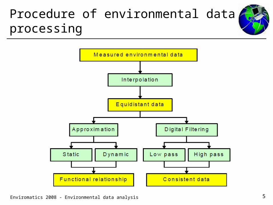
Procedure of environmental data processing


Filling missing data

• In the case of missing data the gaps should be filled in by “artificial” data. Missing data can be estimated by interpolation methods, approximation procedures or data from reference relationships.

• In each case, the data should be placed on a regular time grid with constant observation (sampling) intervals. Only such data should be used for statistics, modelling, simulation and optimisation.

• Otherwise, misinterpretations and incorrect simulation results will be getting. Such results are not suitable for environmental management.


Types of environmental data series


Types of data series

• Type 1: Average is time dependent, dispersion is approximately time constant.

• Type 2: Average is approximately time constant, dispersion is time dependent.

• Type 3: Average and dispersion are time dependent.


Interpolating environmental data


Interpolation of two-weekly water quality data


Comparison of the goodness of different interpolation methods


Approximation of environmental data

• Approximation of ecological signals means that given or estimated functions exist which are able to reproduce sampled environmental data. It can be seen from figure 4 where the following polynomial was computed:

NO3-N(t) = 1,8987 – 0,0754 t + 0,0028 t² - 0,00003 t³


Trend estimation of environmental data

• Linear trend y(t) = a0 (t) + a1 (t) x(t).

• Quadratic trends y(t) = a0 (t) + a1 (t) x(t) + a2 (t) x2 (t).

• Polynomial trend:y(t) = a0 (t) + a1 (t) x(t) + a2 (t) x2 (t) + ..... + an (t) xn (t).

• Exponential trend:x(t) = x(0) e - kt + E.


Environmental data analysis

The End

Documents

1 Enviromatics 2008 - Environmental data analysis Environmental data analysis Вонр. проф. д-р Александар Маркоски Технички факултет –