1 Fiber Textures: application to thin film textures 27-750, Spring 2007 A. D. (Tony) Rollett, A. Gungor & K. Barmak Acknowledgement: the data for these

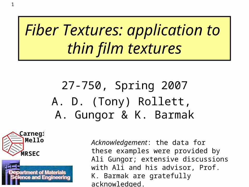
1

Fiber Textures: application to thin film textures

27-750, Spring 2007

A. D. (Tony) Rollett, A. Gungor & K. Barmak

Carnegie Mellon

MRSEC

Acknowledgement: the data for these examples were provided by Ali Gungor; extensive discussions with Ali and his advisor, Prof. K. Barmak are gratefully acknowledged.

2

Example 1: Interconnect Lifetimes

• Thin (1 µm or less) metallic lines used in microcircuitry to connect one part of a circuit with another.

• Current densities (~106 A.cm-2) are very high so that electromigration produces significant mass transport.

• Failure by void accumulation often associated with grain boundaries

Electromigration Weak Strong IPF VolumeFraction PolePlot Deconvolution

3

SiO2W

linerSiNx

ILD via

Inter-Level-Dielectric

M2

Si substrate

SiO2

M1ILD

Silicide Silicide

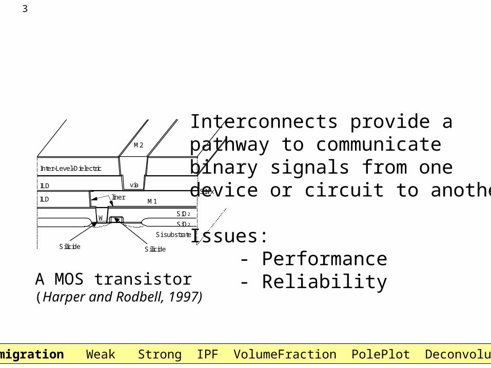
A MOS transistor (Harper and Rodbell, 1997)

Interconnects provide apathway to communicatebinary signals from onedevice or circuit to another.

Issues:- Performance- Reliability


4

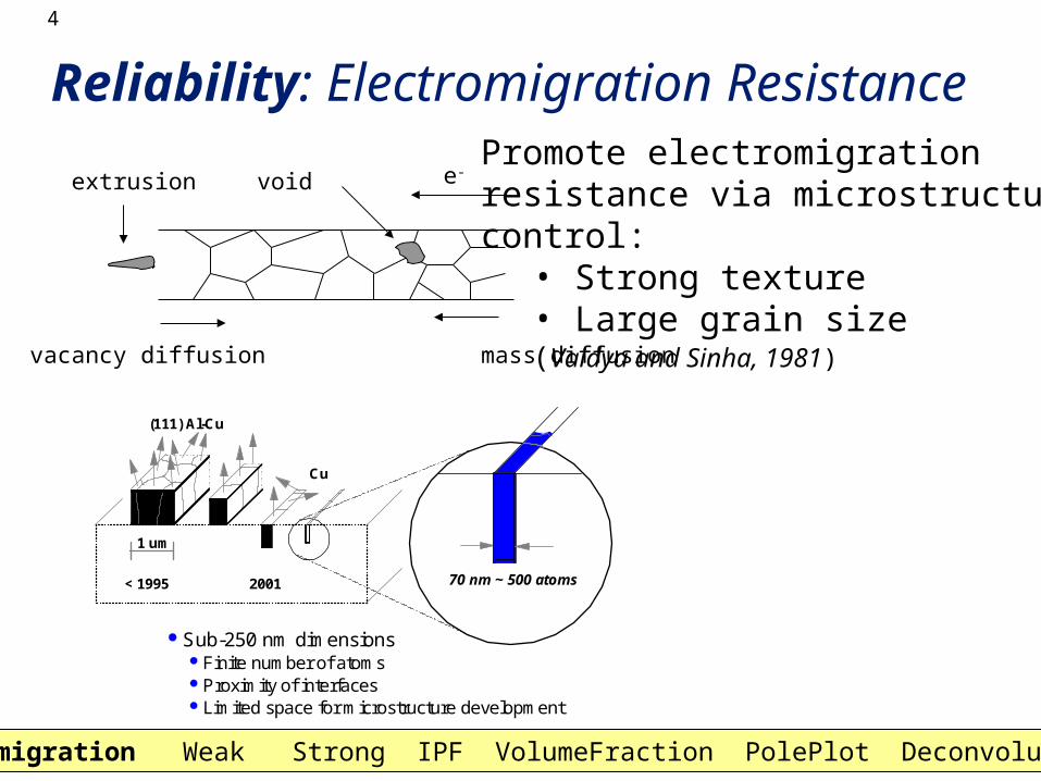
e-extrusion void

vacancy diffusion mass diffusion

Promote electromigrationresistance via microstructurecontrol:

• Strong texture• Large grain size(Vaidya and Sinha, 1981)

1 um

< 1995 2001

(111) Al-Cu

Cu

70 nm ~ 500 atoms

Sub-250 nm dimensionsFinite number of atomsProximity of interfacesLimited space for microstructure development

Reliability: Electromigration Resistance


5

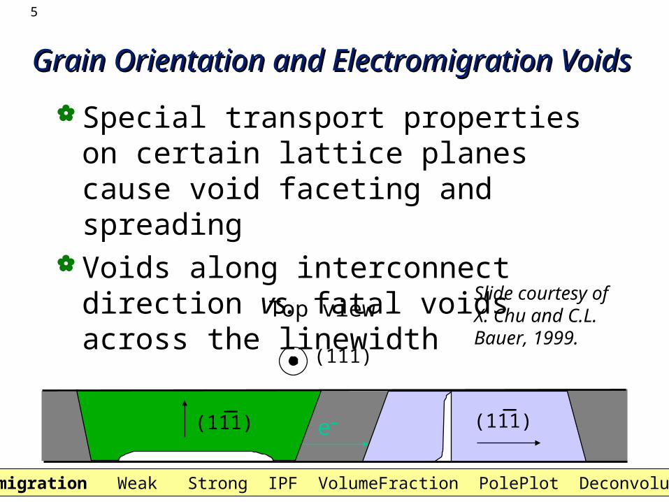
Special transport properties on certain lattice planes cause void faceting and spreading

Voids along interconnect direction vs. fatal voids across the linewidth

Grain Orientation and Electromigration VoidsGrain Orientation and Electromigration Voids

(111)

Top view

(111)_

(111)_

e-


Slide courtesy of X. Chu and C.L. Bauer, 1999.

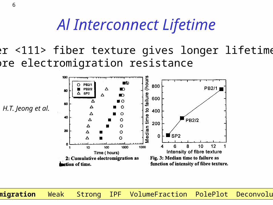
6

Al Interconnect Lifetime

H.T. Jeong et al.

Stronger <111> fiber texture gives longer lifetime, i.e. more electromigration resistance


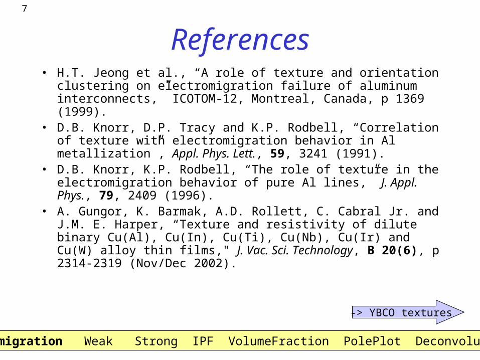
7

References• H.T. Jeong et al., “A role of texture and orientation

clustering on electromigration failure of aluminum interconnects,” ICOTOM-12, Montreal, Canada, p 1369 (1999).

• D.B. Knorr, D.P. Tracy and K.P. Rodbell, “Correlation of texture with electromigration behavior in Al metallization”, Appl. Phys. Lett., 59, 3241 (1991).

• D.B. Knorr, K.P. Rodbell, “The role of texture in the electromigration behavior of pure Al lines,” J. Appl. Phys., 79, 2409 (1996).

• A. Gungor, K. Barmak, A.D. Rollett, C. Cabral Jr. and J.M. E. Harper, “Texture and resistivity of dilute binary Cu(Al), Cu(In), Cu(Ti), Cu(Nb), Cu(Ir) and Cu(W) alloy thin films," J. Vac. Sci. Technology, B 20(6), p 2314-2319 (Nov/Dec 2002).


-> YBCO textures

8

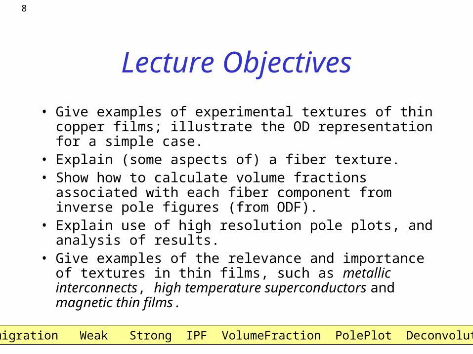
Lecture Objectives

• Give examples of experimental textures of thin copper films; illustrate the OD representation for a simple case.

• Explain (some aspects of) a fiber texture.• Show how to calculate volume fractions associated with

each fiber component from inverse pole figures (from ODF).

• Explain use of high resolution pole plots, and analysis of results.

• Give examples of the relevance and importance of textures in thin films, such as metallic interconnects, high temperature superconductors and magnetic thin films.


9

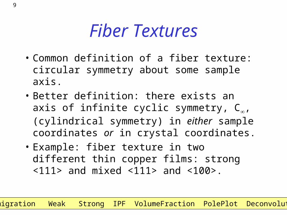
Fiber Textures

• Common definition of a fiber texture: circular symmetry about some sample axis.

• Better definition: there exists an axis of infinite cyclic symmetry, C, (cylindrical symmetry) in either sample coordinates or in crystal coordinates.

• Example: fiber texture in two different thin copper films: strong <111> and mixed <111> and <100>.


10

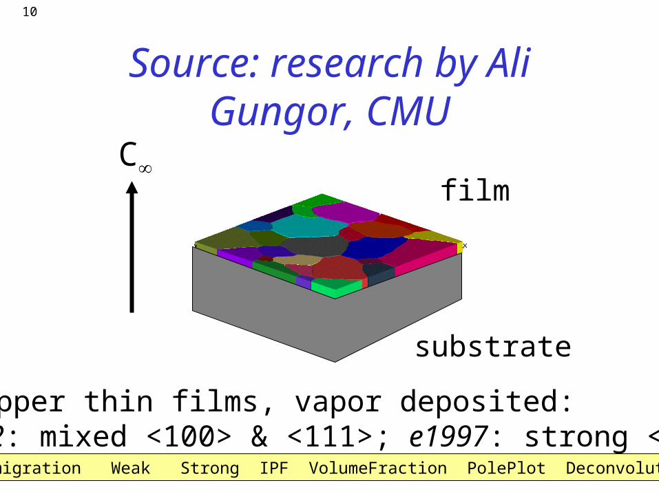
Source: research by Ali Gungor, CMU

substrate

filmC

2 copper thin films, vapor deposited:e1992: mixed <100> & <111>; e1997: strong <111>


11

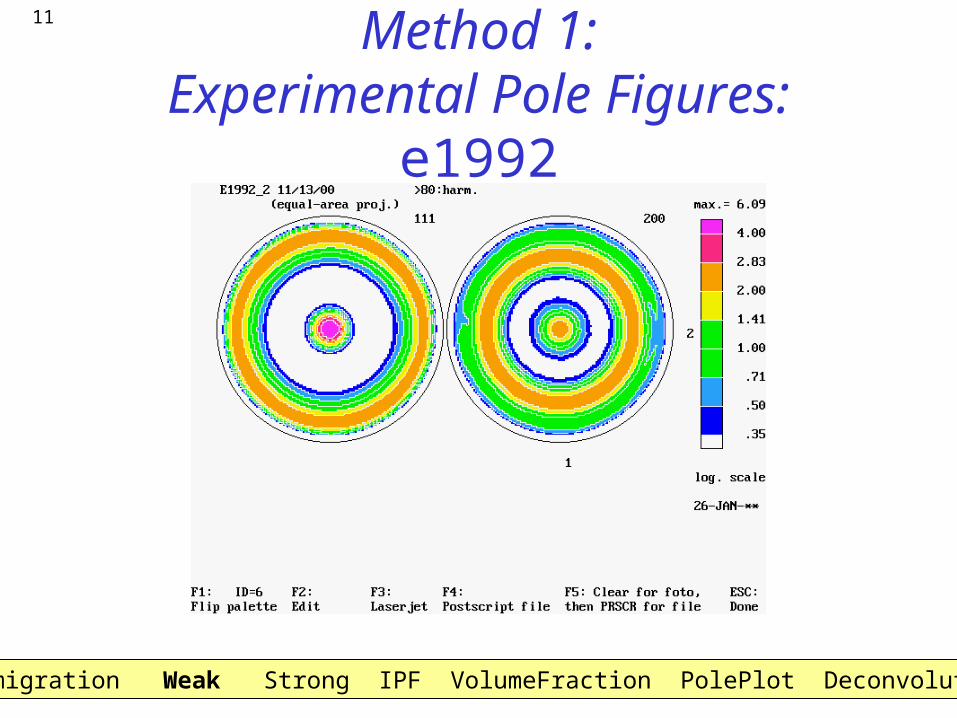
Method 1:Experimental Pole Figures: e1992


12

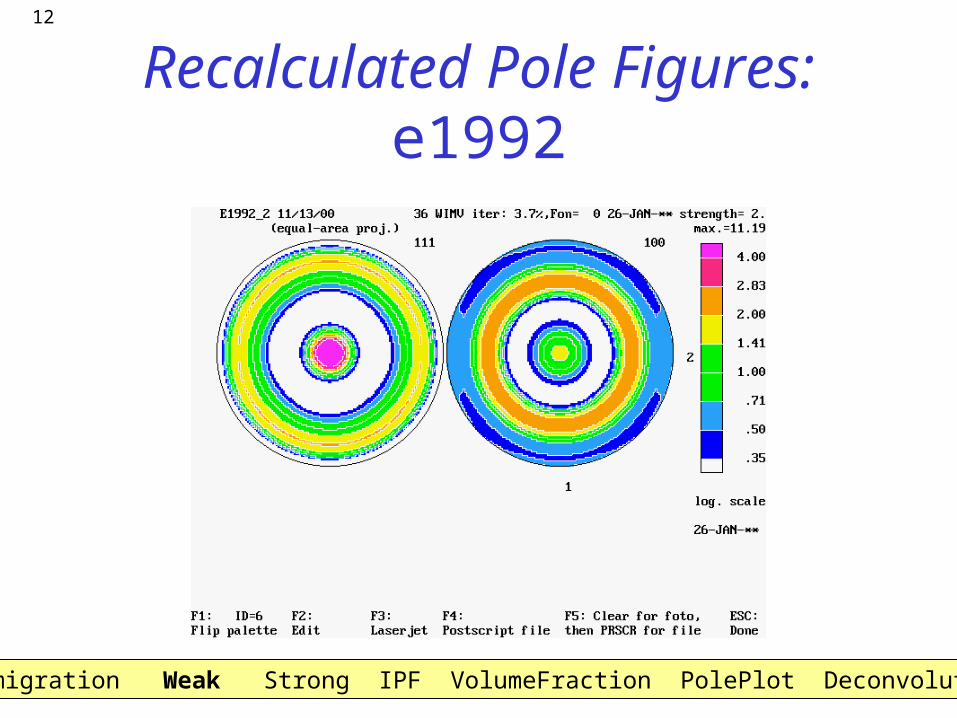
Recalculated Pole Figures: e1992


13

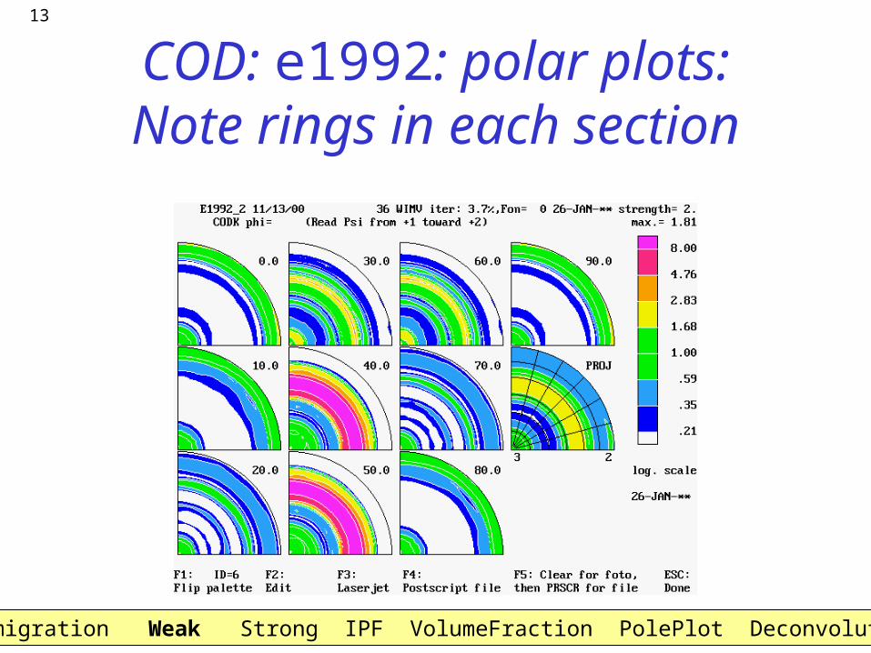
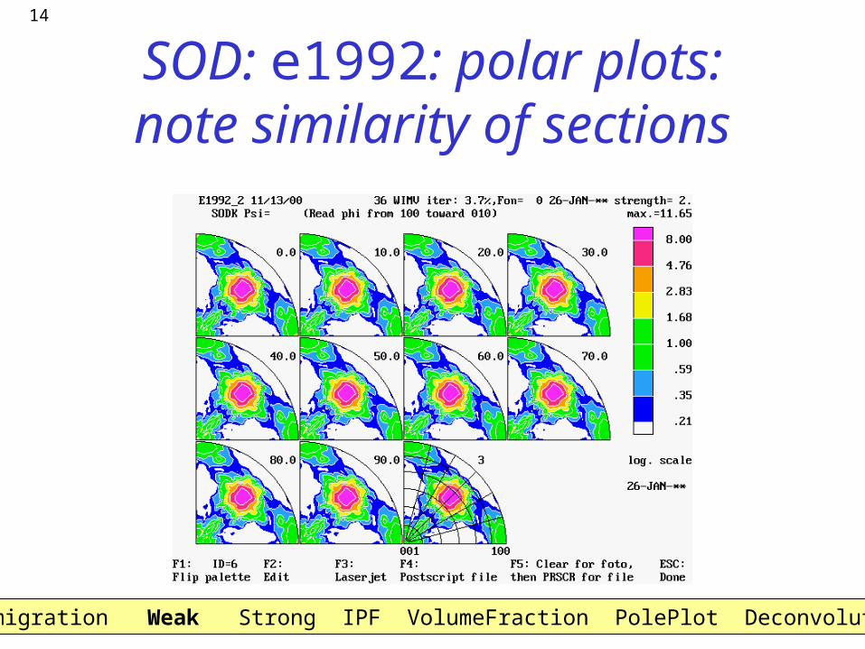
COD: e1992: polar plots:Note rings in each section


14

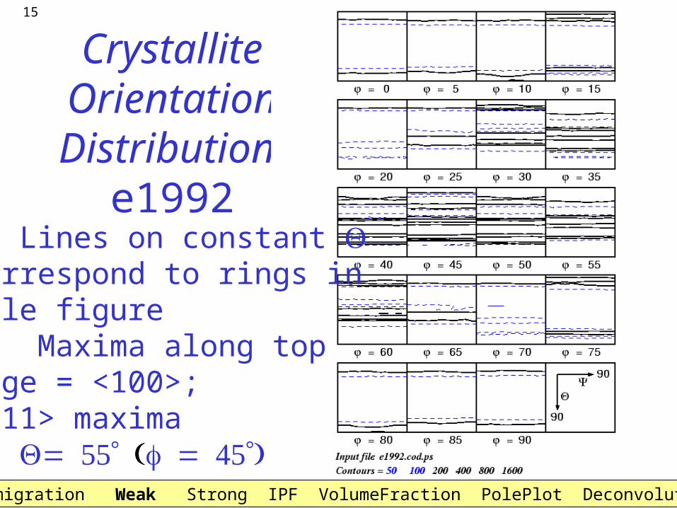
SOD: e1992: polar plots:note similarity of sections


15

Crystallite Orientation

Distribution:e1992

1. Lines on constant correspond to rings inpole figure2. Maxima along top edge = <100>;<111> maxima on Electromigration Weak Strong IPF VolumeFraction PolePlot Deconvolution

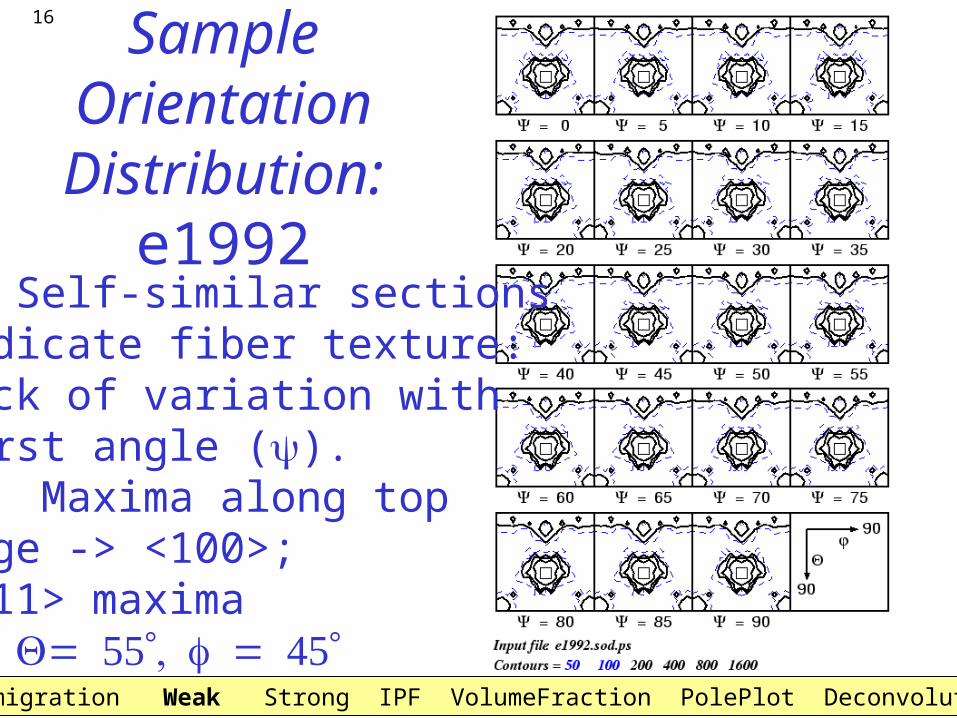
16 Sample Orientation

Distribution: e1992

1. Self-similar sectionsindicate fiber texture:lack of variation withfirst angle ().2. Maxima along top edge -> <100>;<111> maxima on Electromigration Weak Strong IPF VolumeFraction PolePlot Deconvolution

17

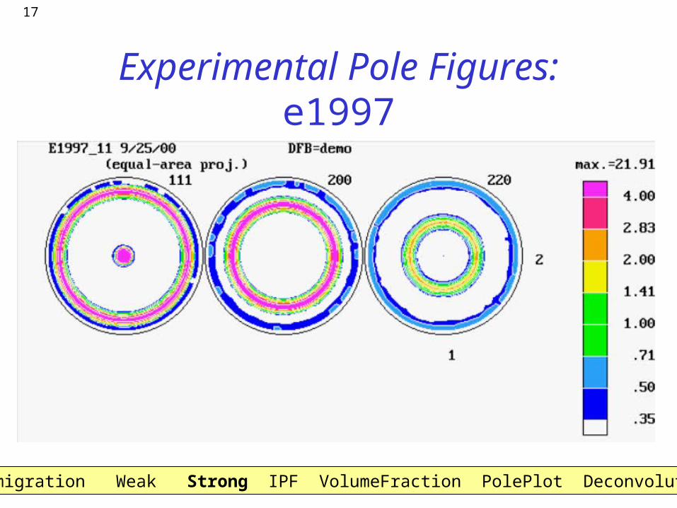
Experimental Pole Figures: e1997


18

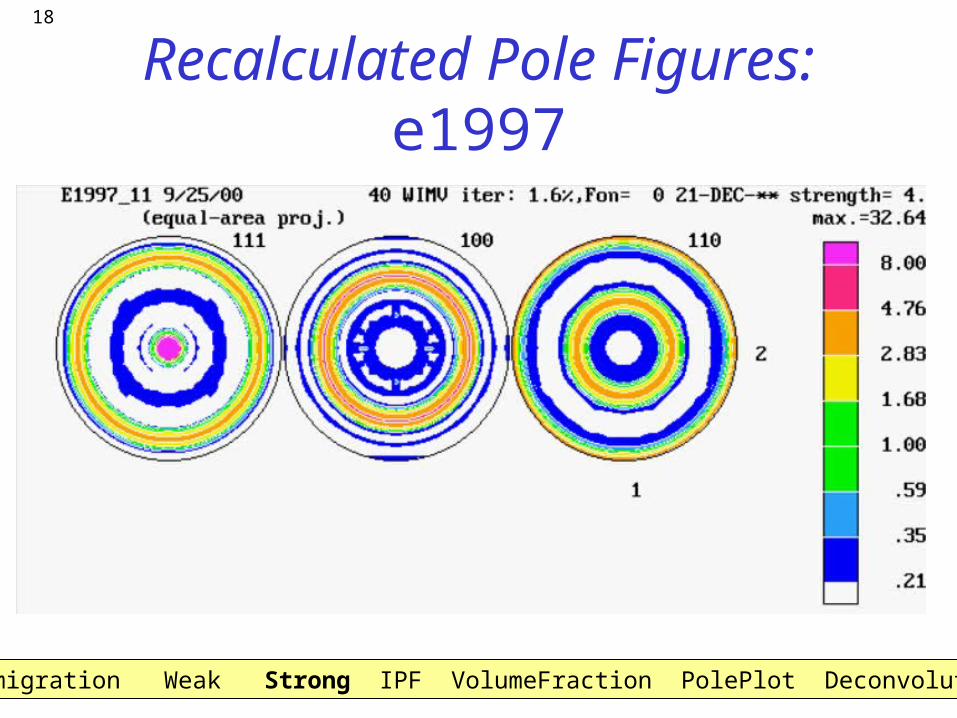
Recalculated Pole Figures: e1997


19

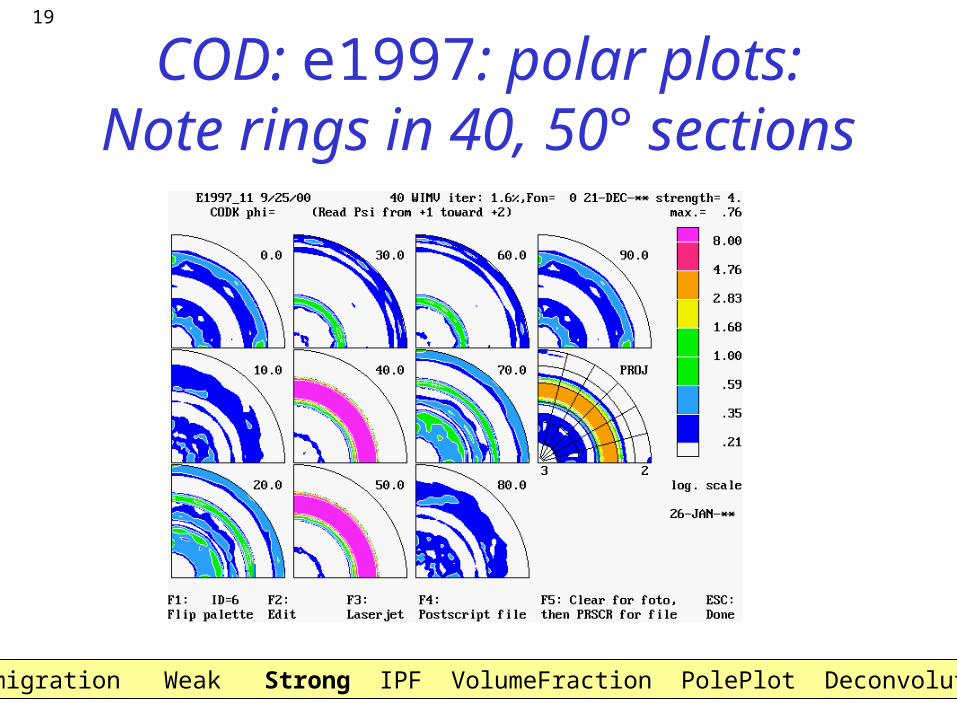
COD: e1997: polar plots:Note rings in 40, 50° sections


20

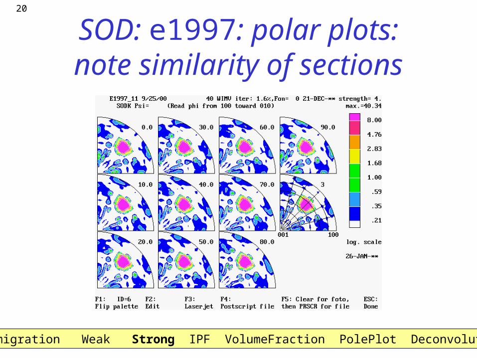
SOD: e1997: polar plots:note similarity of sections


21

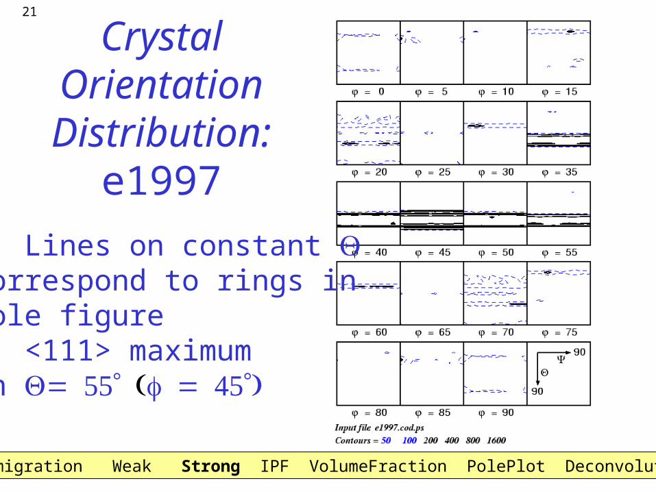
Crystal Orientation

Distribution: e1997

1. Lines on constant correspond to rings inpole figure2. <111> maximumon


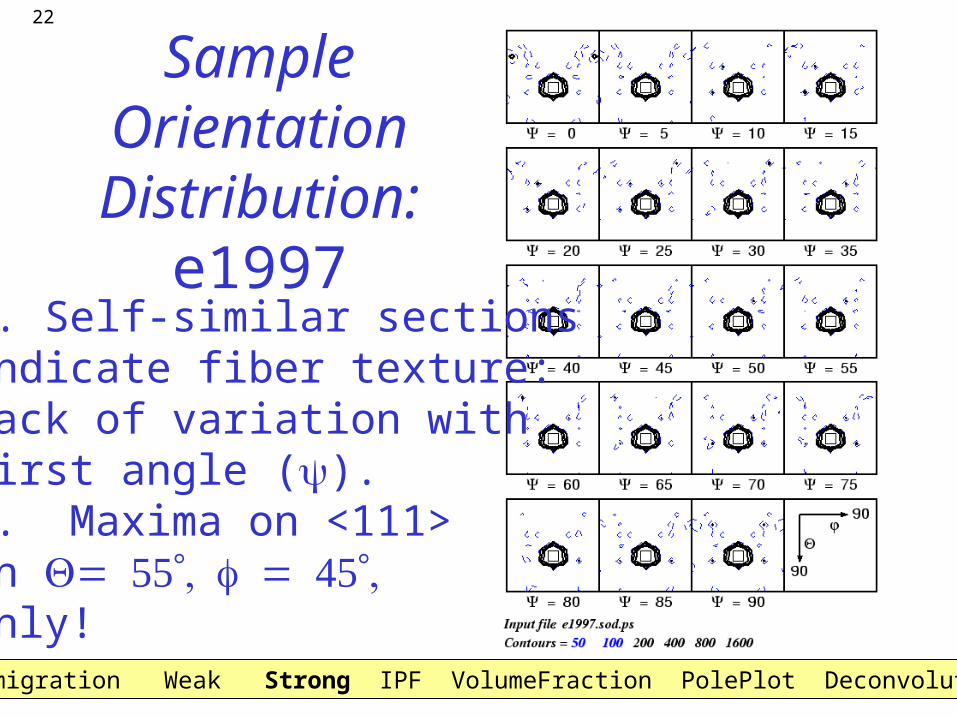
22

Sample Orientation

Distribution: e1997

1. Self-similar sectionsindicate fiber texture:lack of variation withfirst angle ().2. Maxima on <111> on only!


23

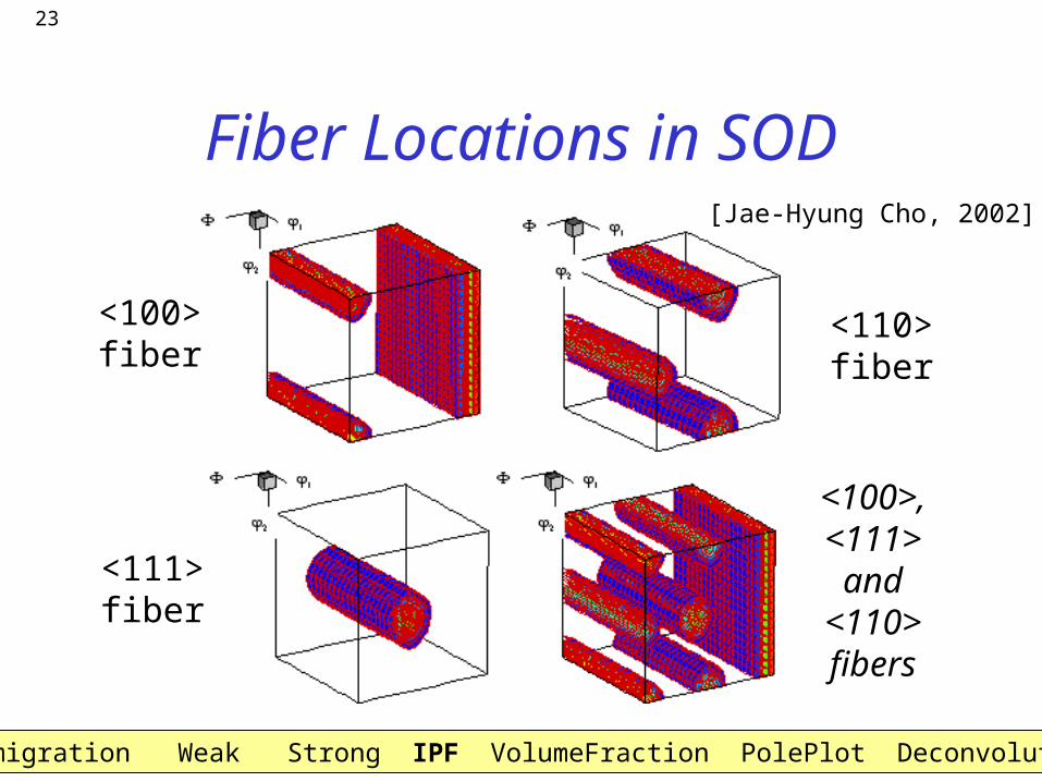
Fiber Locations in SOD

<100>fiber

<111>fiber

<110>fiber

<100>,<111>

and<110>fibers

[Jae-Hyung Cho, 2002]


24

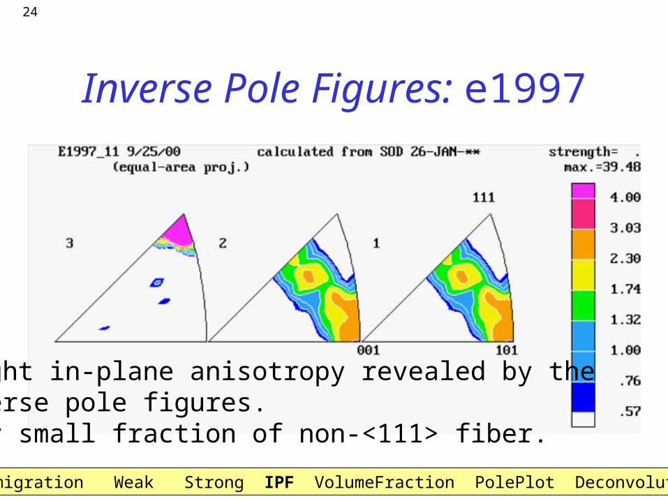
Inverse Pole Figures: e1997

Slight in-plane anisotropy revealed by theinverse pole figures.Very small fraction of non-<111> fiber.


25

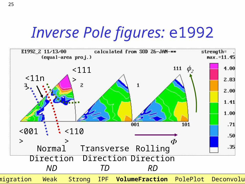
Inverse Pole figures: e1992

<111><11n>

<001> <110>

NormalDirection

ND

TransverseDirection

TD

RollingDirection

RDElectromigration Weak Strong IPF VolumeFraction PolePlot Deconvolution

26

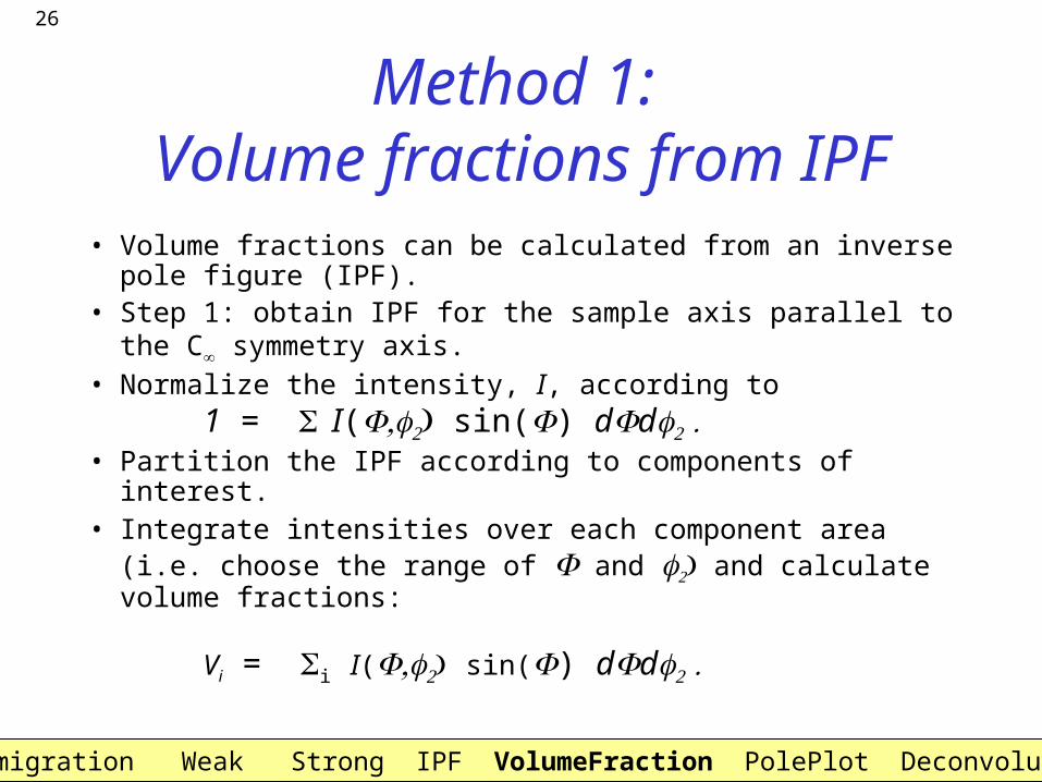
Method 1: Volume fractions from IPF

• Volume fractions can be calculated from an inverse pole figure (IPF).

• Step 1: obtain IPF for the sample axis parallel to the C symmetry axis.

• Normalize the intensity, I, according to 1 = I( sin() dd

• Partition the IPF according to components of interest.• Integrate intensities over each component area (i.e. choose

the range of and and calculate volume fractions:

Vi = i I( sin() dd


27

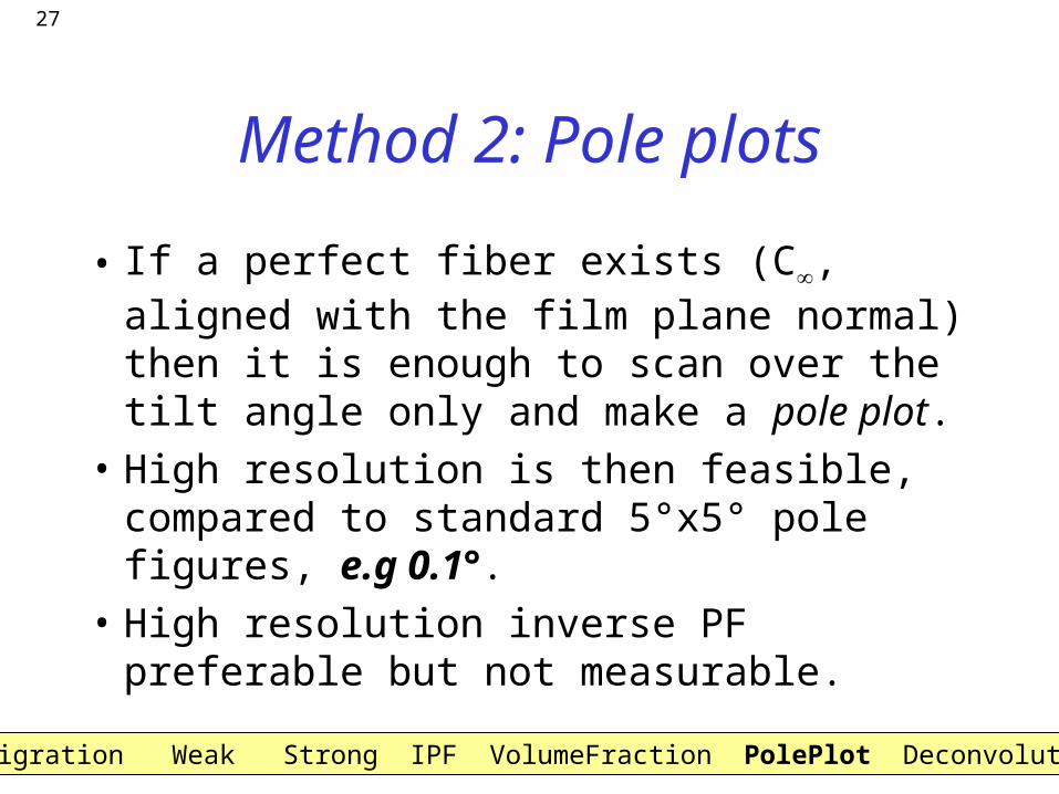
Method 2: Pole plots

• If a perfect fiber exists (C, aligned with the film plane normal) then it is enough to scan over the tilt angle only and make a pole plot.

• High resolution is then feasible, compared to standard 5°x5° pole figures, e.g 0.1°.

• High resolution inverse PF preferable but not measurable.


28

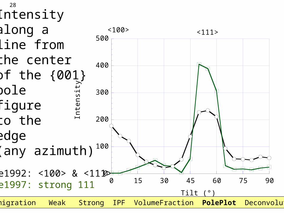
Intensityalong aline fromthe centerof the {001}polefigureto theedge(any azimuth)

e1992: <100> & <111>e1997: strong 111

0

100

200

300

400

500

0 15 30 45 60 75 90

Inte

nsity

Tilt (°)

<100> <111>


29

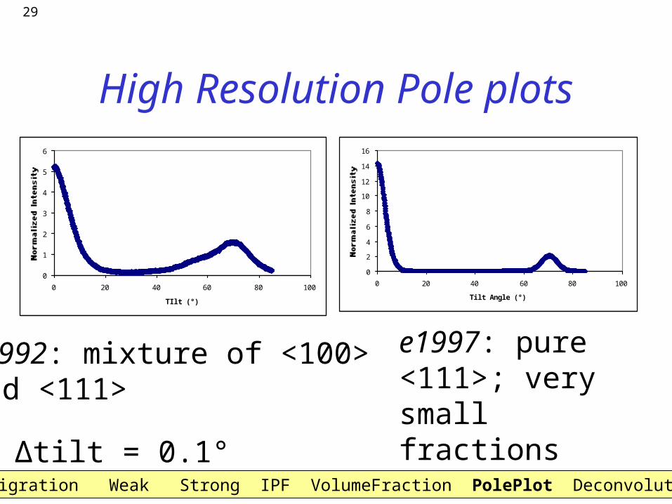
High Resolution Pole plots

0

2

4

6

8

10

12

14

16

0 20 40 60 80 100

Tilt Angle (°)

0

1

2

3

4

5

6

0 20 40 60 80 100

TIlt (°)

e1992: mixture of <100>and <111>

e1997: pure <111>; very small fractions other?∆tilt = 0.1°


30

Volume fractions

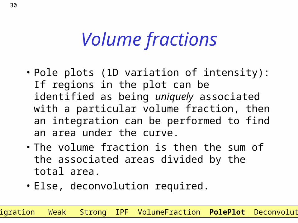
• Pole plots (1D variation of intensity):If regions in the plot can be identified as being uniquely associated with a particular volume fraction, then an integration can be performed to find an area under the curve.

• The volume fraction is then the sum of the associated areas divided by the total area.

• Else, deconvolution required.Electromigration Weak Strong IPF VolumeFraction PolePlot Deconvolution

31

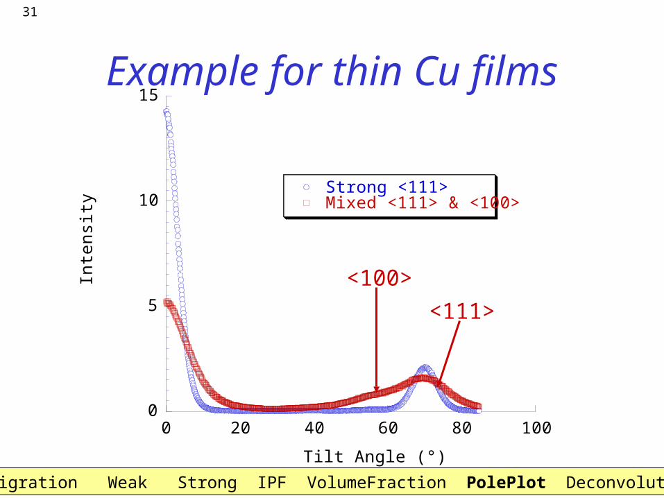
Example for thin Cu films

0

5

10

15

0 20 40 60 80 100

Strong <111>Mixed <111> & <100>

Inte

nsity

Tilt Angle (°)

<100>

<111>


32

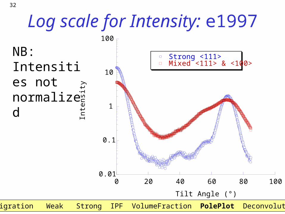
Log scale for Intensity: e1997

0.01

0.1

1

10

100

0 20 40 60 80 100

Strong <111>Mixed <111> & <100>

Inte

nsity

Tilt Angle (°)

NB: Intensities not normalized


33

Area under the Curve

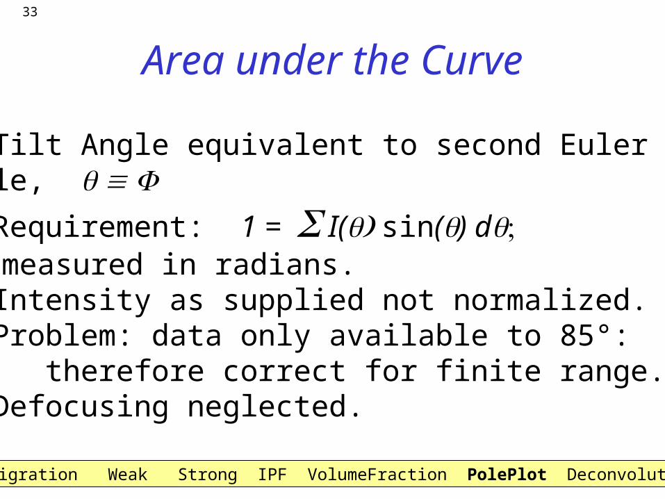
• Tilt Angle equivalent to second Eulerangle,

• Requirement: 1 = I( sin() dmeasured in radians.• Intensity as supplied not normalized.• Problem: data only available to 85°: therefore correct for finite range.• Defocusing neglected.


34

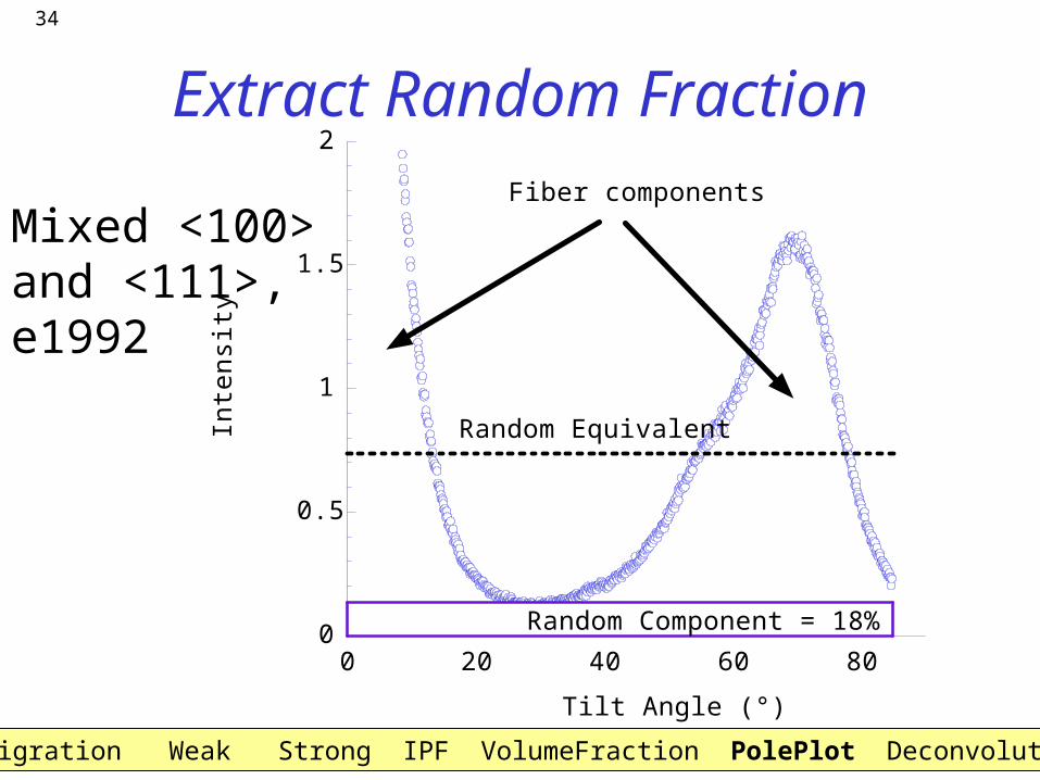
Extract Random Fraction

0

0.5

1

1.5

2

0 20 40 60 80

e1992.111PF.data

Inte

nsity

Tilt Angle (°)

Random Component = 18%

Fiber components

Random Equivalent

Mixed <100>and <111>,e1992


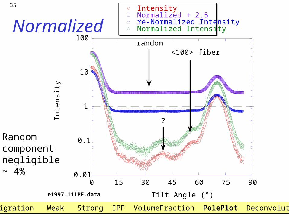
35

Normalized

0.01

0.1

1

10

100

0 15 30 45 60 75 90

e1997.111PF.data

IntensityNormalized + 2.5re-Normalized IntensityNormalized Intensity

Inte

nsity

Tilt Angle (°)

<100> fiberrandom

?

Randomcomponentnegligible~ 4%


36

Deconvolution

• Method is based on identifying each peak in the pole plot, fitting a Gaussian to it, and then checking the sum of the individual components for agreement with the experimental data.

• Areas under each peak are calculated.

• Corrections must be made for multiplicities.


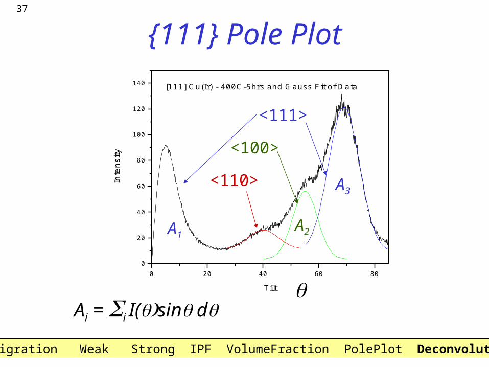
37

0 20 40 60 800

20

40

60

80

100

120

140 [111] Cu(Ir) - 400C-5hrs and Gauss Fit of Data

Inte

nsi

ty

Tilt

<111>

<100>

<110>

{111} Pole Plot

A1A2

A3

Ai = i I(sin d


38

0 10 20 30 40 50 60 70 800

20

40

60

80

100

120

140 Cu(Ir) - 400C-5hrs

Inte

nsi

ty

Tilt

Convolution Raw Data <111>

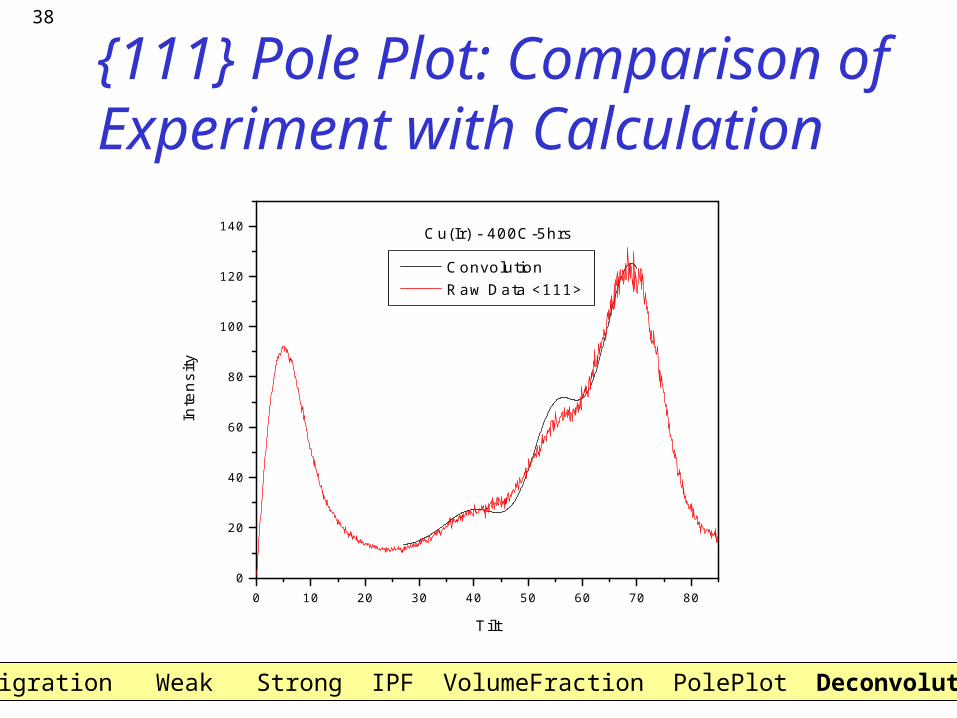
{111} Pole Plot: Comparison of Experiment with Calculation


39

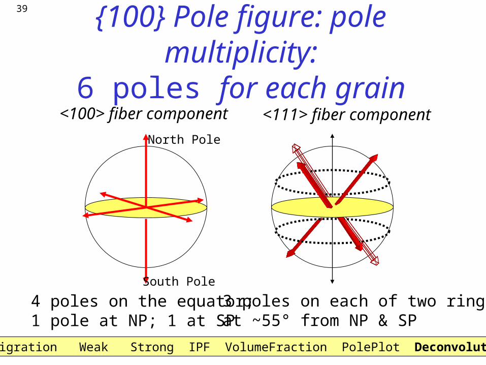
{100} Pole figure: pole multiplicity:6 poles for each grain

<100> fiber component <111> fiber component

4 poles on the equator;1 pole at NP; 1 at SP

3 poles on each of two rings, at ~55° from NP & SP

North Pole

South Pole


40

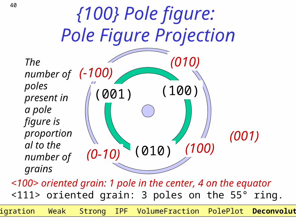
{100} Pole figure: Pole Figure Projection

(100)

(010)

(001)

(001)(100)

(010)(-100)

(0-10)

<100> oriented grain: 1 pole in the center, 4 on the equator<111> oriented grain: 3 poles on the 55° ring.

The number of poles present in a pole figure is proportional to the number of grains


41

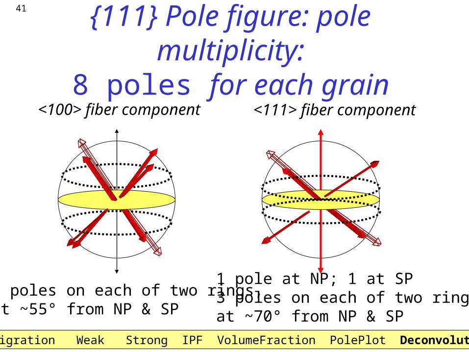
{111} Pole figure: pole multiplicity:8 poles for each grain

<111> fiber component

1 pole at NP; 1 at SP3 poles on each of two rings, at ~70° from NP & SP

4 poles on each of two rings, at ~55° from NP & SP

<100> fiber component


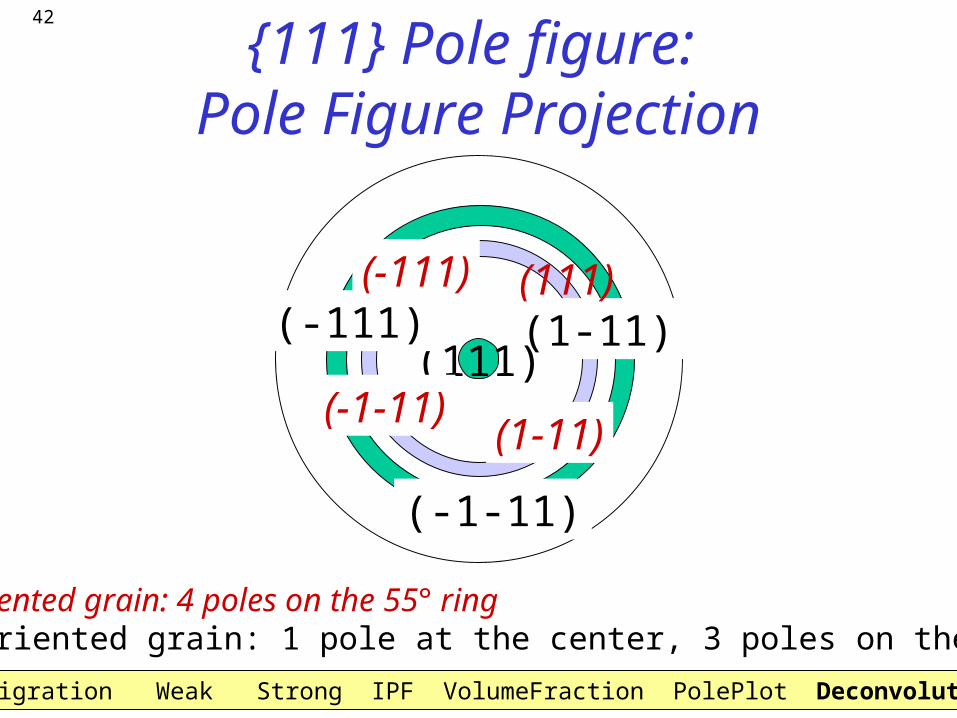
42

{111} Pole figure: Pole Figure Projection

(001)

<100> oriented grain: 4 poles on the 55° ring<111> oriented grain: 1 pole at the center, 3 poles on the 70° ring.

(-1-11)

(1-11)(111)

(1-11)

(111)(-111)

(-1-11)

(-111)


43

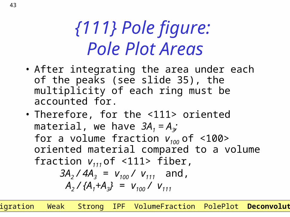
{111} Pole figure: Pole Plot Areas

• After integrating the area under each of the peaks (see slide 35), the multiplicity of each ring must be accounted for.

• Therefore, for the <111> oriented material, we have 3A1 = A3;for a volume fraction v100 of <100> oriented material compared to a volume fraction v111 of <111> fiber,

3A2 / 4A3 = v100 / v111 and, A2 / {A1+A3} = v100 / v111


44

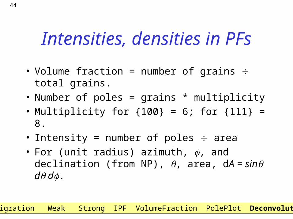
Intensities, densities in PFs

• Volume fraction = number of grains total grains.

• Number of poles = grains * multiplicity• Multiplicity for {100} = 6; for {111} = 8.• Intensity = number of poles area• For (unit radius) azimuth, , and declination (from

NP), , area, dA = sin d d.


45

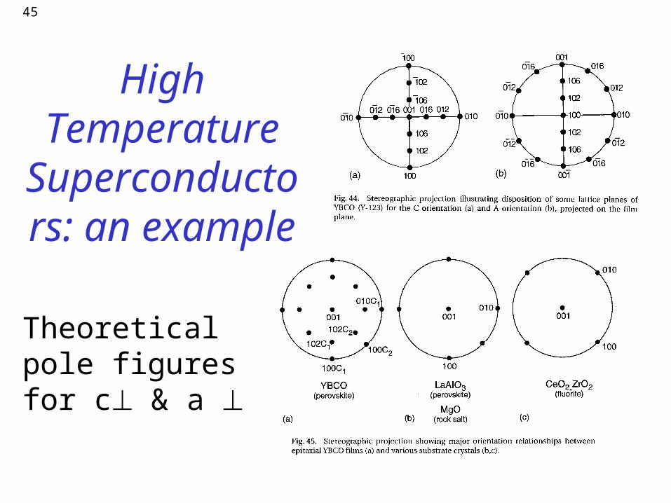
High Temperature

Superconductors: an example

Theoreticalpole figuresfor c & a

46

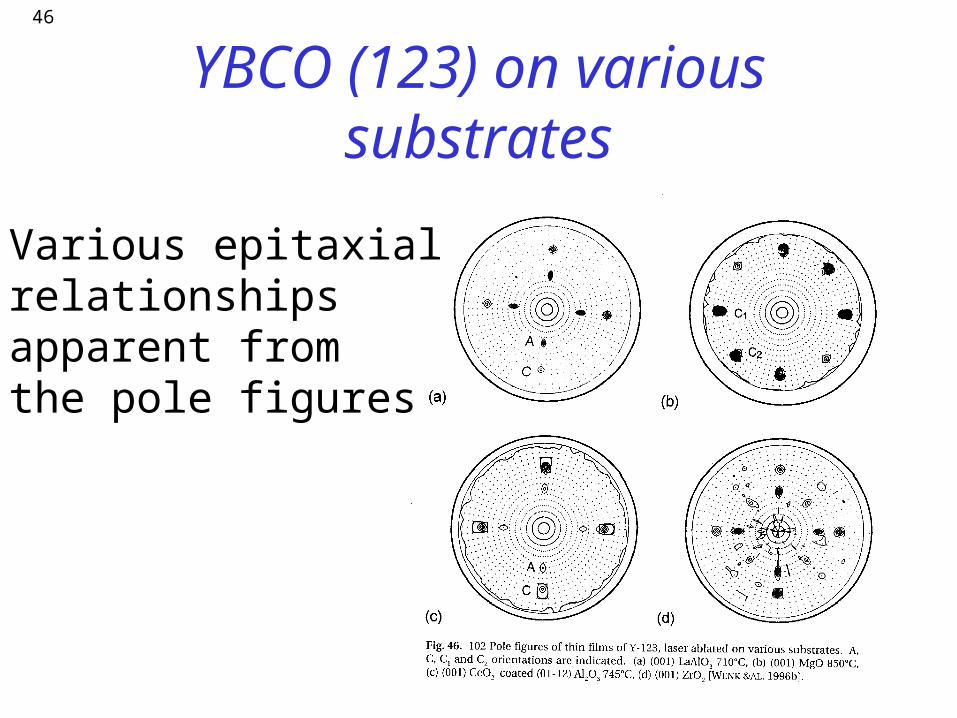
YBCO (123) on various substrates

Various epitaxialrelationshipsapparent fromthe pole figures

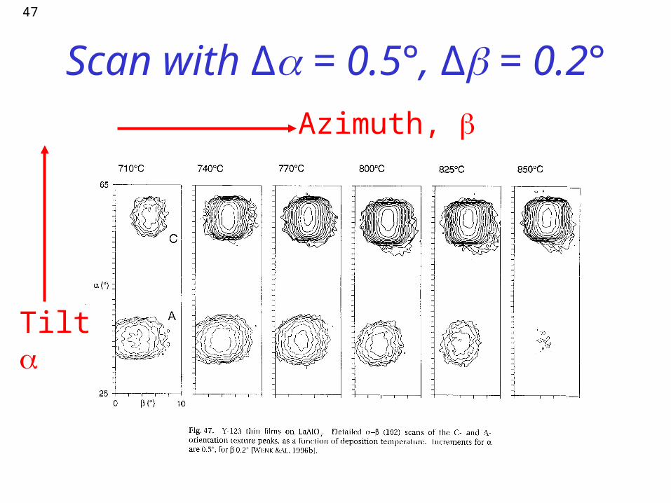
47

Scan with ∆ = 0.5°, ∆ = 0.2°

Tilt

Azimuth,

48

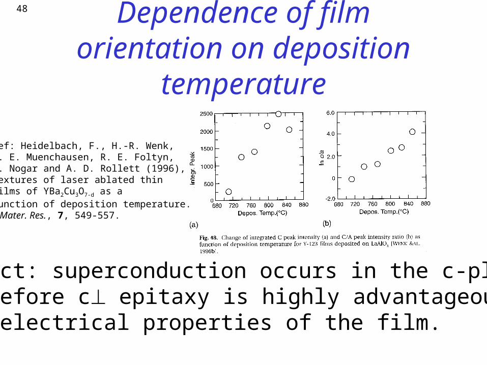
Dependence of film orientation on deposition temperature

Impact: superconduction occurs in the c-plane;therefore c epitaxy is highly advantageous tothe electrical properties of the film.

Ref: Heidelbach, F., H.-R. Wenk, R. E. Muenchausen, R. E. Foltyn, N. Nogar and A. D. Rollett (1996), Textures of laser ablated thin films of YBa2Cu3O7-d as a function of deposition temperature. J. Mater. Res., 7, 549-557.

49

Summary: Fiber Textures• Extraction of volume fractions possible provided that

fiber texture established.• Fractions from IPF simple but resolution limited by

resolution of OD.• Pole plot shows entire texture.• Random fraction can always be extracted.• Specific fiber components may require deconvolution

when the peaks overlap.• Calculation of volume fraction from pole figures/plots

assumes that all corrections have been correctly applied (background subtraction, defocussing, absorption).

50

Summary: other issues

• If epitaxy of any kind occurs between a film and its substrate, the (inevitable) difference in lattice paramter(s) will lead to residual stresses. Differences in thermal expansion will reinforce this.

• Residual stresses broaden diffraction peaks and may distort the unit cell (and lower the crystal symmetry), particularly if a high degree of epitaxy exists.

• Mosaic spread, or dispersion in orientation is always of interest. In epitaxial films, one may often assume a Gaussian distribution about an ideal component and measure the standard deviation or full-width-half-maximum (FWHM).

51

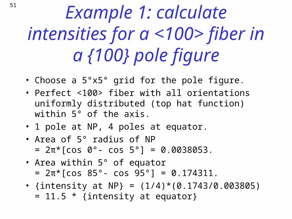
Example 1: calculate intensities for a <100> fiber in a {100} pole

figure• Choose a 5°x5° grid for the pole figure.

• Perfect <100> fiber with all orientations uniformly distributed (top hat function) within 5° of the axis.

• 1 pole at NP, 4 poles at equator.

• Area of 5° radius of NP = 2π*[cos 0°- cos 5°] = 0.0038053.

• Area within 5° of equator = 2π*[cos 85°- cos 95°] = 0.174311.

• {intensity at NP} = (1/4)*(0.1743/0.003805) = 11.5 * {intensity at equator}

52

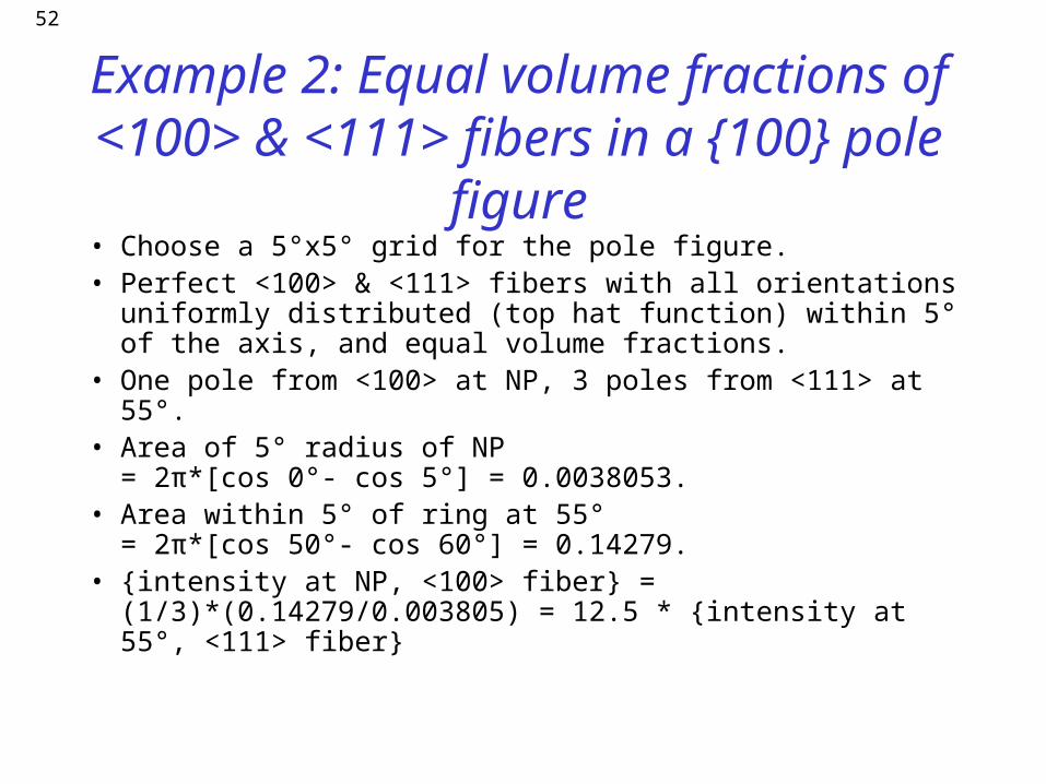
Example 2: Equal volume fractions of <100> & <111> fibers in a {100} pole figure

• Choose a 5°x5° grid for the pole figure.• Perfect <100> & <111> fibers with all orientations

uniformly distributed (top hat function) within 5° of the axis, and equal volume fractions.

• One pole from <100> at NP, 3 poles from <111> at 55°.• Area of 5° radius of NP

= 2π*[cos 0°- cos 5°] = 0.0038053.• Area within 5° of ring at 55°

= 2π*[cos 50°- cos 60°] = 0.14279.• {intensity at NP, <100> fiber} = (1/3)*(0.14279/0.003805)

= 12.5 * {intensity at 55°, <111> fiber}

Documents

1 Fiber Textures: application to thin film textures 27-750, Spring 2007 A. D. (Tony) Rollett, A. Gungor & K. Barmak Acknowledgement: the data for these