Objective trajectories in hybrid classical-quantum dynamics

Jonathan Oppenheim,1 Carlo Sparaciari,1 Barbara Soda,1, 2, 3 and Zachary Weller-Davies1

1Department of Physics and Astronomy, University College London,Gower Street, London WC1E 6BT, United Kingdom

2Dept. of Physics, University of Waterloo, Waterloo, Ontario, Canada3Perimeter Institute for Theoretical Physics, Waterloo, Ontario, Canada

(Dated: November 13, 2020)

Consistent dynamics which couples classical and quantum degrees of freedom exists, providedit is stochastic. This provides a way to study the back-reaction of quantum fields on space-timewhich does not suffer from the pathologies of the semi-classical equations. Here we introduce severaltoy models in which to study hybrid classical-quantum evolution, including a qubit coupled to aparticle in a potential, and a quantum harmonic oscillator coupled to a classical one. We present anunravelling approach to calculate the dynamics. Unlike the purely quantum case, the trajectories(or histories) of this unravelling can be unique, conditioned on the classical degrees of freedom. Thisprovides a potential solution to the “measurement problem” of quantum theory; quantum systemsbecome classical because they interact with a genuinely classical field.

I. INTRODUCTION

We are often interested in the dynamics of composite systems where one system can be considered classical whilethe other must be treated quantum mechanically. In quantum thermodynamics and quantum chemistry, we often havesmall molecules interacting with a large thermal reservoir which can be treated classically. In measurement theorythe quantum system interacts with a macroscopic device which can be considered classical. In gravity, macroscopicobjects such as evaporating black holes radiate thermally, and we imagine there is a regime where we can treat theblack hole space-time classically even though the radiation must still be described by quantum field theory.

There is a lot of debate in the literature on whether one can consistently couple quantum systems and classicalones, and many ways of doing so which although useful in some regimes, are pathological [1–11]. Many proposals forsuch dynamics [12–18] are not completely positive, and since both the density matrix of a quantum system and thephase-space density of a classical system are positive functions or matrices, such maps lead to negative probabilities,and are at best an approximation to the true dynamics. Other proposals, such as semi-classical gravity, are non-linear and thus don’t respect the statistical nature of the density matrix [19, 20]. However, evolution laws introducedin [21] are consistent and have been used to study the collisionless Boltzmann equation [22], discussed in the contextof measurement theory [23], and have been proposed as a fundamental theory coupling quantum fields to classicalspace-time [24, 25]. Because we don’t have a quantum theory of gravity, the prospect of understanding how classicalspace-time and quantum fields interact is exciting, whether the dynamics are fundamental or merely effective. Inaddition to the potential to better understand black hole physics, an effective theory opens up the possibility ofgaining new insights into cosmology, since the quantum nature of vacuum fluctuations are important in structureformation in an expanding universe.

We will not discuss gravity in the present work. Rather the aim here is to introduce basic techniques, and studysome simple systems in order to build up an intuition for how classical systems couple to quantum ones. In particular,we shall see that such coupling not only leads to decoherence of the quantum system [25–27], but also a ”collapse”of the wavefunction, in the sense that the quantum system jumps to a pure state which can be determined from theclassical degrees of freedom. In this sense, we will see that the state of the system can be considered to have someobjectivity, unlike the purely quantum case where a decomposition of the system’s density matrix into pure states (orevolution into a history) is not unique [28, 29]. We also study another feature of hybrid dynamics, namely a trade-offbetween decoherence and diffusion. Quantum systems which have long coherence times necessarily have high diffusionin the classical degrees of freedom. Here, we shall exhibit systems which have this feature. That there is necessarilya trade-off between decoherence of the quantum system and diffusion of the classical one, will be shown in [30].

We shall here consider a qubit and a quantum harmonic oscillator which are coupled to classical degrees of freedomare described by a phase-space manifoldM, and for simplicity in the following we takeM≡ R2n, the space of positionand momentum z = q, p for n particles. The quantum degrees of freedom are described by a Hilbert space H, whichmight be finite or infinite dimensional. Given the Hilbert space, we define the set of positive semi-definite operatorswhose trace is at most unity as S≤1(H). The object describing the state of this composite system at a given time isthe map % :M→ S≤1(H) such that, when the quantum degrees of freedom are traced out, returns a valid probabilitydistribution over the phase-space. We will call this the hybrid-density. Mathematically, we have that the distributionprob(z) = Tr [%(z)] is such that prob(z) ≥ 0 for all z ∈ M, and it is normalized

∫M dz prob(z) = 1. From the above

arX

iv:2

011.

0600

9v1

[qu

ant-

ph]

11

Nov

202

0

2

property it is easy to show that, if the classical degrees of freedom are traced out, the resulting state ρ =∫M dz %(z) is

a valid quantum state (i.e., a positive semi-definite operator with unit trace). The simplest such system is the hybridqubit, whose state can be written as

%(q, p) =

(u0(q, p) c(q, p)c?(q, p) u1(q, p)

)If we integrate over phase space, we obtain the density matrix of the qubit, while if we take the trace of the densitymatrix, we are left with the phase-space density of a classical particle.

A consistent and general form of dynamics for these composite classical-quantum systems is given by a masterequation, first introduced in Ref. [21] and here reported as Eq. (2), which couples the quantum and classical degreesof freedom. This master equation posses several necessary properties; it is linear in the state of the compositeclassical-quantum system, and it is completely positive and trace preserving, so that it’s action preserves the statisticalinterpretation of %(q, p). A valid quantum-classical state is transformed to another valid quantum-classical state, withthe master equation preserving the separation between classical and quantum degrees of freedom. The dynamics isnecessarily stochastic, and it is not generally the case that it arises from the dynamics of a larger quantum system.This makes it attractive as a theory of gravity – for a full discussion of this, along with a discussion on the consistencyof quantum-classical dynamics we refer the reader to [25]. Ref. [25] also introduced a particular form of Eq. (2) whichhas the desired classical limit of Hamiltonian evolution, here presented as Eq. (4).

In this paper, we are interested in understanding the main features of the dynamics generated by this masterequation. In order to study these properties, we generalise a well-known tools from open quantum systems, knownas the unravelling of the master equation [31–33]. In open quantum systems [34, 35], one studies the evolution of aquantum system coupled to an external environment. The most general Markovian evolution of the quantum systemgiven some reasonable assumptions is the GKSL or Lindblad equation [36, 37], whose action over the set of quantumstates forms a semi-group [38]. The dynamics of a quantum state ρ are given by

∂ ρ

∂t= −i [H, ρ] +

∑α,β

λαβLαρL†β −

1

2

∑α,β

λαβ (z)L†βLα, ρ

+

(1)

with H the Hamiltonian of the system, ·, ·+ is the anti-commutator and Lα, Lβ ∈ B(H) are Lindblad operators.Such dynamics arise, for example, when a quantum system is weakly coupled to a very large environment.

The unravelling is a technique that allows us to numerically simulate the evolution of a quantum system generatedby the GKSL equation [31–33, 39–41]. Instead of considering the evolution of the full density matrix describingthe system, in the unravelling one consider a single pure state, which is evolved according to a stochastic dynamics.Multiple paths in the Hilbert space are thus generated by the stochastic dynamics, and by averaging over the paths werecover the evolution of the quantum system. This procedure is computationally advantageous compared to evolvingthe full density matrix, in particular when the dimension of the system is large. Moreover, the unravelling techniqueprovides a different perspective on the evolution of open quantum systems; indeed, the evolution of the system canbe understood as generated by a continuous, deterministic dynamics (when the system does not interact with theenvironment), scattered by discrete jumps of the wave-function (when system and environment interact), which occurstochastically in time [33].

In the quantum case, there is generally not a unique unravelling for the master equation, so one cannot regard aparticular trajectory as actually happening. Indeed, the decomposition of the dynamics in terms of Lindblad operatorsLα and a Hamiltonian H in Eq. (1), is not in general unique. One can rewrite the Lα in terms of some other basis ofoperators. This presents a problem [28, 29] for interpretations of quantum theory which take the trajectories as givinga theory of microscopic state reduction [42], and likewise for the decohering histories approach[43–46]. In contrast, byextending the tools of unravelling to the master equation which generates the dynamics of classical-quantum systems,we shall find that trajectories can be unique conditioned on the classical degrees of freedom (c.f. [47] where theenvironment plays this role). This imbues the unravelled trajectories with an ontological significance and allows oneto interpret the state of the system as ”collapsing” to a particular state. This collapse of the wave-function is heregenerated by the interaction between classical and quantum degrees of freedom rather than the introduction of anad-hoc field as in spontaneous collapse models [48–51]. Classical systems can be in definite states, and we find that aclassical-quantum interaction causes the quantum system to inherit this property. This provides a new resolution ofthe measurement problem of quantum theory – quantum systems become classical because they interact with anothersystem which is itself intrinsically classical (e.g. space-time as in [25]).

However, one needn’t make such an interpretational commitment. The unravelling can merely be considered to bea calculational tool which allows us to better simulate the dynamics of some simple hybrid systems and we presentan algorithm and code for this purpose. We study both the hybrid qubit and hybrid oscillator numerically andanalytically, and explore a relation between the diffusion of the classical degrees of freedom in phase space and the

3

rate of decoherence of the quantum degrees of freedom. Interestingly, this relation provides a way to experimentallytest whether the master equation can be used to construct a ”post-” quantum theory of gravity [25]. We alsostudy the energy of the composite system, defined in terms of the sum of the classical and quantum Hamiltonianoperators. Because this composite energy is not the generator of time-translations, there is no reason to expect it tobe conserved [52] – Noether’s theorem doesn’t apply if the dynamics is not unitary. Nonetheless, insofar as one canhave a classical-quantum Hamiltonian, one might want to keep violations of its conservation small. There are variousmechanisms one can employ for this purpose which we will briefly mention in the discussion. In the gravitationalsetting, the more natural question to consider is whether the constraints are preserved in time, a discussion which wereserve for the future [53].

The paper is structured as follow. In Sec. II we briefly review the hybrid master equation describing the evolution ofclassical-quantum systems, and we extend the unravelling technique to this setting. In Sec. III we study two differenttoy models where the classical degrees of freedom interact with a finite-dimensional quantum system (a qubit). We usethe unravelling technique to simulate the hybrid dynamics, and to identify its main features. In Sec. IV we considerthe case in which the quantum system is infinite-dimensional (a harmonic oscillator), and we repeat our analysis inthis setting, with a special focus on the decoherence of this system. We conclude in Sec. V, and suggest various waysthese models could naturally be extended, for example, by having the quantum dynamics always dependent on phasespace degrees of freedom or by adding in friction terms which would control the diffusion of the classical degrees offreedom in phase space.

II. THE CLASSICAL-QUANTUM MASTER EQUATION AND ITS UNRAVELLING

In this section, we show that the most general master equation governing the dynamics of a classical-quantum(CQ) system can be unravelled, allowing us to efficiently simulate the evolution of different finite-dimensional hybridsystems. Recasting the dynamics under the unravelling formalism provides a useful perspective for understandingthe evolution of CQ systems. Indeed, from this point of view the hybrid system evolves continuously in its classicaland quantum degrees of freedom, and its evolution is interrupted at random times by jumps in both the classicalphase-space and the Hilbert space. It is worth noting that the jumps are here due to the interactions between theclassical and the quantum system, and they are not, as in the case of open quantum systems, due to the presence ofan external environment. Although one can always consider the state of a hybrid classical-quantum system to be therestriction of a pure quantum state on part of an enlarged Hilbert-space, one is not guaranteed that there will be aunitary dynamics on the entire system whose restricted dynamics is of the required form.

Another difference between the unravelling for hybrid dynamics and the one used in open system dynamics concernsthe objectiveness of the jumps. In the case of open quantum systems, a given dynamics can be obtained from anentire family of jumps [35]. There are usually many ways in which one can decompose the dynamics in terms of jumpsin Hilbert space, and so one cannot think of the unravelling as representing actual trajectories that the system makes.In contrast, for some classes of hybrid dynamics, each classical jumps in phase-space is uniquely defined and one canimagine continuously monitoring the classical system through time without disturbing the system. We can thus thinkof the classical trajectories as being ones which objectively occur.

Before we can extend the unravelling technique to case of classical-quantum dynamics, we need to formally introducethe class of hybrid systems we consider, and the form of the master equation describing their evolution. The mostgeneral Markovian CQ dynamics in the case of bounded operators Lα is given by [21–23]

∂ %(z, t)

∂t=− i [H(z), %(z, t)] +

∫d∆

∑α,β

Wαβ (z|z −∆) Lα %(z −∆, t)L†β −1

2

∑α,β

Wαβ (z)L†βLα, %(z, t)

+, (2)

where z = (q1, p1, q2, p2, . . .) ∈ R2n is the vector of phase space coordinates for n systems, and %(z, t) is a classical-quantum state at time t. The Hamiltonian H(z), which appears in the commutator with the CQ state, controls theunitary evolution of the quantum system, and in principle depends on the classical degrees of freedom. For each αand β, the rate Wαβ (z|z −∆) governs the transition of the classical degrees of freedom from z −∆ to z, as well as

the jump of the quantum state due to the map Lα ·L†β . For the master equation to preserve the norm of the quantum

state (once the classical degrees of freedom have been traced out), we need to require that

Wαβ (z) =

∫d∆Wαβ (z + ∆|z) ∀α, β. (3)

The hybrid master equation (2) is completely positive (CP) over the classical and quantum degrees of freedom, andtrace-preserving (TP) in the sense that the normalisation condition

∫dzTr [%(z)] = 1 is preserved. Furthermore, its

4

structure is such that the separation between classical and quantum degrees of freedom is preserved i.e. %(z) is alwaysa subnormalised density matrix. Finally, the master equation is clearly linear in the CQ state. All these propertiesensure that a CQ state is mapped into another CQ state by the dynamics generated by Eq. (2).

Although Eq. (2) gives the general form of the dynamics, we are interested in evolution which in some limitreproduces classical Hamiltonin dynamics. This was done in [25] by expanding Wαβ in terms of moments of δ anddemanding that the 1st moment reduce to the Poisson bracket of the state with some Hamiltonian. The particularform we will explore here, is given by taking matrix Wαβ (z|z −∆) such that∫

d∆∑α

Wαβ (z|z −∆) Lα %(z −∆, t)L†β =∑αβ

1

ταβeταβ hαβ(z), · Lα %(z, t)L†β , (4)

where ταβ > 0 can be understood as a rate, ·, · is the Poisson bracket, and the functions hα(z) are associated withthe CQ interaction Hamiltonian

H(z) =∑

hαβ(z)L†βLα (5)

The resulting master equation is

∂ %(z, t)

∂t= −i [H(z), %(z, t)] +

∑αβ

1

ταβ

(eταβ h

α(z), · Lα %(z, t)L†β −1

2

L†βLα, %(z, t)

+

). (6)

and we see that to 0’th order in the ταβ , this master equation reproduces Hamiltonian dynamics in the appropriatelimit. Namely, if we expand the exponential in the right hand side of the equation for small values of the parametersταβ ’s, we obtain

∂ %(z, t)

∂t=− i [H(z), %(z, t)] +

∑α

1

ταβ

(Lα %(z, t)L†β −

1

2

L†βLα, %(z, t)

+

)+∑hαβ(z), Lα%(z)L†β+ · · · (7)

where the parameters ταβ ’s play the role of the relaxation rates The first term of Eq. (7) is the dynamics of thequantum system, which can in principle depend on the classical degrees of freedom. In this way, it represents theevolution of the quantum system as controlled by the classical one. The next two terms are purely Lindbladiandynamics, and in the limit that ταβ → 0, it can lead to rapid decoherence of the quantum system. The final term isthe interaction Hamiltonian dynamics we desire, namely under the trace, it is Tr [H, %]. We can think of it as thecounter-part to the commutator in the sense that it gives the back-action of the quantum system on the classical one,while the commutator reflects the influence of the classical system on the quantum one. Indeed, in the classical limit,we expect −i[H(z), %] to act as the Poisson bracket with respect to the degrees of freedom of the quantum system,

while in this limit one can verify that hαβ , Lα%L†β are the additional terms of the Poisson bracket with respect to thedegrees of freedom of the classical system. We can take purely classical dynamics to correspond to identity Lindbladoperators which we take to be Lα=0 = I. If we wish this classical dynamics to be purely deterministic, then we cantake τ00 → 0, so that we have a term in the dynamics given by HC , % with the classical Hamiltonian is defined as

HC(z) := h00(z) I. (8)

Higher order terms can lead to diffusion in phase space. For example, at first order in τ , Eq. (7) will acquire termsof the form

D(%) = τDαβp,ij(z)Lα

∂2%

∂pi∂pjL†β + τDαβ

qp,ij(z)Lα∂2%

∂qi∂pjL†β + τDαβ

q,ij(z)Lα∂2%

∂qi∂qjL†β (9)

where for ease of presentation we have taken all ταβ = τ . Such terms lead to diffusion in phase-space, with Dαβp,ij(z)

being the diffusion term usually found in the Fokker-Planck equation, or arising from Langevin dynamics. WhenWαβ(z|z − ∆) is deterministic in q, but diffusive in p, we shall refer to it as dynamics of the Langevin type. It ispossible to also have terms appearing in the expansion which give rise to friction. We discuss such master equationsin greater detail in Sec. V. If the dynamics is of the Langevin type, then one can verify that the equation of motionfor q is unchanged by the diffusive terms appearing in Eq. (7). Inverting this expression gives p(q, q). On the other

hand, master equations which contain terms Dαβqp,ij and Dαβ

q,ij(z) in their expansion, we shall call q-diffusive and we

will discuss such master equations in more detail elsewhere. Care should be taken in any expansion of Wαβ(z|z −∆)– although the full dynamics is completely positive, if we truncate our expansion to any finite order, it is not.

5

A. Unravelling of the CQ dynamics

In the quantum open system formalism, the unravelling of a master equation takes the master equation governingthe evolution of the density matrix, and divides it up into trajectories – i.e. probabilities assigned to an ensemble ofhistories, where each history is the evolution of a pure quantum states which either undergoes a continuous evolutionor jumps from the one state to another as a result of a Lindblad operator being applied to it. Due to the stochasticnature of the unravelling, the initial state is mapped into different final states by the same evolution. If we record eachevolution in time (or trajectory) and we average over them, we re-obtain the evolution law for the density matrix,as given via the master equation (in the limit of infinite trajectories and infinitesimal time steps). The unravellingof the CQ master equation proceeds in analogy with the quantum one, and in this section we provide an algorithmto unravel the dynamics given by Eq. (2), where in addition we consider a fully classical term, given by the Poissonbracket between a classical Hamiltonian HC(z) and the hybrid state,

∂ %(z, t)

∂t=− i [H(z), %(z, t)] + HC(z), %(z, t)

+

∫d∆

∑α,β

Wαβ (z|z −∆) Lα %(z −∆, t)L†β −1

2

∑α,β

Wαβ (z)L†βLα, %(z, t)

+.

Specifically, we will provide the tools to generate different classical-quantum trajectories, and we will show that theaverage of these trajectories coincides with the evolution of the CQ state under the above master equation.

In the following, we consider the case in which the matrix of rates Wαβ (z|z −∆) are diagonal in α, β. If this matrixis not diagonal in the same basis at each point, we can introduce unitary operators u(z) that diagonalize it,

W ′γ (z|z −∆) = uγ,α(z)Wαβ (z|z −∆) u†β,γ(z), (10)

and use the new Lindblad operators in the unravelling procedure, L′γ(z) = uγ,α(z)Lβ . In this way, the same Lindbladoperator acts on the left and the right of the CQ state in Eq. (2), and we can use the same procedure explained in thefollowing, with the difference that now the Lindblad operators additionally depends on the phase space coordinate z.The central object of this study is a pure CQ state, that is,

|%(z, t)〉 = δ(z − z(t)) |φ(t)〉 , (11)

where |φ(t)〉 is a quantum state independent of the classical degrees of freedom. This object represent a classical-quantum system, centred in the point z(t) of the phase space, and described by the quantum state |φ(t)〉.

The first step in the unravelling procedure is the discretisation of the dynamics of the CQ state; we fix a timeinterval δt, and the evolution of the CQ state is given for multiples of this interval. It is worth noting that theunravelling evolution is exact at first order in this parameter, and coincides with the one given by the master equationin the limit of δt→ 0. We now outline the procedure for generating each trajectory, and we will then show that whenwe average over trajectories, we obtain the CQ master equation. For a given point z in phase space, at each timestep we either update the state with a continuous evolution, or with a jump in the classical and quantum degrees offreedom. When the evolution is continuous, we apply to the quantum part of the CQ state a unitary evolution givenby the (non-Hermitian) effective Hamiltonian

Heff(z) = H(z)− i

2

∑α

Wα (z)L†αLα, (12)

which is composed by the Hamiltonian H(z), which appears in the commutator of Eq. (2), and by the operatorappearing in the anti-commutator of the same equation. The classical part of the CQ state is instead subjected to atranslation in phase space generated by the classical Hamiltonian HC(z), which appears in the Poisson bracket in themaster equation. In order to evolve the CQ state with a jump, we first need to choose at random a value of the tuple(α,∆) from the (un-normalised) distribution Wα (z|z −∆). The α parameter specifies which Lindblad operator Lαis performed over the quantum state, while the ∆ parameter quantifies the shift performed over the classical degreesof freedom.

The unravelling algorithm is then defined by the following set of instructions, that specify how to update a pureCQ state at time t under continuous or jumping evolution,

|%(z, t+ δt)〉 =

1√

N0(z,t)(I− i δtHeff(z)) |%(z − δtΩ∇HC(z), t)〉 with p0(z, t),

1√Nα,∆(z,t)

Lα |%(z −∆, t)〉 with pα,∆(z, t).(13)

6

At each time step, the hybrid pure state can be updated either continuously, first line in the right hand side of theabove equation, or with a jump, second line. The type of evolution is chosen at random; the probability of updatingthe state with a continuous evolution is given by p0(z, t), while the probability of evolving it with a jump is givenby pα,∆(z, t), where α specifies the quantum jump and ∆ specifies the classical one. In the continuous evolution, the

quantum degrees of freedom are evolved by the unitary operator U(z) = e−iδtHeff(z), that we have expanded at firstorder in δt, while the continuous shift in the classical degrees of freedom is generated by the operator eδt HC(z),·.

The gradient vector ∇HC(z) = (∂q1HC(z), ∂p1HC(z), . . .)

T ∈ R2n, while

Ω =

n⊕k=1

(0 1−1 0

)∈M2n,2n(R), (14)

is the symplectic matrix. By iterating the procedure in Eq. (13),we can produce a single trajectory. Different iterationsprovide different trajectories, since at every time step the CQ state is evolved either continuously or with a jump.

The pure CQ states produced by the unravelling technique are normalized. In the following, we provide thenormalization coefficient for both the continuous and jumping evolution, and the probability that either evolutionoccurs. For simplicity, in the rest of the section we suppress the time t dependence. The notmalization coefficient aregiven as

N0(z) = δ(z − z)(

1− δt∑α

Wα (z) 〈φ|L†αLα |φ〉), (15a)

Nα,∆(z) = δ(z − (z + ∆)) 〈φ|L†αLα |φ〉 , ∀α,∆, (15b)

where we have used the form of the CQ pure state, given in Eq. (11), and we are only considering terms in thefirst order of the time step δt. In the next section we explicitly derive these coefficients. At a given time step, theprobability of evolving the pure CQ state continuously or with a jump is given by,

p0(z) = N0(z), (16a)

pα,∆(z) = δtWα (z|z −∆) Nα,∆(z), ∀α,∆. (16b)

It is easy to see that the above distribution is a valid probability distribution over the phase space. Clearly, eachprobability distribution is non-negative, and the distribution is normalised,∫

dz

(p0(z) +

∑α

∫d∆ pα,∆(z)

)= 1− δt

∑α

(∫dzWα (z) δ(z − z)

)〈φ|L†αLα |φ〉

+ δt∑α

∫d∆

(∫dzWα (z|z −∆) δ(z − (z + ∆))

)〈φ|L†αLα |φ〉

= 1− δt∑α

(Wα (z)−

∫d∆Wα (z + ∆|z)

)〈φ|L†αLα |φ〉 = 1, (17)

where the last equality follows from Eq. (3).Before concluding the section, let us comment on an interesting feature of the unravelling of the hybrid master

equation, which is not shared by its quantum counterpart. If a unique shift ∆ in the classical degrees of freedom isassociated with each Lindblad operator Lα, then by monitoring the classical degrees of freedom we have completeknowledge on the jumps that occur in the quantum part of the hybrid state. Furthermore, the quantum evolutionconditioned on the classical degrees of freedom is unique, since only a specific sequence of jumps could produce thesequence of shifts in the classical part. The hybrid state can be said to actually make the transitions given in Eq. (13).This is in contrast with the unravelling for open quantum systems, where the lack of a classical system which can bemonitored makes it impossible to single out different trajectories in the Hilbert space.

B. From unravelling to the CQ master equation

We can now show that the update rule presented in Eq. (13) reproduces, at first order in δt, the same dynamics ofthe hybrid master equation. First, let us derive the normalization coefficients shown in Eqs. (15). To compute thenormalization of the continuously evolved state, we need to Taylor expand it and truncate the expansion at first orderin δt. It is straightforward to show that

|%(z − δtΩ∇HC(z))〉 = (1 + δt HC(z), · ) |%(z)〉+O(δt2). (18)

7

The normalization coefficient is then given by

N0(z, t) = 〈%(z − δtΩ∇HC(z), t)|(I + i δtHeff(z)†

)(I− i δtHeff(z)) |%(z − δtΩ∇HC(z), t)〉

= 1 + δt HC(z), 〈%(z, t)|%(z, t)〉 − δt∑α

Wα(z) 〈%(z, t)|L†αLα |%(z, t)〉+O(δt2)

= 1− δt∑α

Wα (z) 〈%(z, t)|L†αLα |%(z, t)〉+O(δt2),

where the second line follows from the Taylor expansion in Eq. (18), from the form of the effective Hamiltonian Heff(z)and from Leibniz’s rule of the Poisson bracket, while the last line follows from the fact that |%(z, t)〉 is normalized.The normalization of the CQ pure state after a jump is simply

Nα,∆(z) = 〈%(z −∆, t)|L†αLα |%(z −∆, t)〉 . (19)

We can now derive the master equation (2) (equipped with the additional fully-classical term) from the update rulegiven in Eq. (13). To so so, we express the state |%(z, t+ δt)〉 as a density operator, and we re-write it as a mixtureover the possible evolutions the system undergoes. Let us first consider the continuous update for the CQ densityoperator, which we refer to as ρ0(z, t+ δt), where we truncate at first order in δt,

ρ0(z, t+ δt) =1

N0(z, t)

(|%(z, t)〉 〈%(z, t)|+ δt HC(z), |%(z, t)〉 〈%(z, t)|

− i δt [H(z), |%(z, t)〉 〈%(z, t)|]− δt

2

∑α

Wα (z)L†αLα, |%(z, t)〉 〈%(z, t)|

+

),

where we have used the definition of Heff(z), see Eq. (12), and [·, ·] is the commutator while ·, ·+ is the anti-commutator. When the evolution is given by an α-jump in the quantum degrees of freedom, and by a ∆-jump in theclassical ones, we find the following density operator

ρα,∆(z, t+ δt) =1

Nα,∆(z, t)Lα |%(z −∆, t)〉 〈%(z −∆, t)|L†α. (20)

We can now express the overall evolution of the state by weighting the different updates with the correct probabil-ities, given in Eq. (16). Thus, we find that

|%(z, t+ δt)〉 〈%(z, t+ δt)| = p0(z, t) ρ0(z, t+ δt) +∑α

∫d∆ pα,∆(z, t) ρα,∆(z, t+ δt)

= |%(z, t)〉 〈%(z, t)|+ δt HC(z), |%(z, t)〉 〈%(z, t)|

− i δt [H(z), |%(z, t)〉 〈%(z, t)|]− δt

2

∑α

Wα (z)L†αLα, |%(z, t)〉 〈%(z, t)|

+

+ δt∑α

∫d∆Wα (z|z −∆)Lα |%(z −∆, t)〉 〈%(z −∆, t)|L†α, (21)

and if we rearrange the above equation by moving |%(z, t)〉 〈%(z, t)| from the right to the left hand side, we divide byδt, and we send δt→ 0, we obtain

∂

∂t|%(z, t)〉 〈%(z, t)| =− i [H(z), |%(z, t)〉 〈%(z, t)|] + HC(z), |%(z, t)〉 〈%(z, t)|

+

∫d∆

∑α

Wα (z|z −∆)Lα |%(z −∆, t)〉 〈%(z −∆, t)|L†α

− 1

2

∑α

Wα (z)L†αLα, |%(z, t)〉 〈%(z, t)|

+. (22)

As a last step, we need to move from a CQ pure state |%(z, t)〉 to a (possibly mixed) CQ state %(z, t). To do so, weperform an average over the classical-quantum configurations of the initial state, that is, we average over a phasespace distribution Pps of initial points z(t = 0) = z0, as well as a distribution Pq over the initial quantum states|φ(t = 0)〉 = |φ0〉. Thus, by applying this average over the CQ pure state |%(z, t)〉, we obtain

%(z, t) = E[|%(z, t)〉 〈%(z, t)|] =

∫dz0 dφ0 Pps(z0)Pq(φ0) |%(z, t)〉 〈%(z, t)| . (23)

If we now perform the average in Eq. (22), we obtain the CQ master equation.

8

III. MAIN FEATURES OF HYBRID DYNAMICS IN QUBIT TOY MODELS

In this section we present a few toy models to illustrate the main features of the hybrid dynamics generated bythe master equation (2). The simplest hybrid dynamics we can consider is that of a spin half particle in a classicalpotential, which in our examples is taken to be linear. For each of the toy models we derive, both analyticallyand numerically, the dynamics of the corresponding hybrid system. To numerically evolve the CQ state we use theunravelling procedure presented in the previous section. We tailor the unravelling to the specific master equation usedfor the toy models, see Eq. (25). This unravelling procedure is shown in Appendix B.

The main features of the hybrid dynamics, that are highlighted in our toy models, are i) the presence of stochasticcollapses of the quantum degrees of freedom, ii) a trade-off between the classical diffusion in phase space and thequantum decoherence, and iii) the fact that energy is not conserved by the dynamics. More specifically, we find thatthe interaction between classical and quantum degrees of freedom generates a sudden collapse in the latter. Thiscollapse occurs when the CQ state is subjected to a jump, that is, when the classical degrees of freedom are shiftedin phase space and a Lindblad operator acts over the quantum state. If the Lindblad operators are associated withunique shifts in the classical degrees of freedom, we find that the quantum dynamics can be unambiguously recordedby monitoring the classical one, see for example Fig. 1. Furthermore, we find that the rate of dechoerence of thequantum degrees of freedom is linked to the rate of diffusion of the classical ones; the faster the quantum statedecoheres, the slower the classical degrees of freedom spread in phase space. This is not a specific feature of the toymodels we study, but rather a general property of the hybrid dynamics, as shown in Ref. [30]. Finally, we find thatthe average energy of the toy models studied is not conserved by the hybrid dynamics. This should not come as asurprise, since the Hamiltonian operator appearing in Eq. (2) is not the generator of the dynamics. A detailed studyof the conservation laws and symmetries present in the hybrid dynamics is performed in Ref. [53].

Let us introduce the toy models we study in this section, namely, a single spin half particle in a classical potential.The position and momentum of the particle are taken to be the classical degrees of freedom z = (q, p), while the spinof the particle (s = 1

2 ) is the quantum one. To simplify the notation, we take the transition matrix in the hybridmaster equation (6) to be diagonal in α, β (if the transition matrix is not diagonal, we have shown in the previoussection that we can always diagonalise it).

For a spin- 12 particle, the most general quantum Hamiltonian can be written as λ · σ where λ is a vector in R4

and σ = I, σx, σy, σz is the vector of Pauli matrices. By having this depend on the classical degrees of freedom, wecause the classical and quantum system to interact. Let us take the interaction term of the CQ-Hamiltonian to be

HI(q, p) = B(q) (ω0 |0〉 〈0|+ ω1 |1〉 〈1|) , (24)

where the coupling constant B(q) depends on the position of the particle q, and the operator is diagonal in the basis|0〉 , |1〉. By comparing the above interaction Hamiltonian with the general form of Eq. (5), we can easily see thatwe are left some freedom in the choice of the Lindblad operators Lαα 6=0 and of the functions hα(z). By exploitingthis freedom, we will study two different CQ models describing a particle in a linear potential. In both cases, we

choose a classical Hamiltonian HC(q, p) = p2

2m , that is, the one for a free particle of mass m. One could imagine apurely quantum evolution determined by a Hamiltonian which is not dependent on classical degrees of freedom, butin analogy with the gravitational case we will not consider it here. Finally, we demand the rates τα 6=0’s to be all equalto τ > 0, so that no non-trivial Lindblad operator acts more often than the others.

The CQ master equation (6) for the case we are considering is then given by

∂ %(z, t)

∂t= −i [HI(z), %(z, t)] +

1

τ0

(eτ0 HC(z), · − 1

)%(z, t)

+1

τ

∑α6=0

(eτ h

α(z), · Lα %(z, t)L†α −1

2

L†αLα, %(z, t)

+

). (25)

The first term on the right is the evolution of the quantum degrees of freedom and it depends on the position of theclassical particle. The The next term is the purely classical evolution. If we take the rate τ0 to be a finite positivevalue, this classical evolution is stochastic, while if it tends to 0 it is determinstic. In the former case, we will see thatthe equation can be solved analytically. When τ0 → 0, the purely classical evolution is given by the Poisson bracketsbetween the classical Hamiltonian and the CQ state, HC(z), %(z, t) . In this second case, we analyse numericallythe dynamics generated by the master equation, using the unravelling method shown in App. II A. The final set ofterms, gives the backreaction of the qubit on the classical degrees of freedom.

9

A. Qubit evolution with diagonal Lindblad operators in a linear potential

The first toy model we consider is a spin half particle interacting with a linear potential through Lindblad operatorsthat are diagonal in the interaction Hamiltonian eigenbasis |0〉 , |1〉. We make the following choice for the operators,

Lα=1 = |0〉 〈0| , (26a)

Lα=2 = |1〉 〈1| . (26b)

Once the Lindblad operators are defined, they fix uniquely the functions hα(q, p). Indeed, in order to identify theinteraction Hamiltonian HI(q, p) in Eq. (24) with the expression in Eq. (5), we need to define these functions as

hα=1(q, p) = ω0B(q), (27a)

hα=2(q, p) = ω1B(q). (27b)

It is worth noting that, for a given interaction Hamiltonian, the above choice of Lindblad operators and hα(q, p)functions is not unique. In the next section, for instance, we consider non-diagonal operators that nonetheless returnthe same interaction Hamiltonian, but generate a completely different dynamics. Furthermore, one could chose thesame Lindblad operators as we did above, but with a different normalization. To re-obtain the correct HamiltonianHI(q, p) we then need to scale the functions hα(q, p) consistently. Notice that the normalization of the Lindbladoperators influences the rate at which the operator is applied, while the function hα(q, p) regulates the amplitude ofthe shifts in the classical degrees of freedom. This freedom in the Lindblad operators and the functions hα(q, p) islinked to the fact that the interaction Hamiltonian is not the generator of the hybrid dynamics of Eq. (2), and this ishighlighted by the fact that this operator is in fact not conserved by the evolution.

In this example, we consider a potential linearly dependent in position, so that B(q) = qB, where B has a constantvalue. We can express the CQ state %(q, p, t) as

%(q, p, t) =

(u0(q, p, t) c(q, p, t)c?(q, p, t) u1(q, p, t)

), (28)

where ui(q, p, t) is the population of the quantum state |i〉 (for i = 0, 1), and c(q, p, t) is the coherence.We now re-write the CQ master equation given in Eq. (25), in terms of the populations and the coherence of the

state %(q, p, t). In the equations below, we take τ0 → 0, so as to obtain a system of non-local differential equations.When we solve the equations analytically, however, we will require τ0 to be a positive (albeit small) constant. Thedynamics of the populations and coherence is thus given by

∂ ui(q, p, t)

∂t= − p

m

∂ ui(q, p, t)

∂q+

1

τ

(ui(q, p+ ωiBτ, t)− ui(q, p, t)

), i ∈ 0, 1 , (29a)

∂ c(q, p, t)

∂t= −iqB (ω0 − ω1) c(q, p, t)− p

m

∂ c(q, p, t)

∂q− 1

τc(q, p, t). (29b)

It is worth noting that the equation for the coherence can be solve analytically, and the solution has the form

c(q, p, t) = c(q − p

mt) e−iqB(ω0−ω1)t− t

τ , (30)

for any function c(q − pm t) in C1, the set of all continuously differentiable functions. We thus see that the coherence

term decays exponentially fast. We will see that this is a result of the quantum system collapsing to the 0 or 1 statewhile making a momentum jump.

1. Analytical and numerical evolution of populations

In order to study the evolution of the populations analytically, we can re-express Eq. (29a) as a stochastic equation,see App. A. To do so, we do not send to 0 the rate τ0 in Eq. (25), and we obtain the following evolution for thepopulations,

∂ ui(q, p, t)

∂t=

1

τ0

(ui(q −

p

mτ0, p, t)− ui(q, p, t)

)+

1

τ

(ui(q, p+ ωiBτ, t)− ui(q, p, t)

), i ∈ 0, 1 , (31)

10

−0.009 −0.003 0.003 0.009q (m)

−0.2

−0.1

0.0

0.1

0.2p

(kg·m·s−

1)

u0u1

Time t = 0.02 s

0.00000.02000.04000.06000.08000.10000.12000.1400

−0.009 −0.003 0.003 0.009q (m)

−0.2

−0.1

0.0

0.1

0.2

p(k

g·m·s−

1)

u0

u1

Time t = 0.06 s

0.00000.00150.00300.00450.00600.00750.00900.0105

−0.009 −0.003 0.003 0.009q (m)

−0.2

−0.1

0.0

0.1

0.2

p(k

g·m·s−

1)

u0

u1

Time t = 0.10 s

0.00000.00060.00120.00180.00240.00300.00360.0042

FIG. 1. The evolution of the population u0(q, p, t) and u1(q, p, t) in phase space, under the CQ qubit dynamics with diagonalLindblad operators. The initial CQ state is δ(q)δ(p) |+〉, where |+〉 = 1√

2(|0〉+ |1〉). The interaction with the field makes

the quantum state stochastically collapse into either |0〉 or |1〉 at a rate given by ωτ

. The same collapse shifts the classicalmomentum of the particle by ±Bτ , depending on the quantum state it projects onto. By monitoring the classical degrees offreedom, we can establish the state of the quantum system. Indeed, a particle in the state |0〉 has negative momentum, whereasa particle in |1〉 has positive momentum. The evolution of the populations is shown for t = 0.02 s, 0.06 s and 0.1 s. The state isevolved for t = 0.1 s, with time steps of δt = 10−4 s, and the jump rate is τ = 10−2 s. The constant B = 1 J · s ·m−1, the massm = 1 kg, and the frequencies are ω0 = −ω1 = ω = 1 s−1.

The solution of this equation is given in the appendix for general Hamiltonians, see Eq. (A8). For the specific casewe have are considering, the solution is

ui(q, p, t) =

∞∑k,n=0

P0(k)P1(n)ui(n, k) (32)

where k is the number of position shifts, n is the number of momentum shifts, and both P0(k) and P1(n) are Poissondistributions with mean value λ0 = t

τ0and λ1 = t

τ , respectively. The function ui(n, k) is given by

ui(k, n) =1(n+kk

) ∑i

πi

e− pm τ0∂q . . . e−

pm τ0∂q︸ ︷︷ ︸

k

eBωiτ∂p . . . eBωiτ∂p︸ ︷︷ ︸n

ui(q, p, 0), (33)

where each πi is a permutation that creates a different combination of the n+ k shifts.The model under consideration can additionally be solved numerically, using the unravelling method presented in

the previous section. In particular, we can use Eq. (25) to better understand the evolution of the CQ state. In thisequation, both classical and quantum degrees of freedom evolve either continuously, or with a sudden jump. Thelatter evolution is the most interesting, since during a jump one of the Lindblad operators is applied to the quantumstate, and this state is projected either in |0〉 or in |1〉, so that the coherence of the state is destroyed, and the classicalmomentum receives a kick proportional to Bτ , whose direction depends on the quantum state. From this point ofview, this hybrid model mimics some of the features of a standard Stern-Gerlach experiment, namely the fact thatwhen the magnetic field measures the quantum state (and collapses it into |0〉 or |1〉), it kicks the particle (that is,increase the classical momentum) either upward or downward, depending on the state the spin is collapsed into. InFig. 1 we provide the numerical solution for the evolution of the populations, obtained using the unravelling techniqueof Sec. (II A).

2. Diffusion in phase-space and trade-off with decoherence

We can also study the diffusion in phase-space of the populations of the CQ state, both numerically and analytically.Let us take the initial state of the CQ system to be at the origin of phase-space (position q(t = 0) = 0 and momentump(t = 0) = 0), and in the quantum state |+〉 = 1√

2(|0〉+ |1〉). In the unravelling picture when a quantum jump

occurs, the state jumps to either |0〉 or |1〉 due to the application of the Lindblad operators of Eq. (26) to the state.After the jump, the quantum state cannot change anymore, but additional jumps do increase the momentum of theparticle. Since the initial condition is symmetric in |0〉 and |1〉, as the evolution of the populations is, we can focuson the population u0(q, p, t). The kind of decoherence affecting the quantum degrees of freedom in this model canbe understood in terms of a leakage of information about the quantum degrees of freedom into the classical degreesof freedom. Indeed, each Lindblad operator Lα is here associated to a distinct classical jump in phase-space, which

11

0.000 0.025 0.050 0.075 0.100t (s)

0.000

0.002

0.004

q(m

)q fit

σq fit

q analytic

σq analytic

0.000 0.025 0.050 0.075 0.100t (s)

0.00

0.05

0.10

p(k

g·m·s−

1)

p fit

σp fit

p analytic

σp analytic

0.000 0.025 0.050 0.075 0.100t (s)

0.0

0.2

0.4

|c(q

=0,p

=0)|2 |c|2 fit

|c|2 analytic

FIG. 2. The mean value and standard deviation of the population u0(q, p, t) in phase space. Left. The mean value 〈q〉 andstandard deviation σq of the marginal distribution u0(q, t) (where we traced out over the momentum degree of freedom). Thesolid lines are the values obtained from the numerical simulation, whereas the dashed line are obtained from the analyticalsolution. Centre. The mean value 〈p〉 and standard deviation σp of the marginal distribution u0(p, t). Right. The coherence|c|2 of the quantum state located in q = 0 m and p = 0 kg ·m · s−1 , as a function of time. It is worth noting that the numericsolution is obtained with the unravelling method, in which the position is updated during the continuous evolution step, seeEq. (B3). Instead, the analytic solution is obtained for the case in which the position evolves through jumps, see Eq. (31). Inorder to match the two evolution, we have to ask the stochastic rate τ0 to be of the order of the infinitesimal time steps δt usedin the simulation. The mean value and variance of position and momentum are therefore computed using Eqs. (34) and (35)for a value of τ0 = δt.

allows an observer monitoring the classical degrees of freedom to know exactly in which quantum state the system isin and when the transition occurred. Thus, the possibility of monitoring the quantum system using its position inphase space removes any coherence in the basis |0〉 , |1〉. Furthermore, by conditioning over the classical degrees offreedom, the quantum state remains pure and does not become mixed.

This is different to the standard decoherence found in the usual Lindblad equation. There, the decomposition ofthe dynamics into Lindblad operators is not unique, and there is no physical meaning to the jumps – rather, thedensity matrix of the system evolves continuously in time with the off-diagonal matrix elements slowly decaying withtime. In contrast, here, the quantum jump is accompanied by a discontinuous jump in p. The quantum jump thushas physical meaning, since an observer who is monitoring the classical degree of freedom can verify the quantumjump. If they observe a sudden increase (decrease) in momentum, they will expect that the quantum state is nowin the |1〉 (|0〉) state, and can verify this by measuring the quantum state. The crucial ingredient here is that eachclassical jump corresponds to a single Lindblad operator being applied to the quantum state.

We will now see that the quantum system’s coherence time is related to the diffusion in phase space. In orderto obtain the diffusion constant from the numeric results, we compute the marginal distribution for position andmomentum as a function of time, and we fit them with a Gaussian distribution to extrapolate mean value andvariance. These quantities can also be computed using the solution in Eq. (32), as we show in App. A 2 a. From theanalytic solution we find that the mean value of position and momentum is given by

〈q〉(t) =1

2

Bω0

mt2 + 〈q〉(0), (34a)

〈p〉(t) = Bω0t+ 〈p〉(0), (34b)

which is the expected solution for the position and momentum of a particle in a linear potential given by V (q) = qBω0.We notice that the expectation values of position and momentum are independent of the parameter τ0, which cantherefore be sent to 0. The variance of position and momentum can be obtained too, as we show in the Appendix A,and are given by

σ2q (t) =

1

3

(Bω0t

m

)2

((τ0 + τ)t+ 5τ0τ)τ0→0−−−→ 1

3

(Bω0t

m

)2

τt, (35a)

σ2p(t) = (Bω0)2τt. (35b)

The variation in momentum is due to the fact that the number of momentum jumps will be normally distributed andas with a random walk, increase like

√t, while the variation in position is a consequence of the momentum having a

variation. We can additionally link the variance in momentum to the diffusion term appearing in the expansion ofthe hybrid master equation, see Eq. (9). To do so, we need to expand the exponential operator in Eq. (25) to second

12

order, obtaining the following diffusion term,

D (u0(q, p, t)) =1

τ

τ hα=1(q, p),

τ hα=1(q, p), u0(q, p, t)

= (Bω0)2τ

∂2

∂ p2u0(q, p, t). (36)

It is then easy to see that the variance in momentum arises from the diffusion coefficient Dα=1p (q, p) = (Bω0)2τ . This

is consistent with the fact that the expansion of the master equation at first order in τ has the form of a Fokker-Planckequation with the above diffusion term.

In Fig. 2 we compare the numerical results with the ones obtained analytically, and we show that indeed thenumeric simulation accurately describes the evolution of the CQ state. It is worth noting that, while the decoherenceof the quantum system is inversely proportional to τ as seen from Eq. (30), the diffusion in phase space is directlyproportional to it. Thus, we can have two opposite situations; for τ 1, the state of the quantum system quicklycollapses and does not diffuses much in phase space, following an almost Liouvillian deterministic evolution. Whenτ 1, instead, the quantum system slowly decoheres, but the classical degrees of freedom quickly diffuse in phasespace. We thus have a trade-off between the decoherence rate and the diffusion rate. This turns out to be a standardfeature of hybrid dynamics and can be understood in terms of the moments of the Kramers-Moyal expansion of theCQ master equation, as proven in [30].

3. Energy conservation

We now turn to the question of energy conservation in this model of hybrid dynamics. We will see that there is aviolation of energy conservation at a rate proportional to τ , although it can be made arbitrarily small. The averageenergy of the system can be computed using the total Hamiltonian H(q, p) = HC(q, p) + HI(q, p), and the solutionobtained in Eq. (32) for the populations. Indeed, the average energy of the CQ system is given by

〈H〉(t) =

∫dqdpTr [H(q, p)%(q, p, t)] =

∑i=0,1

∫dqdp

(p2

2m+ qωiB

)ui(q, p, t). (37)

Let us consider, for simplicity, that the initial state of the CQ system is %(q, p, 0) = δ(q)δ(p) |0〉 〈0|, so that we onlyneed to consider the energy contribution of the population u0. Furthermore, given the specific initial state of thesystem, we can express the ensemble u0(n, k), shown in Eq. (33), as u0(n, k) =

∫dqdp P (q, p |n, k) u0(q, p), where

u0(q, p) = δ(q − q)δ(p− p). The evolution of the population u0 can therefore be expressed as

u0(q, p, t) =

∫dqdp

∞∑k,n=0

P0(k)P1(n)P (q, p |n, k)

u0(q, p) =

∫dqdp P (q, p)u0(q, p), (38)

and by replacing it in Eq. (37) we find that the average energy is

〈H〉(t) =

∫dqdp P (q, p)

(p2

2m+ qω0B

)=

∫dp P (p)

p2

2m+

∫dq P (q) qω0B, (39)

where the mean value and variance of the marginal probabilities P (q) and P (p) have been computed in the previoussection, in Eqs. (34) and (35) respectively.

Using these results, we can show that the energy associated with the classical Hamiltonian is given by 〈HC〉(t) =(Bω0τ)2

2m

(tτ +

(tτ

)2), while the quantum coupling contributes to the energy as 〈HI〉(t) = − (Bω0)2

2m t2 (notice that in the

previous section we have considered the absolute value of the position for convenience). As a result, we find that theaverage energy of the system is not conserved, and instead grows linearly in time from the initial value of 〈H〉(0) = 0,

〈H〉(t) =(Bω0)2τ

2mt, (40)

see Fig. 3. In the limit when τ tends to 0, one recovers the classical evolution given by the Liouville equation, andenergy is conserved, but otherwise the energy increases at a rate proportional to the jump distance τ .

As we stressed at the beginning of the section, the fact that the average energy is not conserved does not come asa surprise. Indeed, we are taking the energy to be given by the operator H(z) even though it is not the generator ofthe symmetry of time-translation. In this model however, the failure of the system to conserve energy is not due tochanges in the quantum system – the interaction of the qubit with the classical system merely causes it to decohere ina basis which commutes with the total CQ Hamiltonian. Instead, the term appearing in Eq. (40) is due to dispersionin the momentum of the classical system. This can be prevented by adding in a friction term, as discussed in Sec. V.

13

0.000 0.025 0.050 0.075 0.100t (s)

0.000

0.002

0.004

E(J

)

EC fit

EC analytic

|EI| fit

|EI| analytic

Etot fit

Etot analytic

FIG. 3. The different contributions to the total energy of the CQ dynamics, as a function of time. The solid lines arethe numerical results, while the dashed ones are the analytical ones. The energy contribution given by the kinetic energy,EC = 〈HC〉, grows faster than the one given by the potential energy, EI = 〈HI〉. As a result, the total energy of the system,Etot = 〈H〉, increases linearly as a function of time.

B. Qubit evolution with non-diagonal Lindblad operators in linear potential

We now consider the same hybrid system, with the difference that now the Lindblad operators are non-diagonalin the interaction Hamiltonian eigenbasis. We will see that the dynamics of this CQ system is qualitatively andquantitatively different from the one in the previous section. The form of the Lindblad operators is

Lα=1 = |1〉 〈0| , (41a)

Lα=2 = |0〉 〈1| . (41b)

In order to obtain the interaction Hamiltonian HI(q, p) of Eq. (24) from these operators, the functions hα(q, p) are

hα=1(q, p) = ω0 qB, (42a)

hα=2(q, p) = ω1 qB, (42b)

where again the particle is in a linear potential, i.e., B(q) = qB, with B = const. If we express the CQ state %(q, p, t)as in Eq. (28), and we take the rate τ0 → 0, then the master equation given in Eq. (25) can be expressed as a system ofnon-local differential equations. In particular, the evolution of the populations is given by of the following differentialequations,

∂ ui(q, p, t)

∂t= − p

m

∂ ui(q, p, t)

∂q+

1

τ

(ui⊕1(q, p+ ωiBτ, t)− ui(q, p, t)

), i ∈ 0, 1 , (43)

where ⊕ is addition modulo 2. Notice that the above equations have the same form as the ones obtained in theprevious section, see Eq. (29a), but now each population depends non-locally on the other. The evolution for thecoherence is unchanged from the one in Eq. (29b).

1. Analytical and numerical evolution of populations

To solve the model analytically we can express Eq. (43), which describes the evolution of the populations, as astochastic equation, see App. A. To do so, we fix the rate τ0 in Eq. (25) to be a (small) positive constant, so that theequation for the populations can be expressed as

∂ ui(q, p, t)

∂t=

1

τ0

(ui(q −

p

mτ0, p, t)− ui(q, p, t)

)+

1

τ

(ui⊕1(q, p+ ωiBτ, t)− ui(q, p, t)

), i ∈ 0, 1 , (44)

If τ0 → 0, we come back to the original equation for the populations shown in Eq. (43). In order to solve this equationwe can make use of the tools described in appendix, see Sec. A 3, and the solution we obtain is,

ui(q, p, t) =

∞∑`,j=0

P0(`)P1(2j)ui(`, j) +

∞∑`′,j′=0

P0(`′)P1(2j′ + 1)ui⊕1(`′, j′), i ∈ 0, 1 , (45)

14

q (m)

-1e-050.0

1e-05

p (kg ·m· s−

1 )

−0.01

0.000.01

u0

0.00.10.20.30.40.5

Time t = 0.00 s

q (m)

-0.00040.0

0.0004

p (kg ·m· s−

1 )

−0.01

0.000.01

u0

0.0000.0020.0040.0060.008

Time t = 0.04 s

q (m)

-0.0010.0

0.001

p (kg ·m· s−

1 )

−0.01

0.000.01

u0

0.00000.00020.00040.00060.0008

Time t = 0.10 s

FIG. 4. The evolution of the population u0 (blue) and u1 (green) under the CQ dynamics with non-diagonal Lindbladoperators. The evolution of the populations is shown for t = 0 s, 0.04 s and 0.1 s. The initial CQ state is δ(q)δ(p) |+〉, where|+〉 = 1√

2(|0〉+ |1〉) is a coherent superposition of the eigenstates of the interaction Hamiltonian HI . This interaction makes

the quantum degrees of freedom stochasitcally collapse from |0〉 to |1〉 and vice versa, at a rate given by τ . When the quantumstate is mapped as |0〉 → |1〉, the classical momentum is increased by Bτ , while the transformation |1〉 → |0〉 is accompanied bya change in momentum equal to −Bτ . The simulation depicted here uses time steps of δt = 10−4 s, and a jump rate τ = 10−2 s.The interaction constant is B = 1 J · s ·m−1, the mass is m = 1 kg, and the frequencies are ω0 = −ω1 = ω = 1 s−1.

where P0 and P1 are Poisson distributions with mean value tτ0

and tτ , respectively. For the specific case under

consideration, we can express the state in terms of shift operators

ui(`, j) =1(

`+2j`

) ∑n

πn

((e−

pm τ0∂q

)` (eBωiτ∂p eBωi⊕1τ∂p

)j)ui(q, p, t = 0), (46a)

ui⊕1(`, j) =1(

`+2j+1`

) ∑n

πn

((e−

pm τ0∂q

)` (eBωiτ∂p eBωi⊕1τ∂p

)jeBωiτ∂p

)ui⊕1(q, p, t = 0), (46b)

where the permutations πn create different combinations of the shift operators for position and momentum, whilepreserving the relative order of the shift operators for the momentum.

To better understand the above solution, let us consider the case in which the initial CQ state is δ(q)δ(p) |0〉 〈0|,so that at t = 0 only the level |0〉 is populated. Additionally, we fix ω0 = −ω1 = ω > 0, so that opposite shifts inmomentum cancel each others, see Fig. 4. At time t we find that both quantum levels are populated, and in partiularwe have

u0(q, p, t) =

∞∑`,j=0

1(`+2j`

)P0(`)P1(2j)∑n

πn

((e−

pm τ0∂q

)` (eBωτ∂p e−Bωτ∂p

)j)δ(q)δ(p), (47a)

u1(q, p, t) =

∞∑`,j=0

1(`+2j+1

`

)P0(`)P1(2j + 1)∑n

πn

((e−

pm τ0∂q

)` (eBωτ∂p e−Bωτ∂p

)jeBωτ∂p

)δ(q)δ(p). (47b)

By counting the number of shift operators in momentum, we can see that the population u0 spreads in position qwhile keeping the momentum p fixed at 0. On the other hand, the population u1 has an odd number of momentumshifts, and therefore its momentum is fixed at −Bωτ .

We can also use the unravelling technique to obtain a numerical solution for the CQ dynamics of Eq. (43). Inthis equation, we see that the CQ state can evolve either continuously, or through a jump in both the quantum andclassical degrees of freedom. When a jump occur, the quantum state is projected in either |0〉 or |1〉, and this change isaccompanied by a positive or negative shift in momentum, respectively. Furthermore, due to the form of the Lindbladoperators, we have that a CQ state whose quantum degree of freedom is described by |0〉 can only jump when it ishit by the operator L0, and vice versa for |1〉. In our simulation, we require these jumps to be associated with anopposite change in momentum. In this case, an initial CQ state with well-defined momentum (for instance the oneused in Fig. 4) can spread to at most 3 different values of momentum.

2. Diffusion in phase-space

We can additionally study the spreading, due to the interaction between classical and quantum degrees of freedom,of the position of the particle as time passes by. The numerical simulation shows that at later times, the populations

15

u0(q, p, t) and u1(q, p, t) divide into two Gaussian distributions, one with zero momentum, the other with non-zeromomentum, see Fig. 4. Here, we consider the same scenario as in the previous section, where the initial CQ state is%(q, p) = δ(q)δ(p) |0〉 〈0|. As we noticed before, this state evolves into two different ensembles, one associated withthe quantum level |0〉, and the other with the quantum level |1〉. In particular, the population u0 spreads in positionwhile keeping the momentum fixed at p = 0, while the population u1 spreads in position with a fixed momentump = −ωBτ . In Fig. 5, we show the average position and standard deviation of the two populations as a function oftime. We obtain these values by fitting the numerical data, and by the following analytical considerations.

0.000 0.025 0.050 0.075 0.100t (s)

0.0000

0.0002

0.0004

q(m

)

u0(q, p = 0.0 kg ·m · s−1, t)

q fit

σq fit

q analytic

σq analytic

0.000 0.025 0.050 0.075 0.100t (s)

0.0000

0.0002

0.0004

q(m

)

u1(q, p = −0.01 kg ·m · s−1, t)

q fit

σq fit

q analytic

σq analytic

FIG. 5. The mean value 〈q〉 (or better, its absolute value) and standard deviation σq of populations u0 and u1. For thenumerical simulation we choose the frequencies ω0 = −ω1 = ω = 1 s−1, the interaction constant B = 1 J · s · m−1, the massm = 1 kg, and a jump rate τ = 10−2 s. The time step used in the simulation is δt = 10−4 s. The solid lines are obtainedby fitting the numerical data with a normal distribution, while the dashed lines are obtained using analytical considerationsdiscussed in the main text. It is interesting to notice that, while σq is roughly the same for the two populations, the meanposition is shifted. This is because the distribution of u1 is the first to be populated, since only one jump in momentum isneeded when starting from the initial quantum state |0〉 〈0|. On the other side, the distribution of u0 is populated (for values ofq 6= 0) only after two jumps in momentum are preformed. Since the rate of jump is given by τ , we find that the mean positionof the two populations is actually shifted (in time) by this parameter.

Let us consider the evolution in phase space of the initial state under consideration. At each time step, thisstate has a probability Pjump = δt

τ of jumping in momentum, and a probability 1 − Pjump of jumping in position.As we noticed before, given the initial state under consideration, the momentum of the CQ state at time t can beeither 0 or pmin = −Bωτ . When the momentum is non-zero, a position jump modifies the position of the stateby ∆q = pminδt = −Bωτδt. We can then compute the average change in position between two jumps, when themomentum is pmin. The (normalised) probability that n time steps separate two jumps is given by

prob (# steps = n) = Pjump(1− Pjump)n. (48)

Using the above distribution, we can compute the average distance travelled by the state in between two momentumjumps, which is given by

∆Q =

∞∑n=0

n∆q prob (# steps = n) =1− Pjump

Pjump∆q = −Bωτ (τ − δt) . (49)

After n time steps, the average number of jumps is Njump = nPjump. Furthermore, the position of the state can onlychange after an odd number of jumps, since only in that case the momentum is non-zero. As a result, we find thatthe average position of the state at time t is

〈q〉(t) =1

2Njump∆Q+ 〈q〉(0) =

1

2(τ − δt) t+ 〈q〉(0), (50)

where we define t = n δt. It is worth noting that the above result only applies to the average position of thepopulation u1. In this case, since the initial quantum state is |0〉, a single jump in momentum is required for the CQstate to populate |1〉. However, the CQ state starts to populate |0〉 (with a position q 6= 0), only after two jumps inmomentum are performed. Since the rate of jumping is given by the parameter τ , we have that the average positionof the population u0 is roughly delayed by this amount of time, and it is therefore equal to 〈q〉(t− τ), see Fig. 5.

To compute the variance of the position for the populations, we notice that the number of jumps Njump is distributedaccording to a binomial distribution, and its variance is given by σ2

jump = nPjump (1− Pjump). Then, keeping the other

16

terms constant in Eq. (50), we have

σq(t) =1

2σjump |∆Q| =

Bω

2(τ − δt) 3

2

√t. (51)

As we noticed before, the CQ state starts in position q = 0 with momentum p = 0, and roughly starts moving onlyafter t = τ , that is, the time interval before a momentum jumps occurs (on average). As a result, the standarddeviation of the populations needs to be modified so as to account for this delay, and we find that for both u0 and u1

the standard deviation is given by σq(t− τ), at least for t τ . As a final remark we notice that also in this model,like in the previous one, the average energy, as computed by averaging the operator H(z) = HC(z) +HI(z) over theclassical and quantum degrees of freedom, is not conserved. Perhaps surprisingly, though, the energy increases fromthe initial time until it saturates at a positive value, see Fig. 6.

0.000 0.025 0.050 0.075 0.100t (s)

0.0000

0.0001

0.0002

E(J

)

EC fit

|E(0)I | fit

E(1)I fit

Etot fit

Etot analytic

FIG. 6. The energy of the CQ state as a function of time, when the initial state is δ(q)δ(p) |0〉 〈0|. The different contributions to

the energy are shown, such as the kinetic energy EC = 〈HC〉 and the potential energies E(i)I = 〈H(i)

I 〉. As in the first model inthe previous section, the total energy of the system is not conserved. However, in this case the total energy Etot = 〈HC +HI〉increases during the initial part of the evolution, until it reaches the maximum value 1

2τ2.

IV. QUANTUM HARMONIC OSCILLATOR IN A CLASSICAL POTENTIAL

In this section, we will consider the dynamics of a quantum harmonic oscillator whose internal degrees of freedomare coupled to its classical position and momentum. The model we focus on here demonstrates some basic features ofthe classical-quantum dynamics, though it describes a somewhat artificial situation where raising the energy level ofthe harmonic oscillator kicks the momentum towards the left, and lowering the energy kicks the momentum towardsright. One quickly sees that energy will not be conserved.

The simpler model we explore in this section has one important and universal feature: starting from a state that isa delta function in momentum and position, and a superposition of two states in the harmonic oscillator, as expected,the numerical simulations show the initially pure state going through a process of decoherence, with the parts of thestate associated to different energy levels becoming more and more distinguishable in the phase space as time goes on.We numerically simulated the dynamics and analytically found the decoherence rate, for the large n approximation(where n marks the energy levels of the harmonic oscillator).

We will begin with a simple model with interaction Hamiltonian, HI(q, p) = B(q)(ω0aa

† − ω1a†a). This simple

model is analogous to the one used for the spin- 12 particle. We consider a model with two Lindblad operators, one of

which is proportional to the creation operator and the other is proportional to the annihilation operator:

Lα=1 =√|ω0| a, (52a)

Lα=2 =√|ω1| a†. (52b)

As a result, the functions hα(q, p) are defined as

hα=1(q, p) = sign(ω0)B(q), (53a)

hα=2(q, p) = sign(ω1)B(q). (53b)

17

In the following, we focus on the case in which B(q) = qB, where B is a constant, and for simplicity we set thecoupling constant ω0 = −ω1 = 1 s−1. Notice that, for this choice of constants, the interaction Hamiltonian reducesto HI(q, p) = qB I, and the commutator in Eq. (25) drops out. We will discuss more general models, including twocoupled oscillators in Sec. V.

The resulting CQ master equation, where we additionally account for the free-particle classical Hamiltonian HC =p2

2m , is given by

∂%(q, p, t)

∂t= − p

m

∂ %(q, p, t)

∂q+

1

τ

(γ↑a† %(q, p−Bτ, t) a+ γ↓a %(q, p+Bτ, t) a† − 1

2

γ↓a†a+ γ↑aa

†, %(q, p, t)

+

),

(54)where τ is the rate of jump in both the classical and quantum degrees of freedom, and the constants γ↑, γ↓ determinethe rate of damping of the quantum oscillator compared with the rate of pumping. For simplicity we henceforth takeγ↑ = γ↓ = 1 although from a physical point of view, one might want to have the damping term be larger, to drive thequantum oscillator to its ground state1

In this model, when the energy of the particle is increased with the raising operator a†, its momentum is lowered, andvice versa, when the energy is lowered with the annihilation operator a, its momentum is increased. It is worth notingthat the momentum is here one dimensional; thus, increasing the momentum does not necessarily mean increasingalso its absolute value, and therefore, for the free-particle Hamiltonian HC , we cannot conserve the energy in thismodel. An example of the dynamics generated by this master equation is shown in Fig. 7.

Because the CQ master equation introduces a new contribution to decoherence, coming from the interaction betweenthe classical and quantum degrees of freedom, we now aim to study the decoherence rate of the harmonic oscillator.In order to analytically find this rate, we have to compute the time evolution of the CQ state; to simplify the analysis,however, we will neglect the contribution of the Poisson bracket with the classical Hamiltonian HC , and only focuson the jumping dynamics, which is here responsible for the decoherence of the system. First, we write out the CQstate %(q, p, t) in terms of the Fock basis,

%(q, p, t) =∑n,m

un,m(q, p, t) |n〉 〈m| . (55)

We can additionally perform the Fourier transform of the above state with respect to the momentum p. Thus, we getthe following equation

∂%(q, x, t)

∂t=

1

τ

(a† %(q, x, t) eiBτx a+ a %(q, x, t) e−iBτx a† − 1

2

a†a+ aa†, %(q, x, t)

+

). (56)

This step simplifies our analysis, since in this way we remove from Eq. (54) the non-locality in momentum. However,at the end of our analysis we will have to perform an inverse-Fourier transform to recover the state in the momentumdomain.

If we sandwich the above equation with two energy eigenstates 〈n| · |m〉, we obtain the following equation for theelements un,m(q, x, t) of the CQ state,

∂un,m(q, x, t)

∂t=

√nm

τun−1,m−1(q, x, t) eiBτx +

√(n+ 1)(m+ 1)

τun+1,m+1(q, x, t) e−iBτx − n+m+ 1

τun,m(q, x, t).

(57)

The fact that the matrix element (n,m) interacts only with itself, and its nearest neighbours (on a line parallel tothe matrix diagonal) (n− 1,m− 1) and (n+ 1,m+ 1) will prove to be convenient. Indeed, this implies that if we areinterested in the problem where the initial state of the CQ density matrix is a superposition of two energy eigenstates,

%(q, p, t = 0) = δ(p) δ(q)1

2(|n1〉+ |n2〉)(〈n1|+ 〈n2|), (58)

then we only need to solve three differential vector equations, where the vector takes values along the three diagonallines involved; the main diagonal, among whose elements we find (n1, n1) and (n2, n2), the second line parallel to thediagonal marked by the matrix element (n1, n2), and the third one marked by (n2, n1).

1 In a field theory, taking the damping term to be larger than the anti-damping term, can result in the theory violating causality[24].

18

−0.02 −0.01 0.00 0.01 0.02q (m)

−0.6

−0.3

0.0

0.3

0.6

p(k

g·m·s−

1)

n = 12 at time t = 0.01 s

0.0e+00 1.5e-02 3.0e-02 4.5e-02

−0.02 −0.01 0.00 0.01 0.02q (m)

−0.6

−0.3

0.0

0.3

0.6

p(k

g·m·s−

1)

n = 12 at time t = 0.03 s

0.0e+00 6.0e-04 1.2e-03 1.8e-03 2.4e-03

−0.02 −0.01 0.00 0.01 0.02q (m)

−0.6

−0.3

0.0

0.3

0.6

p(k

g·m·s−

1)

n = 12 at time t = 0.05 s

0.0e+00 3.0e-04 6.0e-04 9.0e-04

−0.02 −0.01 0.00 0.01 0.02q (m)

−0.6

−0.3

0.0

0.3

0.6

p(k

g·m·s−

1)

n = 14 at time t = 0.01 s

0.0e+00 1.5e-03 3.0e-03 4.5e-03

−0.02 −0.01 0.00 0.01 0.02q (m)

−0.6

−0.3

0.0

0.3

0.6

p(k

g·m·s−

1)

n = 14 at time t = 0.03 s

0.0e+00 5.0e-04 1.0e-03 1.5e-03 2.0e-03

−0.02 −0.01 0.00 0.01 0.02q (m)

−0.6

−0.3

0.0

0.3

0.6

p(k

g·m·s−

1)

n = 14 at time t = 0.05 s

0.0e+00 2.0e-04 4.0e-04 6.0e-04 8.0e-04

−0.02 −0.01 0.00 0.01 0.02q (m)

−0.6

−0.3

0.0

0.3

0.6

p(k

g·m·s−

1)

n = 16 at time t = 0.01 s

0.0e+00 8.0e-03 1.6e-02 2.4e-02

−0.02 −0.01 0.00 0.01 0.02q (m)

−0.6

−0.3

0.0

0.3

0.6

p(k

g·m·s−

1)

n = 16 at time t = 0.03 s

0.0e+00 4.0e-04 8.0e-04 1.2e-03 1.6e-03

−0.02 −0.01 0.00 0.01 0.02q (m)

−0.6

−0.3

0.0

0.3

0.6

p(k

g·m·s−

1)

n = 16 at time t = 0.05 s

0.0e+00 2.0e-04 4.0e-04 6.0e-04 8.0e-04

FIG. 7. The evolution of the populations un(q, p, t) of the harmonic oscillator in phase space,. The system is initially in asuperposition over the state |n1 = 12〉 and |n2 = 16〉, centered in the origin of the phase space. The evolution of the populationsis shown for t = 0.01 s, 0.03 s and 0.5 s. The state is updated every δt = 2.5 ·10−5 s, and the jump rate of the model is τ = 0.1 s.The constant B = 1 J · s · m−1, and the mass of the harmonic oscillator is m = 1 kg. Top panels. The evolution of thepopulation for n = n1 is shown. Initially, this population is peaked around the origin of phase space, and it starts to diffuse inposition due to the action of the rising and lowering operators. At later time, a second packet can be seen, with momentump = 0.4 kg ·m · s−1. This packet originated from the population at n = n2, and reaches n = n1 thanks to the repeated action oflowering operators. Central panels. The evolution of the population for n = n1+n2

2is shown. The symmetric packets with

negative and positive momentum (p = ±0.2 kg ·m ·s−1) originated from n = n1 and n = n2, respectively. Bottom panels. Theevolution of the population for n = n2 is shown. The general behaviour in phase space is analogous to that of the populationfor n = n1, but with a second packet with negative momentum.

A. Solving the differential equations for the CQ harmonic oscillator

We now attempt to solve the differential equation with the previously mentioned initial conditions, where we knowthat the three diagonals along which we have to solve are the ones marked with the matrix elements (n2, n1), (n1, n1)and (n1, n2). For example, we can focus on the differential equation of the third diagonal,

∂un1+k,n2+k(q, x, t)

∂t=

√(n1 + k)(n2 + k)

τun1+k−1,n2+k−1(q, x, t) eiBτx

−n1 + n2 + 1

τun1+k,n2+k(q, x, t)

+

√(n1 + k + 1)(n2 + k + 1)

τun1+k+1,n2+k+1(q, x, t) e−iBτx. (59)

19

Assuming that n1 < n2, we can now rearrange the functions un1+k,n2+k(q, x, t), for k ∈ −n1,−n1 + 1, . . ., into avector

~v = (u0,n2−n1, u1,n2−n1+1, ...)

T =∑k

un1+k,n2+k ~ek, (60)

where the ~ekk are unit vectors, and we suppressed the time and phase space dependence for simplicity. The goal isthen to find the solution of the equation

∂~v

∂t=M~v, (61)

whereM is a tridiagonal matrix, whose entries are determined by Eq. (59). The size of this matrix is infinite, but wecan obtain an approximate solution to the above equation by considering only part of the elements in the vector ~v. Inparticular, we require the index k to take values in an interval

(−N2 , N2

], for a given integer N . This approximation

is acceptable for short enough times, when the coherence un1,n2 has not yet spread too much. By imposing theselower and upper bounds to the k index, we make the system effectively finite dimensional, and therefore the finite-dimensional matrix M can be diagonalised. In the following, we refer to the i-th eigenvector of this matrix as ~wi,with eigenvalue λi.

The equation regulating the dynamics of the eigenvectors ~wi is then given by

∂ ~wi∂t

= λi ~wi, (62)

and the solution is given by ~wi(t) = eλi t ~wi(0). The same procedure can be followed for the main diagonal, markedwith the matrix elements (n1, n1) and (n2, n2), so as to obtain the evolution for the populations. The diagonalisationof the matrix M can be performed numerically, so as to obtain the decay rates for the coherences of the (Fouriertransformed) CQ state. However, obtaining the evolution of the actual CQ state ρ(q, p, t) would require us to Fouriertransform back to the momentum domain, which can be computational expensive, given that such transformationshould be performed on every element un,m(q, x, t) of the CQ state. For this reason, we preferred to make use of theunravelling technique to obtain the evolution of the CQ harmonic oscillator, and to compute the dechoerence rate.

B. Decoherence rate in the large n approximation

We now compute an analytical expression for the decoherence rate in the case in which the Fock numbers n1 andn2 are large compared to the range of the k index. In this situation, we can approximate the matrix elements alongthe diagonals of M to be equal, so as to obtain a Toeplitz matrix. Concretely, if the k index takes value between(−N2 , N2

], where N n1, n2 is an even number, then the matrix M can be approximated as

M≈

. . . . . . 0 . . . . . .

. . . −n1+n2

τeiφ

τ

√n1n2 0 . . .

0 e−iφ

τ

√n1n2 −n1+n2

τeiφ

τ

√n1n2 . . .

0 0 e−iφ

τ

√n1n2 −n1+n2

τ . . .. . . 0 0 . . . . . .

, (63)

where we define eiφ = eiBτx for convenience. We can now find the eigenvalues λm of the above Toeplitz matrix, whichare give by [54]

λm = −n1 + n2

τ+

2

τ

√n1n2 cos

mπ

N + 1, m = 1, . . . , N. (64)

The eigenvectors of the matrix ~ωmNm=1 are instead given by

~ωm =

N∑r=1

Bm,r ~er−N2, (65)

where Bm,r =√

2N+1 e

−irφ sin mr πN+1 is the unitary matrix diagonalizing M.

20

Under the dynamics described by Eq. (61), the eigenvectors evolve as ~ωm(t) = eλm t ~ωm(0). Thus, by re-writing thevector ~v, defined in Eq. (60), in terms of the eigenvectors of M, we can compute the approximate time evolution ofthe coherence of the state, which is given by

un1−N2 +`,n2−N2 +`(q, x, t) =

N∑r,m=1

un1−N2 +r,n2−N2 +r(q, x, 0)B−1r,m e

λm tBm,`, ` = 1, . . . , N. (66)

There is a lot of debate in the literature on whether one can consistently couple quantum systems and classical ones,and many ways of doing so which although useful in some regimes, are pathological [1–10]

We can now specialise the above approximate solution to the initial condition we introduced in Eq. (58). In thiscase, the sole contribution to the coherence at time t = 0 is un1,n2

(q, x, 0) = 12 δ(q)δ(p) = 1

2 δ(q)∫dxeipx, and its time

evolution is given by

un1,n2(q, x, t) =e−

n1+n2τ t

N + 1

N∑m=1

sin2

(N

2(N + 1)mπ

)e

2τ

√n1n2 cos( mπ

N+1 )t δ(q)δ(p), (67)

where the dominant rate of decoherence is given by Γ = n1+n2

τ , with corrections of the order√n1n2. The above

analytical result can be compared to the numerical one obtained with the unravelling technique, see Fig. 8.

0.000 0.005 0.010 0.015 0.020 0.025t (s)

0.0

0.1

0.2

0.3

0.4

0.5

|um

1,m

2|

m1 = 13, m2 = 28

m1 = 13, m2 = 28 (a)

m1 = 14, m2 = 29

m1 = 14, m2 = 29 (a)

m1 = 15, m2 = 30

m1 = 15, m2 = 30 (a)

0.000 0.005 0.010 0.015 0.020 0.025t (s)

0.0

0.1

0.2

0.3

0.4

0.5

|um

1,m

2|

m1 = 20, m2 = 21

m1 = 20, m2 = 21 (a)

m1 = 21, m2 = 22

m1 = 21, m2 = 22 (a)

m1 = 22, m2 = 23

m1 = 22, m2 = 23 (a)

0.000 0.005 0.010 0.015 0.020 0.025t (s)

0.1

0.2

0.3

0.4

0.5

|um

1,m

2|

m1 = 22, m2 = 23

m1 = 22, m2 = 23 (a)

m1 = 15, m2 = 30

m1 = 15, m2 = 30 (a)

FIG. 8. The evolution of the coherence for two different choices of initial state for the CQ system. In both cases, the system isevolved up to the time t = 2.5 · 10−2 s, with time steps of δt = 2.5 · 10−6 s, and a jumping rate τ = 2.5 · 10−1 s. The interactionconstant is B = 1 J · s · m−1, and the mass is m = 1 kg. Left. The initial quantum state is an even superposition between|n1 = 15〉 and |n1 = 30〉. The evolution of the quantum coherence |um1,m2 | is shown for different values of m1 and m2, and theclassical degrees of freedom have been traced out. The numerical evolution is represented with the solid line, and the dashedline is the analytical solution given in Eq. (66), for N = 10. Centre. The initial quantum state is a even superposition between|n1 = 22〉 and |n1 = 23〉, and the evolution of the coherence is shown for those m1 and m2 close to n1 and n2. Again, the solidlines are obtained through the numerical simulation, using the unravelling code, and the dashed ones are the (approximate)analytical solutions. Right The evolution of the coherence |un1,n2 | for the two choices of initial state. When the differencebetween n1 and n2 is big, the coherence reaches lower values than in the case in which n1 and n2 are close together; thisbehaviour of the coherence is analogous to the case in which the dynamics is fully quantum, and the system decoheres due tothe coupling with an external bath, rather than to the interaction with the classical degrees of freedom.

Notice that, in order to obtain the decoherence as a function of phase space variables, we have to perform theinverse Fourier transform on the coherence given in Eq. (67). However, since the time evolution of un1,n2

is constantin the x-space, we find that in p-space the solution picks up a delta function δ(p), and the decoherence rate is notmodified. The presence of a delta function for the momentum is consistent with the dynamics we are considering.Indeed, from Eq. (54) it is easy to see that the coherence un1,n2

is non-zero for p = 0 only, while for any k 6= 0 thecoherence un1+k,n2+k is non-zero for p = −kBτ . Likewise, the position dependence is described by δ(q), since the

master equation we are considering does not include the classical Hamiltonian HC = p2

2m .It is worth noting that the evolution of the coherence induced by the CQ dynamics described in Eq. (54) is analogous

to the evolution induced by a fully quantum master equation where the phase space degrees of freedom are neglected.The decoherence can however be interpreted in two different ways; for the CQ dynamics, this is due to the interactionwith the classical degrees of freedom, and the fact that (quantum) information is leaking in the classical phase space.For the fully quantum dynamics, instead, the decoherence is due to the interaction with an external environment.The coherence evolution for these two settings can still be distinguished if we introduce the classical Hamiltonian HC

in the CQ dynamics, since this term provides a non-trivial dependence on the position q in phase space. As a finalremark, we notice that coherence in this model is “moving” from the initial superposition between |n1〉 and |n2〉 to

21

superposition of nearby Fock states. This is shown in the left and centre plots of Fig. 8; the coherence of the initialstate |n1〉 + |n2〉 monotonically decreases, while the coherence of the superposition |n1 ± 1〉 + |n2 ± 1〉 increases atearly times and then start decreasing as well.

V. DISCUSSION

We have here considered general dynamics which consistently couples a quantum system with classical degrees offreedom. The combined system is described by a hybrid-density which gives the probability of the system to be atany point in phase space and if so, what the density matrix of the quantum system is. We introduced an unravellingapproach to solve the equations of motion. In this approach, both the classical and quantum systems evolve along aparticular trajectory with some probability, and when we average over these trajectories, we recover the dynamics forthe hybrid-density. Unlike the purely quantum case, the trajectories considered here can lead to objectively certainstate transformations, in which the quantum system transitions to a particular pure state, conditioned on the classicaldegrees of freedom. This happens when the Lindblad operators Lα are uniquely determined by the classical transitionWα(z|z − ∆) rate, so that the observation of a particular classical transition unambiguously informs us about thequantum transition. Since the classical system has a definite trajectory, the trajectory of the quantum system is alsodefinite. This is contrast to the purely quantum case, where the decomposition of a density matrix into an ensembleof pure states is not generally unique. A particularly simple and illustrative example is the master equation

∂%

∂t= Lαρ(q, p−∆α)L†α −

1

2

L†αLα, %(q, p)

+

(68)

where, if the ∆α are different for each α, observing a sudden jump in momentum by an amount ∆α implies that thequantum state has changed from |ψ〉 to a suitably normalized Lα |ψ〉. The classical system encodes the trajectory ofthe quantum system.

Furthermore, there is a very real sense in which the quantum system jumps from being in a superposition of severalstates, to being in one of those states. Ironically, this is in contrast to spontaneous collapse models [48–50] wherecollapse is meant to be caused by an unobservable field. In these theories, as in ordinary quantum theory, the densitymatrix of the quantum system fully describes the system, and so, one cannot distinguish between decoherence (whichwe think of as the gradual decay of off-diagonal elements of the density matrix in a chosen basis), and the case wherethe wavefunction has a probability per unit time of being projected to a particular states, such that on average,off-diagonal matrix elements of the density matrix decay with time. In both cases, the density matrix of the quantumsystem is the same. In contrast, in the theory studied here, by monitoring the classical degree of freedom one candetermine that a sudden change has occurred.

The system which is treated classically could be merely a large quantum system that is effectively a classical systemsuch as an environment or a measuring apparatus. But it could also be fundamentally classical, for example, space-time, as in Refs. [24–26], or it could be a system whose classical nature is somehow assumed, such as the experimenterherself. This provides a potential solution to the measurement or ”reality” problem of quantum theory. Namely,quantum systems in superposition collapse to a particular state in that superposition because they interact with asystem which is classical. Which set of possible states they can collapse to (sometimes called the pointer basis) isdetermined by the interaction.

Turning towards more pedestrian phenomena, we have found that the toy models we studied exhibited a trade-offbetween the amount of classical diffusion that occurred in phase space and the amount of quantum decoherence ornoise that occurred in the quantum system. To minimise the disturbance on the quantum state, there needs to be alot of diffusion in the classical system. In Ref. [30] we will formally prove that this is indeed the case.

We also found that because the Hamiltonian was not the generator of time-translations, it typically is not con-served [52]. We saw that this effect does not have to be large, and there are a number of ways to keep it undercontrol so that we can have stable solutions. Violations of energy conservation present a possible experimental signa-ture of fundamental hybrid dynamics, but also feature in spontaneous collapse models, and gravitationally induceddecoherence [55, 56]2. However, the way these violations appear in the theories discussed here is different; indeed,the dynamics is not Markovian if one considers just the quantum system, because the classical system can act as amemory (likewise the quantum system acts as a memory for dynamics of the classical system). Furthermore, here theeffect is renormalised in terms of the interaction itself [30]. A full study on the issue of energy conservation is beyondthe scope of the current work, but in the following we present a brief discussion of the problem, at leading order.

2 Although both Refs. [55, 56] and [25–27] consider gravity’s role in decoherence or state collapse, the reasons put forward for the twoeffects are very different. The former is usually attributed to non-linearities in fully quantum evolution law, the latter due to thegravitational field being treated classically.

22

It is instructive to recall the analogous issue in classical mechanics. If one has diffusion as in the Fokker-Planckequation, then the magnitude of the momentum will gradually drift and increase, resulting in energy increase. Theintroduction of a friction term prevents this, by causing the system to settle down to an equilibrium state. TheFokker-Planck equation for the phase space density ρ(q, p) is of the form

∂ ρ(q, p)

∂t= HC(q, p), ρ+

∂2D(q, p)ρ(q, p)

∂p2+

∂

∂p

[η(q, p)ρ(q, p)

], (69)

with the friction coefficient η := γ ∂HC∂p . This is just the theory of Brownian motion as developed by Einstein and

Smoluchowski, with a thermal stationary distribution given by

ρβ =e−βHC

Z, (70)

where Z is the partition function and the inverse temperature is

β = γ/D. (71)

By adding a friction term, we can stop the diffusion in the classical degrees of freedom.For the type of hybrid model presented in Sec. III A, with Lindblad operators that are a basis of orthogonal

projectors Lα = |α〉〈α| onto energy eigenstates of HQ, and hα = ωBq (to take a simple example) we may add afriction term such as

F(ρ) =∂

∂p

[γ(q)

∂HC

∂pρ]

=γ(q)

m

[p∂ρ

∂p+ ρ]

(72)

to the right hand side of the evolution law of Eq. (25). The friction coefficient γ can be chosen to depend on q.To first order in τ , the diffusion term is given by Eq. (36), and so from Eq. (71), we expect that to first order, theclassical system will equilibriate to a thermal state at inverse temperature β = γ(q)/(Bω〈α〉)2τ . Because the Lindbladoperators project onto eigenstates of HQ, the quantum system also equilibrates by decohering into one of it’s energyeigenstates.

The case where the Lindblad operations cause noise is more interesting, since then one has diffusion not only inphase space but also in the Hilbert space. What’s more, the amount of diffusion in phase space can depend on thequantum state; for example, for a quantum harmonic oscillator the diffusion can grow with n, the energy level ofthe oscillator. This means that the diffusion term can be arbitrarily large, and overcome any classical friction term.We would thus like the friction term to also increase with n so that the classical system can reach a steady state.To explore this, let us consider a more sophisticated model than Eq. (69), where a classical harmonic oscillator withHamiltonian HC = ωc(p

2 + q2)/2 is coupled to a quantum harmonic oscillators with free Hamiltonian HQ = ωQa†a;

the Lindblad operators are now Lα = a, the annihilation operator. A natural coupling between the two oscillatorswould be to take the interaction Hamiltonian to be HI = −2ωcωQqQ with Q = 1√

2(a+a†), but it is hard to make the

hybrid dynamics of such a coupling completely positive. An alternative, is to take the quantum part to be positivedefinite (while leaving the classical part arbitrary), e.g. HI = B(q)Q2, which is still a local coupling. Let us beslightly more general, and consider coupling to Q2 + κP 2 with P = i√

2(a† − a) and κ ≥ 0. It will prove convenient

to use [a, a†] = 1 to rewrite this as

HI = B(q)1

2

((1− κ)(aa+ a†a†) + (1 + κ)(a†a+ 1)

)(73)

where we have dropped the purely classical terms from the interaction. A master equation for such a theory is then

∂%(q, p)

∂t= Hc(q, p), %(q, p)+ F(%(q, p))− iωQ

[a†a, %(q, p)

]− iB(q)

[Q2 + kP 2, %(q, p, t)

]+

∫d∆W↑(q, p|q, p−∆)a† %(q, p−∆) a+

∫d∆W↓(q, p|q, p−∆)a %(q, p−∆) a†

− 1

2

W↓(q, p) a

†a+W↑(q, p) aa†, %(q, p)

+

(74)

where we are still to specify the transition rates W↑ and W↓, associated to the pumping and dumping of the quantumoscillator, respectively, and the classical friction term F . The last term in the first line is the influence of the classicalsystem on the harmonic oscillator, while the second and third lines is the influence of the quantum system on the

23

classical one. In the following, we will require the expansion of W↑ and W↓ to contain a term proportional to

τB′(q)∂%(q,p)∂p , so as to balance the energy increase of the classical system due to the interaction with the quantumone.

On the other hand, at leading order in ∆ the second and third lines give rise to a Lindblad equation with a dampingand pumping term,

D(%) := W↓(z) a† % a+W↓(z) a % a

† − 1

2

W↓(z)a

†a+W↑(z)aa†, %

+(75)

and so when W↑(z) ≥ W↓(z), the state of the harmonic oscillator will continue to increase in energy. The quantumanalogue of adding a friction term is to take the damping term to be strictly larger than the pumping term, and if theclassical system were to remain at rest, the quantum oscillator will thermalise to an inverse temperature proportionalto logW↓(z)/W↑(z), at which point one can verify that D(%) = 0. We can thus have the system reach equilibrium bytaking logW↓(z)/W↑(z) to be strictly positive and adding a purely classical friction term F(%).

If on the other hand, we take B(q) and the rates W↓(z) and W↑(z) such that the classical system equilibriates ina region of phase space with sufficient probability of having W↓(z) ≤ W↑(z), then energy can be pumped into theharmonic oscillator indefinitely. In such a case, we would like to control this, so that it happens slowly. To explorethis, let us consider the specific realisations,∫

d∆W↑(p|p−∆) %(q, p−∆) =1

τh↑(q)e

τ∂p(X↑·)%(q, p), (76a)∫d∆W↓(p|p−∆) %(q, p−∆) =

1

τh↓(q)e

τ∂p(X↓·)%(q, p), (76b)

where the differential operator ∂p(X·) acts over an hybrid operator ρ(q, p) as ∂p(X ρ(q, p)). The two realisationsare positive as long as h↑ and h↓ is everywhere positive, and the master equation will preserve normalisation withW↑(q, p) = h↑(q)/τ and W↓(q, p) = h↓(q)/τ . Let us now choose X↓ = ∆↓(q) + η↓, X↑ = ∆↑(q) + η↑, where η↑ and η↓are friction terms as in Eq. (69). Then, at zeroth order in τ we have the Lindblad equation (75) with temperatureproportional to log h↓(q)/h↑(q). However, even if we don’t have h↓(q) ≥ h↑(q), the rate at which energy is pumpedinto the oscillator is

δHQ = ωd〈a†a〉dt

=2

τω2(h↑(q)− h↓(q))n−

ω

τh↑(q), (77)

which is easily calculated from the master equation. This term can potentially be made small in the phase spaceregion where the classical system equilibriates. The next order terms give,

. . .+ h↓(q)∆↓(q) a∂%

∂pa† + h↑(q)∆↑(q) a

† ∂%

∂pa+

τ

2h↓(q)∆↓(q)

2 a∂2%

∂p2a† +

τ

2h↑(q)∆↑(q)

2 a†∂2%

∂p2a

+ h↓(q) a∂γ↓%

∂pa† + h↑(q) a

† ∂γ↑%

∂pa+ . . . (78)

where we take the last two terms to be of roughly the same order as the previous diffusion terms.The κ = 1 case is a natural one to consider, since it is reminiscent of the master equation of general relativity coupled

to a scalar field [25]. The classical oscillator couples to the energy of the quantum one, as the classical gravitationalfield couples to the scalar field expanded in terms of momentum modes. Likewise, analogy with the gravitational casesuggests taking the pure commutator term of Eq. (74) since gravity is always coupling to the energy. In this case, wecan take

h↓(q)∆↓(q) = h↑(q)∆↑(q) =ω

2B′(q) (79)

so that the first two terms in Eq. (78) will give the Poisson bracket B(q)〈 12Q2 + 12P

2〉, % in the classical limit. Whenwe put this all together, the master equation (74) expands as

∂%(q, p)

∂t= Hc(q, p), %+ F(%)− iB(q)ω

[a†a, %(q, p, t)

]+ω

τ

(h↑(q)a

† % a+ h↓(q)a % a† − 1

2

(h↑(q) + h↓(q)) a

†a+ h↓(q), %

+

)+B′(q)ω

2

(a†∂%

∂pa+ a

∂%

∂pa†)

+τ

4B′(q)ω

(∆↑(q)a

† ∂2%

∂p2a+ ∆↓(q)a

∂2%

∂p2a†)

+ ω(h↑(q)a

† ∂η↑%

∂pa+ h↓(q)a

∂η↓%

∂pa†)

(80)

24

In analogy with the field theory case, we would like to take h↓(q) = h↑(q) = h(q), since in that context, the theoryis local with the consequence that the oscillator will not equilibrate and will instead increase in energy [24]. This canbe slowed down by any desired amount by taking h(q)/τ to be small. However, anticipating the discussion in Ref. [30],slowing the energy increase down results in a greater amount of classical diffusion. In particular, the requirement thatEq. (79) be satisfied, which in this case is

h(q)∆(q) =ω

2B′(q) (81)

encodes this trade-off. The right hand side governs the rate of evolution of p and is set by the dynamics, and the lefthand side then requires that a realisation of this form have a trade-off between h(q) and ∆(q).

Let us consider the simplest example of B(q) = Gq, where G is a positive constant, so that the classical systemacts as if it is subject to a constant force F ≈ ωGn when the quantum system is in the Fock state |n〉, with n large.The rate at which energy is pumped into the quantum harmonic oscillator is δHQ = ωh(q)/τ , as shown in Eq. (77).

Recalling the Fokker-Planck equation, the effective diffusion coefficient D is the term in front of 12∂2%∂p2 in Eq. (80),

going as D ≈ Fτ∆(q)/2. Then, Eq. (81) gives δHQD ≈ 14nωF

2 so that a small amount of energy being pumpedinto the oscillator requires large diffusion in the classical system in relation to the total back-reaction exerted by thequantum system on the classical one. As n increases the relative trade-off, when the force F is held fixed, becomesless pronounced.

There appears to be significant freedom in the choice of h(q) and ∆(q), the main requirement other than Eq. (81)being that h(q) be positive. One can even take h(q) = |B′(q)| and ∆(q) proportional to sign(B′(q)). If on the otherhand, ∆(q) is large, we can then get energy being pumped into the classical system, since large amounts of diffusionin momentum will increase the energy of the classical system. This can be controlled by increasing the friction term,to keep the momentum low. However, since the diffusion term goes like D ∝ nωGτ∆(q) and thus increases with n,the friction term would also need to scale with n or risk getting overwhelmed by the diffusion. For this reason, thepurely classical friction term F(%) will not be sufficient, while the hybrid friction terms in Eq. (80),

FH(%) = ω(h(q)a†

∂η↑%

∂pa+ h(q)a

∂η↓%

∂pa†), (82)

should allow us to compensate the increase. This is seen explicitly by tracing out the oscillator, resulting in dynamicsfor the classical phase space density ρn conditioned on the the oscillator being in state n

∂ρn(q, p)

∂t= Hc, ρn+ F(ρn) +B′(q)ω(n+

1

2)∂ρn∂p

+τ∆

2B′(q)ω(n+

1

2)∂2ρn∂p2

+ 2h(q)ω(n+1

2)∂ηρn∂p

+ ... (83)

where we have taken η↑ = η↓ = η for simplicity. To this order, this is just the Fokker-Planck equation, and if

η = γ ∂Hc∂p , then we expect the effective diffusion coefficient to be D ≈ τ∆(q)B′(q)ωn, and the effective friction

coefficient to be γ ≈ nh(q)γ(q). Eq. (71) would then give the effective inverse “temperature” that the classical systemis held at, although here, since it could depend on q, it is not a temperature but still defines the equilibrium stateβ = h(g)γ(q)/τ∆(q)B′(q)ω, which is now independent of n. Note that this system could act as if the classical systemis being held at one temperature while the oscillator is held at a different temperature. Were we to have access tothe environment that each system appears immersed in, we would presumably see heat flow from one environment tothe other. Understanding how this would work in detail, either analytically or numerically would be an interestingresearch direction to pursue. One would like to better understand the various trade-offs involved in systems like this,and what realisations lead to equilibrium or steady states, or states which only change slowly.

ACKNOWLEDGEMENTS

We would like to thank Robert Alicki and Joan Camps for valuable discussions. JO is supported by an EPSRCEstablished Career Fellowship, a Royal Society Wolfson Merit Award, C.S. and Z.W.D. acknowledges financial supportfrom EPSRC. This research was supported by the National Science Foundation under Grant No. NSF PHY11-25915and by the Simons Foundation It from Qubit Network. Research at Perimeter Institute is supported in part by theGovernment of Canada through the Department of Innovation, Science and Economic Development Canada and bythe Province of Ontario through the Ministry of Economic Development, Job Creation and Trade.

[1] N. Bohr and L. Rosenfeld, Quantum theory and measurement pp. 478–522 (1933).

25

[2] C. M. DeWitt and D. Rickles, The role of gravitation in physics: Report from the 1957 Chapel Hill Conference, vol. 5(epubli, 2011).

[3] B. S. DeWitt, Journal of Mathematical Physics 3, 619 (1962).[4] K. Eppley and E. Hannah, Foundations of Physics 7, 51 (1977).[5] J. Caro and L. Salcedo, Physical Review A 60, 842 (1999).[6] L. Salcedo, Physical Review A 54, 3657 (1996).[7] D. Sahoo, Journal of Physics A: Mathematical and General 37, 997 (2004).[8] D. R. Terno, Foundations of Physics 36, 102 (2006).[9] L. Salcedo, Physical Review A 85, 022127 (2012).

[10] C. Barcelo, R. Carballo-Rubio, L. J. Garay, and R. Gomez-Escalante, Physical Review A 86, 042120 (2012).[11] C. Marletto and V. Vedral, npj Quantum Information 3, 29 (2017).[12] W. Boucher and J. Traschen, Physical Review D 37, 3522 (1988).[13] L. Diosi, N. Gisin, and W. T. Strunz, Physical Review A 61, 022108 (2000).[14] A. Anderson, Physical Review Letters 74, 621 (1995).[15] R. Kapral and G. Ciccotti, The Journal of chemical physics 110, 8919 (1999).[16] R. Kapral, Annu. Rev. Phys. Chem. 57, 129 (2006).[17] O. V. Prezhdo and V. V. Kisil, Physical Review A 56, 162 (1997).[18] R. Kapral, Annu. Rev. Phys. Chem. 57 (2006).[19] D. N. Page and C. Geilker, Physical Review Letters 47, 979 (1981).[20] N. Gisin, Helv. Phys. Acta 62, 363 (1989).[21] P. Blanchard and A. Jadczyk, Physics Letters A 175, 157 (1993).[22] R. Alicki and S. Kryszewski, Physical Review A 68, 013809 (2003).[23] L. Diosi, Physica Scripta 2014, 014004 (2014).[24] D. Poulin and J. Preskill (2017), Frontiers of Quantum Information Physics, KITP, URL http://online.kitp.ucsb.edu/

online/qinfo-c17/poulin/.[25] J. Oppenheim, arXiv:1811.03116 [hep-th, physics:quant-ph] (2018).[26] M. J. Hall and M. Reginatto, Physical Review A 72, 062109 (2005).[27] D. Poulin (2017), private communication (result announced in [24]).[28] A. Kent, Physica Scripta T76, 78 (1998), ISSN 0031-8949, URL http://dx.doi.org/10.1238/Physica.Topical.

076a00078.[29] F. Dowker and A. Kent, Physical Review Letters 75, 3038 (1995).[30] J. Oppenheim, B. Soda, C. Sparaciari, and Z. Weller-Davies (2020), manuscript in preparation.[31] V. P. Belavkin, Letters in Mathematical Physics p. 85–89 (1990).[32] J. Dalibard, Y. Castin, and K. Mølmer, Phys. Rev. Lett. 68 (1992).[33] C. W. Gardiner, A. S. Parkins, and P. Zoller, Phys. Rev. A 46 (1992).[34] R. Alicki and K. Lendi, Quantum Dynamical Semigroups and Applications (Springer, Berlin, 1987).[35] H. P. Breuer and F. Petruccione, The Theory of Open Quantum Systems (Oxford University Press, 2002).[36] G. Lindblad, Commun. Math. Phys. p. 48 (1976).[37] V. Gorini, A. Kossakowski, and E. Sudarsahan, J. Math. Phys. p. 821 (1976).[38] E. B. Davies, Commun. Math. Phys. p. 91–110 (1974).[39] H. Carmichael, An Open Systems Approach to Quantum Optics (Springer, Berlin, 1993).[40] K. Mølmer and Y. Castin, Quantum and Semiclassical Optics: Journal of the European Optical Society Part B 8 (1996).[41] K. Mølmer, Y. Castin, and J. Dalibard, Journal of the Optical Society of America B 10, 524 (1993).[42] H. Wiseman, Quantum and Semiclassical Optics: Journal of the European Optical Society Part B 8, 205 (1996).[43] R. Omnes, Reviews of Modern Physics 64, 339 (1992).[44] R. B. Griffiths, Physical review letters 70, 2201 (1993).[45] M. Gell-Mann and J. B. Hartle, Physical Review D 47, 3345 (1993).[46] L. Diosi, N. Gisin, J. Halliwell, and I. C. Percival, Physical review letters 74, 203 (1995).[47] J. P. Paz and W. H. Zurek, Physical Review D 48, 2728 (1993).[48] G. C. Ghirardi, A. Rimini, and T. Weber, Physical Review D 34, 470 (1986), publisher: American Physical Society, URL

https://link.aps.org/doi/10.1103/PhysRevD.34.470.[49] P. Pearle, Physical Review A 39, 2277 (1989), publisher: American Physical Society, URL https://link.aps.org/doi/

10.1103/PhysRevA.39.2277.[50] G. C. Ghirardi, P. Pearle, and A. Rimini, Physical Review A 42, 78 (1990), publisher: American Physical Society, URL

https://link.aps.org/doi/10.1103/PhysRevA.42.78.[51] A. Bassi, K. Lochan, S. Satin, T. P. Singh, and H. Ulbricht, Reviews of Modern Physics 85, 471 (2013).[52] T. Banks, M. E. Peskin, and L. Susskind, Nuclear Physics B 244, 125 (1984).[53] J. Oppenheim and Z. Weller-Davies (2020), manuscript in preperation.[54] S. Noschese, L. Pasquini, and L. Reichel, Numer. Linear Algebra Appl. 20, 302 (2013).[55] L. Diosi, Physics letters A 120, 377 (1987).[56] R. Penrose, General relativity and gravitation 28, 581 (1996).

26

Appendix A: The CQ master equation as a stochastic equation

In this appendix, we provide an analytical solution for the CQ master equations considered in Sec. III. Theseequations are special cases of the more general one shown in Eq. (25), which we reproduce here for simplifying theexposition,

∂ %(z, t)

∂t= −i [HI(z), %(z, t)] +

1

τ0

(eτ0 HC(z), · − 1

)%(z, t)

+1

τ

∑α6=0

(eτ h

α(z), · Lα %(z, t)L†α −1

2

L†αLα, %(z, t)

+

),

where we recall that the interaction Hamiltonian HI(z) =∑α 6=0 h

α(z)L†αLα drives a stochastic evolution of the

classical and quantum degrees of freedom with a rate τ > 0, while the classical Hamiltonian HC(z) governs thestochastic evolution of the sole classical degrees of freedom with a different rate τ0.

1. Solution of a stochastic equation

We first present the solution of Eq. (25) in the special case in which no classical-quantum coupling is present, andthe whole master equation only describes the evolution of the classical degrees of freedom. The classical system ishere described by the ensemble ρ(q, p, t), and its evolution is given by

∂ρ(q, p, t)

∂t=

1

τ0

(eτ0HC(q,p),· − 1

)ρ(q, p, t), (A1)

where the finite parameter τ0 > 0 can be understood as the rate of jumping in phase space, due to the effect of theshift operator eτHC(q,p),·.

It is easy to show that the solution of Eq. (A1) is given by

ρ(q, p, t) =

∞∑k=0

P (k) ρ(kτ0), (A2)

where P (k) is the Poisson distribution which carries the time dependence of the solution,

P (k) =

(t

τ0

)ke−

tτ0

k!(A3)

and the ensemble ρ(kτ0) is obtained from the initial ensemble ρ(q, p, t = 0) by applying the operator k times,

ρ(kτ0) = ekτ0H0(q,p),·ρ(q, p, 0). (A4)

It is worth noting that each ensemble ρ(kτ0) is the solution of the Liouville equation

∂ρ(q, p, t)

∂t= HC(q, p), ρ(q, p, t) , (A5)

at time t = kτ0, so that we can interpret it as the state of the system after k jumps in phase space. Thus, the solutionof Eq. (A1) can be understood as a mixture of different ensembles, where each of these ensemble are the solution ofEq. (A5) at discrete times kτ0, for k ∈ N, and the probability of making k jumps is given by the Poisson distributionwhose mean value is t

τ0.

We can additionally use the simple master equation here introduced to better understand the role of the diffusionterm discussed in Sec. II, and more generally the role of the infinite number of corrections we obtain when the hybridmaster equation is expanded with respect to τ0. Let us first notice that Eq. (A1) can be re-express as

∂ρ(q, p, t)

∂t=ρ(q, p, t+ τ0)− ρ(q, p, t)

τ0, (A6)

where ρ(q, p, t+ τ0) is the solution of the Liouville equation at time t+ τ0, as we show in Eq. (A4). Thus, the solutionof the master equation is given by an ensemble whose instantaneous derivative at time t depends on the solution ofthe Liouville equation at time t+ τ0, and more in general on the phase-space trajectory imposed by the HamiltonianHC(q, p) through the Liouville equation, see Fig. 9. As a result, the instantaneous derivative of the solution of themaster equation cannot be given by the sole Poisson bracket of the Hamiltonian, but needs to be suitably corrected.These corrections are reflected in the infinite expansion of the hybrid dynamics, see Eq. (7) in the main text.

27

FIG. 9. The phase-space of a classical system with Hamiltonian HC(q, p). The blue line represent the continuous trajectoryof the ensemble ρ(q, p, t), which initially is described by ρ(q, p, 0) = δ(q − q)δ(p − p). This trajectory is obtained through theLiouville equation, see Eq. (A5). Each point on the trajectory corresponds to the position of the ensemble at discrete timest = kτ0, k ∈ N. The solution of Eq. (A1) is a mixture of the ensembles at these discrete times, weighted by a Poisson distributionwith mean value t

τ0. This equation can be understood as a constraint on the instantaneous derivative of the ensemble, as shown

in Eq. (A6). In particular, the derivative at time t needs to be equal to ρ(q,p,t+τ0)−ρ(q,p,t)τ0

, for a finite value of τ > 0.

2. Solution to the stochastic CQ dynamics with diagonal Lindblad operators

We can now provide a solution for Eq. (25) in a simple case, which nevertheless turns out to be useful for obtainingan analytical solution in Sec. III A. Specifically, we study the case in which a single population u(q, p, t) of the CQstate is considered, and only two shifts are considered, one associated with the classical Hamiltonian HC(q, p), andone associated with the quantum coupling HI(q, p). The equation we consider is then

∂u(q, p, t)

∂t=

1

τ0

(eτ0HC(q,p),· u(q, p, t)− u(q, p, t)

)+

1

τ1

(eτ1HI(q,p),· u(q, p, t)− u(q, p, t)

), (A7)

where the action of the two Hamiltonians can either commute or not.If the action of the two Hamiltonians commutes, HI(q, p), HC(q, p) = 0, then the solution of the above equation

can be easily obtained, and it is given by

u(q, p, t) =

∞∑k,n=0

P0(k)P1(n)u(n, k), (A8)

where k is the number of jumps associated with HC , and n is the number of jumps associated with HI . Both P0(k)and P1(n) are Poission distributions, defined as

Pi(m) =

(t

τi

)me− tτi

m!, i = 0, 1, (A9)

and the population u(n, k) is obtained from the initial one u(q, p, t) by applying k classical jumps and n quantumjumps, that is,

u(k, n) = eτ0kHC(q,p),·+τ1nHI(q,p),· u(q, p, 0). (A10)

It is easy to check that this is the solution of Eq. (A7).When the action of the two Hamiltonians does not commute, i.e., HI(q, p), HC(q, p) 6= 0, the solution of the

stochastic CQ equation is still in the form of Eq. (A8), with P0(k) and P1(n) Poisson distributions. However, thepopulation u(n, k) is now different, since the order of the shifts is now important, and we write it as

u(k, n) =1(n+kk

) ∑i

πi

eτ0HC(q,p),· . . . eτ0HC(q,p),·︸ ︷︷ ︸k

eτ1HI(q,p),· . . . eτ1HI(q,p),·︸ ︷︷ ︸n

u(q, p, 0), (A11)

28

where πi is a permutation on the n+ k shifts which create a different combination, and i = 1, . . . ,(n+kk

).

a. Solution to the stochastic CQ dynamics for a qubit in linear potential

Let us now use the results obtained in the previous section to study the analytical solution of the qubit in linearpotential, where the Lindblad operators are diagonal, see Sec. III A. It is easy to see that the differential equations forthe populations, Eq. (29a), are almost in the same form of the one we have studied in the previous section. Indeed,

one can obtain these equations from the stochastic one in Eq. (A7) by setting the classical Hamiltonian HC = p2

2m ,the quantum coupling HI = q Bω, and sending τ0 → 0.

Notice that the action of the two Hamiltonians does not commute, since their Poisson bracket is not zero, and thetwo shifts act as follow on the population,

eτ0HC(q,p),· u(q, p) = u(q − p

mτ0, p), (A12a)

eτ1HI(q,p),· u(q, p) = u(q, p+Bωτ1). (A12b)

It is clear that shifts in momentum affect the subsequent shifts in position, since the latter depend on the value ofthe momentum. We can define the jump units for position and momentum as ∆p = Bωτ1, and ∆q = Bωτ1

m τ0.We are now interested in expressing the population u(k, n) of Eq. (A11) in terms of its position and momentum,

rather than in terms of its classical and quantum jumps. We can write it as

u(k, n) =

∫dq dp P (q, p|k, n)u(q, p) (A13)

where the conditional probability distribution P (q, p|k, n) can be divided into two distributions, one for the positionand one for the momentum,

P (q, p|k, n) = P (q|k, n)P (p|n). (A14)

By looking at the effect of the quantum jump on the state, see Eq. (A12b), it is easy to show that the distribution ofthe momentum, conditioned on the number of quantum shifts n, is given by

P (p|n) = δ(p− n∆p). (A15)

The conditional probability distribution for the position, instead, is less straightforward to obtain.In order to get the mean value and variance of the distribution P (q|k, n), we express the problem in a different

way. For a fixed value of classical and quantum jumps k and n, we consider all possible combinations of jumps, orhistories. We represent one such history with a n+ k-bit string x, where 0 is a position jump, and 1 is a momentumjump. The final position of the particle for a given history can then be computed using the following formula,

qk,n(x) = nk +n (n− 1)

2−n+k−1∑`=0

` x`, (A16)

where x` is the `-th bit of the string x. Eq. (A16) provides a link between a history x and the final position q, and cantherefore be used to get the conditional distribution we are interested in. In particular, we can make the simplifyingassumption that each x` is an independent random variable,

x` =

1 with p = n

n+k ,

0 with 1− p = kn+k .

(A17)

The mean value and variance of x` is the same for all `, and they are given by 〈x`〉 = nn+k and σ2

` = nk(n+k)2 , respectively.

If we now use Eq. (A16), together with the fact that each x` is independent, we find that

〈qk,n〉 = nk +n (n− 1)

2−n+k−1∑`=0

` 〈x`〉 =nk

2, (A18a)

σ2qk,n

=

n+k−1∑`=0

`2 σ2` =

nk(n+ k − 1)(2(n+ k)− 1)

6(n+ k), (A18b)

29

where in the second equation we have used the fact that, given two random variables X, Y and two real numbers a,b, the variance of a random variable Z = aX + bY is given by σ2

Z = a2σ2X + b2σ2

Y .We can now use the above results for estimating the mean value and variance of the marginal distributions for

position and momentum. These distributions are given by, respectively,

P (q) =

∞∑n,k=0

P (q|k, n)P0(k)P1(n), (A19a)

P (p) =

∞∑n=0

P (p|n)P1(n), (A19b)

The mean value and variance for momentum are given by the Poisson distribution P1(n), since P (p|n) = δ(p−n∆p),and we get

〈p〉 =∆p t

τ1= Bωt, (A20a)

σ2p =

∆p2 t

τ1= (Bω)2τ1t. (A20b)

To compute the mean value and variance of position, instead, we can make use of the law of total expectation and thelaw of total variance. In the limit of n, k 1, we have that σ2

qk,n≈ 1

3nk(n+k), and after straightforward calculationswe find

〈q〉 =1

2

t

τ0

t

τ1∆q =

1

2

Bω

mt2, (A21a)

σ2q =

1

3

t2

τ0 τ1

(t

τ0+

t

τ1+ 5

)∆q2. (A21b)

The results of Eqs. (A20) and (A21) are then compared, in Fig. 2, to the values obtained by numerical simulation.

3. Solution to the stochastic CQ dynamics with non-diagonal Lindblad operators

We now consider the case in which the Lindblad operators of Eq. (25) are non-diagonal, and therefore the evolutionof each population depends on the others. We consider the case of a two-level quantum system, since this is thesituation studied in the main text, see Sec. III B. In particular, we study the evolution of the populations of a CQsystem with classical Hamiltonian HC(q, p) and interaction Hamiltonian HI(q, p) (whose action we assume does notcommute), and with Lindbald operators connecting the two levels (see Eqs. (41) for an example). The stochasticequation for the population ui, where i = 0, 1, is given by

∂ui(q, p, t)

∂t=

1

τ0

(eτ0HC(q,p),· ui(q, p, t)− ui(q, p, t)

)+

1

τ1

(eτ1H

(i)Q (q,p),·

ui⊕1(q, p, t)− ui(q, p, t)

), (A22)

where the interaction Hamiltonian additionally depends on the level is acting on.In order to solve this equation, we re-write the time derivative as (ui(t+ δt)− ui(t)) 1

δt , and we express Eq. (A22)as

ui(t+ δt) =δt

τ0eτ0HC ,· ui(t) +

δt

τ1eτ1H

(i)Q ,·

ui⊕1(t) +

(1−

(δt

τ0+δt

τ1

))ui(t) (A23)

where we suppressed the dependence on the phase-space variables for compactness. If we now group the terms in theabove equation into the following operators, acting on ui and ui⊕1 respectively,

A =δt

τ0eτ0HC ,· +

(1−

(δt

τ0+δt

τ1

)),

Bi =δt

τ1eτ1H

(i)Q ,·

i = 0, 1

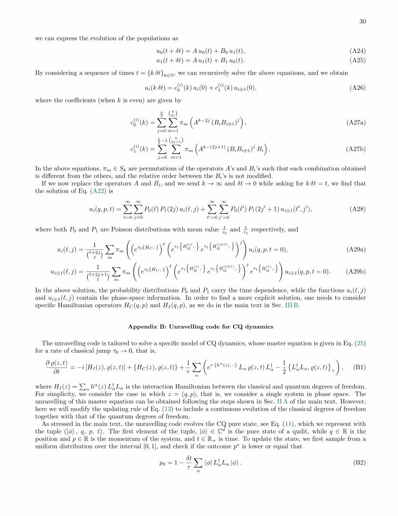
30

we can express the evolution of the populations as

u0(t+ δt) = Au0(t) +B0 u1(t), (A24)

u1(t+ δt) = Au1(t) +B1 u0(t). (A25)

By considering a sequence of times t = k δtk∈N, we can recursively solve the above equations, and we obtain

ui(k δt) = c(i)0 (k)ui(0) + c

(i)1 (k)ui⊕1(0), (A26)

where the coefficients (when k is even) are given by

c(i)0 (k) =

k2∑j=0

( k2j)∑m=1

πm

(Ak−2j (BiBi⊕1)

j), (A27a)

c(i)1 (k) =

k2−1∑j=0

( k2j+1)∑m=1

πm

(Ak−(2j+1) (BiBi⊕1)

jBi

). (A27b)

In the above equations, πm ∈ Sk are permutations of the operators A’s and Bi’s such that each combination obtainedis different from the others, and the relative order between the Bi’s is not modified.

If we now replace the operators A and Bi, and we send k → ∞ and δt → 0 while asking for k δt = t, we find thatthe solution of Eq. (A22) is

ui(q, p, t) =

∞∑`=0

∞∑j=0

P0(`)P1(2j)ui(`, j) +

∞∑`′=0

∞∑j′=0

P0(`′)P1(2j′ + 1)ui⊕1(`′, j′), (A28)

where both P0 and P1 are Poisson distributions with mean value tτ0

and tτ1

respectively, and

ui(`, j) =1(

`+2j`

) ∑m

πm

((eτ0HC ,·

)`(eτ1H

(i)Q ,·

eτ1H

(i⊕1)Q ,·

)j)ui(q, p, t = 0), (A29a)

ui⊕1(`, j) =1(

`+2j+1`

) ∑m

πm

((eτ0HC ,·

)`(eτ1H

(i)Q ,·

eτ1H

(i⊕1)Q ,·

)jeτ1H

(i)Q ,·

)ui⊕1(q, p, t = 0). (A29b)

In the above solution, the probability distributions P0 and P1 carry the time dependence, while the functions ui(`, j)and ui⊕1(`, j) contain the phase-space information. In order to find a more explicit solution, one needs to considerspecific Hamiltonian operators HC(q, p) and HI(q, p), as we do in the main text in Sec. III B.

Appendix B: Unravelling code for CQ dynamics

The unravelling code is tailored to solve a specific model of CQ dynamics, whose master equation is given in Eq. (25)for a rate of classical jump τ0 → 0, that is,

∂ %(z, t)

∂t= −i [HI(z), %(z, t)] + HC(z), %(z, t)+

1

τ

∑α

(eτ h

α(z), · Lα %(z, t)L†α −1

2

L†αLα, %(z, t)

+

), (B1)

where HI(z) =∑α h

α(z)L†αLα is the interaction Hamiltonian between the classical and quantum degrees of freedom.For simplicity, we consider the case in which z = (q, p), that is, we consider a single system in phase space. Theunravelling of this master equation can be obtained following the steps shown in Sec. II A of the main text. However,here we will modify the updating rule of Eq. (13) to include a continuous evolution of the classical degrees of freedomtogether with that of the quantum degrees of freedom.

As stressed in the main text, the unravelling code evolves the CQ pure state, see Eq. (11), which we represent withthe tuple (|φ〉 , q, p, t). The first element of the tuple, |φ〉 ∈ Cd is the pure state of a qudit, while q ∈ R is theposition and p ∈ R is the momentum of the system, and t ∈ R+ is time. To update the state, we first sample from auniform distribution over the interval [0, 1], and check if the outcome p? is lower or equal that

p0 = 1− δt

τ

∑α

〈φ|L†αLα |φ〉 . (B2)

31

If this is the case, that is, p? ≤ p0, we apply the continuous update to the CQ state, and we obtain the followingtuple, (

1√N0

(1− i δtHeff) |φ〉 , q +∂HC

∂pδt, p− ∂HC

∂qδt, t+ δt

), (B3)

where N0 is the normalisation of the updated quantum state, and Heff = HI(z) − i2τ

∑α L†αLα. If p? > p0, instead,

we randomly choose an α-jump according to the distribution,

pα =δt

τ〈φ|L†αLα |φ〉 , ∀α. (B4)

In this case, we evolve the state using the following update rule,(1√Nα

Lα |φ〉 , q +∂hα

∂pτ, p− ∂hα

∂qτ, t+ δt

), (B5)

where Nα is the normalisation of the new quantum state.It is worth noting that the updating rule of Eq. (B3) includes the continuous evolution of the classical degrees

of freedom, as opposed to the case shown in the main text, Eq. (13). This addition in the updating rule is due topresence, in the above master equation, of the Poisson bracket between the classical Hamiltonian HC and the CQstate. In fact, it is easy to see that the first order in δt of the phase space shift operator coincides with the action ofthe Poisson bracket, since for any (analytic) function f over the phase space we have

f

(q − ∂HC

∂pδt, p+

∂HC

∂qδt

)= e

δt(∂HC∂q

∂∂p−

∂HC∂p

∂∂q

)f(q, p) =

(1 + δt HC , · +O(δt2)

)f(q, p). (B6)

Using the above equation together with the fact that the unravelling provides a first order approximation of theevolution given by the master equation, one can show that the updating rule in this section correctly reproduces thedynamics of Eq. (B1).

The code for the CQ unravelling can be found on GitHub.