1

High Performance Algorithms for Multiple Streaming Time Series

Xiaojian ZhaoAdvisor: Dennis Shasha

Department of Computer ScienceCourant Institute of Mathematical Sciences

New York UniversityJan. 10 2006

2

Roadmap: Motivation Incremental Uncooperative Time Series Correlation Incremental Matching Pursuit (MP) (optional) Future Work and Conclusion

3

Motivation (1) Financial time series streams are watched closely by

millions of traders. “Which pairs of stocks were correlated with a value of over Which pairs of stocks were correlated with a value of over

0.9 for the last three hours? Report this information every h0.9 for the last three hours? Report this information every half houralf hour” (Incremental pairwise correlation)(Incremental pairwise correlation)

“How to form a portfolio consisting of a small set of stocks How to form a portfolio consisting of a small set of stocks which replicates the market? Update it every hour” (Increwhich replicates the market? Update it every hour” (Incremental matching pursuit)mental matching pursuit)

4

Motivation (2) As processors speed up, algorithmic efficiency no

longer matters … one might think. True if problem sizes stay same. But they don’t. As processors speed up, sensors improve

Satellites spewing out more data a day Magnetic resonance imagers give higher resolution

images, etc.

5

High performance incremental algorithms

Incremental Uncooperative Time Series Correlation Monitor and report the correlation information among all time

series incrementally (e.g. every half hour) Improve the efficiency from quadratic to super-linear

Incremental Matching Pursuit (MP) Monitor and report the approximation vectors of matching pursuit

incrementally (e.g. every hour) Improve the efficiency significantly

6

Incremental Uncooperative Time Series Correlation

7

Problem statement: Detect and report the correlation incrementally and

rapidly Extend the algorithm into a general engine Apply it in practical application domains

8

Online detection of high correlation

Correlated!

Correlated!

9

Pearson correlation and Euclidean distance

Normalized Euclidean distance Pearson correlation Normalization

dist2=2(1- correlation)

From now on, we will not differentiate between correlation and Euclidean distance

)var(

)(

sw

swii X

XavgXX

10

Naïve approach: pairwise correlation

Given a group of time series, compute the pairwise correlation

Time O(WN2), where

N : number of streams

W: window size (e.g. in the past one hour)

Let’s see high performance algorithms!

11

Technical review

Framework: GEMINI

Tools: Data Reduction Techniques

Deterministic Orthogonal vs. Randomized

Fourier Transform, Wavelet Transform, and Random Projection

Target: Various Data

Cooperative vs. Uncooperative

12

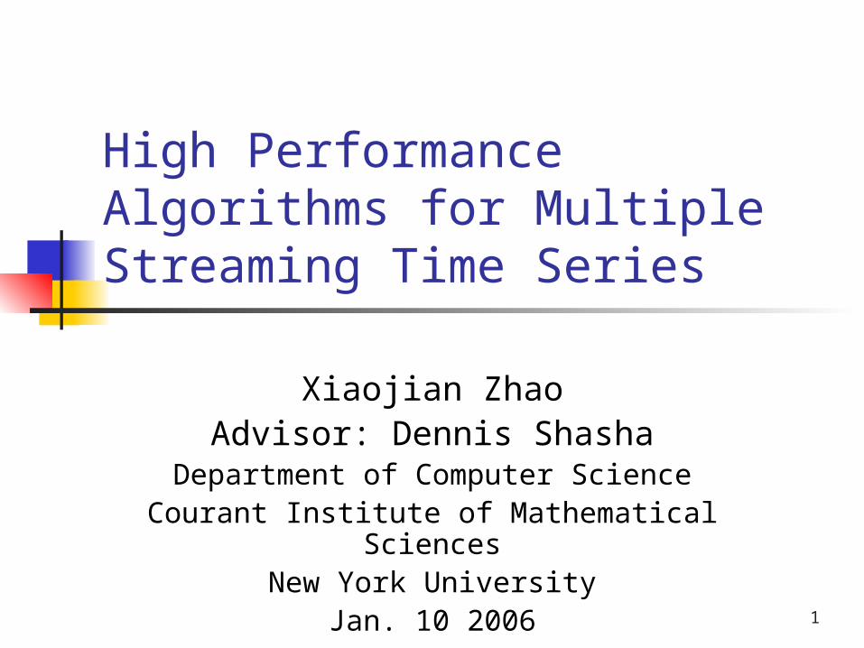
GEMINI Framework*

* Faloutsos, C., Ranganathan, M. & Manolopoulos, Y. (1994). Fast subsequence matching in time-series databases,. SIGMOD, 1994

Data reduction, e.g.

DFT, DWT, SVD

13

GEMINI: an example Objective: find the nearest neighborhood (L2-norm) of each time series. Compute the Fourier Transform over each of them, e.g. X and Y; yield

two coefficient vectors Xf and Yf

Xf=(a1, a2, …ak) and Yf=(b1, b2, …bk) Original distance vs. coefficient distance (Parseval's Theorem)

khwherebababa

bababa

yxyxyx

d

hh

kk

kk

2222

211

2222

211

2222

211

)()()(

)()()(

)()()(

||y-x||

Because, for some data types, energy concentrates on first a few frequency components, coefficient distance can work as a very good filter and at the same time guarantee no false negatives

They may be stored in a tree or grid structure

14

Random Walk

0

0.2

0.4

0.6

0.8

1

1.2

1 10 19 28 37 46 55 64 73 82 91 100

The number of coefficients

Ra

tio

ov

er

tota

l en

erg

y

ratio

DFT on random walk

2222

211

~

)()()( hh bababad

15

Review: DFT/DWT vs. Random Projection

Fourier Transform, Wavelet Transform and SVD A set of orthogonal base (deterministic)

Based on Parseval's Theorem Random Projection A set of random base (non-deterministic) Based on Johnson-Lindenstrauss (JL) Lemma

Orthogonal Base Random Base

16

Review: Random Projection: Intuition

You are walking in a sparse forest and you are lost. You have an outdated cell phone without a GPS (w/o latitude&altitude). You want to know if you are close to your friend. You identify yourself at 100 meters from Bestbuy and 200 meters from

a silver building etc. If your friend is at similar distances from several of these landmarks, y

ou might be close to one another. Random projections are analogous to these distances to landmarks.

17

),...,,,( 11312111 wrrrrR

),...,,,( 22322212 wrrrrR ),...,,,( 33332313 wrrrrR ),...,,,( 44342414 wrrrrR

),,,( 4321 xskxskxskxsk

),,,( 4321 yskyskyskysk

inner product

random vector

sketches

time series

Random Projection

),...,,( 321 wxxxxx

),...,,( 321 wyyyyy

Sketch: A vector of output returned by random projection

18

Review: Sketch Guarantees *

Johnson-Lindenstrauss ( JL) Lemma: For any and any integer n, let k be a positive integer such that

Then for any set V of n points in , there is a map such that for all

Further this map can be found in randomized polynomial time

10

dR kd RRf :Vvu ,

222 ||||)1(||)()(||||||)1( vuvfufvu

•W.B.Johnson and J.Lindenstrauss. “Extensions of Lipshitz mapping into hilbert space”. Contemp. Math.,26:189-206,1984

nk ln)3/2/(4 132

19

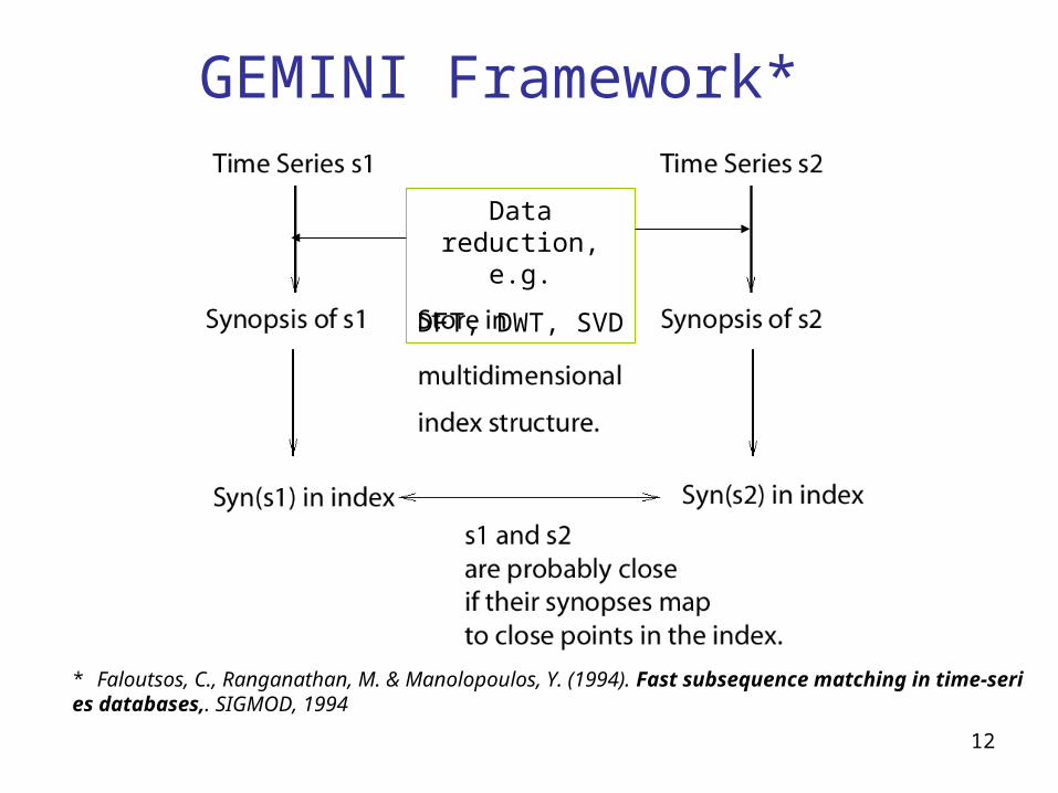
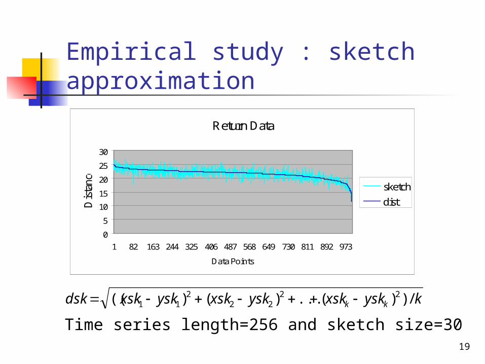
Empirical study : sketch approximation

Return Data

0

5

10

15

20

25

30

1 82 163 244 325 406 487 568 649 730 811 892 973

Data Points

Dis

tanc

e

sketch

dist

kyskxskyskxskyskxskdsk kk /))(...)()(( 2222

211

Time series length=256 and sketch size=30

20

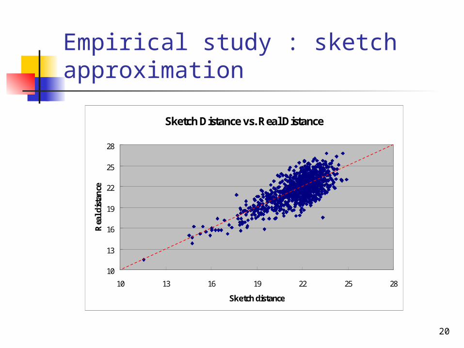
Empirical study : sketch approximation

Sketch Distance vs. Real Distance

10

13

16

19

22

25

28

10 13 16 19 22 25 28

Sketch distance

Rea

l dis

tan

ce

21

Empirical study: sketch distance/real distance

Factor distribution

0%

1%

2%

3%

4%

5%

Factor(Real distance/Sketch distance)

Per

cent

age

of d

ista

nce

number

Factor distribution

0%

1%

2%

3%

4%

5%

6%

7%

1.25

1.20

1.16

1.12

1.09

1.05

1.02

0.99

0.96

0.93

0.91

0.88

Factor(Real distance/Sketch distance)

Per

cent

age

of d

ista

nce

number

Sketch=30

Sketch=80

Factor distribution

0%

2%

4%

6%

8%

10%

12%

1.19

1.16

1.14

1.11

1.09

1.06

1.04

1.02

1.00

0.98

0.96

0.94

0.93

Factor(Real distance/Sketch distance)

Per

cent

age

of d

ista

nce

number

Sketch=1000

22

Data classification

Cooperative Time series exhibiting a fundamental degree of regularity,

allowing them to be represented by the first few coefficients in the spectral space with little loss of information

Example: Stock Price (random walk) Tools: Fourier Transform, Wavelet Transform, SVD

Uncooperative Time series whose energy is not concentrated in only a few

frequency components, e.g. Example: Stock Return (= ) Tool: Random Projection

pricesyesterday

pricesyesterdaypricestoday

'

''

23

Random Walk

0

0.2

0.4

0.6

0.8

1

1.2

1 10 19 28 37 46 55 64 73 82 91 100

The number of coefficients

Ra

tio

ov

er

tota

l en

erg

y

ratio

White Noise

00.10.20.30.40.50.60.70.80.9

1 9 17 25 33 41 49 57 65 73 81 89 97

The number of coefficients

Rat

io o

ver

tota

l en

erg

yratio

DFT on random walk and white noise

Cooperative

Uncooperative

24

Approximation Power: SVD Distance vs. Sketch Distance

Comparison over Return Data

0

5

10

15

20

25

30

0 100 200 300 400 500 600 700 800 900

Data Points

Dis

tanc

e Real Dist

Sketch

SVD

•Note: SVD is superior to DFT and DWT in approximation power.

•But all of them are all bad for uncooperative data.

•Here sketch size = 32 and SVD coefficient number =30

25

Our new algorithm*

• The big picture of the system

• Structured random vector (New)

• Compute sketch by structured convolution (New)

• Optimize in the parameter space (New)

• Empirical study

•Richard Cole, Dennis Shasha and Xiaojian Zhao. “Fast Window Correlations Over Uncooperative Time Series”. SIGKDD 2005

26

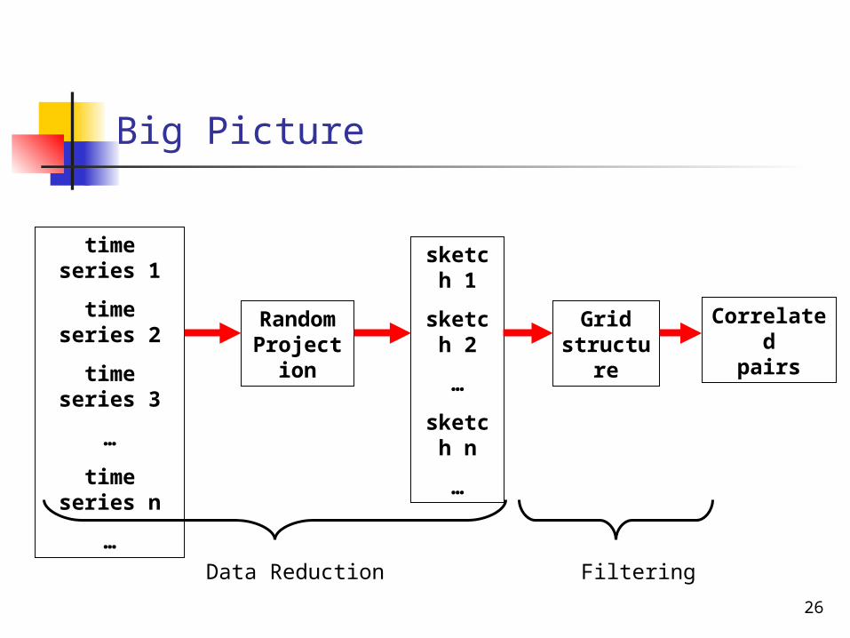
Big Picture

Random Projection

time series 1

time series 2

time series 3

…

time series n

…

sketch 1

sketch 2

…

sketch n

…

Grid structure

Correlatedpairs

Data Reduction Filtering

27

Our objective reminded

Monitor and report the correlation periodically e.g. “every half hour”

We chose Random Projection as a means to reduce the data dimension

The time series needs to be looked at in a time window. This time window should slide forward as time goes on.

28

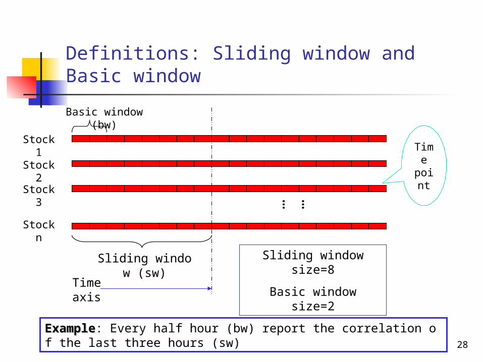
Definitions: Sliding window and Basic window

Time axis

……

Stock 1

Stock 2

Stock 3

Stock n

Sliding window (sw)

Sliding window size=8

Basic window size=2

Basic window (bw)

Time

point

ExampleExample: Every half hour (bw) report the correlation of the last three hours (sw)

29

Random vector and naïve random projection

Choose randomly sw random numbers to form a random vector R=(r1, r2, r3, r4, r5, r6, r7, r8, r9, r10, r11, r12)

Inner product starts from each data pointXsk1=(x1 x2 x3 x4 x5 x6 x7 x8 x9 x10 x11 x12)*R

Xsk2=(x2 x3 x4 x5 x6 x7 x8 x9 x10 x11 x12 x13)*R

Xsk3=(x3 x4 x5 x6 x7 x8 x9 x10 x11 x12 x13 x14)*R

……

We improve it in two ways

Partition a random vector of length sw into several basic windows

Use convolution instead of inner product

30

How to construct a random vectorConstruct a random vector of 1/-1 of length sw.

Suppose sliding window size=12, and basic window size=4

The random vector within a basic window is

A control vector

A final complete random vector for a sliding window may look like:

),,,( 4321 rrrrRbw

2

11/1 probwithri

2

11/1),,( 321 probwithbbbbb i

(1 1 -1 1; -1 -1 1 -1; 1 1 -1 1)Here Rbw=(1 1 -1 1) b=(1 -1 1)

Rbw -Rbw Rbw

31

Naive algorithm and hope for improvement

There is redundancy in the second dot product given the first one. We will eliminate the repeated computation to save time

dot product

r=( 1 1 -1 1 ; -1 -1 1 -1; 1 1 -1 1 )

x=(x1 x2 x3 x4; x5 x6 x7 x8; x9 x10 x11 x12)xsk=r*x= x1+x2-x3+x4-x5-x6+x7-x8+x9+x10-x11+x12

With new data point arrival, this operation will be done again

r= ( 1 1 -1 1 ; -1 -1 1 -1; 1 1 -1 1 ) x’=(x5 x6 x7 x8 ; x9 x10 x11 x12; x13 x14 x15 x16)

xsk=r*x’= x5+x6-x7+x8-x9-x10+x11+x12+x13+x14+x15- x16*

32

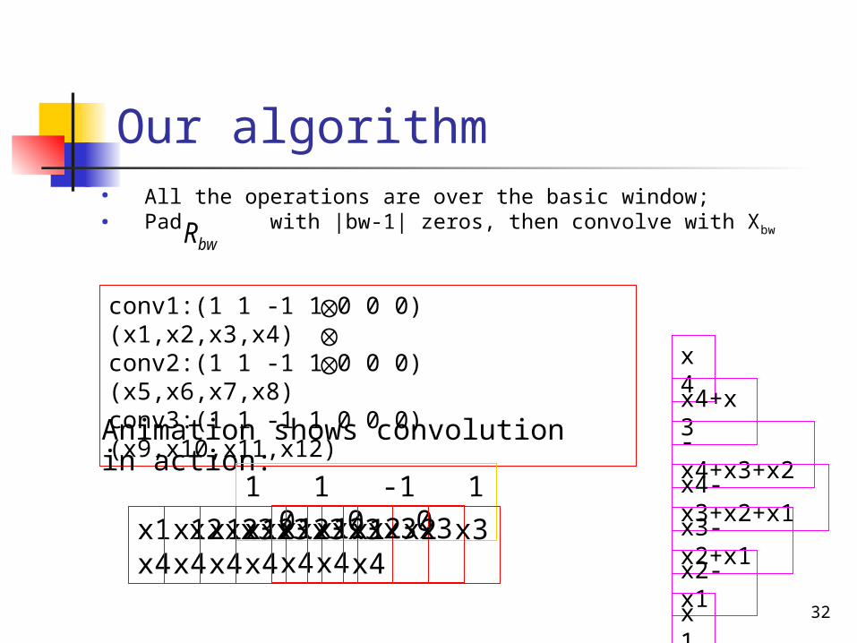
conv1:(1 1 -1 1 0 0 0) (x1,x2,x3,x4)conv2:(1 1 -1 1 0 0 0) (x5,x6,x7,x8)conv3:(1 1 -1 1 0 0 0) (x9,x10,x11,x12)

Our algorithm● All the operations are over the basic window;● Pad with |bw-1| zeros, then convolve with Xbw bwR

Animation shows convolution in action:

1 1 -1 1 0 0 0

x1 x2 x3 x4

x4

x4+x3

-x4+x3+x2

x4-x3+x2+x1

x3-x2+x1

x2-x1

x1

x1 x2 x3 x4x1 x2 x3 x4x1 x2 x3 x4x1 x2 x3 x4x1 x2 x3 x4x1 x2 x3 x4

33

Our algorithm: example

+

First Convolution Second Convolution Third Convolution

x4

x4+x3

x2+x3-x4

x1+x2-x3+x4

x1-x2+x3

x2-x1

x1

x8

x8+x7

x6+x7-x8

x5+x6-x7+x8

x5-x6+x7

x6-x5

x5

x12

x12-x11

x10+x11-x12

x9+x10-x11+x12

x9-x10+x11

x10-x9

x9

+

xsk1= (x1+x2-x3+x4)-(x5+x6-x7+x8)+(x9+x10-x11+x12)xsk2=(x2+x3-x4+x5)-(x6+x7-x8+x9)+(x10+x11-x12+x13)

34

Our algorithm: example

(Sk1 Sk5 Sk9)*(b1 b2 b3) * is inner product

sk2=(x2+x3-x4) + (x5)sk6=(x6+x7-x8) + (x9)sk10=(x10+x11-x12) + (x13)Then sum up and we havexsk2=(x2+x3-x4+x5)-(x6+x7-x8+x9)+(x10+x11-x12+x13)b=( 1 -1 1)

sk1=(x1+x2-x3+x4)sk5=(x5+x6-x7+x8) sk9=(x9+x10-x11+x12)xsk1= (x1+x2-x3+x4)-(x5+x6-x7+x8)+(x9+x10-x11+x12)b= ( 1 -1 1)

First sliding window

Second sliding window

35

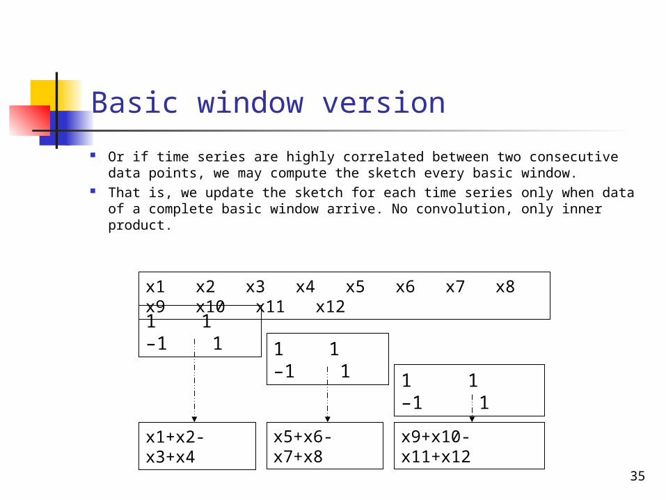
Basic window version

Or if time series are highly correlated between two consecutive data points, we may compute the sketch every basic window.

That is, we update the sketch for each time series only when data of a complete basic window arrive. No convolution, only inner product.

1 1 –1 1

x1 x2 x3 x4 x5 x6 x7 x8 x9 x10 x11 x12

1 1 –1 1

1 1 –1 1

x1+x2-x3+x4 x5+x6-x7+x8 x9+x10-x11+x12

36

Overview of our new algorithm

The projection of a sliding window is decomposed into operations over basic windows

Each basic window is convolved/inner product with each random vector only once

We may provide the sketches starting from each data point or starts from the beginning of each basic window.

There is no redundancy.

37

Performance comparison

Naïve algorithm For each datum and random vector (1) O(|sw|) integer additions Pointwise version

Asymptotically for each datum and random vector(1) O(|sw|/|bw|) integer additions(2) O(log |bw|) floating point operations (use FFT in computing convolutions)

Basic window versionAsymptotically for each datum and random vectorO(|sw|/|bw|2) integer additions

38

Big picture revisited

Random Projection

time series 1

time series 2

time series 3

…

time series n

…

sketch 1

sketch 2

…

sketch n

…

Grid structure

Correlatedpairs

Filtering

So far we reduce the data dimension efficiently. Next, how can it be used as a filter?

39

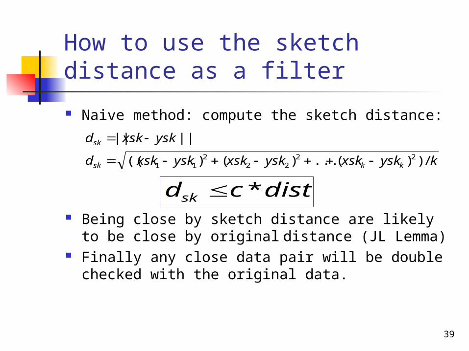
How to use the sketch distance as a filter

Naive method: compute the sketch distance:

Being close by sketch distance are likely to be close by original distance (JL Lemma)

Finally any close data pair will be double checked with the original data.

kyskxskyskxskyskxskd

yskxskd

kksk

sk

/))(...)()((

||||

2222

211

distcdsk *

40

Use the sketch distance as a filter

But we do not use it, why? Expensive. Since we still have to do the pairwise comparison be

tween each pair of stocks which is , k is the size of the sketches, e.g. typically 30, 40, etc

Let’s see our new strategy

)( 2knO

41

Our method: sketch unit distance

)8,7,6,5,4,3,2,1( xskxskxskxskxskxskxskxskxsk )8,7,6,5,4,3,2,1( yskyskyskyskyskyskyskyskysk

|11| yskxsk |22| yskxsk |33| yskxsk |44| yskxsk |55| yskxsk |66| yskxsk |77| yskxsk |88| yskxsk

Given sketches:

If f distance chunks have we may say where: f: 30%, 40%, 50%, 60% … c: 0.8, 0.9, 1.1…

distcyskixski *|| distyx ||||

We have

42

Further: sketch groups

||||

,,, 321

gigigi

ggg

yskxskdsk

where

dskdskdsk

4/))()()()(( 244

233

222

2111 yskxskyskxskyskxskyskxskdskg

...)8,7,6,5,4,3,2,1( xskxskxskxskxskxskxskxskxsk ...)8,7,6,5,4,3,2,1( yskyskyskyskyskyskyskyskysk

We may compute the sketch group:

For example

If f sketch groups have we may say distcdskdsk gigi *|| distyx ||||

Remind us of a grid

structure

43

Grid structure To avoid checking all pairs, we can use a grid structure

and look in the neighborhood, this will return a super set of highly correlated pairs.

The data labeled as “potential” will be double checked using the raw data vectors.

),...,( 21 kxxxx

44

Optimization in parameter space

We will choose the best one to be applied to the practical data. But how? --- an engineering problem

Combinatorial Design (CD) Bootstrapping

How to choose the parameters g, c, f, N?

N: total number of the sketchesg: group sizec: the factor of distancef: the fraction of groups which are necessary to claim that two time series are close enough

Now, Let’s put all together.

45

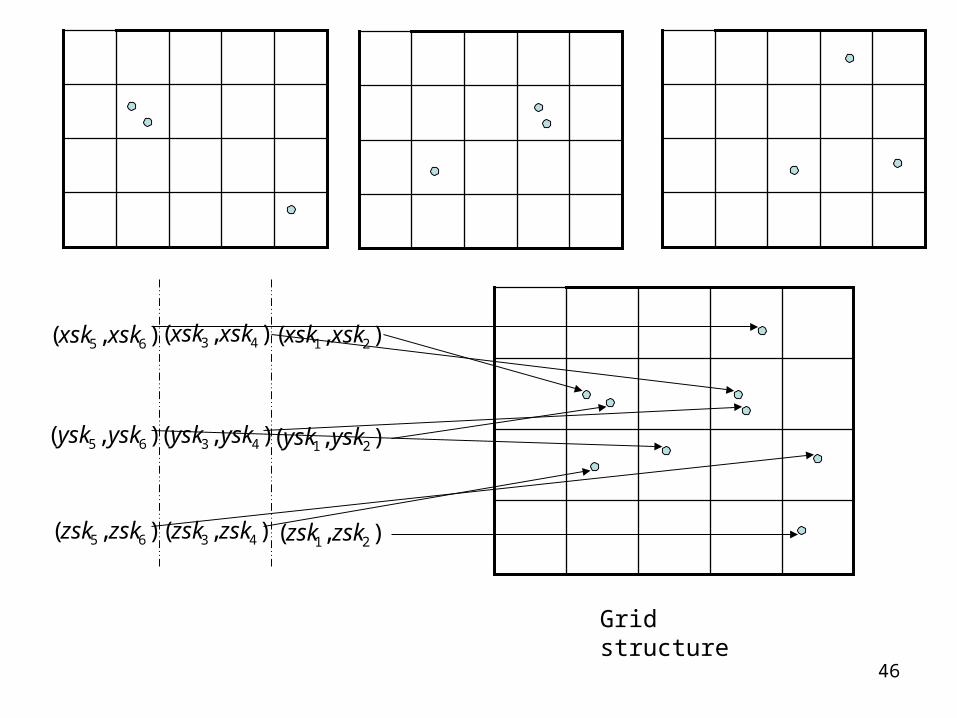
Inner product with random vectors r1,r2,r3,r4,r5,r6

),,,,,( 654321 xskxskxskxskxskxsk

),,,,,( 654321 yskyskyskyskyskysk

),,,,,( 654321 zskzskzskzskzskzsk

X Y Z

46

),( 21 xskxsk

),( 21 yskysk

),( 21 zskzsk

),( 43 xskxsk

),( 43 yskysk

),( 43 zskzsk

),( 65 xskxsk

),( 65 yskysk

),( 65 zskzsk

Grid structure

47

Empirical study: various data sources

Cstr: Continuous stirred tank reactor

Fortal_ecg: Cutaneous potential recordings of a pregnant woman

Steamgen: Model of a steam generator at Abbott Power Plant in Champaign IL

Winding: Data from a test setup of an industrial winding process

Evaporator: Data from an industrial evaporator

Wind: Daily average wind speeds for 1961-1978 at 12 synoptic meteorological stations in the Republic of Ireland

Spot_exrates: The spot foreign currency exchange rates

EEG: Electroencepholgram

48

Empirical study: performance comparison Comparison of Processing Time

0

0.2

0.4

0.6

0.8

1

1.2

price

retu

rn

evap

orat

or

spot

_exr

ates

windin

gcs

tr eeg

foet

al_ec

g

steam

gen

wind

Practical Data Sets

Nor

mal

ized

Tim

e r

sketchdftscan

Sliding window=3616, basic window=32 and sketch size=60

49

Section conclusion

How to perform data reduction over uncooperative time series efficiently in contrast to well-established methods for cooperative data

How to cope with middle-size sketch vectors systematically. Sketch vector partition, grid structure Parameter space optimization by combinatorial design and

bootstrapping

Many ideas can be extended to other applications

50

Incremental Matching Pursuit (MP)

51

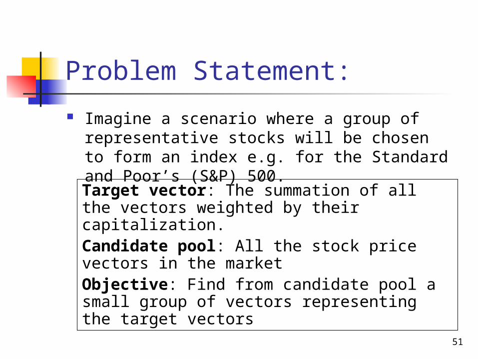
Problem Statement:

Imagine a scenario where a group of representative stocks will be chosen to form an index e.g. for the Standard and Poor’s (S&P) 500.

Target vector: The summation of all the vectors weighted by their capitalization.Candidate pool: All the stock price vectors in the market Objective: Find from candidate pool a small group of vectors representing the target vectors

52

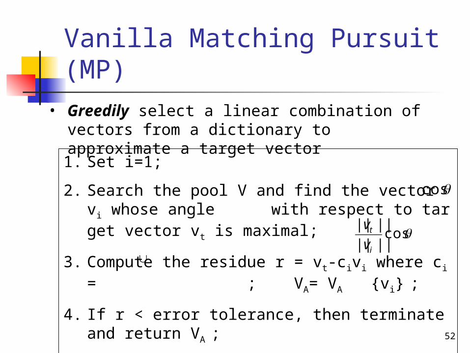
1. Set i=1;

2. Search the pool V and find the vector vi whose angle with respect to target vector vt is maximal;

3. Compute the residue r = vt-civi where ci = ; VA

= VA {vi} ;

4. If r < error tolerance, then terminate and return VA ;

5. Else set i = i + 1 and vt = r, go back to 2 ;

Vanilla Matching Pursuit (MP)

• Greedily select a linear combination of vectors from a dictionary to approximate a target vector

cos

cos||||

||||

i

t

v

v

53

v1

v2

v3

vt

54

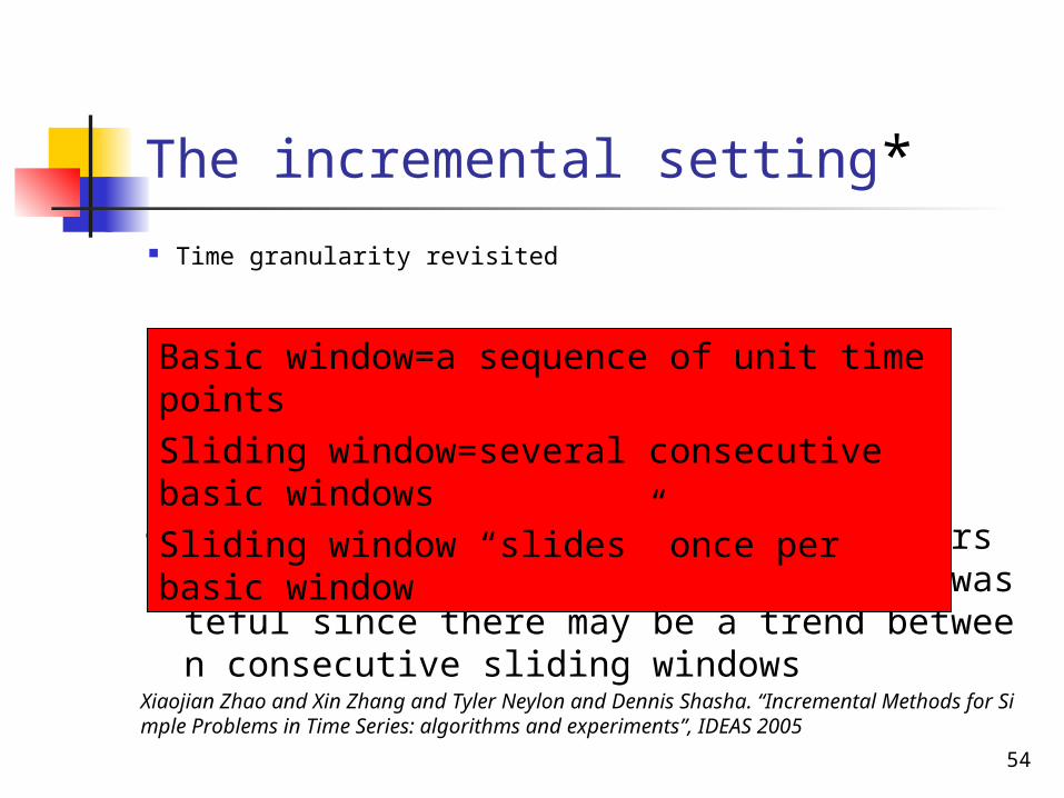
The incremental setting*

Time granularity revisited

• Recomputing the representative vectors entirely for each sliding window is wasteful since there may be a trend between consecutive sliding windows

Basic window=a sequence of unit time points

Sliding window=several consecutive basic windows

Sliding window “slides” once per basic window

Xiaojian Zhao and Xin Zhang and Tyler Neylon and Dennis Shasha. “Incremental Methods for Simple Problems in Time Series: algorithms and experiments”, IDEAS 2005

55

First idea: reuse vectors

The representative vectors may change only slightly in both components and their order

True only if basic window is sufficiently small e.g. 2, 3 time points

However, any newly introduced representative vector may alter the entire tail of the approximation path

The relative importance of the same representative vector may differ a lot from one sliding window to the next

56

Two insightful observations

The representative vectors are likely to remain the same within a few sliding windows, though the order may change

The vector of angles keeps quite consistent, i.e. ( , , ,…).

Here is the cosine of angle between the ith residue and the selected vector at that round.

An example is (0.9, 0.8, 0.7, 0.7, 0.6, 0.6, 0.6,…..)

cos

1cos 2cos 3cos

icos

57

Angle space exploration ( )

Whenever a vector is found whose is larger than some threshold, choose that vector.

If there is no such vector, the vector with largest is selected as the representative vector at this round.

cos

|cos|

|cos|

58

Second idea: cache good vectors

Those representative vectors appearing in the last several sliding windows form a cache C

The search for a representative vector starts from C. If not found then go to whole pool V

Works well in practice.

59

Empirical study: time comparison

Time Comparison

0

0.2

0.4

0.6

0.8

1

1.2

bw/power ratio

time

ratio

Incremental MP

Naive MP

60

Approximation Power Comparison

0

0.2

0.4

0.6

0.8

1

1.2

1.4

1.6

bw/power ratio

vect

or n

umbe

r ra

tio

Incremental MPNaive MP

Empirical study: approximation power comparison

61

Future Work and Conclusion

62

Future work: Anomaly Detection

Measure the relative distance of each point from its nearest neighbors

Our approach may serve as a monitor by reporting those points far from any normal points

63

Conclusion

1. Motivation2. Introduce the concept of cooperative vs. uncooperative

time series3. Propose a set of strategies dealing with different data

(Random projection, Structured Convolution, Combinatorial Design, Bootstrapping, Grid Structure)

4. Explore various incremental schemes Filter away obvious irrelevancies Reuse previous results.

5. Future Work

64

Thanks a lot!