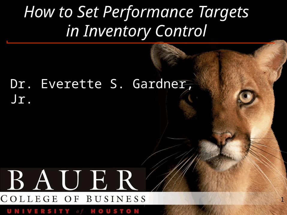
1

How to Set Performance Targets

in Inventory Control

Dr. Everette S. Gardner, Jr.

2

How to Set Performance Targets in Inventory Control

Clean up the parts list Develop a basic forecasting system Use the forecasts to classify parts (ABC+) Decide what to stock Decide where to stock it Divide the inventory into control groups:

JIT, MRP, EOQ, Annual buy

Develop benchmark performance measures

3

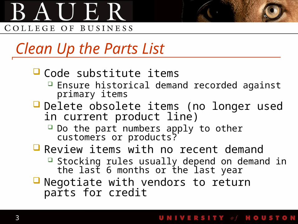
Clean Up the Parts List Code substitute items

Ensure historical demand recorded against primary items Delete obsolete items (no longer used in current

product line) Do the part numbers apply to other customers or

products? Review items with no recent demand

Stocking rules usually depend on demand in the last 6 months or the last year

Negotiate with vendors to return parts for credit

4

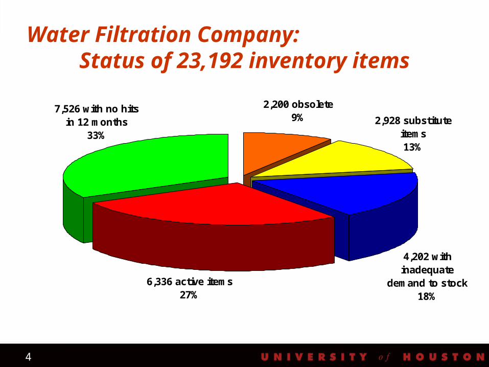
Water Filtration Company: Status of 23,192 inventory items

4,202 with inadequate

demand to stock18%

2,928 substitute items13%

2,200 obsolete9%

7,526 with no hits in 12 months

33%

6,336 active items27%

5

The Importance of Forecasting

Forecasts determine production and inventory quantities MRP: Master schedule EOQ: Order quantity, leadtime demand, safety stock JIT: Requirements to internal and external suppliers

6

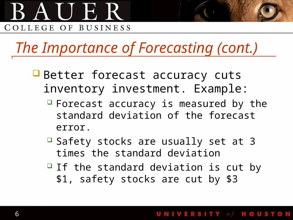
The Importance of Forecasting (cont.) Better forecast accuracy cuts inventory

investment. Example: Forecast accuracy is measured by the standard

deviation of the forecast error. Safety stocks are usually set at 3 times the standard

deviation If the standard deviation is cut by $1, safety stocks

are cut by $3

7

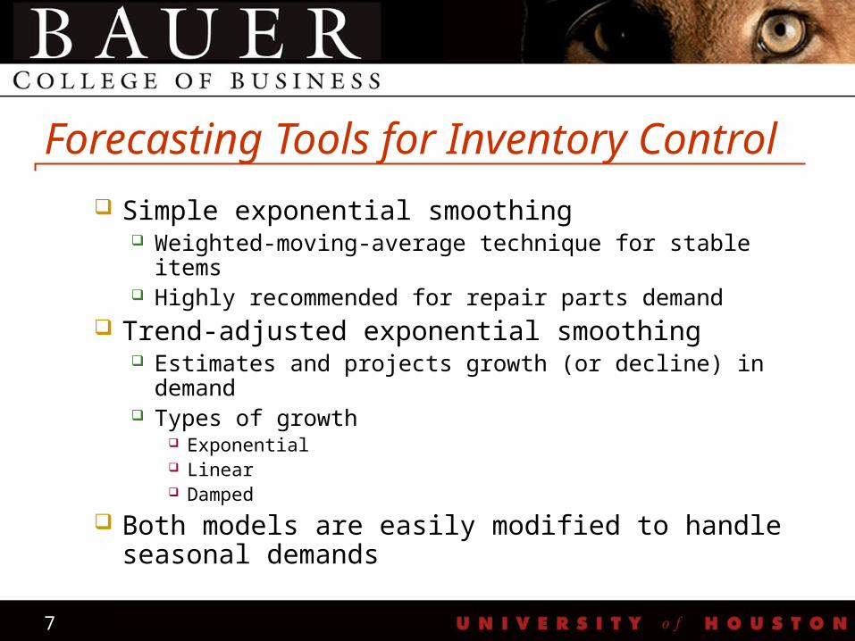
Forecasting Tools for Inventory Control Simple exponential smoothing

Weighted-moving-average technique for stable items Highly recommended for repair parts demand

Trend-adjusted exponential smoothing Estimates and projects growth (or decline) in demand Types of growth

Exponential Linear Damped

Both models are easily modified to handle seasonal demands

8

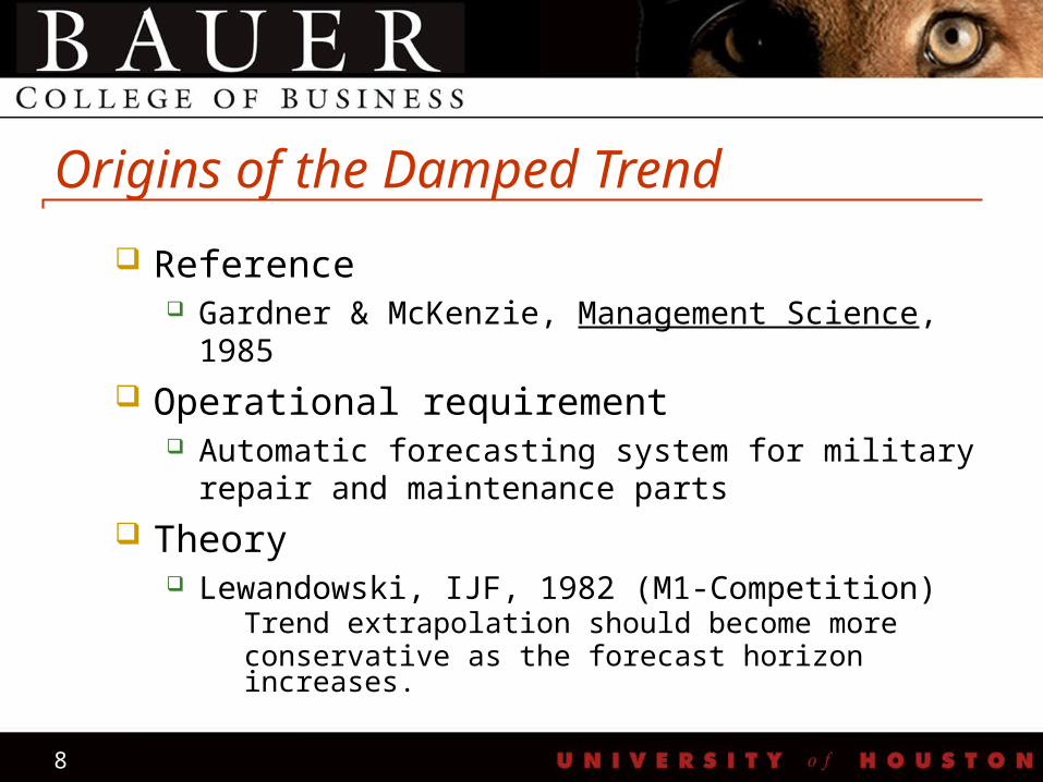
Origins of the Damped Trend

Reference Gardner & McKenzie, Management Science, 1985

Operational requirement Automatic forecasting system for military repair and

maintenance parts

Theory Lewandowski, IJF, 1982 (M1-Competition)

Trend extrapolation should become moreconservative as the forecast horizon increases.

9

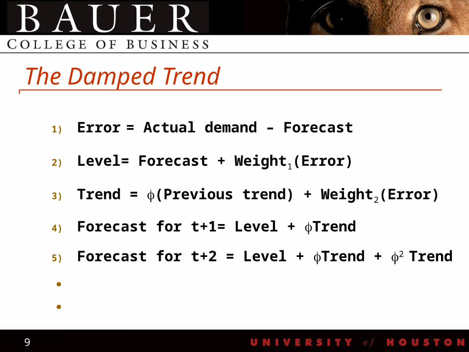
The Damped Trend

1) Error = Actual demand – Forecast

2) Level= Forecast + Weight1(Error)

3) Trend = (Previous trend) + Weight2(Error)

4) Forecast for t+1= Level + Trend

5) Forecast for t+2 = Level + Trend + 2 Trend

.

.

10

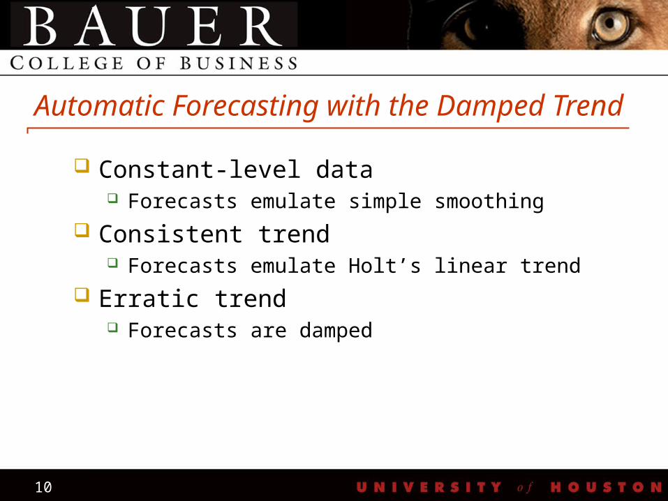
Automatic Forecasting with the Damped Trend Constant-level data

Forecasts emulate simple smoothing

Consistent trend Forecasts emulate Holt’s linear trend

Erratic trend Forecasts are damped

11

26

27

28

29

30

31

32

33

34

35

36

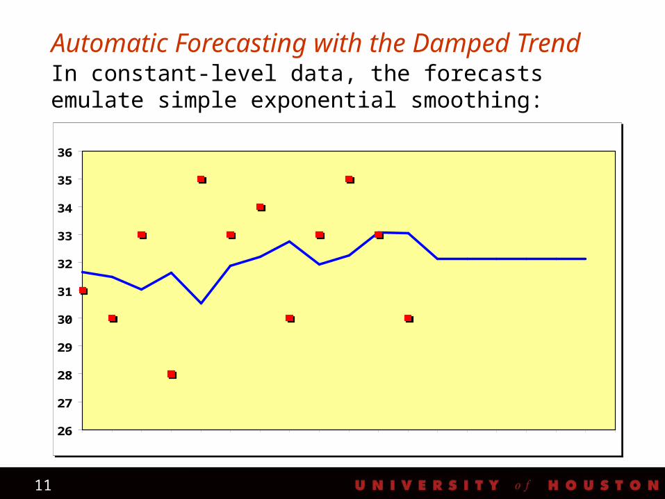
Automatic Forecasting with the Damped TrendIn constant-level data, the forecasts emulate simple exponential smoothing:

12

20

25

30

35

40

45

50

55

60

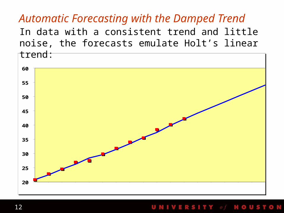
In data with a consistent trend and little noise, the forecasts emulate Holt’s linear trend:

Automatic Forecasting with the Damped Trend

13

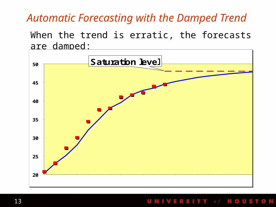
Automatic Forecasting with the Damped Trend

When the trend is erratic, the forecasts are damped:

20

25

30

35

40

45

50 Saturation level

14

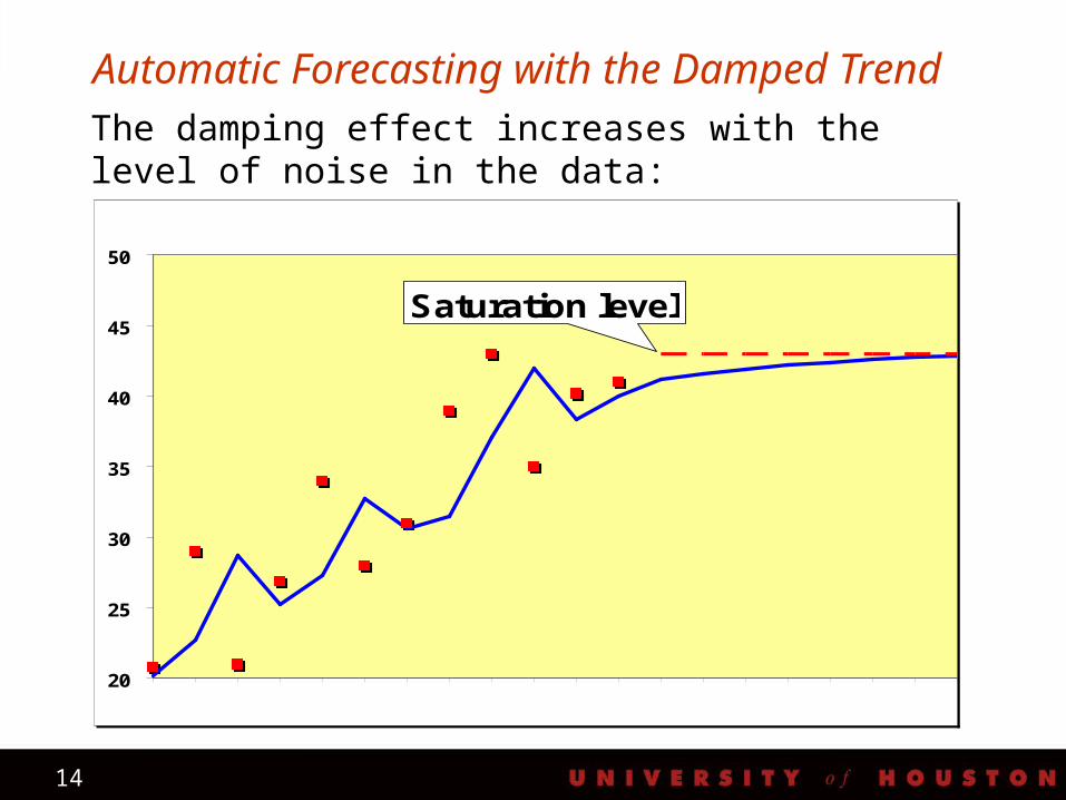
Automatic Forecasting with the Damped TrendThe damping effect increases with the level of noise in the data:

20

25

30

35

40

45

50

Saturation level

15

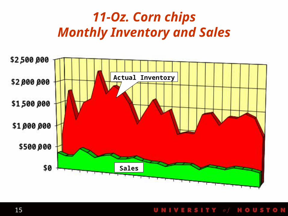
11-Oz. Corn chipsMonthly Inventory and Sales

Actual Inventory

Sales

16

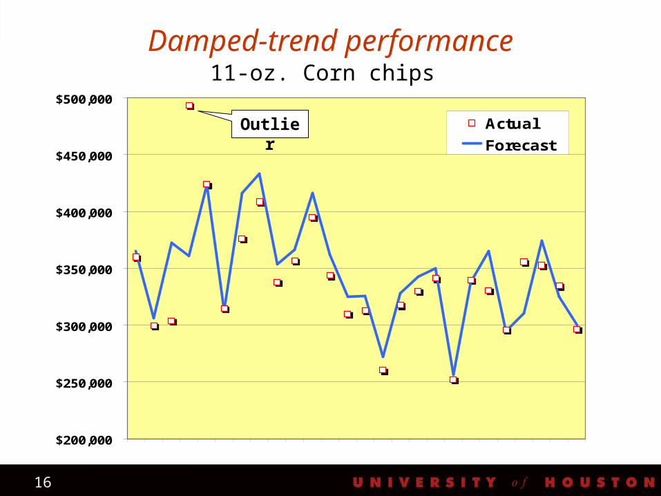
Damped-trend performance11-oz. Corn chips

$200,000

$250,000

$300,000

$350,000

$400,000

$450,000

$500,000

Actual

ForecastOutlier

17

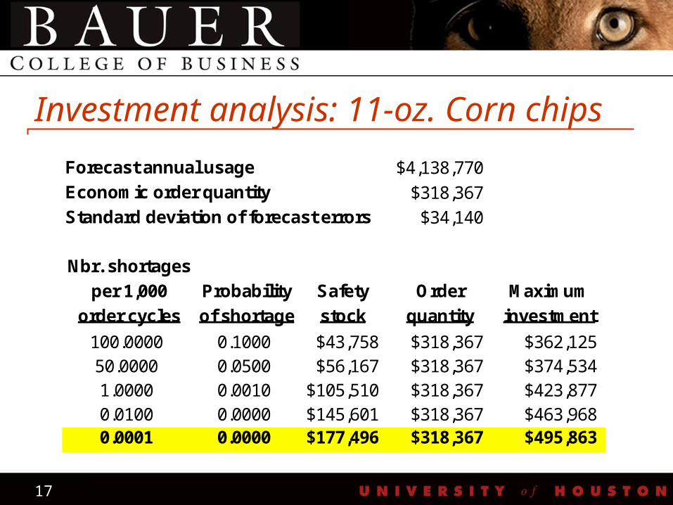
Investment analysis: 11-oz. Corn chipsForecast annual usage $4,138,770

Economic order quantity $318,367

Standard deviation of forecast errors $34,140

Nbr. shortages

per 1,000 Probability Safety Order Maximum

order cycles of shortage stock quantity investment

100.0000 0.1000 $43,758 $318,367 $362,12550.0000 0.0500 $56,167 $318,367 $374,5341.0000 0.0010 $105,510 $318,367 $423,8770.0100 0.0000 $145,601 $318,367 $463,9680.0001 0.0000 $177,496 $318,367 $495,863

18

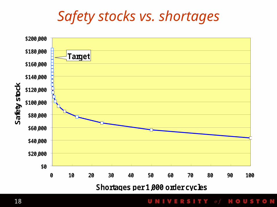
Safety stocks vs. shortages

$0

$20,000

$40,000

$60,000

$80,000

$100,000

$120,000

$140,000

$160,000

$180,000

$200,000

0 10 20 30 40 50 60 70 80 90 100

Shortages per 1,000 order cycles

Saf

ety

stoc

k

Target

19

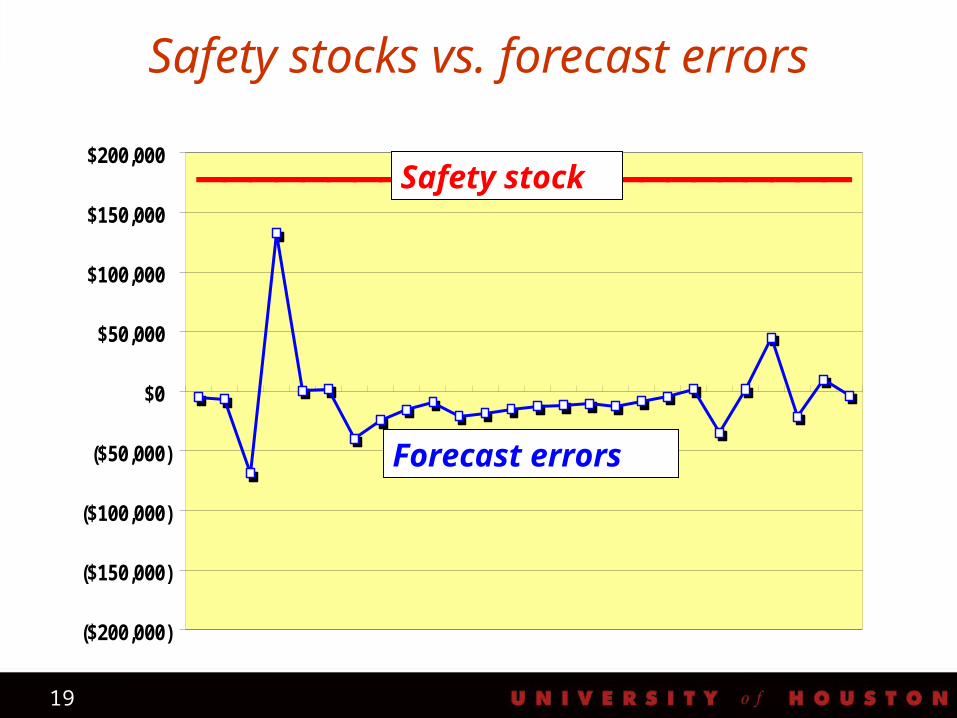
Safety stocks vs. forecast errors

($200,000)

($150,000)

($100,000)

($50,000)

$0

$50,000

$100,000

$150,000

$200,000Safety stock

Forecast errors

20

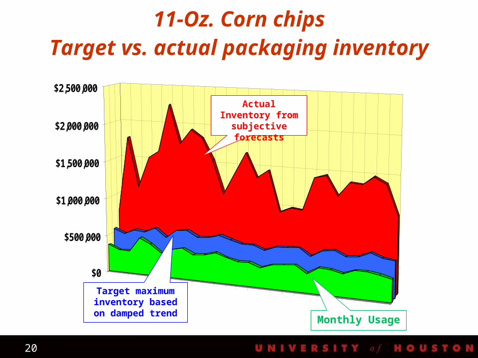
11-Oz. Corn chipsTarget vs. actual packaging inventory

Actual Inventory from

subjective forecasts

Month

$0

$500,000

$1,000,000

$1,500,000

$2,000,000

$2,500,000

Target maximum inventory based on damped trend

Actual Inventory from

subjective forecasts

Monthly Usage

21

How to forecast regional demand

Forecast total units with the damped trend

Forecast regional percentages with simple exponential smoothing

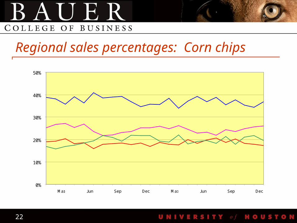
22

Regional sales percentages: Corn chips

0%

10%

20%

30%

40%

50%

Mar Jun Sep Dec Mar Jun Sep Dec

South

West

North

East

23

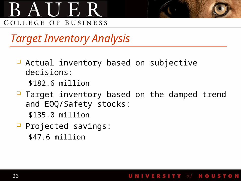
Target Inventory Analysis

Actual inventory based on subjective decisions:$182.6 million

Target inventory based on the damped trend and EOQ/Safety stocks:$135.0 million

Projected savings:$47.6 million

24

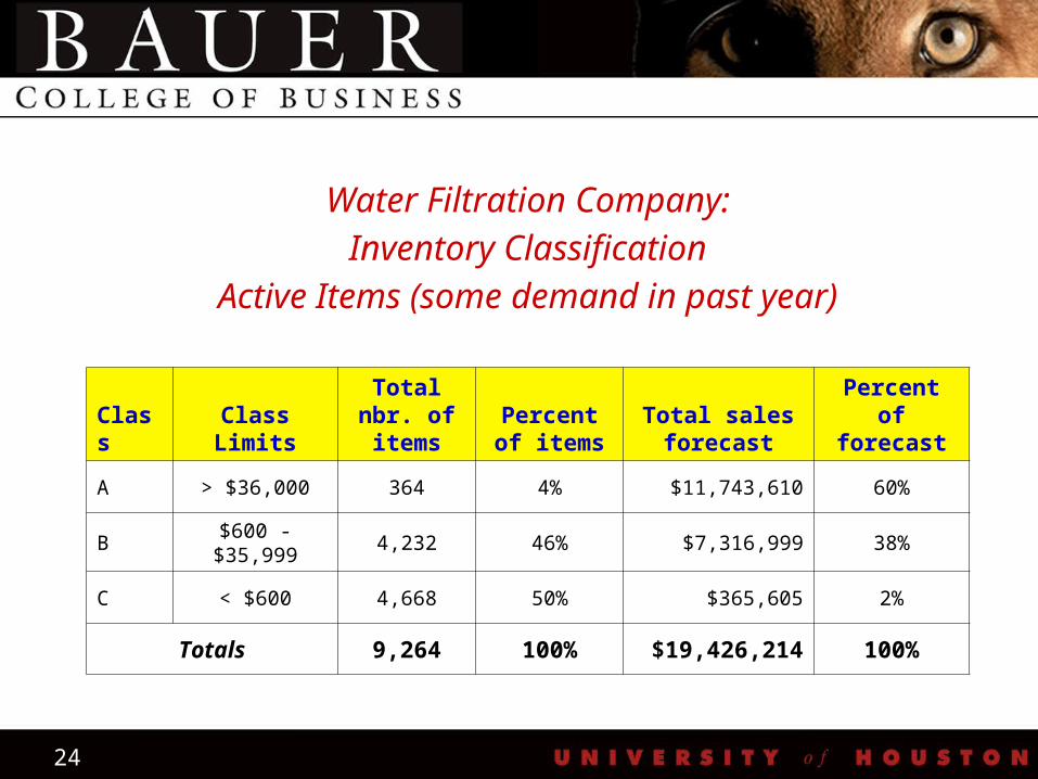
Water Filtration Company:Inventory Classification

Active Items (some demand in past year)

Class Class LimitsTotal nbr. of items

Percent of items

Total sales forecast

Percent of forecast

A > $36,000 364 4% $11,743,610 60%

B $600 - $35,999 4,232 46% $7,316,999 38%

C < $600 4,668 50% $365,605 2%

Totals 9,264 100% $19,426,214 100%

25

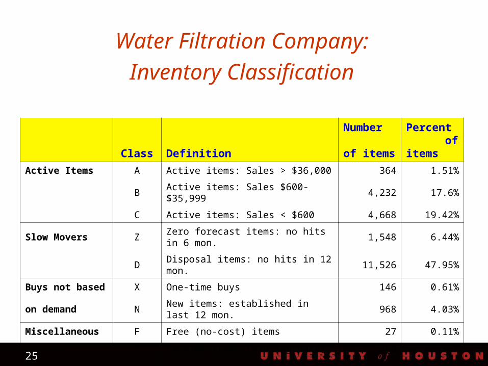
Water Filtration Company:

Inventory Classification

Class Definition

Number of items

Percent of items

Active Items A Active items: Sales > $36,000 364 1.51%

B Active items: Sales $600-$35,999 4,232 17.6%

C Active items: Sales < $600 4,668 19.42%

Slow Movers Z Zero forecast items: no hits in 6 mon. 1,548 6.44%

D Disposal items: no hits in 12 mon. 11,526 47.95%

Buys not based X One-time buys 146 0.61%

on demand N New items: established in last 12 mon. 968 4.03%

Miscellaneous F Free (no-cost) items 27 0.11%

P Problem items (missing data) 560 2.33%

Totals 24,039 100.0%

26

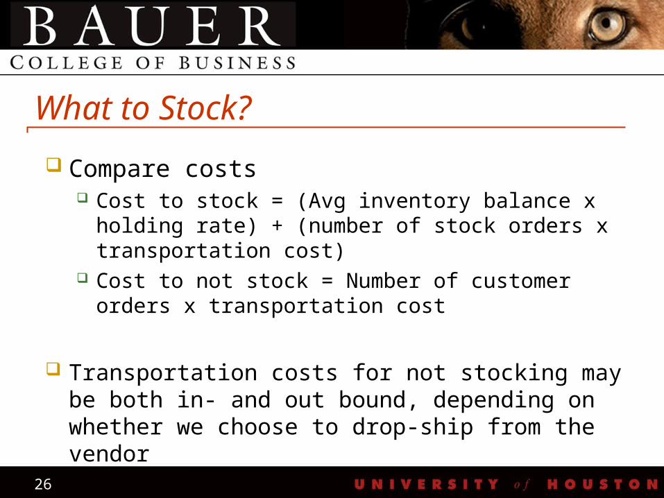
What to Stock?

Compare costs Cost to stock = (Avg inventory balance x holding rate)

+ (number of stock orders x transportation cost) Cost to not stock = Number of customer orders x

transportation cost

Transportation costs for not stocking may be both in- and out bound, depending on whether we choose to drop-ship from the vendor

27

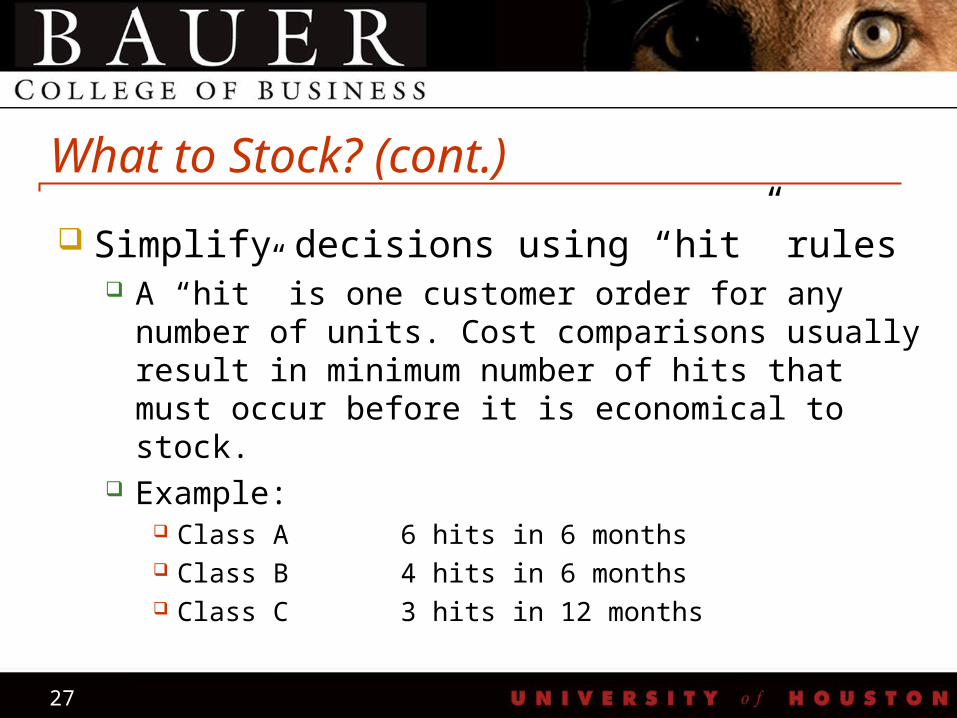
What to Stock? (cont.)

Simplify decisions using “hit” rules A “hit” is one customer order for any number of units.

Cost comparisons usually result in minimum number of hits that must occur before it is economical to stock.

Example: Class A 6 hits in 6 months Class B 4 hits in 6 months Class C 3 hits in 12 months

28

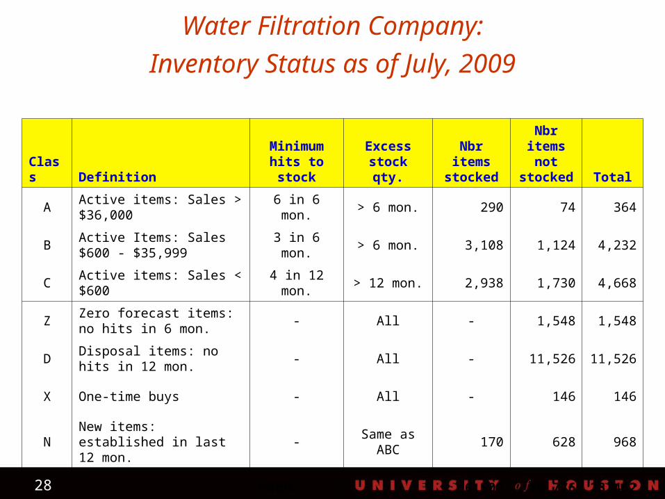
Water Filtration Company:

Inventory Status as of July, 2009

Class DefinitionMinimum

hits to stockExcess

stock qty.Nbr items stocked

Nbr items not stocked Total

AActive items: Sales > $36,000

6 in 6 mon. > 6 mon. 290 74 364

BActive Items: Sales $600 - $35,999

3 in 6 mon. > 6 mon. 3,108 1,124 4,232

C Active items: Sales < $600 4 in 12 mon. > 12 mon. 2,938 1,730 4,668

ZZero forecast items: no hits in 6 mon.

- All - 1,548 1,548

DDisposal items: no hits in 12 mon.

- All - 11,526 11,526

X One-time buys - All - 146 146

NNew items: established in last 12 mon.

-Same as

ABC170 628 968

Totals 6,506 16,776 23,452

29

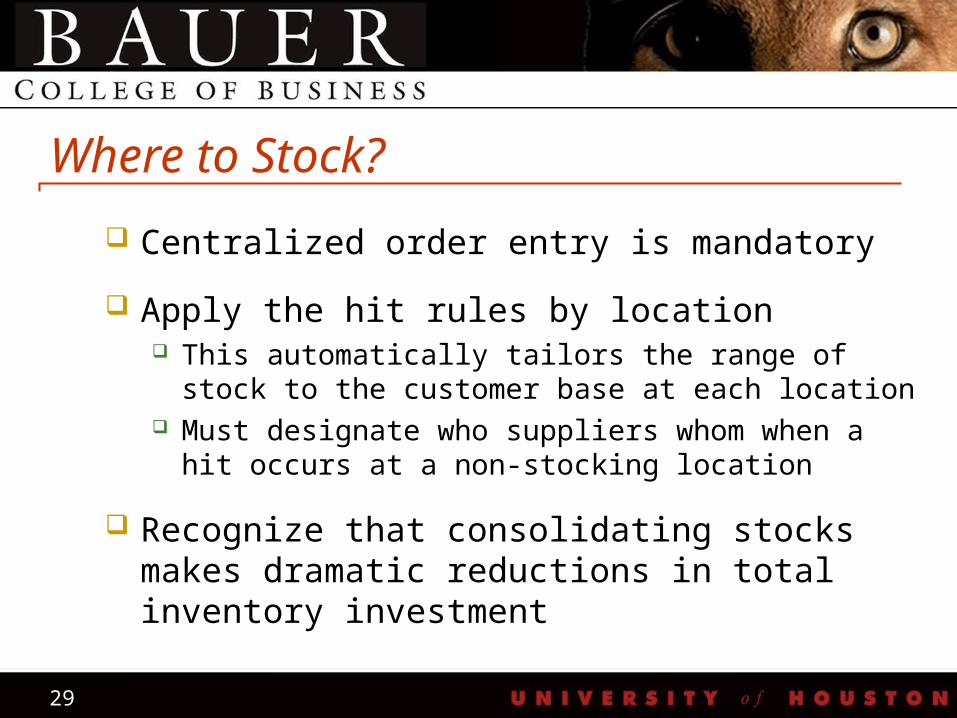
Where to Stock?

Centralized order entry is mandatory

Apply the hit rules by location This automatically tailors the range of stock to the

customer base at each location Must designate who suppliers whom when a hit occurs at

a non-stocking location

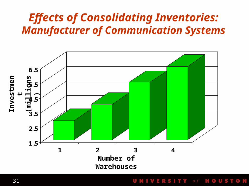
Recognize that consolidating stocks makes dramatic reductions in total inventory investment

30

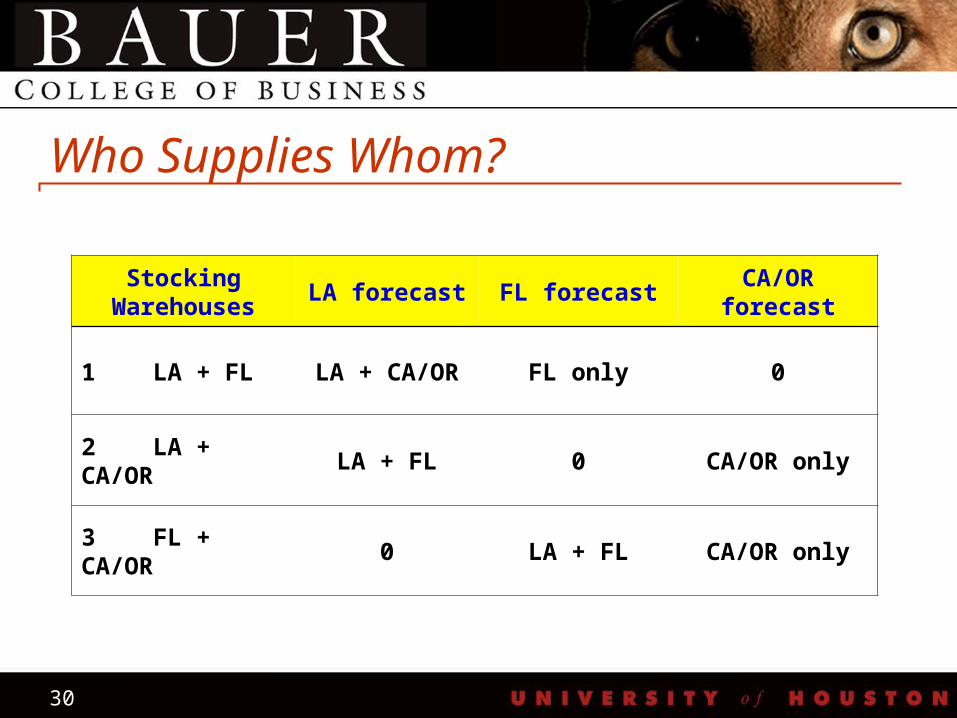
Stocking Warehouses

LA forecast FL forecast CA/OR forecast

1 LA + FL LA + CA/OR FL only 0

2 LA + CA/OR LA + FL 0 CA/OR only

3 FL + CA/OR 0 LA + FL CA/OR only

Who Supplies Whom?

31

Effects of Consolidating Inventories: Manufacturer of Communication Systems

1.5

2.5

3.5

4.5

5.5

6.5

1 2 3 4

Number of Warehouses

Inve

stm

en

t (m

illio

ns

)

32

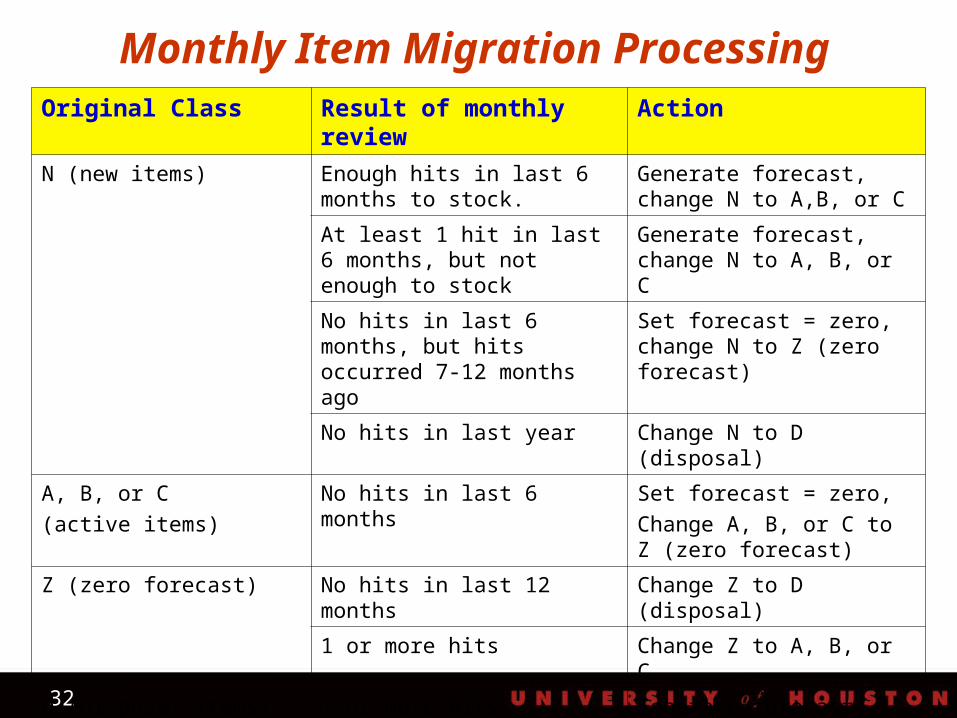
Original Class Result of monthly review Action

N (new items) Enough hits in last 6 months to stock.

Generate forecast, change N to A,B, or C

At least 1 hit in last 6 months, but not enough to stock

Generate forecast, change N to A, B, or C

No hits in last 6 months, but hits occurred 7-12 months ago

Set forecast = zero, change N to Z (zero forecast)

No hits in last year Change N to D (disposal)

A, B, or C

(active items)

No hits in last 6 months Set forecast = zero,

Change A, B, or C to Z (zero forecast)

Z (zero forecast) No hits in last 12 months Change Z to D (disposal)

1 or more hits Change Z to A, B, or C

D (disposal items) 1 or more hits Generate forecast,

Change D to A, B, or C

Monthly Item Migration Processing

33

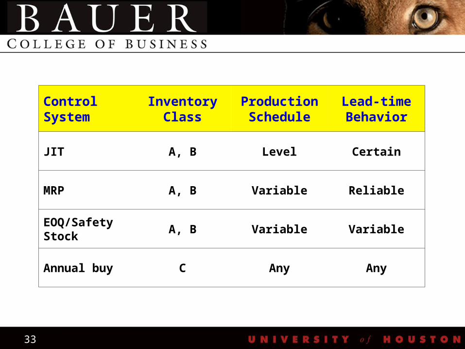
Control System

Inventory Class

Production Schedule

Lead-time Behavior

JIT A, B Level Certain

MRP A, B Variable Reliable

EOQ/Safety Stock

A, B Variable Variable

Annual buy C Any Any

34

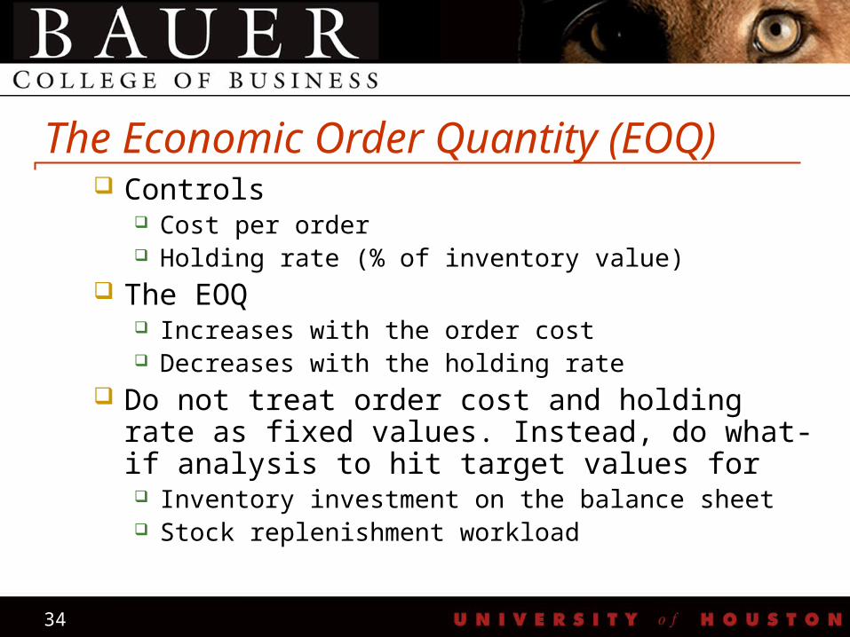
The Economic Order Quantity (EOQ) Controls

Cost per order Holding rate (% of inventory value)

The EOQ Increases with the order cost Decreases with the holding rate

Do not treat order cost and holding rate as fixed values. Instead, do what-if analysis to hit target values for Inventory investment on the balance sheet Stock replenishment workload

35

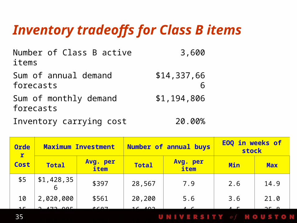
Inventory tradeoffs for Class B items

Number of Class B active items 3,600

Sum of annual demand forecasts $14,337,666

Sum of monthly demand forecasts $1,194,806

Inventory carrying cost 20.00%

Order

Cost

Maximum Investment Number of annual buysEOQ in weeks of

stock

Total Avg. per item Total Avg. per item Min Max

$5 $1,428,356 $397 28,567 7.9 2.6 14.9

10 2,020,000 $561 20,200 5.6 3.6 21.0

15 2,473,985 $687 16,493 4.6 4.5 25.8

20 2,856,711 $794 14,282 4.0 5.2 29.8

36

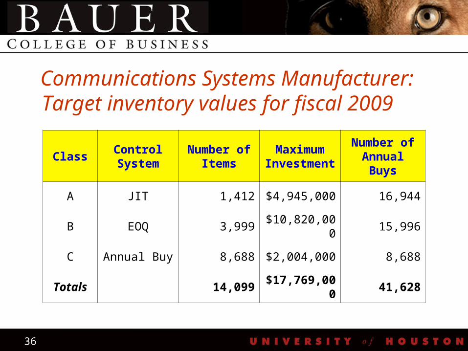
ClassControl System

Number of Items

Maximum Investment

Number of Annual Buys

A JIT 1,412 $4,945,000 16,944

B EOQ 3,999 $10,820,000 15,996

C Annual Buy 8,688 $2,004,000 8,688

Totals 14,099 $17,769,000 41,628

Communications Systems Manufacturer:Target inventory values for fiscal 2009

37

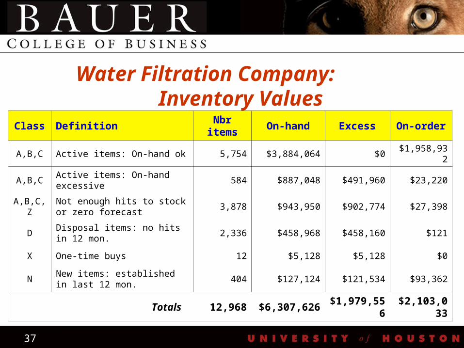
Class Definition Nbr items On-hand Excess On-order

A,B,C Active items: On-hand ok 5,754 $3,884,064 $0 $1,958,932

A,B,C Active items: On-hand excessive 584 $887,048 $491,960 $23,220

A,B,C,ZNot enough hits to stock or zero forecast

3,878 $943,950 $902,774 $27,398

DDisposal items: no hits in 12 mon.

2,336 $458,968 $458,160 $121

X One-time buys 12 $5,128 $5,128 $0

NNew items: established in last 12 mon.

404 $127,124 $121,534 $93,362

Totals 12,968 $6,307,626 $1,979,556 $2,103,033

Water Filtration Company: Inventory Values

38

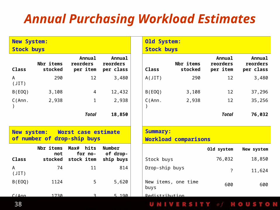
Annual Purchasing Workload Estimates

New System:

Stock buys

Old System:

Stock buys

ClassNbr items

stocked

Annual reorders per item

Annual reorders per class Class

Nbr items stocked

Annual reorders per item

Annual reorders per

class

A (JIT) 290 12 3,480 A(JIT) 290 12 3,480

B(EOQ) 3,108 4 12,432 B(EOQ) 3,108 12 37,296

C(Ann.) 2,938 1 2,938 C(Ann.) 2,938 12 35,256

Total 18,850 Total 76,032

New system: Worst case estimate of number of drop-ship buys

Summary:

Workload comparisons

ClassNbr items

not stocked

Max# hits for no-

stock item

Number of drop-

ship buys

Old system New system

Stock buys 76,032 18,850

A (JIT) 74 11 814 Drop-ship buys ? 11,624

B(EOQ) 1124 5 5,620 New items, one time buys 600 600

C(Ann.) 1730 3 5,190 Redistribution actions ? 1,600

Total 11,624 Total 76,632 32,674

39

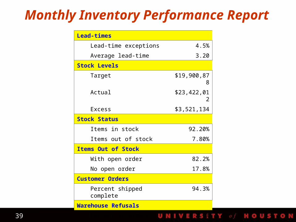
Lead-times

Lead-time exceptions 4.5%

Average lead-time 3.20

Stock Levels

Target $19,900,878

Actual $23,422,012

Excess $3,521,134

Stock Status

Items in stock 92.20%

Items out of stock 7.80%

Items Out of Stock

With open order 82.2%

No open order 17.8%

Customer Orders

Percent shipped complete 94.3%

Warehouse Refusals

Percent occurrence 2.8%

Monthly Inventory Performance Report

40

Conclusions

Forecasting drives any inventory control system

Standard ABC classification doesn’t go far enough

Decision rules for what/where to stock must be established early

41

Conclusions (cont.)

Performance measurement is essential to: Justify a new system Tailor the system to the inventory Track progress

42

Conclusions (cont.)

The best inventory system is likely to be a hybrid of: JIT MRP EOQ Annual buy