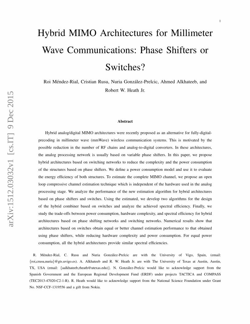
1

Hybrid MIMO Architectures for Millimeter

Wave Communications: Phase Shifters or

Switches?Roi Mendez-Rial, Cristian Rusu, Nuria Gonzalez-Prelcic, Ahmed Alkhateeb, and

Robert W. Heath Jr.

Abstract

Hybrid analog/digital MIMO architectures were recently proposed as an alternative for fully-digital-

precoding in millimeter wave (mmWave) wireless communication systems. This is motivated by the

possible reduction in the number of RF chains and analog-to-digital converters. In these architectures,

the analog processing network is usually based on variable phase shifters. In this paper, we propose

hybrid architectures based on switching networks to reduce the complexity and the power consumption

of the structures based on phase shifters. We define a power consumption model and use it to evaluate

the energy efficiency of both structures. To estimate the complete MIMO channel, we propose an open

loop compressive channel estimation technique which is independent of the hardware used in the analog

processing stage. We analyze the performance of the new estimation algorithm for hybrid architectures

based on phase shifters and switches. Using the estimated, we develop two algorithms for the design

of the hybrid combiner based on switches and analyze the achieved spectral efficiency. Finally, we

study the trade-offs between power consumption, hardware complexity, and spectral efficiency for hybrid

architectures based on phase shifting networks and switching networks. Numerical results show that

architectures based on switches obtain equal or better channel estimation performance to that obtained

using phase shifters, while reducing hardware complexity and power consumption. For equal power

consumption, all the hybrid architectures provide similar spectral efficiencies.

R. Mendez-Rial, C. Rusu and Nuria Gonzalez-Prelcic are with the University of Vigo, Spain, (email:

{roi,crusu,nuria}@gts.uvigo.es). A. Alkhateeb and R. W. Heath Jr. are with The University of Texas at Austin, Austin,

TX, USA (email: {aalkhateeb,rheath@utexas.edu)}. N. Gonzalez-Prelcic would like to acknowledge support from the

Spanish Government and the European Regional Development Fund (ERDF) under projects TACTICA and COMPASS

(TEC2013-47020-C2-1-R). R. Heath would like to acknowledge support from the National Science Foundation under Grant

No. NSF-CCF-1319556 and a gift from Nokia.

arX

iv:1

512.

0303

2v1

[cs

.IT

] 9

Dec

201

5

2

I. INTRODUCTION

Communication over millimeter wave (mmWave) frequencies will be a key feature of the fifth gen-

eration (5G) cellular networks [1]–[5]. Thanks to the large bandwidth channels potentially available,

mmWave communication can meet the high peak data rate requirements of next-generation wireless

systems. In the USA, the Federal Communication Commission has just recognized the potential of

mmWave technologies for mobile cellular in a proposed rulemaking [6]. Another potential advantage

of mmWave communication is its low latency [2], which is essential for many 5G applications, like

wearable networks [7], [8], autonomous robots, and connected or self-driving cars [9]. MmWave wireless

communication has also been considered for many other applications including local and personal area

networks [10], [11], joint vehicular communication and radar [12], [13], and simultaneous energy/data

transfer [14], [15].

One of the key architectural features of mmWave is the use of large antenna arrays at both the transmitter

and the receiver [2], [16], [17]. These arrays are used to provide array gain and obtain enough link margin

for wide area operation. Unlike lower frequency MIMO systems, the large arrays combined with high

cost and power consumption of the mixed analog/digital signal components makes it difficult to assign

an RF chain per antenna, and perform all the signal processing in the baseband [18]–[20]. This motivates

the development and analysis of new transceiver structures and their impact on MIMO signal processing

including precoding, combining, and channel estimation [21].

Analog beamforming is an approach that relies entirely on RF domain processing to reduce the number

of RF chains [22]–[24]. The beamforming is implemented using networks of analog phase shifters

that change the relative phases of the signals feeding the antennas to steer the transmit/receive beams

in the desired directions [22]–[24]. Ultimately, the performance of analog beamforming is limited by

quantization of the phase angles and the support of only single stream MIMO transmission.

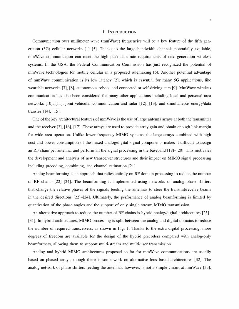
An alternative approach to reduce the number of RF chains is hybrid analog/digital architectures [25]–

[31]. In hybrid architectures, MIMO processing is split between the analog and digital domains to reduce

the number of required transceivers, as shown in Fig. 1. Thanks to the extra digital processing, more

degrees of freedom are available for the design of the hybrid precoders compared with analog-only

beamformers, allowing them to support multi-stream and multi-user transmission.

Analog and hybrid MIMO architectures proposed so far for mmWave communications are usually

based on phased arrays, though there is some work on alternative lens based architectures [32]. The

analog network of phase shifters feeding the antennas, however, is not a simple circuit at mmWave [33].

3

BasebandPrecoding

1-bitADCDAC

1-bitADCDAC

RFChain

RFChain

RF Precoding

RFChain

1-bitADCADC

1-bitADC

RFChain ADC

BasebandCombiningNt NrLt LrNs Ns

RF Combining

FBB FRF WBBWRF

Fig. 1: Hybrid MIMO architecture for mmWave communication. Precoding and combining are divided

between analog and digital domains. The number of RF chains at the transmitters/receivers are therefore

much less than the number of antennas.

Practical phased arrays use finite precision phase shifters, which may lack accuracy, and make it difficult

to finely steer the beams and place nulls. Increasing the number of bits in the phased array leads to a

higher complexity and higher power consumption. Although power consumption can be reduced using

passive phase shifters instead of active ones, the insertion losses are higher [33]. This is not desirable,

given that the combining network after the phase shifters also introduces insertion losses. Further, while

only one low-noise amplifier (LNA) per antenna is typically needed in conventional MIMO receivers,

mmWave receivers based on phased arrays require larger numbers of LNAs to achieve the same signal-

to-noise ratio (SNR) at the input of the RF chains. The effect of these practical limitations motivates the

research for alternatives to phase shifters in mmWave hybrid architectures.

In this paper, we propose new hybrid architectures based on networks of switches instead of

phase shifters in the analog processing stage. The objective of the proposed architectures is to reduce

cost, complexity, and power consumption of mmWave MIMO systems, while incurring small loss in the

system performance. We focus on the design of the combiners at the receiver, though many concepts

also extend to transmit precoding. We consider two types of switch-based hybrid architectures: (i) an

architecture where only one antenna is selected for each RF chain, and (ii) an architecture where a subset

of antennas is selected, and their outputs are combined, for each RF chain. While the first architecture

with an antenna per RF chain has lower complexity, the second one makes better use of the offered array

gain. This motivates characterizing the trade-off between the achievable rate and the power consumption

of these proposed architectures.

To compare the different switch-based and phase shifter-based hybrid architectures, we develop a

power consumption model for mmWave MIMO receivers. The developed model provides a general

framework for calculating the consumed power in the hybrid architectures as a function of the numbers

4

of antennas and RF chains. Using this model and approximated power consumption numbers from recent

RF circuit designs [33]–[60], we show that switches based architectures can yield reasonable reduction

in the power consumption, especially with large antenna arrays.

To exploit the new proposed architectures, we develop new mmWave channel estimation algorithms

to configure the hybrid precoders and combiners. Channel estimation is difficult in mmWave because of

the large channel dimensions and the low receive SNR before beamforming design [20]. With hybrid

architectures, the mmWave channel estimation problem becomes more difficult and architecture-dependent

because the channel is seen at the baseband through the RF lens. Exploiting channel sparsity, though,

channel estimation at mmWave can be formulated as a compressive channel estimation problem [61],

where different compressed sensing (CS) tools can be leveraged to estimate the channels [29], [62]–[65].

Compressive estimation of sparse spatial channels at mmWave was first proposed in [62] for an analog

beamforming architecture. The algorithm estimates a predetermined number of paths using a coarse grid

for the possible spatial frequencies, then refines those estimates using Newton’s method. In [29] a hybrid

architecture is considered, and adaptive compressed sensing tools from [66] were leveraged to iteratively

estimate the dominant paths of mmWave channels. In [63], [64], compressed sensing with random training

sequences were adopted also for channel estimation in hybrid architectures. An extension to multi-user

mmWave systems was provided in [65], where multiple users estimate their channels simultaneously.

The solutions in [29], [63]–[65] all focus on mmWave channel estimation and the training signals design

assuming phase shifters are used for the analog beamforming stage. They cannot be used for switches.

We propose an open loop strategy for downlink mmWave channel estimation. The proposed

algorithm is independent of the hardware used in the analog processing stage and thus can be applied to

either phase shifter or switching networks. It also incorporates hybrid constraints at both the transmitter

and receiver during training, and leverages mmWave channel sparsity in the angular domain. For each

of the proposed architectures, we design efficient training beamformers and combiners that lead to

appropriate CS measurement matrices, and derive bounds on their performance. For the noiseless case, we

find the optimal number of training measurements that minimizes the Welch bound on the coherence of the

equivalent measurement matrix [67]. Using the normalized mean squared error (NMSE) as a performance

metric, we show by simulations that the developed training sequence designs and channel estimation

algorithms with switch-based architectures can achieve comparable performance to that obtained with

phase shifter based architectures, while requiring lower power consumption.

Given an estimate of the channel, it is possible to optimally configure the hybrid precoders and

combiners. In [25], hybrid precoders were designed in general MIMO systems for multiplexing gain

5

maximization; interference management was further incorporated in [26]. Leveraging mmWave channel

sparsity, [27] developed an orthogonal matching pursuit based solution for hybrid precoders in mmWave

systems, assuming perfect channel knowledge. Designs that do not rely on matching pursuit have been

proposed in [68], [69]. The solutions in [27], [68], [69], though, considered hybrid architectures with ana-

log phase shifters. For the switch-based hybrid architectures, the design of the analog precoders/combiners

is related to the antenna (subset) selection problem, which is a classical topic in the MIMO literature (see

e.g. [70], [71] and the references therein). Prior work on antenna subset selection, however, focused on

fully-digital and not hybrid switch-based architectures. Therefore, new precoding/combining algorithms

need to be developed for the proposed switch-based hybrid architectures.

In this paper, we devise adaptive strategies for the design of the switch-based hybrid architectures

with antenna subset selection. The proposed solutions incorporate hybrid constraints into the greedy

algorithms in [72]. Equipped with a channel estimator and a means of deriving the precoding and

combining matrices, we analyze the performance of the different architectures in numerical simulations.

We compare the achieved spectral efficiencies of the proposed switch-based hybrid precoding/combining

algorithms with that obtained using fully-digital architectures and phase-shifters hybrid analog/digital

constraints. From these results, we conclude that architectures based on switches can achieve similar

spectral efficiencies for equal power consumption. Further, when comparing all architectures operating

with the same number of RF chains, we find that those architectures based on switches require lower

power consumption at the cost of a small loss in the array gain, which slightly impacts the obtained

spectral efficiency.

In summary, we provide a complete design of several hybrid mmWave architectures based on switching

networks for the analog processing stage. In Section II, we define the system model and describe four

different MIMO architectures that make use of antenna switches and subarrays. Then we develop a

power consumption model in Section III, and use it to craft a comparison between the power efficiency

of the different proposed architectures. We present the design of a novel compressive channel estimator in

Section IV, which can be used with either phase shifters or switches in the analog processing. Based on

the channel estimates, we propose algorithms for the design of the analog and digital combining matrices

in Section V. Then in Section VI we compare the different architectures in terms of channel estimation

error and spectral efficiency, showing when the switch-based architecture is preferred. We make some

concluding remarks in Section VII.

We use the following notation throughout this paper: bold lowercase a is used to denote column

vectors, bold uppercase A is used to denote matrices, non-bold letters a,A are used to denote scalar

6

values, and caligraphic letters A to denote sets. Using this notation, |a| is the magnitude of a scalar,

‖a‖2 is the `2 norm, ‖a‖0 is the `0 pseudo-norm, ‖A‖F is the Frobenius norm, σk(A) denotes the kth

singular value of A in decreasing order, tr(A) denotes the trace, A∗ is the conjugate transpose, AT is

the matrix transpose, A−1 denotes the inverse of a square matrix, ak is the kth entry of a, |A| is the

cardinality of set A. A ⊗ B is the Kronecker product of A and B. We use the notation N (m,R) to

denote a complex circularly symmetric Gaussian random vector with mean m and covariance R. We use

E to denote expectation.

II. SYSTEM MODEL

Consider the single-user mmWave hybrid MIMO system in Fig. 1. In this paper we focus on the

downlink and specifically consider antenna selection at the mobile station (MS) where the complexity and

power consumption limitations are especially important. While we describe the general model including

hybrid operation at both the BS and the MS, we focus on the combining operation at the MS since the

base station typically has less restrictive power constraints.

The transmitting BS is equipped with Nt antennas and Lt RF chains, while the receiving MS has Nr

antennas and Lr RF chains. Ns data streams are transmitted from the BS to the MS assuming Ns ≤ Lt ≤

Nt and Ns ≤ Lr ≤ Nr. The transmitter applies a hybrid precoder F to the symbol vector s ∈ CNs×1 with

E[ss∗] = 1Ns

I. The hybrid precoder F = FRFFBB is composed of an RF precoder FRF ∈ CNt×Lt , and a

baseband digital precoder FBB ∈ CLt×Ns . The discrete-time transmitted signal is given by x = Fs.

We consider a narrowband frequency-flat channel model represented by the channel matrix H ∈

CNr×Nt , with E[‖H‖2F

]= NtNr. Assuming perfect synchronization, the received signal can be written

as

r =√ρHFs + n, (1)

where ρ represents the average received power and n ∈ CNr×1 is the noise vector with CN (0, σ2n) entries.

The MS applies a hybrid combiner W to the received signal so that the processed received signal is

y =√ρW∗HFs + W∗n. (2)

The hybrid combiner W = WRFWBB is composed of an RF combiner WRF ∈ CNr×Lr and a

baseband combiner WBB ∈ CLr×Ns . The RF precoder and combiner are implemented in analog, so

that the precoding and combining matrices FRF and WRF are subject to specific constraints depending

on the hardware used to implement the analog precoder/combiner.

7

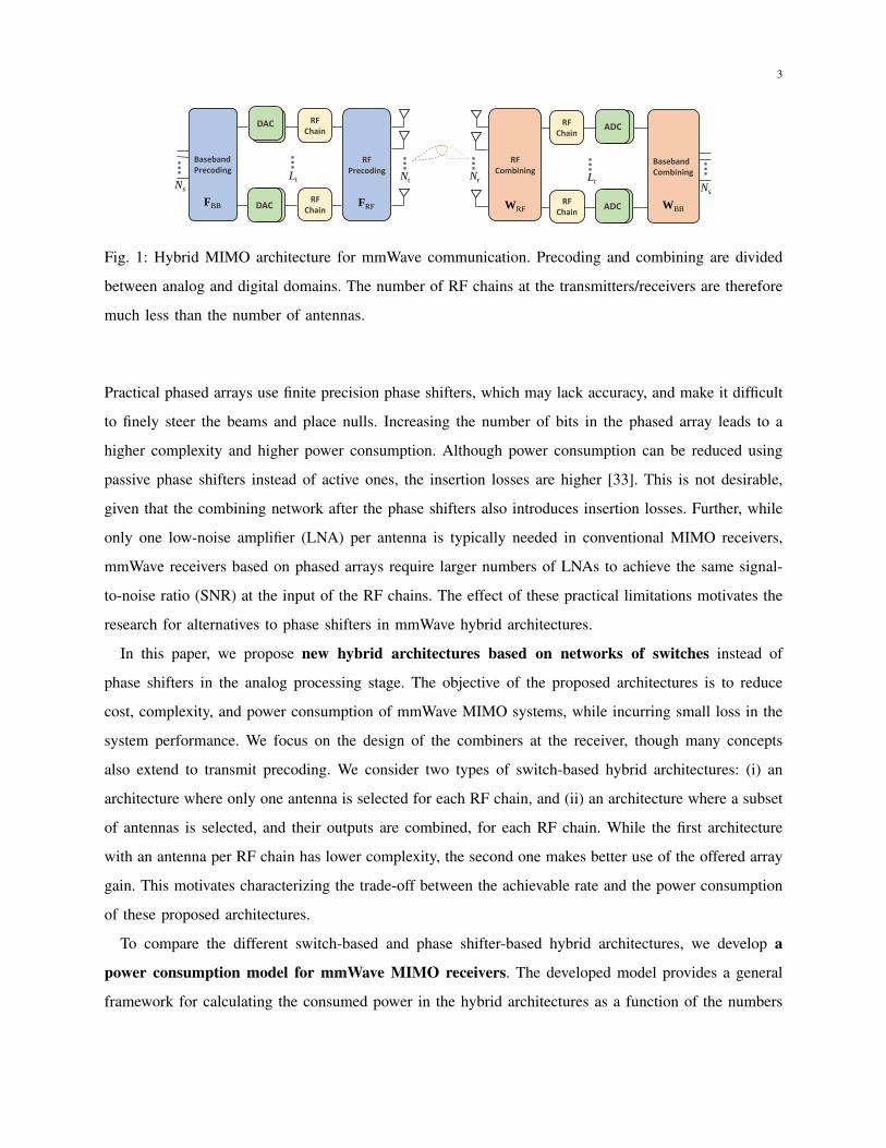
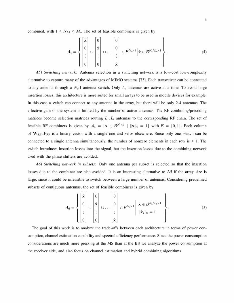
We consider two hybrid architectures that use phase shifters based on previous work. Further, we

propose four new hybrid precoding architectures based on switches. Fig. 2 shows the block diagrams

corresponding to all these architectures, which are further explained in the following.

A1) Phase shifting network: Each transceiver is connected to each antenna through a network of

phase shifters. Assuming infinite resolution phase shifters, the incoming signals are combined before

feeding the RF chain. Each transceiver achieves full array gain emulating an antenna with high aperture.

An RF precoder/combiner implemented with a network of variable phase shifters imposes the constraint

of unit norm entries in WRF and FRF. The set of feasible combining vectors, e.g. columns of WRF, is

given by A1 = {x ∈ CNr×1 | |xi| = 1}.

A2) Phase shifting network in subsets: Each transceiver is routed to a subset of Mr = Nr/Lr

antennas through an analog preprocessing network of analog phase shifters. This is essentially an array-

of-subarrays hybrid architectures, which assume that each RF is connected to a unique subset of the

antennas [30], [31]. Compared to architecture A1, the maximum gain of each transceiver is reduced by

a factor 1/Lr. The complexity of this architecture, however, is lower and it requires only Nr RF paths

and analog phase shifters instead of the Nr × Lr needed in A1. This solution is interesting for the BS

in multiuser scenarios, since the antenna grouping reduces the mutual coupling and interference between

users [30]. The set of feasible RF combining vectors is given by

A2 =

x

0

...

0

∪

0

x

...

0

∪ . . .

0

0

...

x

∈ CNr×1

∣∣∣∣∣∣ x ∈ CNr/Lr×1

|xi| = 1

. (3)

A3) Switching network with analog combining: In this new architecture, each transceiver is routed

to each antenna through an network of switches. A3 is equivalent to A1, replacing each variable phase

shifter by a simple switch. Each transceiver selects a subset of NA3 antennas, between 1 and Nr, whose

received signal will be non coherently combined before feeding the RF chain, which could result in a

degradation of the SNR. Therefore, designing an optimal combiner presents challenging issues. The set

of feasible RF combiners is given by A3 = {x ∈ BNr×1}, where B is the binary set {0, 1}.

A4) Switching network in subsets with analog combining: In this case each antenna is routed to a

single switch, avoiding the need of splitters and the following LNAs, which results in a lower power

consumption than the previous architecture. Only NA4 of the antennas in every subset of size Mr are

8

combined, with 1 ≤ NA4 ≤Mr. The set of feasible combiners is given by

A4 =

x

0

...

0

∪

0

x

...

0

∪ . . .

0

0

...

x

∈ BNr×1

∣∣∣x ∈ BNr/Lr×1

. (4)

A5) Switching network: Antenna selection in a switching network is a low-cost low-complexity

alternative to capture many of the advantages of MIMO systems [73]. Each transceiver can be connected

to any antenna through a Nr:1 antenna switch. Only Lr antennas are active at a time. To avoid large

insertion losses, this architecture is more suited for small arrays to be used in mobile devices for example.

In this case a switch can connect to any antenna in the array, but there will be only 2-4 antennas. The

effective gain of the system is limited by the number of active antennas. The RF combining/precoding

matrices become selection matrices routing Lr, Lt antennas to the corresponding RF chain. The set of

feasible RF combiners is given by A5 = {x ∈ BNr×1 | ‖x‖0 = 1} with B = {0, 1}. Each column

of WRF,FRF is a binary vector with a single one and zeros elsewhere. Since only one switch can be

connected to a single antenna simultaneously, the number of nonzero elements in each row is ≤ 1. The

switch introduces insertion losses into the signal, but the insertion losses due to the combining network

used with the phase shifters are avoided.

A6) Switching network in subsets: Only one antenna per subset is selected so that the insertion

losses due to the combiner are also avoided. It is an interesting alternative to A5 if the array size is

large, since it could be infeasible to switch between a large number of antennas. Considering predefined

subsets of contiguous antennas, the set of feasible combiners is given by

A6 =

x

0

...

0

∪

0

x

...

0

∪ . . .

0

0

...

x

∈ BNr×1

∣∣∣∣∣∣ x ∈ BNr/Lr×1

‖xi‖0 = 1

. (5)

The goal of this work is to analyze the trade-offs between each architecture in terms of power con-

sumption, channel estimation capability and spectral efficiency performance. Since the power consumption

considerations are much more pressing at the MS than at the BS we analyze the power consumption at

the receiver side, and also focus on channel estimation and hybrid combining algorithms.

9

(a) A1: Architecture with variable phase shifters (b) A2: Architecture with variable

phase shifters in subsets of antennas

(c) A3: Antenna selection with analog com-

bining

(d) A4: Antenna selection in subsets

with analog combining

(e) A5: Antenna selection (f) A6: Antenna selection in

subsets

Fig. 2: Analog architectures for the RF combiner.

10

III. POWER CONSUMPTION MODEL

Understanding power consumption is important for characterizing tradeoffs between the different hybrid

architectures. In this section, we develop an approximate power consumption model for the architectures

in Fig. 2. Our aim is to compare the architectures proposed in the previous section in terms of power

consumption for different values of the array size and the number of RF chains. Since exact computation

of the dissipated power is difficult in general, we approximate the power consumption of each hardware

component and give reasonable arguments for the choice we make. We focus the analysis only on the

receiver side. A similar model can be derived for the transmitter replacing the low noise amplifiers (LNA)

by power amplifiers (PA), and the ADCs with DACs.

We denote as PLNA the power consumed by a single LNA and PADC the power consumed by a single

ADC. We assume that all the architectures use the same kind of ADCs and LNAs. Recent work on the

development of low power LNAs for the 60 GHz band in CMOS technology [34]–[37], show that power

consumption for an LNA at 60 GHz is in the range of 4.6 to 86 mW. Other results in the literature, for

example the mmWave picocellular system in [38], estimated the LNA consumption at 20 mW which is

within our range. In this paper we will assume PLNA = 20 mW.

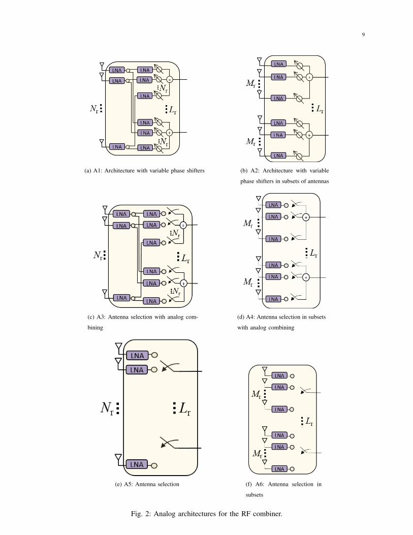
Regarding power consumption of mmWave ADCs, we focus on devices that can be used in a 60

GHz system with at least a 500 MHz bandwidth and an effective resolution (ENOB) larger than 4 bits.

Table I shows ADC power consumption versus maximum sampling frequency and effective number of bits

(ENOB) for different designs proposed between 2012 and 2015. The values show the power consumption

of prototype ADCs that can be found in the recent scientific literature. Although they give a clear trend in

the development of low power ADCs, to be conservative about the power consumption of commercially

available mmWave converters in the future years, we consider a reference value of PADC = 200 mW, that

includes the conversion of the I and Q components (note that some of the integrated designs referenced in

the table already include two converters). The choice of the reference value is difficult in this case since

the values in Table I present high variability and therefore a threshold cannot be clearly discerned. We

choose a conservative (high) value since the designs in Table I are not commercial products and as such we

might expect these values to be relatively optimistic (low), as compared to the power consumption of the

final working devices. Furthermore, previous work [38] in the same context of mmWave communications

also considers a similar reference value.

RF phase shifters are key components in integrated mmWave phased arrays. Some important con-

siderations regarding the phase shifter design are the noise figure, power consumption, insertion loss,

11

Maximum Power

Reference Year sampling ENOBhf consumption

rate

[Gs/s] [bits] [mW]

Hong et al. [39] 2015 1.7 8.21 15.4

Sung et al. [40] 2015 1.6 9 17.3

Le Dortz et al. [41] 2014 1.62 7.68 93

Dong et al. [42] 2014 3.20 11.77 240

Lee et al. [43] 2014 1.0 8.2 19.8

Miyahara et al. [44] 2014 2.2 5.92 27

Janssen et al. [45] 2013 3.6 8.01 795

Kull et al. [46] 2013 1.2 6.24 3.1

Tabasy et al. [47] 2013 3 4.56 79.1

Shettigar et al. [48] 2012 3.6 11.49 15

TABLE I: ADC power consumption versus sampling frequency and effective number of bits.

loss variation over the range of shift, linearity, resolution and bandwidth. Phase shifters at mmWave

frequencies can be classified into: (i) active phase shifters, such as reflective, loaded line, switched delay;

and (ii) passive phase phase shifters, such as cartesian vector modulator, LO-path phase shifter, and phase-

oversampling vector modulator [33] [49]. Active phase shifters have a small footprint but generally cause

nonlinearity problems resulting in a high noise figure. Passive phase shifters occupy a larger area and

incur in large insertion losses. Although there is not a significant noise trade-off between active and

passive phase shifters [50], the power consumption with passive phase shifters is lower, which make

them preferable for applications requiring mobility and autonomy. The main challenge associated with

passive phase shifters is the dependency of the insertion losses on the phase shift setting. To compensate

this effect, variable gain amplifiers (VGAs) with integrated phase-compensated technique are usually

added following the passive phase shifter [50].

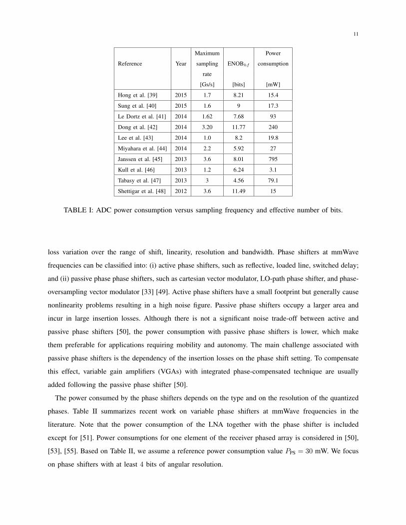
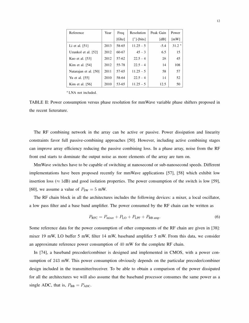
The power consumed by the phase shifters depends on the type and on the resolution of the quantized

phases. Table II summarizes recent work on variable phase shifters at mmWave frequencies in the

literature. Note that the power consumption of the LNA together with the phase shifter is included

except for [51]. Power consumptions for one element of the receiver phased array is considered in [50],

[53], [55]. Based on Table II, we assume a reference power consumption value PPS = 30 mW. We focus

on phase shifters with at least 4 bits of angular resolution.

12

Reference Year Freq Resolution Peak Gain Power

[Ghz] [◦]-[bits] [dB] [mW]

Li et al. [51] 2013 58-65 11.25 - 5 -5.4 31.2 a

Uzunkol et al. [52] 2012 60-67 45 - 3 6.5 15

Kuo et al. [53] 2012 57-62 22.5 - 4 28 45

Kim et al. [54] 2012 55-78 22.5 - 4 14 108

Natarajan et al. [50] 2011 57-65 11.25 - 5 58 57

Yu et al. [55] 2010 58-64 22.5 - 4 14 52

Kim et al. [56] 2010 53-65 11.25 - 5 12.5 50

a LNA not included.

TABLE II: Power consumption versus phase resolution for mmWave variable phase shifters proposed in

the recent lieterature.

The RF combining network in the array can be active or passive. Power dissipation and linearity

constraints favor full passive-combining approaches [50]. However, including active combining stages

can improve array efficiency reducing the passive combining loss. In a phase array, noise from the RF

front end starts to dominate the output noise as more elements of the array are turn on.

MmWave switches have to be capable of switching at nanosecond or sub-nanosecond speeds. Different

implementations have been proposed recently for mmWave applications [57], [58] which exhibit low

insertion loss (≈ 1dB) and good isolation properties. The power consumption of the switch is low [59],

[60], we assume a value of PSW = 5 mW.

The RF chain block in all the architectures includes the following devices: a mixer, a local oscillator,

a low pass filter and a base band amplifier. The power consumed by the RF chain can be written as

PRFC = Pmixer + PLO + PLPF + PBB amp. (6)

Some reference data for the power consumption of other components of the RF chain are given in [38]:

mixer 19 mW, LO buffer 5 mW, filter 14 mW, baseband amplifier 5 mW. From this data, we consider

an approximate reference power consumption of 40 mW for the complete RF chain.

In [74], a baseband precoder/combiner is designed and implemented in CMOS, with a power con-

sumption of 243 mW. This power consumption obviously depends on the particular precoder/combiner

design included in the transmitter/receiver. To be able to obtain a comparison of the power dissipated

for all the architectures we will also assume that the baseband processor consumes the same power as a

single ADC, that is, PBB = PADC.

13

Based on the block diagrams, the power dissipated by the hybrid combining architectures can be written

respectively as

PA1 = Nr(Lr + 1)PLNA +NrLrPPS + Lr(PRFC + PADC) (7)

+ PBB (8)

PA2 = NrPLNA +NrPPS + Lr(PRFC + PADC) + PBB, (9)

PA3 = (Nr + LrNA3)PLNA + LrNA3PSW (10)

+ Lr(PRFC + PADC) + PBB, (11)

PA4 = LrNA4(PLNA + PSW) + Lr(PRFC + PADC) + PBB, (12)

PA5 = Lr(PLNA + PSW) + Lr(PRFC + PADC) + PBB, (13)

PA6 = Lr(PLNA + PSW) + Lr(PRFC + PADC) + PBB, (14)

Note that the power consumption for the architecture (A2) does not depend on the array size, but on

the number of RF chains. The power consumption of a complete antenna array with one RF chain per

antenna is

PD = Nr(PLNA + PRFC + PADC) + PBB. (15)

The percentage of power consumption reduction that can be achieved with the hybrid architectures respect

to that of the complete system can be written as

ηi = Pi/PD, i = 1 . . . 4. (16)

To compare power consumption we write these equations in terms of a single power value Pref = 20

mW. In this way:

PLNA = Pref

PADC = 10Pref

PRF chain = 2Pref

PBB = 10Pref

PPS = 1.5Pref

PSW = 0.25Pref

14

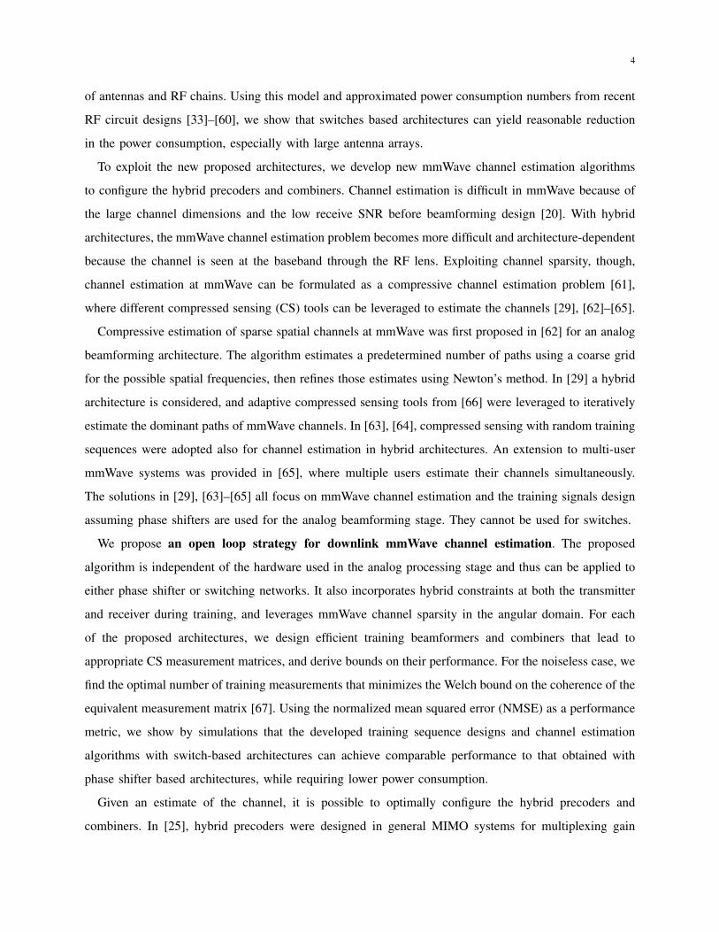
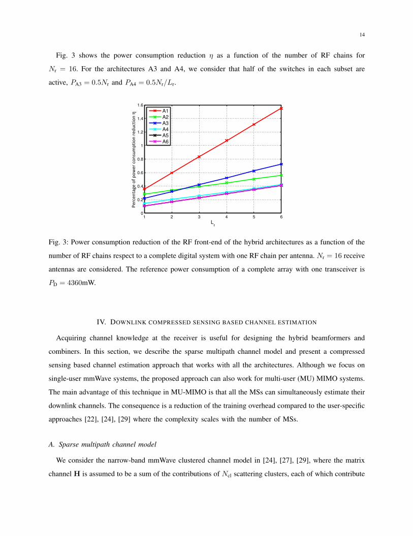
Fig. 3 shows the power consumption reduction η as a function of the number of RF chains for

Nr = 16. For the architectures A3 and A4, we consider that half of the switches in each subset are

active, PA3 = 0.5Nr and PA4 = 0.5Nr/Lr.

1 2 3 4 5 60

0.2

0.4

0.6

0.8

1

1.2

1.4

1.6

Lr

Perc

enta

ge o

f pow

er c

onsu

mpt

ion

redu

ctio

n η

A1

A2

A3

A4

A5

A6

Fig. 3: Power consumption reduction of the RF front-end of the hybrid architectures as a function of the

number of RF chains respect to a complete digital system with one RF chain per antenna. Nr = 16 receive

antennas are considered. The reference power consumption of a complete array with one transceiver is

PD = 4360mW.

IV. DOWNLINK COMPRESSED SENSING BASED CHANNEL ESTIMATION

Acquiring channel knowledge at the receiver is useful for designing the hybrid beamformers and

combiners. In this section, we describe the sparse multipath channel model and present a compressed

sensing based channel estimation approach that works with all the architectures. Although we focus on

single-user mmWave systems, the proposed approach can also work for multi-user (MU) MIMO systems.

The main advantage of this technique in MU-MIMO is that all the MSs can simultaneously estimate their

downlink channels. The consequence is a reduction of the training overhead compared to the user-specific

approaches [22], [24], [29] where the complexity scales with the number of MSs.

A. Sparse multipath channel model

We consider the narrow-band mmWave clustered channel model in [24], [27], [29], where the matrix

channel H is assumed to be a sum of the contributions of Ncl scattering clusters, each of which contribute

15

Nray propagation paths. The physical channel model H ∈ CNr×Nt can be expressed as

H =

√NtNr

NclNray

Ncl∑i=1

Nray∑`=1

βi,`aMS(φi,`)a∗BS(αi,`), (17)

where βi,` is the complex gain of the `th ray in the ith cluster, whereas aBS(αi,`) and aMS(φi,`) are the

antenna array response vectors at the transmitter and receiver evaluated at the `th path ith cluster azimuth

angles of departure or arrival. The multipath channel model (17) can be written in a more compact way

as

H = AMSHbA∗MS, (18)

where AMS ∈ CNr×NclNray and ABS ∈ CNt×NclNray contain the array response vectors in the directions φi,`

and αi,`, and Hb is a diagonal matrix with the associated path gains βi,`. MmWave channels are expected

to have limited scattering [75], therefore, a small number of propagation paths K = NclNray is assumed.

The highly directional nature of propagation and the high dimensionality of MIMO channels at

mmWave frequencies makes the beamspace representation of MIMO systems a natural choice [20].

Assuming that the AoAs and AoDs φ, α are taken from uniform fine grids of Gr and Gt points in [−π2 ,

π2 ),

we define two dictionary matrices AMSD = [aMS(φ1) . . .aMS(φGr)] and ABSD = [aBS(α1) . . .aBS(αGr)],

with the associated array response vector in these directions. Neglecting the grid quantization error, we

can represent H in terms of a K-sparse matrix Hv ∈ CGr×Gr containing the path gains of the quantized

angles

H = AMSDHvA∗BSD. (19)

This representation provides a discretized approximation of the channel response that reduces the task

of estimating H to that of detecting some non zero coefficients in the virtual channel matrix Hv [61].

Vectorizing the channel matrix we have

vec(H) = (ABSD ⊗AMSD)x, (20)

where x = vec(Hv) is a GtGr × 1 sparse vector with K non zero entries. We define the NtNr × GtGr

dictionary matrix of the channel Ψ = (ABSD⊗AMSD). Each column of Ψ is of the form aBS(α)⊗aMS(φ).

Assuming uniform spaced linear arrays with inter-element spacing equal to half wavelength, λ/2, and

the quantized AoAs and AoDs are taken from uniform fine grids of resolution Gr = Nr and Gt = Nt

points, the array response matrices result in unitary DFT matrices AMSD ∈ CNr×Nr and ABSD ∈ CNt×Nt .

This case is known as the virtual channel model [76], which corresponds to beamforming in fixed

directions determined by the resolution of the arrays.

16

B. Compressed channel sensing

In this section we present a training-based channel estimation approach. The mmWave channel esti-

mation is formulated as a sparse reconstruction problem [77], [78]. The BS and MS sense the channel

in open loop with a sequence of training precoders and combiners. The reconstruction is done applying

a standard greedy recovery algorithm.

Consider the mmWave system and channel model described in the previous section. Let us assume

first that the BS and MS employ only one RF chain for the training step. At time instant n, the BS uses a

training beamformer pn to transmit a symbol sn. To simplify the analysis we consider the same symbol

s = 1 in all the transmissions. The MS applies a training combiner vector qn to the received signal.

Then the resulting signal can be written as [29]

yn =√ρq∗nHpns+ q∗nn (21)

=√ρ(pTn ⊗ q∗n)vec(H) + q∗nn (22)

=√ρ(pTn ⊗ q∗n)Ψx + q∗nn. (23)

The BS employs M precoding vectors [p1, . . . ,pM ] and the MS employs M combiners [q1, . . . ,qM ] in

successive M snapshots. Stacking the M measurements in vector form we have

y1...

yM

=√ρ

pT1 ⊗ q∗1

pT2 ⊗ q∗2...

pTM ⊗ q∗M ,

Ψx + e. (24)

Assuming q∗iqi = γ due to hardware constraints, the combined noise vector is given by e = [q∗1n1, . . . ,q∗MnM ]T

with covariance E[ee∗] = σ2nγIM .

The generalization of the approach to many RF chains is as follows. The BS employs a sequence of Mt

beamforming vectors P = [p1, . . . ,pMt ] in successive Mt time instants. If the MS utilizes the available

Lr RF chains, it can apply simultaneously Lr combiners Qn = [qn1 , . . . ,qnLr

] ∈ CNr×Lr per snapshot to

the received signal. In this way, Lr channel measurements are produced per time instant. The sequence

of training combiners is defined as Q = [Q1, . . . ,QMt ] ∈ CNr×MtLr . After Mt snapshots and stacking

17

the M = MtLr measurements in vector form we havey1...

yM

=√ρ

pT1 ⊗Q∗1

pT2 ⊗Q∗2...

pTMt⊗Q∗Mt

Ψx + e. (25)

The noise vector is given by e = [Q∗1n1 . . .Q∗Mt

nMt ]T , with block diagonal covariance matrix E[ee∗] =

σ2ndiag(Q∗1Q1, . . . ,Q∗Mt

QMt). In general the noise is correlated after combining, except for A5, where

Q∗iQi = ILr and the noise remains uncorrelated.

Notice that the number of compressed measurements per snapshot depends on the number of available

RF chains at the MS but not on the number of RF chains at the BS, since the receive signals are combined

at the MS. The higher the number of RF chains used simultaneously in reception, the higher the number

of measurements per snapshot.

C. Channel reconstruction and recovery guarantees

Since mmWave channels exhibit a sparse-scattering structure, it is possible to leverage theory and

algorithms developed for sparse recovery to improve channel estimation results.

Equations (24) and (25) can be seen as a single measurement vector (SMV) compressive sensing

model with the unknown x, a K-sparse vector. Estimating the support of x is equivalent to estimating the

direction of the AoA and AoD of the channel paths, while the values of these non-zero entries correspond

to the path gains. The reconstruction of the channel is formulated as a non-convex combinatorial problem

minimizex

‖x‖0 subject to ‖y −Ax‖2 ≤ σ, (26)

where the matrix A = ΦΨ ∈ CM×N , with N = GrGt. A variety of Matching Pursuit (MP) algorithms

have been proposed for obtaining an approximate solution in polynomial complexity. We consider Or-

thogonal Matching Pursuit (OMP) for its simplicity and fast implementation. OMP has been used for

compressed sensing channel estimation [79].

The problem of recovering a high-dimensional sparse signal based on a small number of linear

measurements, possibly corrupted by noise, has been extensively studied in compressed sensing. Recovery

guarantees can be obtained providing that the matrix A has low coherence. The mutual coherence of

a given matrix A is the largest absolute normalized inner product between different columns from A.

Suppose A = [a1 a2 ... aN ], the mutual coherence of A is given by

µ(A) = maxk,j; k 6=j

|a∗kaj |‖ak‖2‖aj‖2

. (27)

18

OMP support recovery guarantee has been stated in the noiseless case in [80]. It was shown that µ(A) <

12K−1 is a sufficient condition for recovering a K-sparse x exactly in the noiseless case. This condition

is in fact sharp [81]. In [67], the lower bound of the achievable coherence of a matrix A of size M ×N ,

with M ≤ N , is given by the Welch bound

µ(A) ≥

√N −MM(N − 1)

. (28)

For a given coherence µ(A), it is possible perfectly to recover a K-sparse vector provided K <(µ(A)−1 + 1

)/2. Therefore, in the noiseless case, the minimum number of measurements M needed to

guarantee the recovery of K-sparse vectors is given by√N −MM(N − 1)

<1

2K − 1. (29)

The OMP recovery guarantees in the presence of noise were considered in [82]. They require the noise

power to be lower than the norm of the non-zero entries in the unknown x. This means that we can

guarantee that OMP will perform well if the SNR is not too low.

Alternatively, recovery guarantees are provided if A satisfies the restricted isometry property (RIP). A

matrix A ∈ CM×N is said to posses the RIP with isometry constant δ if

(1− δ)‖x‖22 ≤ ‖Ax‖22 ≤ (1 + δ)‖x‖22 for all K-sparse x, (30)

and δ is small enough for sufficiently large K. The RIP guarantees uniform recovery of K-sparse vectors

and moreover the reconstructions (by various approximation algorithms) are stable even when sparsity

is replaced by compressibility and it is robust in the presence of noise. Several classes of matrices that

obey RIP, like Gaussian and Rademacher/Bernoulli, are easy to construct [83], [84].

At low SNR, the number of measurement M needs to increase to ensure the quality of the estimate.

In fact, the number of measurements is very sensitive to the sparsity of the virtual channel matrix and

the SNR. When the sparsity is low, only a few measurements (M � N ) are needed for good recovery

as predicted by the CS theory [83]. When the SNR is very low or the sparsity is high, the number of

measurement needed is comparable or even higher than the dimension of x.

There are several stopping criteria for OMP that can be implemented with minimal cost. A natural way

is to stop the algorithm when the sparsity order is reached. Usually the sparsity order is itself subject

to estimation and may not be available. Therefore, stopping criteria based on the power of the residual

error are often used. Let rk the residual error at iteration k, we stop the algorithm when the energy in

the residual is smaller than a given threshold ‖rk‖2 ≤ ε. A reasonable choice for the stopping threshold

is ε = E[e∗e], the noise power after combining. This is the choice made in this manuscript.

19

D. Training sequences and mutual coherence

The matrix A = ΦΨ plays a key role in establishing recovery guarantees for the compressed sensing

channel estimation problem. In this section we design training sequences of precoding/combining vectors

that define the sensing matrix Φ and provide low coherence. Φ is hardware dependent, therefore, we

have to take into account the restrictions imposed by the specific architecture. For instance, the phase

shifter architecture A1 constrains the precoding/combining vectors p, and q to have unit norm entries,

while a switching architecture A5 constrains the combining/precoding vectors to have exactly a one and

zeros elsewhere. In this paper we describe two ways of constructing the sensing matrix, one using the

same combiner sequence for all precoders and another using different combiners for each precoder.

1) Single combiner matrix (SC): We start the analysis considering a more restrictive structure of the

sensing matrix. Consider that the MS applies a fixed sequence of combiners Q = [q1, . . . ,qMr ] ∈ CNr×Mr

for each precoding vector in P = [p1, . . . ,pMt ] ∈ CNt×Mt

Φ =

pT1 ⊗Q∗

pT2 ⊗Q∗

...

pTMt⊗Q∗

, (31)

which can be written in a compact way as Φ = (PT ⊗Q∗) ∈ CM×NtNr , with M = MtMr the number

of measurements collected in M/Lr training steps. That means that the BS will apply each precoder

pi during Mr/Lr consecutive snapshots, while the MS will apply periodically the same sequence of Mr

combiners in Q. In this case

A = (PT ⊗Q∗)(ABSD ⊗AMSD) (32)

= (PT ABSD)⊗ (Q∗AMSD). (33)

Then the coherence of the Kronecker product of two matrices is given by [85]:

µ(A) = max{µ(PT ABSD), µ(Q∗AMSD)}, (34)

with PT ABSD ∈ CMt×Gt and Q∗AMSD ∈ CMr×Gr . This allows for the decoupling of the Kronecker

product to treat separately the mutual coherence of the two multiplicands. In this way the BS and MS

can independently design the sequence of precoder/combiners vectors. This results in a benefit in multi-

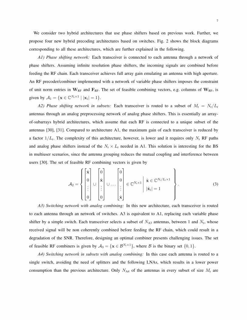
user environments where each MS can have different architectures and number of antennas.

Given the total number of measurements M = MtMr and spatial frequency resolutions Gt(≈ Nt) and

Gr(≈ Nr), one question is how to choose the number of training beamformers Mt and combiners Mr to

20

100 200 300 400 500 600 700 8000

0.1

0.2

0.3

0.4

0.5

Mutu

al C

ohere

nce

100 200 300 400 500 600 700 8000

10

20

30

40

50

Num

ber

of P

recoders

/Com

bin

ers

Number of Measurements M

Welch Bound

SC−WB

Mt

Mr

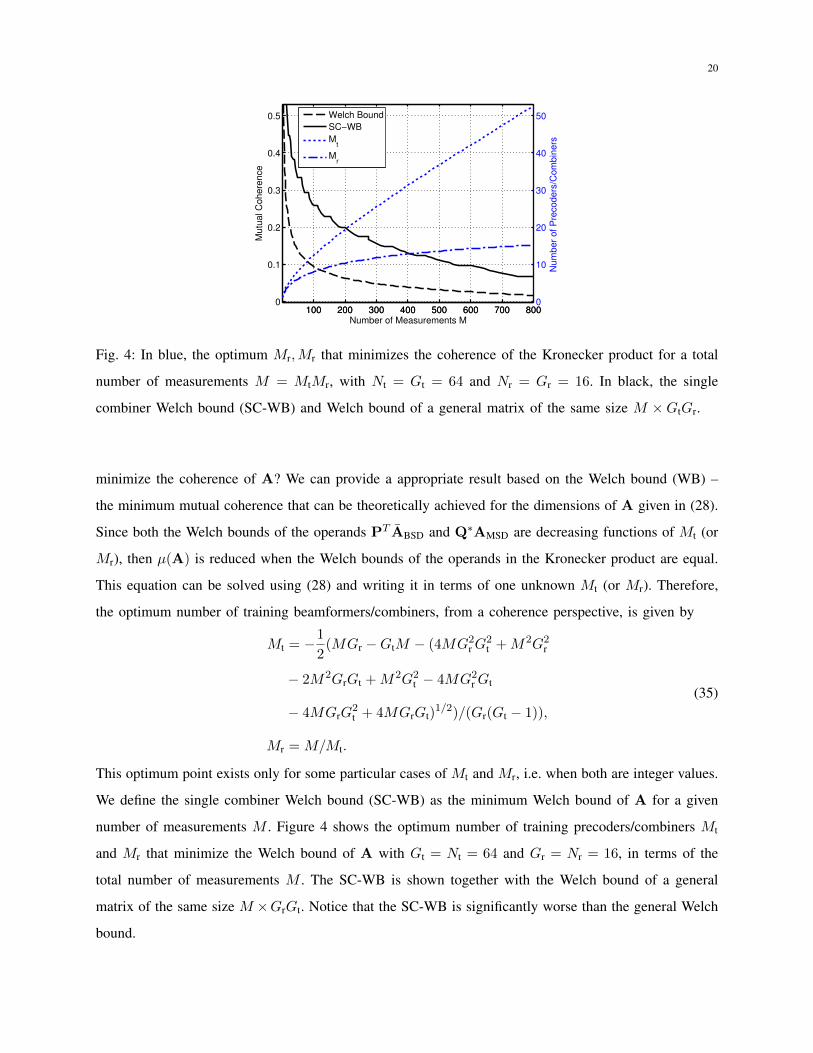
Fig. 4: In blue, the optimum Mr,Mr that minimizes the coherence of the Kronecker product for a total

number of measurements M = MtMr, with Nt = Gt = 64 and Nr = Gr = 16. In black, the single

combiner Welch bound (SC-WB) and Welch bound of a general matrix of the same size M ×GtGr.

minimize the coherence of A? We can provide a appropriate result based on the Welch bound (WB) –

the minimum mutual coherence that can be theoretically achieved for the dimensions of A given in (28).

Since both the Welch bounds of the operands PT ABSD and Q∗AMSD are decreasing functions of Mt (or

Mr), then µ(A) is reduced when the Welch bounds of the operands in the Kronecker product are equal.

This equation can be solved using (28) and writing it in terms of one unknown Mt (or Mr). Therefore,

the optimum number of training beamformers/combiners, from a coherence perspective, is given by

Mt = −1

2(MGr −GtM − (4MG2

rG2t +M2G2

r

− 2M2GrGt +M2G2t − 4MG2

rGt

− 4MGrG2t + 4MGrGt)

1/2)/(Gr(Gt − 1)),

Mr = M/Mt.

(35)

This optimum point exists only for some particular cases of Mt and Mr, i.e. when both are integer values.

We define the single combiner Welch bound (SC-WB) as the minimum Welch bound of A for a given

number of measurements M . Figure 4 shows the optimum number of training precoders/combiners Mt

and Mr that minimize the Welch bound of A with Gt = Nt = 64 and Gr = Nr = 16, in terms of the

total number of measurements M . The SC-WB is shown together with the Welch bound of a general

matrix of the same size M ×GrGt. Notice that the SC-WB is significantly worse than the general Welch

bound.

21

Given Mt and Mr, we consider the problem of designing training sequences of precoders/combiners

P and Q to minimize the coherence of A1 and A2, conforming with the hardware constraints of the

specific hybrid architecture deployed at the BS and MS. The solutions we provide in this section are

based on the virtual channel model since the extended representation using more general overcomplete

dictionaries does not lend itself to easy coherence analysis. We focus on the combining sequence design,

as the precoding problem is reciprocal.

When using switches considering the hybrid architecture A5, Q is a selection matrix with exactly

a “1” per column. The problem of selecting rows of the Fourier matrix, Q∗AMS such that the mutual

coherence of the resulting matrix is minimized is well studied. In some cases, i.e. choices of dimensions,

combinatorial sequences based on difference sets [86] are optimal and achieve the Welch bound. However,

difference sets for typical dimensions of interest in our problem rarely exist. Alternatively, combinatorial

sequences based on almost difference sets [87], can be found for a more general range of dimensions

providing near optimal coherence. In any case, numerical algorithms to create highly incoherent frames

can be applied [88] [89]. The same designs can be used for the more general hybrid architecture A4

based on switches.

When using phase shifters A1, Q is a unital matrix, i.e. a matrix with unit magnitude entries. To

the best of the authors knowledge, there are no optimal designs that achieve the Welch bound with this

special structure of the matrix. Deterministic sequences providing incoherent matrices can be built with

the same algorithm [89] since the entries in Q∗AMS are unit magnitude.

As an alternative to deterministic designs, and according to compressed sensing theory [61] [62],

random measurements from some classes of distributions (e.g. Rademacher/Bernoulli) provide incoherent

matrices satisfying the RIP with high probability. Using switches, uniform random selection of rows

from a Fourier matrix, i.e. random binary Q with exactly a “1” per column, provide equivalent matrices

satisfying the RIP [90]. Considering phase shifters A1 and A3, the results in [61] [62] suggest the use of

random sequences Q with the non zero elements chosen i.i.d. from a discrete uniform distribution taking

values {±1,±j}.

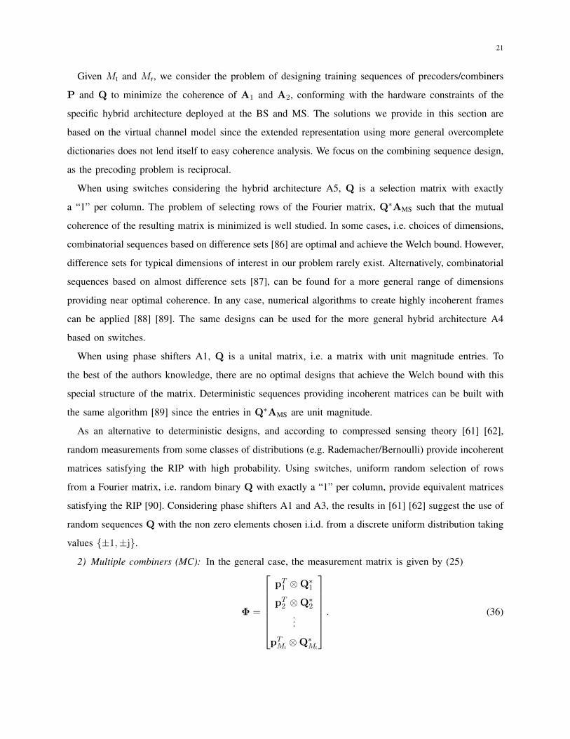
2) Multiple combiners (MC): In the general case, the measurement matrix is given by (25)

Φ =

pT1 ⊗Q∗1

pT2 ⊗Q∗2...

pTMt⊗Q∗Mt

. (36)

22

Analyzing the coherence A = ΦΨ, with Φ given by (36) is more challenging. The minimum bound on

the coherence with this model is now expected to be lower than for the single combiner case (34). This

is because we introduce in Φ extra degrees of freedom with the different Mt combiners.

Under the virtual channel model, the dictionary matrix Ψ = (ABS⊗AMS) is a Fourier matrix associated

with a 2-dimensional Fourier transform. Therefore, we suggest the use of pseudorandom sequences or

preceders/combiners with the following distributions. Using phase shifters, A1 and A3, vectors p and q

with the non zero entries i.i.d. from a uniform distribution with values {±1,±j}. Using switches, A5 and

A4, binary vectors p and q with zeros and only a “1” with its position uniformly random distributed.

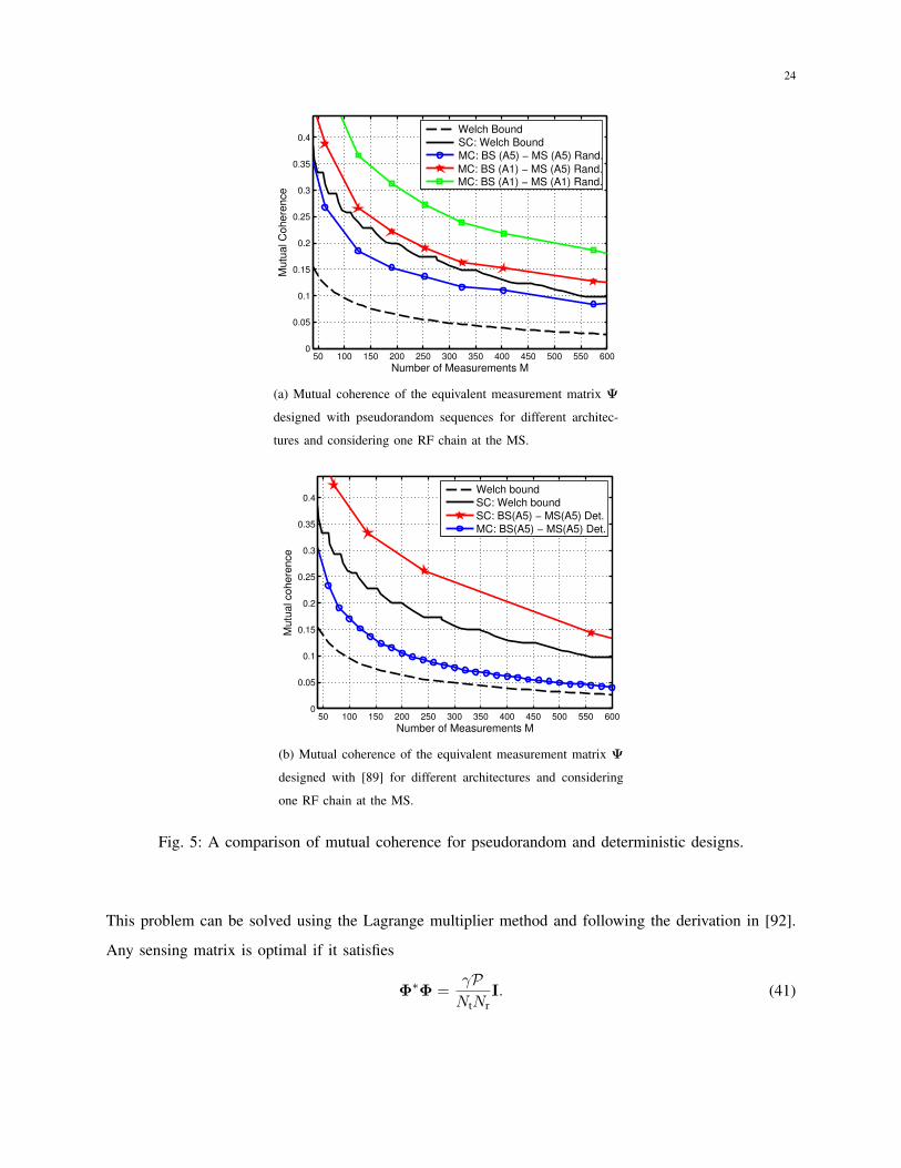
Figure 5(a) shows the mutual coherence µ(A) with Gt = Nt = 64 and Gr = Nr = 16 achieved with

the proposed pseudorandom sequences in the MC case for different combinations of hybrid architectures

at the BS and MS. Only one RF chain is considered at the MS, Lr = 1. The curves show the lowest

coherence achieved from 100 random realizations. The Welch bound and SC-WB bound are also plotted

for comparison. The achieved mutual coherence with pseudorandom sequences in the MC case with

switches at BS and MS is lower than the single combiner Welch bound, which shows the superiority

of the MC approach. Notice that switches, A5-A5, provide better coherence than phase shifters, A1-A1,

with a noticeable power consumption reduction.

As an alternative to random training sequences, it is also possible design deterministic measurement

matrices to reduce the coherence of A. In the MC case, the sequence of precoder and combiner vectors

appear coupled in the optimization problem. That means that an optimization problem needs to be solved

for each specific combination of number of antennas and RF chains deployed at the BS and MS.

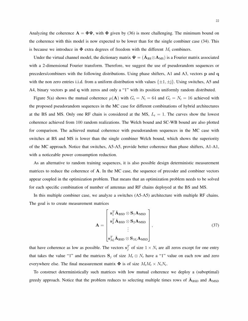
In this multiple combiner case, we analyze a switches (A5-A5) architecture with multiple RF chains.

The goal is to create measurement matrices

A =

sT1 ABSD ⊗ S1AMSD

sT2 ABSD ⊗ S2AMSD

...

sTMtABSD ⊗ SMtAMSD

, (37)

that have coherence as low as possible. The vectors sTj of size 1×Nt are all zeros except for one entry

that takes the value “1” and the matrices Sj of size Mr ⊗ Nr have a “1” value on each row and zero

everywhere else. The final measurement matrix Φ is of size MtMr ×NtNr.

To construct deterministically such matrices with low mutual coherence we deploy a (suboptimal)

greedy approach. Notice that the problem reduces to selecting multiple times rows of ABSD and AMSD

23

such that the overall coherence is minimized. For each operand at a time, in all the Kronecker products,

the algorithm selects rows iteratively such that the current coherence is maximally reduced. Convergence

is attained when a complete sweep of all sTj and Sj does not improve the coherence.

Figure 5(b) shows the mutual coherence µ(A) with Gt = Nt = 64 and Gr = 16 achieved with [89]

for different architectures and considering one RF chain at the MS. The architecture based on switches

achieves the lowest coherence. In comparison to Figure 5(b), the deterministic designs provide lower

coherence than the random sequences, below the SC-WB in most cases.

To summarize, we propose a measurement matrix structure that includes multiple combiners at the

receiver allowing therefore lower coherence than the SC case. For the single RF chain, we propose a

deterministic method to design low coherence training sequences for the architectures A1 and A5 based

on Legendre and maximum length sequences.

E. Least squares estimation

Linear least square is a conventional approach for channel estimation in MIMO systems [91] [92]. In

traditional training-based methods considering architectures with one RF chain per antenna, it is well

known that any sequence of training symbols with orthogonal rows of the same norm is optimal in the

least-squares sense [92]. In the hybrid precoding framework, the RF precoding/combining matrices must

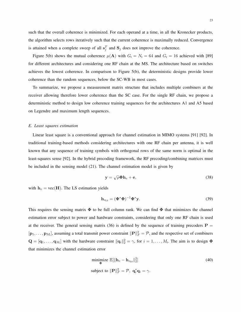
be included in the sensing model (21). The channel estimation model is given by

y =√ρΦhv + e, (38)

with hv = vec(H). The LS estimation yields

hvLS = (Φ∗Φ)−1Φ∗y. (39)

This requires the sensing matrix Φ to be full column rank. We can find Φ that minimizes the channel

estimation error subject to power and hardware constraints, considering that only one RF chain is used

at the receiver. The general sensing matrix (36) is defined by the sequence of training precoders P =

[p1, . . . ,pMt ], assuming a total transmit power constraint ‖P‖2F = P , and the respective set of combiners

Q = [q1, . . . ,qMt ] with the hardware constraint ‖qi‖22 = γ, for i = 1, . . . ,Mt. The aim is to design Φ

that minimizes the channel estimation error

minimizeΦ

E[‖hv − hvLS‖22] (40)

subject to ‖P‖2F = P, q∗iqi = γ.

24

50 100 150 200 250 300 350 400 450 500 550 6000

0.05

0.1

0.15

0.2

0.25

0.3

0.35

0.4

Number of Measurements M

Mu

tua

l C

oh

ere

nce

Welch Bound

SC: Welch Bound MC: BS (A5) − MS (A5) Rand.

MC: BS (A1) − MS (A5) Rand. MC: BS (A1) − MS (A1) Rand.

(a) Mutual coherence of the equivalent measurement matrix Ψ

designed with pseudorandom sequences for different architec-

tures and considering one RF chain at the MS.

50 100 150 200 250 300 350 400 450 500 550 6000

0.05

0.1

0.15

0.2

0.25

0.3

0.35

0.4

Number of Measurements M

Mu

tua

l co

he

ren

ce

Welch bound

SC: Welch bound

SC: BS(A5) − MS(A5) Det.

MC: BS(A5) − MS(A5) Det.

(b) Mutual coherence of the equivalent measurement matrix Ψ

designed with [89] for different architectures and considering

one RF chain at the MS.

Fig. 5: A comparison of mutual coherence for pseudorandom and deterministic designs.

This problem can be solved using the Lagrange multiplier method and following the derivation in [92].

Any sensing matrix is optimal if it satisfies

Φ∗Φ =γPNtNr

I. (41)

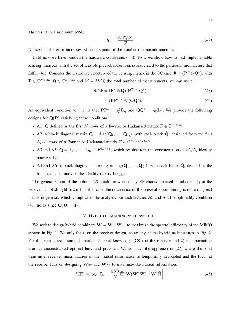
25

This result in a minimum MSE

JLS =σ2nN

2t Nr

P. (42)

Notice that the error increases with the square of the number of transmit antennas.

Until now we have omitted the hardware constraints on Φ. Now we show how to find implementable

sensing matrices with the set of feasible precoders/combiners associated to the particular architecture that

fulfill (41). Consider the restrictive structure of the sensing matrix in the SC case Φ = (PT ⊗Q∗), with

P ∈ CNt×Mt , Q ∈ CNr×Mr and M = MtMr the total number of measurements, we can write

Φ∗Φ = (P∗ ⊗Q)(PT ⊗Q∗) (43)

= (PP∗)T ⊗ (QQ∗). (44)

An equivalent condition to (41) is that PP∗ = PNr

INt and QQ∗ = γNr

INr . We provide the following

designs for Q(P) satisfying these conditions:

• A1: Q defined as the first Nr rows of a Fourier or Hadamard matrix F ∈ CMr×Mr .

• A2: a block diagonal matrix Q = diag(Q1, . . . , QLr), with each block Qi designed from the first

Nr/Lr rows of a Fourier or Hadamard matrix F ∈ CMr/Lr×Mr/Lr

• A3 and A5: Q = [INr , . . . , INr ] ∈ BNr×Mr , which results from the concatenation of Mr/Nr identity

matrices INr .

• A4 and A6: a block diagonal matrix Q = diag(Q1, . . . , QLr), with each block Qi defined as the

first Nr/Lr columns of the identity matrix IMr/Lr .

The generalization of the optimal LS condition when many RF chains are used simultaneously at the

receiver is not straightforward. In that case, the covariance of the noise after combining is not a diagonal

matrix in general, which complicates the analysis. For architectures A5 and A6, the optimality condition

(41) holds since Q∗iQi = ILr.

V. HYBRID COMBINING WITH SWITCHES

We seek to design hybrid combiners W = WRFWBB to maximize the spectral efficiency of the MIMO

system in Fig. 1. We only focus on the receiver design, using any of the hybrid architectures in Fig. 2.

For this result, we assume 1) perfect channel knowledge (CSI) at the receiver and 2) the transmitter

uses an unconstrained optimal baseband precoder. We consider the approach in [27] where the joint

transmitter-receiver maximization of the mutual information is temporarily decoupled and the focus at

the receiver falls on designing WRF and WBB to maximize the mutual information,

I(H) = log2

∣∣∣∣INt +SNRNt

H∗W(W∗W)−1W∗H

∣∣∣∣ . (45)

26

We have denoted the virtual channel H = HFopt where H is the channel matrix and Fopt is the

unconstrained optimum precoder applied at the transmitter. Given the singular value decomposition of

the channel H = UΣV∗, the optimum unconstrained combiner Wopt = UNs is given by the first Ns

singular vectors of the unitary matrix U. However, when the specific hardware constraints associated to

the mmWave architectures are considered in the design, maximizing (45) leads to a intractable constrained

optimization problem.

For the architecture A1, a low complexity hybrid precoding/combining solution was proposed in [27].

The algorithm exploits the sparse structure of the mmWave channel and formulates the design as a sparse

reconstruction problem solved with a variant of simultaneous orthogonal matching pursuit (SOMP). Other

efficient alternatives based on projections on matrices with unitary entries can be found in [25] [93].

For architectures including a subset antenna selection step, i.e. A5 or A6, the problem of designing the

optimal combiner is combinatorial. The only known exact solution is by exhaustive search, which is time

consuming. In this context, near optimal solutions can be found in [72] or [78]. The algorithm in [72]

focuses only in the design of the analog switching stage, while [78] provides a hybrid design including

the baseband combiner. The method in [72] is an incremental successive selection algorithm that at each

step activates the antenna that provides the largest increase in capacity. In the case of antenna selection

in subsets A6, the same algorithm can be applied modifying the set of feasible antennas we can select at

each iteration. That is, when one antenna form the subset i ∈ [1 . . . Lr] is activated, we have to remove

from the feasible set all the indexes associated to antennas in the subset i. The hybrid antenna selection

algorithm in [78] extends the strategy in [72] to account for the hybrid combiner design. The procedure

is summarized in Algorithm 1.

For the structures A2, A3 and A4, the joint hybrid combining design is still an open problem [30].

Further, exhaustive search is not feasible due to the extreme number of possible combinations that would

need to be checked. Alternatively, in this paper we propose two low computational complexity hybrid

combiner designs based on [27]. Assuming that W = WRFWBB can be made mathematically “close”

to the unconstrained combiner, near optimal combiners that maximize (45) can be found by minimizing

the “distance” between WRFWBB and Wopt [94]. We seek to solve the next constrained optimization

problem in terms of the Frobenius norm

minimizeWRF,WBB

‖Wopt −WRFWBB‖F

subject to WRF ∈ WRF, (46)

where WRF is the set of feasible RF combiners associated with the mmWave system architecture. Notice

27

Algorithm 1 – Hybrid Antenna SelectionInitialization: Select the first Ns rows of H according to the greedy antenna selection algorithm in

[72]. The rows are indexed in the set S and the channel matrix restricted to this support is denoted by

HS .

Iterations k = Ns + 1, . . . , Lr:

1) For each index j ∈ {1, . . . , Nr}\S:

a) Construct new channel matrix HS∪j .

b) Perform the singular value decomposition of HS∪j and set the baseband combiner WBB as the

left singular vectors.

c) Compute the mutual information (45) with HS∪j and its associated WBB. Save result in variable

C(j).

2) Choose jopt = argmaxj

C(j).

3) Update support S = S ∪ jopt.

Set the RF combiner WRF as the first Lr rows from the identity matrix IS indexed in the set S.

than solving (46) is not equivalent to maximizing the spectral efficiency. Nevertheless, the use of norm-

based designs is interesting because of its low computational complexity. Also, it has been shown in [94]

that minimizing the Frobenius norm bound results from maximizing a bound on the achievable spectral

efficiency.

To simplify the problem, we use the same strategy as [27]. Defining a dictionary of feasible combiners

D = [d1, . . . ,dNd ] of size Nr ×Nd, we solve the problem

minimizeWBB

‖Wopt −DWBB‖F

subject to ‖diag(WBBW∗BB)‖0 = Lr

‖DWBB‖2F = Ns, (47)

where ‖ · ‖0 is the `0 pseudo-norm accounting for the number of non-zero elements, WBB ∈ CNd×Ns has

only Lr non-zero rows and an energy constraint. WBB ∈ CLr×Ns is given by the Lr non-zero rows from

WBB. The solution to the problem can be obtained with the simultaneous orthogonal matching pursuit

(SOMP) in [27]. Different dictionary matrices are defined for A2, A3 and A4.

We first solve for the case of architecture A2 with each RF chain connected to a subset of antennas.

This architecture can be seen as the combination of Lr phased arrays of lower dimension, with Nr/Lr

28

antennas each. The set of feasible combiners is given by A2. From this set we create a block diagonal

dictionary matrix D = diag(D1, . . . ,DLr), with each block Di = D of size Nr/Lr × N ′d associated to

each phased array. We define D = [d(θ1), . . . , d(θN ′d)] a dictionary of steering vectors associated to each

phased array with an angular resolution N ′d. The size of the complete dictionary D is Nr × Nd with

Nd = N ′dLr.

We next propose solutions for the architectures A3 and A4. These architectures provide more flexibility

than A5 and A6 at the expenses of increasing the complexity and associated power consumption. The

ability of A3 and A4 to select and sum the contribution from a subset of antennas prior feeding the

RF chain, contributes to increase the antenna effective area and the array gain with respect to A5

and A6. Unfortunately, combining no co-phased received signals can also cause significant degradation.

Considering A3, the number of antennas in the selected subset varies from 0 to Nr, since each switch

can be activated or not. Therefore, the phase network is modulated as a binary matrix with “0” and “1”

entries. The set of feasible combiners associated with A3 is given by the set D = A3. The dimension of

the dictionary Nd grows exponentially with the number or antennas 2Nr . For a small number of antennas,

e.g., Nr = 8, the dimension Nd = 256 is reasonable. However, for higher Nr, Nd rapidly increases and

the size of the dictionary becomes intractable. Therefore, choosing a reduced dictionary of combiners is

necessary in some cases. This is an open problem that we do not consider in this paper. Similarly for

A4, the set of feasible combiners is given by A4. The architecture imposes the constraint that only one

combiner from each block in the dictionary can be selected.

VI. SIMULATIONS

In this section, we evaluate the performance of the proposed algorithms for channel estimation and

combiner optimization. First, we provide results on mean squared error of the proposed adaptive chan-

nel estimator. Second, we provide results on achievable spectral efficiency. We evaluate the trade-off

achievable spectral efficiency-power consumption with each hybrid architecture considering the power

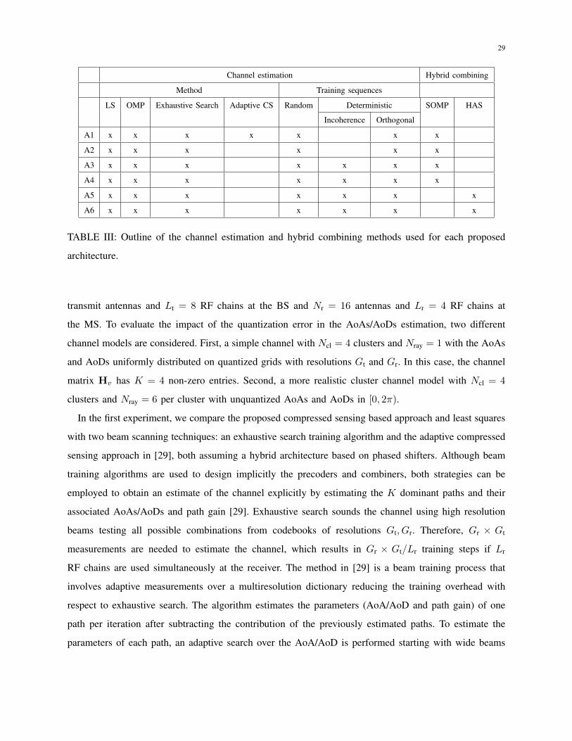
consumption model in Section III.Table III contains a summary of the channel estimation and hybrid

combining algorithms that can be used for each proposed architecture.

A. Channel estimation

First, we evaluate the channel estimation performance using the proposed compressed sensing based

channel estimation approach and the least squares solution. We use the normalized mean square error as

the performance metric NMSE = ‖H−H‖2F‖H‖2F

. We consider a single user downlink channel with Nt = 64

29

Channel estimation Hybrid combining

Method Training sequences

LS OMP Exhaustive Search Adaptive CS Random Deterministic SOMP HAS

Incoherence Orthogonal

A1 x x x x x x x

A2 x x x x x x

A3 x x x x x x x

A4 x x x x x x x

A5 x x x x x x x

A6 x x x x x x x

TABLE III: Outline of the channel estimation and hybrid combining methods used for each proposed

architecture.

transmit antennas and Lt = 8 RF chains at the BS and Nr = 16 antennas and Lr = 4 RF chains at

the MS. To evaluate the impact of the quantization error in the AoAs/AoDs estimation, two different

channel models are considered. First, a simple channel with Ncl = 4 clusters and Nray = 1 with the AoAs

and AoDs uniformly distributed on quantized grids with resolutions Gt and Gr. In this case, the channel

matrix Hv has K = 4 non-zero entries. Second, a more realistic cluster channel model with Ncl = 4

clusters and Nray = 6 per cluster with unquantized AoAs and AoDs in [0, 2π).

In the first experiment, we compare the proposed compressed sensing based approach and least squares

with two beam scanning techniques: an exhaustive search training algorithm and the adaptive compressed

sensing approach in [29], both assuming a hybrid architecture based on phased shifters. Although beam

training algorithms are used to design implicitly the precoders and combiners, both strategies can be

employed to obtain an estimate of the channel explicitly by estimating the K dominant paths and their

associated AoAs/AoDs and path gain [29]. Exhaustive search sounds the channel using high resolution

beams testing all possible combinations from codebooks of resolutions Gt, Gr. Therefore, Gr × Gt

measurements are needed to estimate the channel, which results in Gr × Gt/Lr training steps if Lr

RF chains are used simultaneously at the receiver. The method in [29] is a beam training process that

involves adaptive measurements over a multiresolution dictionary reducing the training overhead with

respect to exhaustive search. The algorithm estimates the parameters (AoA/AoD and path gain) of one

path per iteration after subtracting the contribution of the previously estimated paths. To estimate the

parameters of each path, an adaptive search over the AoA/AoD is performed starting with wide beams

30

in the early stages and narrowing the search based on the estimation outputs in the later stages to focus

only on the most promising directions. One drawback of the adaptive scheme is the need for a feedback

link between the transmitter and receiver. The required number of training steps to estimate the channel

depend on the number of dominant paths K. Considering K = 4 paths, Lr = 4 RF chains, and a

possible choice for the grid resolution Gr = Gt = 64 [29], the number of required training steps is 256(LK2[LKLr

] logL(GrK

)with L = 2

). For comparison purpose we consider the same number of training

steps and grid resolution for the proposed CS and LS schemes, which results in 256 × Lr = 1024

measurements. In this case, the training sequences for OMP are designed as pseudorandom vectors with

entries {±1,±j}. For LS, the training sequences P and Q are designed to provide orthogonality.

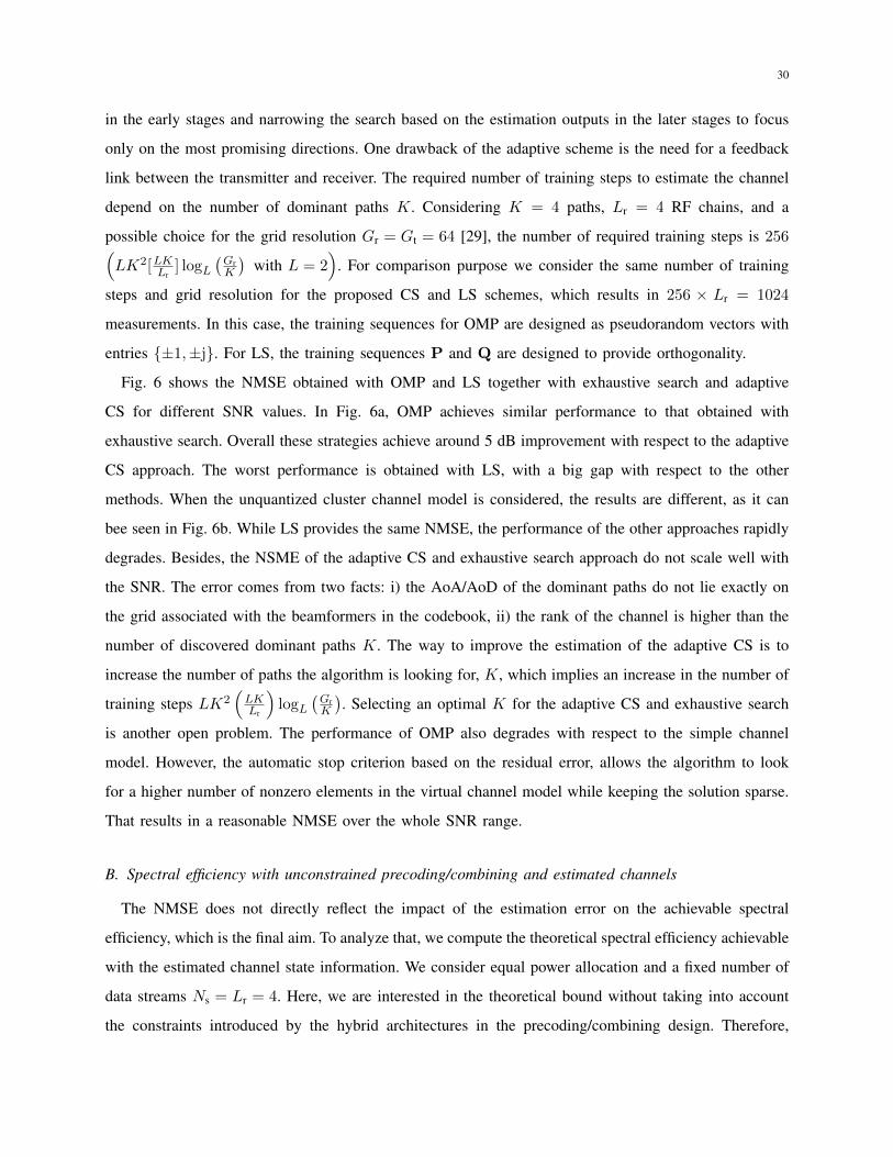
Fig. 6 shows the NMSE obtained with OMP and LS together with exhaustive search and adaptive

CS for different SNR values. In Fig. 6a, OMP achieves similar performance to that obtained with

exhaustive search. Overall these strategies achieve around 5 dB improvement with respect to the adaptive

CS approach. The worst performance is obtained with LS, with a big gap with respect to the other

methods. When the unquantized cluster channel model is considered, the results are different, as it can

bee seen in Fig. 6b. While LS provides the same NMSE, the performance of the other approaches rapidly

degrades. Besides, the NSME of the adaptive CS and exhaustive search approach do not scale well with

the SNR. The error comes from two facts: i) the AoA/AoD of the dominant paths do not lie exactly on

the grid associated with the beamformers in the codebook, ii) the rank of the channel is higher than the

number of discovered dominant paths K. The way to improve the estimation of the adaptive CS is to

increase the number of paths the algorithm is looking for, K, which implies an increase in the number of

training steps LK2(LKLr

)logL

(GrK

). Selecting an optimal K for the adaptive CS and exhaustive search

is another open problem. The performance of OMP also degrades with respect to the simple channel

model. However, the automatic stop criterion based on the residual error, allows the algorithm to look

for a higher number of nonzero elements in the virtual channel model while keeping the solution sparse.

That results in a reasonable NMSE over the whole SNR range.

B. Spectral efficiency with unconstrained precoding/combining and estimated channels

The NMSE does not directly reflect the impact of the estimation error on the achievable spectral

efficiency, which is the final aim. To analyze that, we compute the theoretical spectral efficiency achievable

with the estimated channel state information. We consider equal power allocation and a fixed number of

data streams Ns = Lr = 4. Here, we are interested in the theoretical bound without taking into account

the constraints introduced by the hybrid architectures in the precoding/combining design. Therefore,

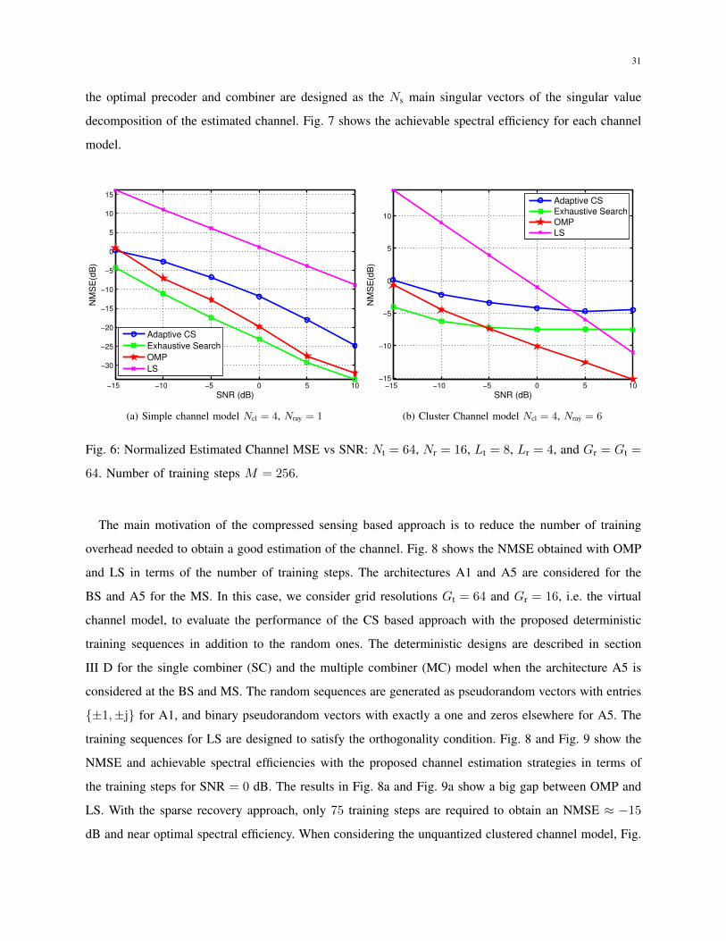
31

the optimal precoder and combiner are designed as the Ns main singular vectors of the singular value

decomposition of the estimated channel. Fig. 7 shows the achievable spectral efficiency for each channel

model.

−15 −10 −5 0 5 10

−30

−25

−20

−15

−10

−5

0

5

10

15

SNR (dB)

NM

SE

(dB

)

Adaptive CS

Exhaustive Search

OMP

LS

(a) Simple channel model Ncl = 4, Nray = 1

−15 −10 −5 0 5 10−15

−10

−5

0

5

10

SNR (dB)

NM

SE

(dB

)

Adaptive CS

Exhaustive Search

OMP

LS

(b) Cluster Channel model Ncl = 4, Nray = 6

Fig. 6: Normalized Estimated Channel MSE vs SNR: Nt = 64, Nr = 16, Lt = 8, Lr = 4, and Gr = Gt =

64. Number of training steps M = 256.

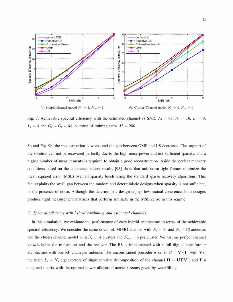
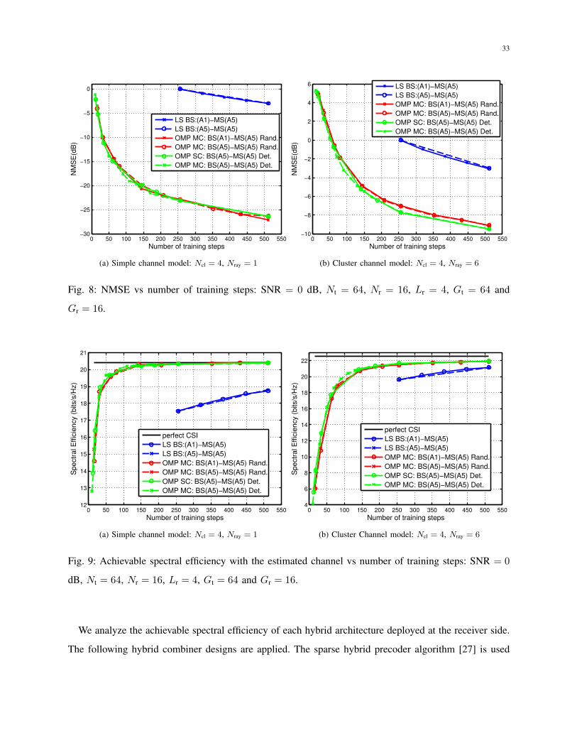
The main motivation of the compressed sensing based approach is to reduce the number of training

overhead needed to obtain a good estimation of the channel. Fig. 8 shows the NMSE obtained with OMP

and LS in terms of the number of training steps. The architectures A1 and A5 are considered for the

BS and A5 for the MS. In this case, we consider grid resolutions Gt = 64 and Gr = 16, i.e. the virtual

channel model, to evaluate the performance of the CS based approach with the proposed deterministic

training sequences in addition to the random ones. The deterministic designs are described in section

III D for the single combiner (SC) and the multiple combiner (MC) model when the architecture A5 is

considered at the BS and MS. The random sequences are generated as pseudorandom vectors with entries

{±1,±j} for A1, and binary pseudorandom vectors with exactly a one and zeros elsewhere for A5. The

training sequences for LS are designed to satisfy the orthogonality condition. Fig. 8 and Fig. 9 show the

NMSE and achievable spectral efficiencies with the proposed channel estimation strategies in terms of

the training steps for SNR = 0 dB. The results in Fig. 8a and Fig. 9a show a big gap between OMP and

LS. With the sparse recovery approach, only 75 training steps are required to obtain an NMSE ≈ −15

dB and near optimal spectral efficiency. When considering the unquantized clustered channel model, Fig.

32

−15 −10 −5 0 5 10

5

10

15

20

25

30

SNR (dB)

Spectr

al E

ffic

iency (

bits/s

/Hz)

perfect CSI

Adaptive CS

Exhaustive Search

OMP

LS

(a) Simple channel model Ncl = 4, Nray = 1

−15 −10 −5 0 5 10

5

10

15

20

25

30

35

SNR (dB)

Spectr

al E

ffic

iency (

bits/s

/Hz)

perfectCSI

Adaptive CS

Exhaustive Search

OMP

LS

(b) Cluster Channel model Ncl = 4, Nray = 6

Fig. 7: Achievable spectral efficiency with the estimated channel vs SNR: Nt = 64, Nr = 16, Lt = 8,

Lr = 4 and Gr = Gt = 64. Number of training steps M = 256.

8b and Fig. 9b, the reconstruction is worse and the gap between OMP and LS decreases. The support of

the solution can not be recovered perfectly due to the high noise power and not sufficient sparsity, and a

higher number of measurements is required to obtain a good reconstruction. Aside the perfect recovery

conditions based on the coherence, recent results [95] show that unit norm tight frames minimize the

mean squared error (MSE) over all sparsity levels using the standard sparse recovery algorithms. This

fact explains the small gap between the random and deterministic designs when sparsity is not sufficient,

in the presence of noise. Although the deterministic design enjoys low mutual coherence, both designs

produce tight measurement matrices that perform similarly in the MSE sense in this regime.

C. Spectral efficiency with hybrid combining and estimated channels

In this simulation, we evaluate the performance of each hybrid architecture in terms of the achievable

spectral efficiency. We consider the same downlink MIMO channel with Nt = 64 and Nr = 16 antennas

and the cluster channel model with Ncl = 4 clusters and Nray = 6 per cluster. We assume perfect channel

knowledge at the transmitter and the receiver. The BS is implemented with a full digital beamformer

architecture with one RF chain per antenna. The unconstrained precoder is set to F = VLrΓ, with VLr

the main Lr = Ns eigenvectors of singular value decomposition of the channel H = UΣV∗, and Γ a

diagonal matrix with the optimal power allocation across streams given by waterfilling.

33

0 50 100 150 200 250 300 350 400 450 500 550−30

−25

−20

−15

−10

−5

0

Number of training steps

NM

SE

(dB

)

LS BS:(A1)−MS(A5)

LS BS:(A5)−MS(A5)

OMP MC: BS(A1)−MS(A5) Rand.

OMP MC: BS(A5)−MS(A5) Rand.

OMP SC: BS(A5)−MS(A5) Det.

OMP MC: BS(A5)−MS(A5) Det.

(a) Simple channel model: Ncl = 4, Nray = 1

0 50 100 150 200 250 300 350 400 450 500 550−10

−8

−6

−4

−2

0

2

4

6

Number of training steps

NM

SE

(dB

)

LS BS:(A1)−MS(A5)

LS BS:(A5)−MS(A5)

OMP MC: BS(A1)−MS(A5) Rand.

OMP MC: BS(A5)−MS(A5) Rand.

OMP SC: BS(A5)−MS(A5) Det.

OMP MC: BS(A5)−MS(A5) Det.

(b) Cluster channel model: Ncl = 4, Nray = 6

Fig. 8: NMSE vs number of training steps: SNR = 0 dB, Nt = 64, Nr = 16, Lr = 4, Gt = 64 and

Gr = 16.

0 50 100 150 200 250 300 350 400 450 500 55012

13

14

15

16

17

18

19

20

21

Number of training steps

Spectr

al E

ffic

iency (

bits/s

/Hz)

perfect CSI

LS BS:(A1)−MS(A5)

LS BS:(A5)−MS(A5)

OMP MC: BS(A1)−MS(A5) Rand.

OMP MC: BS(A5)−MS(A5) Rand.

OMP SC: BS(A5)−MS(A5) Det.

OMP MC: BS(A5)−MS(A5) Det.

(a) Simple channel model: Ncl = 4, Nray = 1

0 50 100 150 200 250 300 350 400 450 500 5504

6

8

10

12

14

16

18

20

22

Number of training steps

Spectr

al E

ffic

iency (

bits/s

/Hz)

perfect CSI

LS BS:(A1)−MS(A5)

LS BS:(A5)−MS(A5)

OMP MC: BS(A1)−MS(A5) Rand.

OMP MC: BS(A5)−MS(A5) Rand.

OMP SC: BS(A5)−MS(A5) Det.

OMP MC: BS(A5)−MS(A5) Det.

(b) Cluster Channel model: Ncl = 4, Nray = 6

Fig. 9: Achievable spectral efficiency with the estimated channel vs number of training steps: SNR = 0

dB, Nt = 64, Nr = 16, Lr = 4, Gt = 64 and Gr = 16.

We analyze the achievable spectral efficiency of each hybrid architecture deployed at the receiver side.

The following hybrid combiner designs are applied. The sparse hybrid precoder algorithm [27] is used

34

to design the hybrid combiner for A1, A2, A3, and A4 as described in Section V. For the hybrid antenna

selection architectures, A5 and A6, we compute the achievable spectral efficiency of the system with the

incremental algorithm 1.

Fig. 10 shows the spectral efficiency achieved with each architecture in terms of the number of RF

chains with Ns = Lr data streams. The signal to noise ratio is fixed to SNR = 0 dB which is expected

in mmWave systems due to the large bandwidth. As expected, the hybrid architecture A1 achieves the

highest spectral efficiency with a significant gap with respect to the others. Around Lr = 6 RF chains are

sufficient to achieve the capacity of the channel. Despite A6 has lower hardware complexity than A5,

their performance almost overlaps, both achieving similar spectral efficiencies to those obtained with A2.

The architectures based on antenna selection and combining, A3 and A4, do not result in a significant

improvement with respect to simple hybrid antenna selection, A5 and A6. While A3 slightly outperforms

A2, A5 and A6 for high number of RF chains, A4 provides the worst results. The reason of this bad

performance is the specific combining algorithm used in these simulations. In fact, A4 is a more general

architecture than A6, and it should achieve at least the same spectral efficiency. Designing near optimal

precoding/combining algorithms for A2, A3 and A4 is still an open problem.

As we have seen, there is a big difference in terms of power consumption between receivers (see Fig.

3). Since power consumption is one of the main concerns in mmWave, it is interesting to analyze the

spectral efficiencies for equal power consumption. We represent in Fig. 11 the achievable bit rate in terms

of the power consumption of the RF circuit. The power consumptions are computed based on the number

of RF chains and the power model in section III. The bit rate is determined from the computed spectral

efficiencies and considering a bandwidth of BW = 500 MHz. For equal power consumption, hybrid

antenna selection architectures A5 and A6 provide the highest bit rates, with a small gap with respect to

architectures considering subsets of antennas, A2 and A4. Alternatively, the power consumption of A1

and A3 increases very rapidly with the number of RF chains, resulting in the most energy inefficient

architectures.

VII. CONCLUSIONS

In this paper we analyzed the potential of six hybrid combining architectures for mmWave commu-

nications using phase shifters or switches as main building blocks in the analog processing stage. To

complete our assessment, we developed new algorithms for channel estimation that work with all the

architectures, and specific hybrid combining algorithms for the switch architecture. We investigated the

trade-off of each architecture in terms of channel estimation performance, achievable spectral efficiencies,

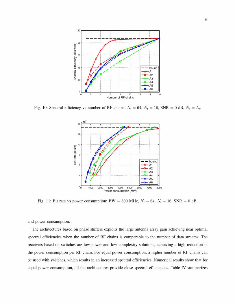
35

0 2 4 6 8 10 12 14 165

10

15

20

25

30

Number of RF chains

Spectr

al E

ffic

iency (

bits/s

/Hz)

bound

A1

A2

A3

A4

A5

A6

Fig. 10: Spectral efficiency vs number of RF chains: Nt = 64, Nr = 16, SNR = 0 dB, Ns = Lr.

0 1000 2000 3000 4000 5000 6000 7000 80002

4

6

8

10

12

14x 10

9

Power consumption [mW]

Bit R

ate

(b

its/s

)

bound

A1

A2

A3

A4

A5

A6

Fig. 11: Bit rate vs power consumption: BW = 500 MHz, Nt = 64, Nr = 16, SNR = 0 dB.

and power consumption.

The architectures based on phase shifters exploits the large antenna array gain achieving near optimal

spectral efficiencies when the number of RF chains is comparable to the number of data streams. The

receivers based on switches are low power and low complexity solutions, achieving a high reduction in

the power consumption per RF chain. For equal power consumption, a higher number of RF chains can

be used with switches, which results in an increased spectral efficiencies. Numerical results show that for

equal power consumption, all the architectures provide close spectral efficiencies. Table IV summarizes

36

the observations for the different architectures when using the same number of RF chains, emphasizing

the hardware complexity- and power consumption-spectral efficiency trade-offs. Simulations results show

that similar channel reconstruction is achieved with all the architectures and comparable to that obtained

by exhaustive search. A high number of RF chains in the mobile station reduce the number of needed

training steps at expenses of increasing the power consumption of the circuit.

Architecture Power Hardware NMSE in Spectral

consumption complexity channel estimation efficiency

A1 High High Low High

A2 Medium Medium Low Medium

A3 Medium High Low Medium

A4 Low Medium Low Medium

A5 Low Low Low Medium

A6 Low Low Low Medium

TABLE IV: Power consumption and hardware complexity versus performance of the different architec-

tures for a fixed number of RF chains.

It is of interest to extend these results using a more complete system model, including impairments of

mmWave devices like noise figure or insertion losses, which impact the actual SNR at the input of the

digital combiner. A switches-based hybrid architecture can also be considered for the transmitter, with

the resulting joint selection of the subset of antennas at transmitter and receiver.

REFERENCES

[1] Z. Pi and F. Khan, “An introduction to millimeter-wave mobile broadband systems,” IEEE Commun. Mag., vol. 49, no. 6,

pp. 101–107, 2011.

[2] T. S. Rappaport, S. Sun, R. Mayzus, H. Zhao, Y. Azar, K. Wang, G. Wong, J. Schulz, M. Samimi, and F. Gutierrez,

“Millimeter wave mobile communications for 5G cellular: It will work!” IEEE Access, vol. 1, pp. 335–349, 2013.

[3] F. Boccardi, R. W. Heath Jr., A. Lozano, T. L. Marzetta, and P. Popovski, “Five disruptive technology directions for 5G,”

IEEE Commun. Mag., vol. 52, no. 2, pp. 74–80, February 2014.

[4] S. Rangan, T. Rappaport, and E. Erkip, “Millimeter-wave cellular wireless networks: Potentials and challenges,” Proceedings

of the IEEE, vol. 102, no. 3, pp. 366–385, Mar. 2014.

[5] J. Andrews, S. Buzzi, W. Choi, S. Hanly, A. Lozano, A. Soong, and J. Zhang, “What will 5G be?” IEEE Journal on

Selected Areas in Communications, vol. 32, no. 6, pp. 1065–1082, June 2014.

[6] Federal Communications Commission, “FCC 15-138 Notice of proposed rulemaking,” October 2015.

[7] K. Venugopal, M. C. Valenti, and R. W. Heath Jr., “Interference in finite-sized highly dense millimeter wave networks,”

in Information Theory and Applications Workshop (ITA), 2015.

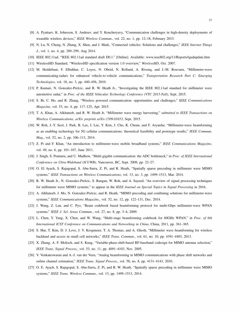
37

[8] A. Pyattaev, K. Johnsson, S. Andreev, and Y. Koucheryavy, “Communication challenges in high-density deployments of

wearable wireless devices,” IEEE Wireless Commun., vol. 22, no. 1, pp. 12–18, February 2015.

[9] N. Lu, N. Cheng, N. Zhang, X. Shen, and J. Mark, “Connected vehicles: Solutions and challenges,” IEEE Internet Things

J., vol. 1, no. 4, pp. 289–299, Aug 2014.

[10] IEEE 802.11ad, “IEEE 802.11ad standard draft D0.1.” [Online]. Available: www.ieee802.org/11/Reports/tgadupdate.htm

[11] WirelessHD Standard, “WirelessHD specification version 1.0 overview,” WirelessHD, Oct. 2007.

[12] M. Heddebaut, F. Elbahhar, C. Loyez, N. Obeid, N. Rolland, A. Rivenq, and J.-M. Rouvaen, “Millimeter-wave

communicating-radars for enhanced vehicle-to-vehicle communications,” Transportation Research Part C: Emerging

Technologies, vol. 18, no. 3, pp. 440–456, 2010.

[13] P. Kumari, N. Gonzalez-Prelcic, and R. W. Heath Jr., “Investigating the IEEE 802.11ad standard for millimeter wave

automotive radar,” in Proc. of the IEEE Vehicular Technology Conference (VTC 2015-Fall), Sept. 2015.

[14] S. Bi, C. Ho, and R. Zhang, “Wireless powered communication: opportunities and challenges,” IEEE Communications

Magazine, vol. 53, no. 4, pp. 117–125, Apr. 2015.

[15] T. A. Khan, A. Alkhateeb, and R. W. Heath Jr, “Millimeter wave energy harvesting,” submitted to IEEE Transactions on

Wireless Communications, arXiv preprint arXiv:1509.01653, Sept. 2015.

[16] W. Roh, J.-Y. Seol, J. Park, B. Lee, J. Lee, Y. Kim, J. Cho, K. Cheun, and F. Aryanfar, “Millimeter-wave beamforming

as an enabling technology for 5G cellular communications: theoretical feasibility and prototype results,” IEEE Commun.

Mag., vol. 52, no. 2, pp. 106–113, 2014.

[17] Z. Pi and F. Khan, “An introduction to millimeter-wave mobile broadband systems,” IEEE Communications Magazine,

vol. 49, no. 6, pp. 101–107, June 2011.

[18] J. Singh, S. Ponnuru, and U. Madhow, “Multi-gigabit communication: the ADC bottleneck,” in Proc. of IEEE International

Conference on Ultra-Wideband (ICUWB), Vancouver, BC, Sept. 2009, pp. 22–27.

[19] O. El Ayach, S. Rajagopal, S. Abu-Surra, Z. Pi, and R. Heath, “Spatially sparse precoding in millimeter wave MIMO

systems,” IEEE Transactions on Wireless Communications, vol. 13, no. 3, pp. 1499–1513, Mar. 2014.

[20] R. W. Heath Jr., N. Gonzalez-Prelcic, S. Rangan, W. Roh, and A. Sayeed, “An overview of signal processing techniques

for millimeter wave MIMO systems,” to appear in the IEEE Journal on Special Topics in Signal Processing in 2016.

[21] A. Alkhateeb, J. Mo, N. Gonzalez-Prelcic, and R. Heath, “MIMO precoding and combining solutions for millimeter-wave

systems,” IEEE Communications Magazine,, vol. 52, no. 12, pp. 122–131, Dec. 2014.

[22] J. Wang, Z. Lan, and C. Pyo, “Beam codebook based beamforming protocol for multi-Gbps millimeter-wave WPAN

systems,” IEEE J. Sel. Areas Commun., vol. 27, no. 8, pp. 3–4, 2009.

[23] L. Chen, Y. Yang, X. Chen, and W. Wang, “Multi-stage beamforming codebook for 60GHz WPAN,” in Proc. of 6th

International ICST Conference on Communications and Networking in China, China, 2011, pp. 361–365.

[24] S. Hur, T. Kim, D. J. Love, J. V. Krogmeier, T. A. Thomas, and A. Ghosh, “Millimeter wave beamforming for wireless

backhaul and access in small cell networks,” IEEE Trans. Commun., vol. 61, no. 10, pp. 4391–4403, 2013.

[25] X. Zhang, A. F. Molisch, and S. Kung, “Variable-phase-shift-based RF-baseband codesign for MIMO antenna selection,”

IEEE Trans. Signal Process., vol. 53, no. 11, pp. 4091–4103, Nov. 2005.

[26] V. Venkateswaran and A.-J. van der Veen, “Analog beamforming in MIMO communications with phase shift networks and

online channel estimation,” IEEE Trans. Signal Process., vol. 58, no. 8, pp. 4131–4143, 2010.

[27] O. E. Ayach, S. Rajagopal, S. Abu-Surra, Z. Pi, and R. W. Heath, “Spatially sparse precoding in millimeter wave MIMO

systems,” IEEE Trans. Wireless Commun., vol. 13, pp. 1499–1513, 2014.

38

[28] A. Alkhateeb, O. El Ayach, G. Leus, and R. Heath, “Hybrid precoding for millimeter wave cellular systems with partial

channel knowledge,” in Proc. of Information Theory and Applications Workshop (ITA), Feb 2013, pp. 1–5.

[29] A. Alkhateeb, O. E. Ayach, G. Leus, and R. W. Heath Jr., “Channel Estimation and Hybrid Precoding for Millimeter Wave

Cellular Systems,” IEEE J. Sel. Topics Signal Process., vol. 4553, pp. 831–846, 2014.

[30] S. Han, C.-L. I, Z. Xu, and C. Rowell, “Large-scale antenna systems with hybrid analog and digital beamforming for

millimeter wave 5G,” Communications Magazine, IEEE, vol. 53, no. 1, pp. 186–194, January 2015.

[31] O. El Ayach, R. Heath, S. Rajagopal, and Z. Pi, “Multimode precoding in millimeter wave mimo transmitters with multiple

antenna sub-arrays,” in Global Communications Conference (GLOBECOM), 2013 IEEE, Dec 2013, pp. 3476–3480.

[32] J. Brady, N. Behdad, and A. M. Sayeed, “Beamspace MIMO for millimeter-wave communications: System architecture,

modeling, analysis and measurements,” IEEE Trans. Antennas Propag., vol. 61, no. 7, pp. 3814–3827, July 2013.

[33] A. Poon and M. Taghivand, “Supporting and enabling circuits for antenna arrays in wireless communications,” Proc. IEEE,

vol. 100, no. 7, pp. 2207–2218, July 2012.

[34] M. Kraemer, D. Dragomirescu, and R. Plana, “A low-power high-gain LNA for the 60 GHz band in a 65 nm CMOS

technology,” in Asia-Pacific Microwave Conference, Dec 2009, pp. 1156–1159.

[35] A. Fonte, S. Saponara, G. Pinto, L. Fanucci, and B. Neri, “60-GHz single-chip integrated antenna and low noise amplifier

in 65-nm CMOS SOI technology for short-range wireless Gbits/s applications,” in International Conference on Applied

Electronics, Sept 2011, pp. 1–6.

[36] L. Liu, A. Alt, H. Benedickter, and C. Bolognesi, “Low power consumption millimeter-wave amplifiers using InP HEMT

technology,” in Microwave Workshop Series on Millimeter Wave Integration Technologies, Sept 2011, pp. 9–12.

[37] P.-Y. Chang, S.-H. Su, S. Hsu, W.-H. Cho, and J.-D. Jin, “An ultra-low-power transformer-feedback P60 GHz low-noise

amplifier in 90 nm CMOS,” IEEE Microw. Compon. Lett., vol. 22, no. 4, pp. 197–199, 2012.

[38] S. Rangan, T. Rappaport, E. Erki, Z. Latinovic, M. R. Akdeniz, and Y. Liu, “Energy efficient methods for millimeter wave

picocellular systems,” in IEEE Communication Theory Workshop, 2013.

[39] H.-K. Hong, H.-W. Kang, D.-S. Jo, D.-S. Lee, Y.-S. You, Y.-H. Lee, H.-J. Park, and S.-T. Ryu, “26.7 A 2.6b/cycle-

architecture-based 10b 1 JGS/s 15.4mW 4×-time-interleaved SAR ADC with a multistep hardware-retirement technique,”

in Solid- State Circuits Conference - (ISSCC), 2015 IEEE International, Feb 2015, pp. 1–3.

[40] B.-R.-S. Sung, D.-S. Jo, I.-H. Jang, D.-S. Lee, Y.-S. You, Y.-H. Lee, H.-J. Park, and S.-T. Ryu, “26.4 A 21fJ/conv-step 9

ENOB 1.6GS/S 2× time-interleaved FATI SAR ADC with background offset and timing-skew calibration in 45nm CMOS,”

in Solid- State Circuits Conference - (ISSCC), 2015 IEEE International, Feb 2015, pp. 1–3.

[41] N. Le Dortz, J.-P. Blanc, T. Simon, S. Verhaeren, E. Rouat, P. Urard, S. Le Tual, D. Goguet, C. Lelandais-Perrault,

and P. Benabes, “22.5 A 1.62GS/s time-interleaved SAR ADC with digital background mismatch calibration achieving

interleaving spurs below 70dBFS,” in Solid-State Circuits Conference Digest of Technical Papers (ISSCC), 2014 IEEE

International, Feb 2014, pp. 386–388.

[42] Y. Dong, R. Schreier, W. Yang, S. Korrapati, and A. Sheikholeslami, “29.2 A 235mW CT 0-3 MASH ADC achieving

-167dBFS/Hz NSD with 53MHz BW,” in Solid-State Circuits Conference Digest of Technical Papers (ISSCC), 2014 IEEE

International, Feb 2014, pp. 480–481.

[43] S. Lee, A. Chandrakasan, and H.-S. Lee, “22.4 A 1GS/s 10b 18.9mW time-interleaved SAR ADC with background timing-

skew calibration,” in Solid-State Circuits Conference Digest of Technical Papers (ISSCC), 2014 IEEE International, Feb

2014, pp. 384–385.

[44] M. Miyahara, I. Mano, M. Nakayama, K. Okada, and A. Matsuzawa, “A 2.2GS/s 7b 27.4mW time-based folding-flash ADC

39

with resistively averaged voltage-to-time amplifiers,” in IEEE International Solid-State Circuits Conference, Feb 2014, pp.

388–389.

[45] E. Janssen, K. Doris, A. Zanikopoulos, A. Murroni, G. van der Weide, Y. Lin, L. Alvado, F. Darthenay, and Y. Fregeais,

“An 11b 3.6GS/s time-interleaved SAR ADC in 65nm CMOS,” in Solid-State Circuits Conference Digest of Technical

Papers (ISSCC), 2013 IEEE International, Feb 2013, pp. 464–465.

[46] L. Kull, T. Toifl, M. Schmatz, P. Francese, C. Menolfi, M. Braendli, M. Kossel, T. Morf, T. Andersen, and Y. Leblebici,

“A 3.1mW 8b 1.2GS/s single-channel asynchronous SAR ADC with alternate comparators for enhanced speed in 32nm

digital SOI CMOS,” in Solid-State Circuits Conference Digest of Technical Papers (ISSCC), 2013 IEEE International, Feb

2013, pp. 468–469.

[47] E. Tabasy, A. Shafik, K. Lee, S. Hoyos, and S. Palermo, “A 6b 10GS/s TI-SAR ADC with embedded 2-tap FFE/1-tap

DFE in 65nm CMOS,” in VLSI Circuits (VLSIC), 2013 Symposium on, June 2013, pp. C274–C275.

[48] P. Shettigar and S. Pavan, “A 15mW 3.6GS/s CT- δσ ADC with 36MHz bandwidth and 83dB DR in 90nm CMOS,” in

Solid-State Circuits Conference Digest of Technical Papers (ISSCC), 2012 IEEE International, Feb 2012, pp. 156–158.

[49] A. L. Franc, O. H. Karabey, G. Rehder, E. Pistono, R. Jakoby, and P. Ferrari, “Compact and broadband millimeter-

wave electrically tunable phase shifter combining slow-wave effect with liquid crystal technology,” IEEE Transactions on

Microwave Theory and Techniques, vol. 61, no. 11, pp. 3905–3915, 2013.

[50] A. Natarajan, S. K. Reynolds, M.-D. Tsai, S. T. Nicolson, J.-H. C. Zhan, D. G. Kam, S. Member, D. Liu, Y.-L. O. Huang,

A. Valdes-Garcia, B. A. Floyd, and S. Member, “A Fully-Integrated 16-Element Phased-Array Communications,” vol. 46,

no. 5, pp. 1059–1075, 2011.

[51] W. T. Li, Y. C. Chiang, J. H. Tsai, H. Y. Yang, J. H. Cheng, and T. W. Huang, “60-GHz 5-bit phase shifter with integrated

VGA phase-error compensation,” IEEE Transactions on Microwave Theory and Techniques, vol. 61, no. 3, pp. 1224–1235,

2013.

[52] M. Uzunkol and G. Rebeiz, “A 65 GHz LNA/Phase Shifter with 4.3 dB NF using 45 nm CMOS SOI,” IEEE Microw.

Compon. Lett., vol. 22, no. 10, pp. 530–532, Oct 2012.

[53] J.-L. K. et al., “60-GHz four-element phased-array transmit/receive system-in-package using phase compensation techniques

in 65-nm Flip-Chip CMOS process,” IEEE Trans. Microw. Theory and Techn., vol. 60, no. 3, pp. 743–756, March 2012.

[54] S. Y. Kim, D. W. Kang, K. J. Koh, and G. M. Rebeiz, “An improved wideband all-pass I/Q network for millimeter-wave

phase shifters,” IEEE Transactions on Microwave Theory and Techniques, vol. 60, no. 11, pp. 3431–3439, 2012.

[55] Y. Yu, P. G. M. Baltus, A. De Graauw, E. Van Der Heijden, C. S. Vaucher, and A. H. M. Van Roermund, “A 60 GHz phase

shifter integrated with LNA and PA in 65 nm CMOS for phased array systems,” IEEE Journal of Solid-State Circuits,

vol. 45, no. 9, pp. 1697–1709, 2010.

[56] K. J. Kim, K. H. Ahn, T. H. Lim, H. C. Park, and J. W. Yu, “A 60 GHz wideband phased-array LNA with short-stub

passive vector generator,” IEEE Microwave and Wireless Components Letters, vol. 20, no. 11, pp. 628–630, 2010.

[57] D. Liu, U. Pfeiffer, J. Grzyb, and B. Gaucher, Advanced Millimeter-wave Technologies: Antennas, Packaging and Circuits.

Wiley, 2009.

[58] L. A. Belov, S. M. Smolskiy, and V. N. Kochemasov, Handbook of RF, Microwave, and Millimeter-Wave Components.

Artech House, 2012.

[59] R. Schmid, P. Song, C. Coen, A. Ulusoy, and J. Cressler, “On the analysis and design of low-loss single-pole double-throw

W-band switches utilizing saturated SiGe HBTs,” IEEE Trans. Microw. Theory and Techn., vol. 62, no. 11, pp. 2755–2767,

Nov 2014.

40

[60] V. Ziegler, R. Deufel, C. Wolk, C. Gassler, J. Dickmann, and H. Schumacher, “Metamorphic pin diodes for high isolation

and low power consumption millimetre-wave switching MMICs,” Electronics Letters, vol. 36, no. 18, pp. 1556–1557, Aug

2000.

[61] W. U. Bajwa and J. Haupt, “Compressed channel sensing: A new approach to estimating sparse multipath channels,” Proc.

IEEE, vol. 98, no. 6, pp. 1058–1076, Jun. 2010.

[62] D. Ramasamy, S. Venkateswaran, and U. Madhow, “Compressive adaptation of large steerable arrays,” 2012 Information

Theory and Applications Workshop, pp. 234–239, Feb. 2012.

[63] J. Lee, G. Gye-Tae, and Y. H. Lee, “Exploiting spatial sparsity for estimating channels of hybrid MIMO systems in

millimeter wave communications,” in IEEE Globecom, 2014.

[64] D. E. Berraki, S. M. D. Armour, and A. R. Nix, “Application of compressive sensing in sparse spatial channel recovery

for beamforming in mmWave outdoor systems,” in Proc. IEEE Wireless Communications and Networking Conference

(WCNC), Apr. 2014, pp. 887–892.

[65] A. Alkhateeb, G. Leus, and R. W. Heath Jr., “Compressed-sensing based multi-user millimeter wave systems: How many

measurements are needed?” in Proc. of the IEEE International Conf. on Acoustics, Speech and Signal Processing (ICASSP),

April 2015.

[66] M. Malloy and R. Nowak, “Near-optimal adaptive compressed sensing,” Information Theory, IEEE Transactions on, vol. 60,

no. 7, pp. 4001–4012, July 2014.

[67] L. Welch, “Lower bounds on the maximum cross correlation of signals (Corresp.),” IEEE Trans. Inf. Theory, vol. 20, 1974.

[68] F. Sohrabi and W. Yu, “Hybrid digital and analog beamforming design for large-scale MIMO systems,” in Proc. of the

IEEE International Conf. on Acoustics, Speech and Signal Processing, April 2015.

[69] C. Rusu, R. Mendez-Rial, N. Gonzalez-Prelcic, and R. W. Heath Jr, “Low complexity hybrid sparse precoding and

combining in millimeter wave MIMO systems,” in Proc. IEEE Int. Conf. on Commun. (ICC). IEEE, Jun. 2015.

[70] S. Sanayei and A. Nosratinia, “Antenna selection in mimo systems,” Communications Magazine, IEEE, vol. 42, no. 10,

pp. 68–73, Oct 2004.

[71] A. Molisch and M. Win, “Mimo systems with antenna selection,” Microwave Magazine, IEEE, vol. 5, no. 1, pp. 46–56,

Mar 2004.

[72] M. Gharavi-Alkhansari and A. B. Gershman, “Fast antenna subset selection in MIMO systems,” IEEE Trans. Signal

Process., vol. 52, no. 2, pp. 339–347, 2004.

[73] S. Sanayei and A. Nosratinia, “Antenna selection in MIMO systems,” IEEE. Commun. Mag., no. October, pp. 68–73, 2004.

[74] Y.-Y. Lee, C.-H. Wang, and Y.-H. Huang, “A hybrid RF/baseband precoding processor based on parallel-index-selection

matrix-inversion-bypass simultaneous orthogonal matching pursuit for millimeter wave MIMO systems,” IEEE Trans. Signal

Process., vol. 63, no. 2, pp. 305–317, Jan 2015.

[75] T. S. Rappaport, F. Gutierrez, E. Ben-Dor, J. N. Murdock, Y. Qiao, and J. I. Tamir, “Broadband millimeter-wave

propagation measurements and models using adaptive-beam antennas for outdoor Urban cellular communications,” IEEE

Trans. Antennas Propag., vol. 61, pp. 1850–1859, 2013.

[76] A. M. Sayeed, “Deconstructing multiantenna fading channels,” IEEE Trans. Signal Process., vol. 50, no. 10, pp. 2563–2579,

2002.

[77] A. Alkhateeb, R. W. Heath Jr., and G. Leus, “Compressed-sensing based multi-user millimeter wave systems: How many

measurements are needed?” April 2015.

41

[78] R. Mendez-Rial, C. Rusu, A. Alkhateeb, N. Gonzalez-Prelcic, and R. W. Heath Jr., “Channel estimation and hybrid

combining for mmwave: Phase shifters or switches?” in Information Theory and Applications Workshop (ITA), 2015.

[79] G. Taubock, F. Hlawatsch, D. Eiwen, and H. Rauhut, “Compressive estimation of doubly selective channels in multicarrier

systems: Leakage effects and sparsity-enhancing processing,” IEEE J. Sel. Topics Signal Process., vol. 4, pp. 255–271,

2010.

[80] J. Tropp, “Greed is good: Algorithmic results for sparse approximation,” IEEE Trans. Inf. Theory, vol. 50, no. 10, pp.

2231–2242, 2004.

[81] T. T. Cai, L. Wang, and G. Xu, “Stable recovery of sparse signals and an oracle inequality,” IEEE Trans. Inf. Theory,

vol. 56, pp. 3516–3522, 2010.

[82] T. T. Cai and L. Wang, “Orthogonal matching pursuit for sparse signal recovery with noise,” IEEE Trans. Inf. Theory,

vol. 57, no. 7, pp. 4680–4688, 2011.

[83] E. Candes, J. Romberg, and T. Tao, “Robust uncertainty principles: Exact signal reconstruction from highly incomplete

frequency information,” IEEE Trans. Inf. Theory, vol. 52, pp. 489–509, 2006.

[84] ——, “Stable signal recovery from incomplete and inaccurate measurements,” Communications on Pure and Applied

Mathematics, vol. 59, pp. 1207–1223, 2006.

[85] S. Jokar and V. Mehrmann, “Sparse solutions to underdetermined Kronecker product systems,” Linear Algebra and Its

Applications, vol. 431, no. 12, pp. 2437–2447, 2009.

[86] P. Xia, Z. Shengli, and G. B. Giannakis, “Achieving the welch bound with difference sets,” IEEE Trans. Inf. Theory,

vol. 52, no. 5, pp. 1900–1907, 2005.

[87] K. Nowak, “A survey on almost difference sets,” arXiv:1409.0114, 2014.

[88] G. Xu and Z. Xu, “Compressed Sensing Matrices from Fourier Matrices,” IEEE Transactions on Information Theory,

vol. 61, no. 1, pp. 469–478, 2015.

[89] C. Rusu, N. Gonzalez-Prelcic, and R. W. Heath Jr., “Algorithmic construction of incoherent frames under various design

constraint,” 2015.

[90] S. Foucart and H. Rauhut, A Mathematical Introduction to Compressive Sensing. Birkhuser Basel, 2013.

[91] E. Karami, “Tracking Performance of Least Squares MIMO Channel Estimation Algorithm,” IEEE Transactions on

Communications, vol. 55, no. 11, pp. 2201–2209, 2007.

[92] M. Biguesh and A. B. Gershman, “Training-based MIMO channel estimation: A study of estimator tradeoffs and optimal

training signals,” IEEE Trans. Signal Process., vol. 54, pp. 884–893, 2006.

[93] R. Mendez-Rial, C. Rusu, N. Gonzalez-Prelcic, and R. W. Heath Jr, “Dictionary-free hybrid precoders and combiners for

mmwave MIMO systems,” SPAWC, 2015.

[94] O. E. Ayach, R. W. Heath, S. Abu-Surra, S. Rajagopal, and Z. Pi, “Low complexity precoding for large millimeter wave

MIMO systems,” IEEE International Conference on Communications, pp. 3724–3729, Jun. 2012.

[95] C. Wei, M. R. D. Rodrigues, and I. J. Wassell, “On the use of unit-norm tight frames to improve the average mse

performance in compressive sensing applications,” IEEE Signal Processing Letters, vol. 19, pp. 8–11, 2012.