Embed Size (px)
Citation preview
Hydraulic hazard exposure of humans swept away in a whitewater river 1
2
Michael A Strom1*, Gregory B Pasternack1, Scott G Burman1, Helen E Dahlke1, Samuel 3
Sandoval-Solis1 4
5
*Corresponding author 6
E-mail address: [email protected] 7
8
1Department of Land, Air and Water Resources, University of California, Davis, One 9
Shields Avenue, Davis, CA, USA 95616 10
11
12
Cite as: Strom, M. A., Pasternack, G. B., Burman, S. G., Dahlke, H. E., Sandoval-Solis, 13
S. 2017. Hydraulic hazard exposure of humans swept away in a whitewater river. 14
Natural Hazards. doi:10.1007/s11069-017-2875-6 15
16
The final publication is available at Springer via http://dx.doi.org/10.1007/s11069-017-17
2875-6 18
19

Abstract 20
Despite many deaths annually worldwide due to floods, no strategy exists to 21
mechanistically map hydraulic hazards people face when entrained in a river. Previous 22
work determined water depth–velocity product thresholds for human instability from 23
standing or walking positions. Because whitewater rivers attract diverse recreation that 24
risks entraining people into hazardous flow, this study takes the next step by predicting 25
the hazard pattern facing people swept away. The study site was the 12.2-km bedrock–26
alluvial upper South Yuba River in the Sierra Nevada Mountains. A novel algorithm was 27
developed and applied to two-dimensional hydrodynamic model outputs to delineate 28
three hydraulic hazard categories associated with conditions for which people may 29
be unable to save themselves: emergent unsavable and steep emergent surfaces, 30
submerged unsavable surfaces, and hydraulic jumps. Model results were used to 31
quantify exposure of both an upright and supine entrained person to collision and body 32
entrapment hazards. Hazard exposure was expressed with two metrics: passage 33
proximity (how closely a body approached a hazard) and reaction time (time available to 34
respond to and avoid a hazard). Hazard exposure maps were produced for multiple 35
discharges, and the areal distributions of exposure were synthesized for the river 36
segment. Analyses revealed that the maximum hazard exposure occurred at an 37
intermediate discharge. Additionally, longitudinal profiles of the results indicated both 38
discharge-dependent and discharge-independent hazards. Relative to the upright body, 39
the supine body was overall exposed to less dangerous channel regions in passage 40
down the river, but experienced more abrupt encounters with the danger that did occur. 41
Keywords: Hydraulic hazards; River rapids; Floods; Hydraulic jumps; Whitewater 42
1. Introduction 43
Worldwide, more than 175,000 people were killed by freshwater floods from 1975 44
to 2001 (Jonkman 2005), and a review of river flood events found that the majority of 45
fatalities stemmed from drowning or physical trauma (Jonkman and Kelman 2005). 46
Current strategies for flow-related, or hydraulic, hazard assessments involve identifying 47
depth–velocity product thresholds above which humans lose stability from either a 48
standing or walking position. Theoretical studies have characterized friction (sliding) and 49
moment (toppling) instability mechanisms (Keller and Mitsch 1993; Lind et al. 2004; 50
Jonkman and Penning-Rowsell 2008; Xia et al. 2014), and experimental studies have 51
been used to evaluate the predicted thresholds for the occurrence of these mechanisms 52
(Foster and Cox 1973; Abt et al. 1989; Takahashi et al. 1992; Karvonen et al. 2000; 53
Jonkman and Penning-Rowsell 2008; Cox et al. 2010; Russo et al. 2013; Xia et al. 54
2014). Factors influencing the onset of human instability in a flow include body weight, 55
height, clothing, ground surface composition, slope, entrained debris, flow turbulence, 56
fluid density, psychology, experience, and other variables (Karvonen et al. 2000; 57
Chanson et al. 2014; Milanesi et al. 2015). 58
Relative to investigating the conditions for instability, simulating the fate of people 59
following the loss of stability has received little attention. McCarroll et al. (2015) 60
modeled the transport of bathers in a rip current as a series of particles in a flow field 61
and simulated multiple escape strategies to evaluate their success. The present study 62
also sought to predict the fate of people carried away in a flow, but in a whitewater river 63
that hosts multiple forms of recreation. The hydraulic hazard exposure of people swept 64
down a river was described, defined herein as the potential for entrained bodies to 65
encounter hazards and incur harm in the form of drowning or physical trauma. To be 66
conservative, it was assumed that any hazard exposure could produce harm and 67
therefore needed to be documented. 68
1.1. Whitewater river hydraulic hazards 69
Whitewater rivers contain a variety of elements that create channel complexity 70
and rapids that can be hazardous to people. Boulders transported into a channel by 71
tributaries and landsliding from cliff faces have been found to produce rapids (Dolan et 72
al. 1978; Graf 1979; Webb et al. 1988). Debris flow fan deposits at the mouths of 73
tributaries can be reworked by main channel flows to create downstream rock gardens 74
and additional rapids (Kieffer 1985; Webb et al. 1989). These rock features impose 75
lateral and vertical flow constrictions that generate several wave types, including abrupt 76
transitions from supercritical to subcritical flow in the form of hydraulic jumps (Leopold 77
1969; Kieffer 1985). The diverse morphologies and arrangements of rock elements and 78
their control on flow served as the basis for the classification of different channel units in 79
bedrock rivers (Grant et al. 1990). The flow features associated with whitewater rivers 80
also spurred the development of the International Scale of River Difficulty in the 1950s 81
by the association American Whitewater in an effort to classify and convey the 82
challenges of traversing rapids. The rating system was revised in 1998 to focus less on 83
describing individual hazards and more on expressing the intangible measure of overall 84
rapid difficulty (Belknap 1998). Consequently, by its design, the system offers no more 85
than qualitative characterizations of each of the six difficulty ratings at the scale of 86
individual rapids. 87
As an example of a hazardous whitewater river setting, the Mather Gorge and its 88
Great Falls on the Potomac River upstream of Washington, D.C. are notorious for 89
deaths due to deceptive waters and close proximity to a large urban center from which 90
people with varying hazard awareness travel for recreation. The Washington Post 91
published a visually interactive overview of hydraulic hazards present in this canyon 92
where 27 people died 2001–2013 (The perils at Great Falls, The Washington Post, 93
2013) and 51% of river accidents here are fatal, with 72% of these incidents originating 94
from shoreline-based activities that are not related to boating (Potomac River Gorge 95
Safety Press Conference, National Park Service, 2013). After getting swept from shore 96
or falling out of a craft, collisions and/or entrapment with emergent or submerged rocks 97
can cause physical trauma and/or drowning, and entrapment inside hydraulic jumps 98
exhibiting strong multiphase flow recirculation can hold a body underwater until death. 99
Although this study focuses on whitewater rivers, similar hydraulic hazards occur 100
during urban flooding, including during storm surges and tsunamis. Instead of 101
hazardous interactions with boulders and bedrock, collisions with and entrapment by 102
features of the urban landscape can cause physical trauma and drowning (Jonkman 103
2005). Both whitewater rivers and urban floods can also contain floating debris that 104
present an additional hazard, and Penning-Rowsell et al. (2005) introduced a flood 105
hazard equation that uses a debris factor to account for this. Thus, the new methods 106
presented in this study have broader significance to understanding natural flood 107
hazards. 108
1.2. Meter-scale river maps and models 109
Characterizing the exposure of humans to hydraulic hazards required a digital 110
terrain model of the topo-bathymetric surface and a hydrodynamic model with a 111
resolution commensurate with the human scale. To determine the local occurrence of 112
hydraulic hazards and then aggregate the results to coarser scales, data collection and 113
mechanistic modeling methods that resolve meter-scale variations were required. 114
Meter-scale data are increasingly available for free (e.g., 115
http://www.opentopography.org) or can be collected at a rapidly decreasing cost with 116
increasing detail. Key technologies include airborne LiDAR mapping of the terrestrial 117
river corridor (Lane and Chandler 2003; Hilldale and Raff 2008), airborne bathymetric 118
LiDAR mapping of shallow, clear water (McKean et al. 2008), and boat-based 119
echosounding of the subaqueous riverbed (Vilming 1998; Muste et al. 2012). To 120
characterize spatially distributed, meter-scale river hydraulics over tens of kilometers at 121
many discharges, two-dimensional (2D) depth-averaged hydrodynamic modeling was 122
used. 123
1.3. Study objectives 124
For a segment of the upper South Yuba River (SYR) in Northern California, the 125
objectives of this study were to (1) conceptualize different hydraulic hazards and 126
delineate their locations for multiple discharges, (2) design hydraulics-based metrics to 127
quantify and map the exposure of an entrained human body in the upright and supine 128
positions to these hazards, and (3) determine trends in the hazards as a function of 129
discharge and longitudinal position in the river. This study introduces a systematic, 130

objective, and detailed approach to quantifying and mapping hydraulic hazard exposure 131
within the process-based research paradigm. 132
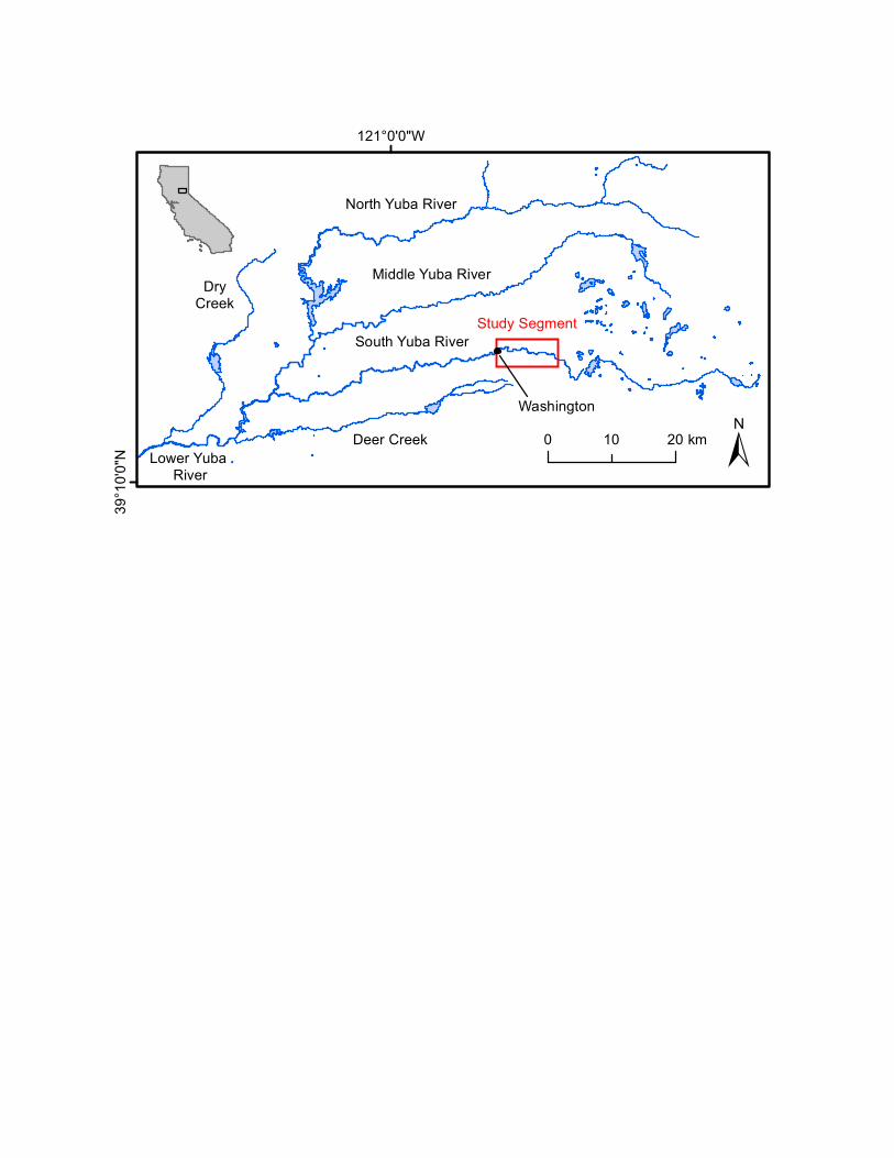
2. Study area 133
The 12.2-km SYR study segment was located on the west side of the Sierra 134
Nevada Mountains beginning at the coordinates {39°20′48.34″N, 120°41′ 37.55″W} and 135
terminating at the town of Washington, California, at the coordinates {39°21′28.55″N, 136
120°48′11.54″W} (Fig. 1). A thorough description of the study segment is available in 137
Pasternack and Senter (2011), so only the essential details are provided here for 138
brevity. This region is characterized by a Mediterranean climate with an average annual 139
precipitation of 173.9 cm (Western Regional Climate Center) for 1914–2003 at Lake 140
Spaulding, 8 km upstream of the upper extent of the study segment. The drainage area 141
above Washington, CA, is 512.8 km2 with 310.8 km2 captured by Spaulding Dam. 142
Regulated releases and unregulated spills occur at the dam. The average daily flow for 143
1965–2014 measured just downstream at Langs Crossing (USGS gage 11414250) was 144
3.03 m /s, while the average daily flow at Washington (USGS gage 11417000) for 145
1942–1972 was 8.44 m3/s. Inadequate historical flow records prior to flow regulation, 146
periodic, complex changes to flow regulation, interdecadal trends in the hydrologic 147
regime due to forest cover changes, and cumulative, unabated geomorphic impacts 148
from multiple, severe anthropogenic activities, such as hydraulic mining of hillsides, 149
preclude reasonable determination of bankfull discharge. Four tributaries drain into the 150
study segment and two more do so above the study segment but below the dam. The 151
maximum elevation in the watershed is 2552 m above mean sea level, and the channel 152
bed elevation within the study segment ranges from ~780 to 1015 m. Bed material 153
±
South Yuba River
Middle Yuba River
North Yuba River
0 2010 km
Study Segment
121°0'0"W39
°10'0
"N Lower Yuba River
Deer Creek
DryCreek
Washington
spans sand to large boulders, and extensive bedrock outcrops are associated with 154
canyons and pools. Hydraulic mining was performed at multiple sites within the study 155
segment and has contributed sediment to the channel (Pasternack and Senter 2011). 156
3. Methods 157
This article presents an approach to evaluate hydraulic hazards (Sects. 3.2 – 3.4) 158
and then applies it to a case study to find new insights about whitewater rivers. A high-159
resolution DEM and 2D hydrodynamic model were used in this study, but those 160
elements and data underpinning them are not the focus herein. Increasingly, the 161
frontiers of river science are being built upon such models (e.g., Hauer et al. 2009; 162
Wyrick and Pasternack 2014; Gonzalez and Pasternack 2015; Strom et al. 2016), with 163
the aim of journal articles to present the novel developments. The underpinnings and 164
validation of the data and model are important background and thus explained in Online 165
Resource 1 to keep the article’s focus on new science. 166
3.1. Meter-scale data and hydrodynamic model 167
Field data were used to characterize geomorphic, hydrologic, and hydraulic 168
attributes of the remote and hazardous SYR at ~1-5 m resolution, including 2D 169
hydrodynamic modeling. An airborne LiDAR survey mapped 34,113 large, emergent 170
boulders within the wetted area at the heavily regulated low base flow−an important and 171
unique aspect of this study in order to address hydraulic hazards (Pasternack and 172
Senter 2011). 173
A previously peer-reviewed, meter-scale 2D hydrodynamic model of the SYR 174
was used in this study. Three-dimensional (3D) hydrodynamic models are available, but 175

have high computational demands for the >10 km range and 1-m resolution needed. 176
The new science and methods in this study do not depend on whether the model is 2D 177
or 3D, just that the outputs are meter-scale to resolve hydraulic hazards. Scientific 178
exploration with 3D models is ongoing and can be expected to eventually surpass the 179
current use of 2D models. The use of a morphodynamic model was also not considered, 180
because this study only investigated a range of flows for which large boulders would not 181
be in transport (Pasternack and Senter 2011). This decision was made because most 182
recreational risk and mortality occur at flows when coarse sediment is not in motion. 183
Non-recreational mortality often does occur during extreme floods that are channel-184
changing events, and this study does not address such geomorphic dynamism. The 185
Sedimentation and River Hydraulics Two-dimensional Model (Lai 2008) solved the 186
depth-averaged St. Venant equations using the finite-volume method to simulate both 187
subcritical and supercritical flows, which was key to predicting the occurrence of 188
hydraulic jump hazards. Model validation is detailed in Online Resource 1. Validation 189
results were within accepted standards (e.g., Gard 2003; Pasternack et al. 2006b; 190
Reinfelds et al. 2010). 191
The assumption of 2D flow is strictly violated through waterfalls and inside 192
hydraulic jumps, but these are a small fraction of the model domain. Additionally, our 193
field experience with evaluating model performance for point velocity in waterfalls of the 194
SYR revealed that the problem primarily affects the positioning of the peak velocity in a 195
vertical drop and not the presence and position of the hydraulic jump, which were more 196
critical for this study. Support for this viewpoint and application exists in the literature 197
where 2D models have been used to investigate settings with complex 3D flows, such 198
as dam-break-induced floods (Peng 2012), spillway flow (Ying and Wang 2012), and 199
other boulder-bed streams (Harrison and Keller 2007). Therefore, 2D modeling was 200
appropriate to use for this purpose of mapping hydraulic jumps. 201
Model results used in this study were for snowmelt-driven flows of 15, 31, 85, 202
and 196 m3/s, which correspond to the 70th, 82nd, 89th, and 92nd percentile values, 203
respectively, for the daily mean discharge series at the Langs Crossing gage. These 204
discharges are also higher than the daily mean flow reported for the Washington gage 205
at the downstream end of the segment, and they span the approximate discharge range 206
across which kayakers and rafters have been reported to run the river (Jolly Boys and 207
Golden Quartz runs of the South Yuba River, A Wet State, 208
http://www.awetstate.com/1Alph.html#CA). 209
3.2. Human body abstraction 210
A human body can assume multiple positions in a flow, which changes the 211
exposure to surrounding hazards. Floating with feet pointed downstream in the supine 212
position is a commonly reported strategy for safe passage known as defensive 213
swimming (Whitewater skill: How to swim, Rapid Media, 214
https://www.rapidmedia.com/rapid/categories/skills/1288-whitewater-skill-how-to-215
swim.html), while floating with legs extended downward into the water column may be 216
used by someone who does not have this training or is otherwise unable to maintain the 217
supine position. While there are positions that are intermediate between these two, the 218
supine and upright positions correspond to the end members of exposure to hazards 219
beneath the water surface assuming that the head remains unsubmerged. The supine 220
position maximizes the distance between the body and a submerged hazard while the 221
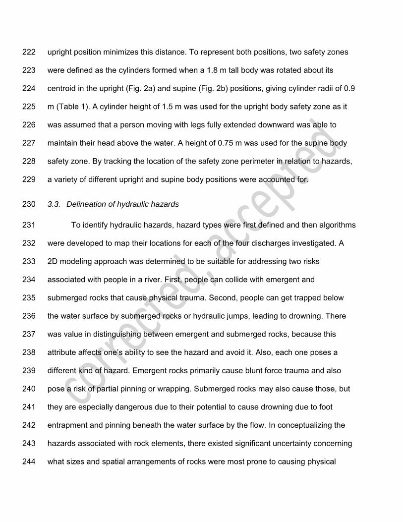
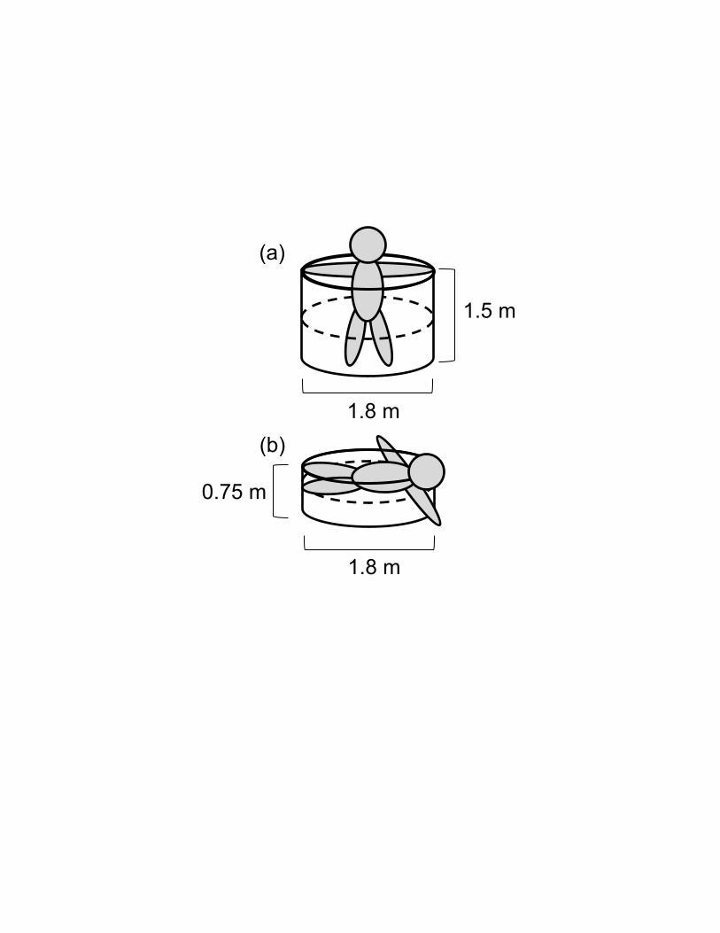
upright position minimizes this distance. To represent both positions, two safety zones 222
were defined as the cylinders formed when a 1.8 m tall body was rotated about its 223
centroid in the upright (Fig. 2a) and supine (Fig. 2b) positions, giving cylinder radii of 0.9 224
m (Table 1). A cylinder height of 1.5 m was used for the upright body safety zone as it 225
was assumed that a person moving with legs fully extended downward was able to 226
maintain their head above the water. A height of 0.75 m was used for the supine body 227
safety zone. By tracking the location of the safety zone perimeter in relation to hazards, 228
a variety of different upright and supine body positions were accounted for. 229
3.3. Delineation of hydraulic hazards 230
To identify hydraulic hazards, hazard types were first defined and then algorithms 231
were developed to map their locations for each of the four discharges investigated. A 232
2D modeling approach was determined to be suitable for addressing two risks 233
associated with people in a river. First, people can collide with emergent and 234
submerged rocks that cause physical trauma. Second, people can get trapped below 235
the water surface by submerged rocks or hydraulic jumps, leading to drowning. There 236
was value in distinguishing between emergent and submerged rocks, because this 237
attribute affects one’s ability to see the hazard and avoid it. Also, each one poses a 238
different kind of hazard. Emergent rocks primarily cause blunt force trauma and also 239
pose a risk of partial pinning or wrapping. Submerged rocks may also cause those, but 240
they are especially dangerous due to their potential to cause drowning due to foot 241
entrapment and pinning beneath the water surface by the flow. In conceptualizing the 242
hazards associated with rock elements, there existed significant uncertainty concerning 243
what sizes and spatial arrangements of rocks were most prone to causing physical 244
1.5 m
(a)
1.8 m
0.75 m
(b)
1.8 m
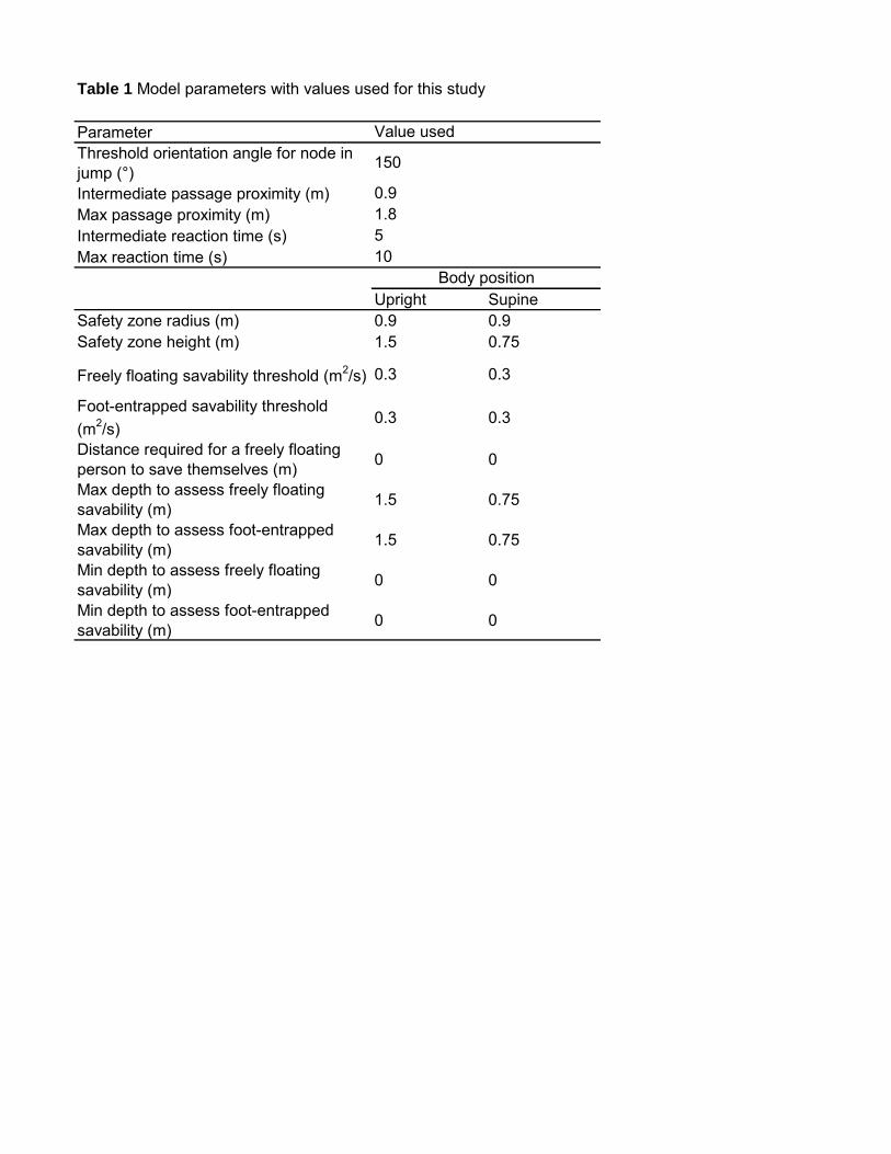
Table 1 Model parameters with values used for this study
ParameterThreshold orientation angle for node in jump (°)Intermediate passage proximity (m)Max passage proximity (m)Intermediate reaction time (s)Max reaction time (s)
Upright SupineSafety zone radius (m) 0.9 0.9Safety zone height (m) 1.5 0.75
Freely floating savability threshold (m2/s) 0.3 0.3
Foot-entrapped savability threshold (m2/s)
0.3 0.3
Distance required for a freely floating person to save themselves (m) 0 0
Max depth to assess freely floating savability (m) 1.5 0.75
Max depth to assess foot-entrapped savability (m) 1.5 0.75
Min depth to assess freely floating savability (m) 0 0
Min depth to assess foot-entrapped savability (m) 0 0
Body position
Value used
150
1.8
10
0.9
5

trauma or body entrapment. Assuming that substrate of any size and configuration had 245
the potential to cause harm under certain flow conditions, the literature on human 246
stability in a flow provided some basis for determining the flow conditions that would 247
make the substrate hazardous. A conservative assumption was also made to treat all 248
hydraulic jumps as hazardous since quantifying jump severity required complex 249
analyses beyond the scope herein. The below section introduces a concept used to 250
discriminate between safe and hazardous flow conditions for an entrained body followed 251
by sections that explain how each of the hydraulic hazard categories were defined and 252
delineated. 253
3.3.1. Savability 254
In keeping with past research concerned with human stability in a flow, this study 255
used a depth-velocity product for delineating the surface hazard types. Reported depth-256
velocity product thresholds above which adult humans lose stability from an already 257
standing or walking position range from about 0.6-2 m2/s (Abt et al. 1989; Karvonen et 258
al. 2000), though the topic at hand for this study was not a statics problem involving the 259
loss of stability, but a dynamics problem involving the potential to regain stability 260
beginning from an entrained position. For a freely floating body, savability was defined 261
as the ability for the person to overcome further transport by regaining footing in a 262
stable, standing position with head above the water surface. For an entrained body that 263
suddenly experienced foot entrapment, savability referred to the capacity to avoid 264
getting swept over and held underwater, and instead maintain a controlled upright 265
position. A rock surface could therefore be described as savable if the ambient flow 266
conditions allowed a freely floating or foot-entrapped person to save themselves by 267

achieving a stable standing position. Halting one’s forward progression while moving 268
freely with the flow or righting oneself following foot entrapment were not assumed to be 269
equivalent to maintaining upright stability from an already standing or walking position, 270
and it was reasoned that the threshold depth-velocity product below which saving was 271
possible must be lower than that for upright stability due to an entrained body’s 272
momentum. A value of 0.3 m2/s was chosen for this study to be the threshold depth-273
velocity product for savability (Table 1) with lower values corresponding to the absence 274
of hydraulic hazards given a person’s ability to save themselves and avoid harm. A 275
similar approach was taken by McCarroll et al. (2015) to determine whether a simulated 276
bather had escaped a rip current and reached a safe area by evaluating both the depth 277
and a hazard rating that uses a depth-velocity product. Co-author Pasternack has 278
extensive personal experience with savability in whitewater rivers and training beginners 279
with river safety. From his experience, the threshold value is reasonable for normal 280
recreational boaters and swimmers. It will be significantly lower for inebriated 281
inadvertent swimmers (a common presence on whitewater rivers) and higher for 282
whitewater experts. 283
It is important to note that this threshold value is only a rough estimate as this 284
study did not aim to experimentally determine this value, but instead to introduce the 285
concept of savability for which future investigation is needed. For comparison, 0.3 m2/s 286
falls within the low hazard category proposed by Cox et al. (2010) for children and 287
adults that permits stable standing and wading. These authors also suggested 0.8 m2/s 288
as the working limit for trained safety personnel. While no depth and velocity data were 289
collected to identify the threshold for regaining stability, Cox et al. (2004) posited that 290

once footing is lost, less hazardous flow conditions are required for footing to be 291
regained due to greater bodily surface area presented to the flow. It is also more 292
challenging to perform an athletic dynamic maneuver to regain footing than it is to make 293
small weight shifts to sustain existing footing, especially as one becomes more tired 294
through the exertions of avoiding hydraulic hazards. 295
3.3.2. Emergent unsavable surface hazards 296
Since no strong basis existed for discriminating among different substrate sizes 297
and arrangements in terms of the associated hazard, the full topographic surface was 298
considered in the hydraulic hazard delineation. The perimeters of emergent surfaces 299
where depth = 0 m were first identified. Next, the perimeters were delineated as 300
emergent unsavable surface hazards for a freely floating or foot-entrapped body in the 301
upright position if the adjacent water had a depth <1.5 m and a depth-velocity product 302
>0.3 m2/s (Fig. 3; Table 1). This meant that upon encountering an emergent surface 303
under these flow conditions, a person could not save themselves to regain a stable 304
standing position and was instead at risk of experiencing involuntary physical contact 305
and associated harm. 306
In areas where emergent surfaces abutted water deeper than 1.5 m, the depth 307
was considered too great to permit a 1.8 m tall person to save themselves into a 308
standing position with head above the water surface. Therefore, the depth-velocity 309
product threshold was not evaluated in these situations. It was reasoned that emergent 310
surfaces next to deep, slow water were less likely to be hazardous than those next to 311
deep, fast water. However, no threshold velocity could be discerned for what constituted 312
hazardous due to the complexities of describing the interaction of a body with a near-313
Depth > 0 m?
Depth < 1.5 m?
Deep submerged surface
Depth*velocity > 0.3 m2/s?
Submerged unsavable
surface hazard
Submerged savable surface
Adjacent to water’s edge?
High and dry surface
Yes
Yes
Yes
No
No
No
Adjacent to water with
depth < 1.5 m?
Steep emergent surface hazard
Adjacent to water with
depth*velocity > 0.3 m2/s
Emergent unsavable
surface hazard
Emergent savable surface
Yes
Yes
No
Yes
No
No
vertical rock surface, so the entirety of these surfaces was designated as steep 314
emergent surface hazards for the sake of caution. Very few of these hazards were 315
present along the study site, so they were lumped with the emergent unsavable surface 316
hazards. 317
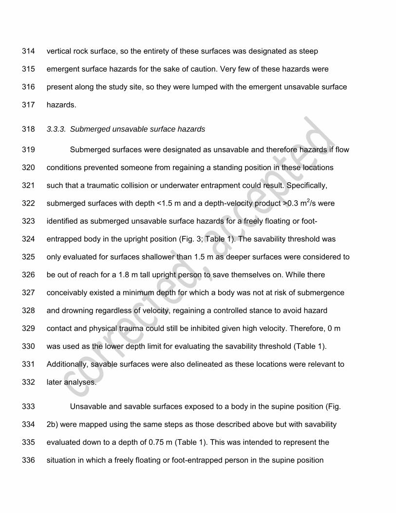
3.3.3. Submerged unsavable surface hazards 318
Submerged surfaces were designated as unsavable and therefore hazards if flow 319
conditions prevented someone from regaining a standing position in these locations 320
such that a traumatic collision or underwater entrapment could result. Specifically, 321
submerged surfaces with depth <1.5 m and a depth-velocity product >0.3 m2/s were 322
identified as submerged unsavable surface hazards for a freely floating or foot-323
entrapped body in the upright position (Fig. 3; Table 1). The savability threshold was 324
only evaluated for surfaces shallower than 1.5 m as deeper surfaces were considered to 325
be out of reach for a 1.8 m tall upright person to save themselves on. While there 326
conceivably existed a minimum depth for which a body was not at risk of submergence 327
and drowning regardless of velocity, regaining a controlled stance to avoid hazard 328
contact and physical trauma could still be inhibited given high velocity. Therefore, 0 m 329
was used as the lower depth limit for evaluating the savability threshold (Table 1). 330
Additionally, savable surfaces were also delineated as these locations were relevant to 331
later analyses. 332
Unsavable and savable surfaces exposed to a body in the supine position (Fig. 333
2b) were mapped using the same steps as those described above but with savability 334
evaluated down to a depth of 0.75 m (Table 1). This was intended to represent the 335
situation in which a freely floating or foot-entrapped person in the supine position 336
attempted to save themselves into a standing position on surfaces less than 0.75 m in 337
depth. While it was reasoned that the savability threshold for a supine body that’s either 338
freely floating or foot entrapped should still fall below the threshold for stability from an 339
already standing position, there was no strong basis for altering the threshold relative to 340
that used for the freely floating or foot-entrapped upright body. Therefore, the savability 341
threshold was maintained at 0.3 m2/s. 342
3.3.4. Hydraulic jump hazards 343
The final hazard described in this study was hydraulic jumps, which can occur 344
due to submerged surfaces and therefore account for an additional hazard associated 345
with these inundated features. The presence of aeration is a critical component of the 346
jump hazard (Valle and Pasternack 2002, 2006), as the level of aeration can be large 347
enough to prevent lifejacket buoyancy from supporting a person above the water 348
surface while also small enough to make the multiphase zone unbreathable. This study 349
only investigated the presence or absence of hydraulic jumps, as identified by the 350
transition from supercritical to subcritical flow in the 2D model output. The scheme 351
introduced in this study for locating hydraulic jumps is itself a novel tool that could be 352
used in the study of spatially explicit mountain river hydraulics. The general steps 353
involved identifying supercritical regions, isolating the perimeters of these regions, and 354
then analyzing the flow vectors at the model mesh nodes adjacent to the perimeters to 355
determine those downstream of and within a jump. The same hydraulic jumps hazards 356
were used for the supine body scenario as for the upright body, as these features were 357
assumed to be exposed to anything moving along at the water’s surface. 358
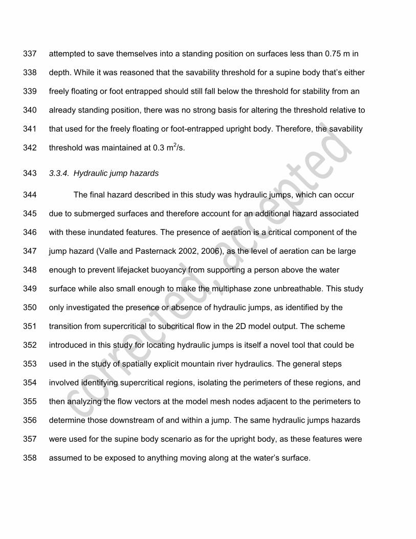
For each modeled discharge, supercritical flow regions were identified, and the 359
orientations of the flow vectors at computational mesh nodes were computed to isolate 360
the nodes immediately downstream of the supercritical flow where jumps, by definition, 361
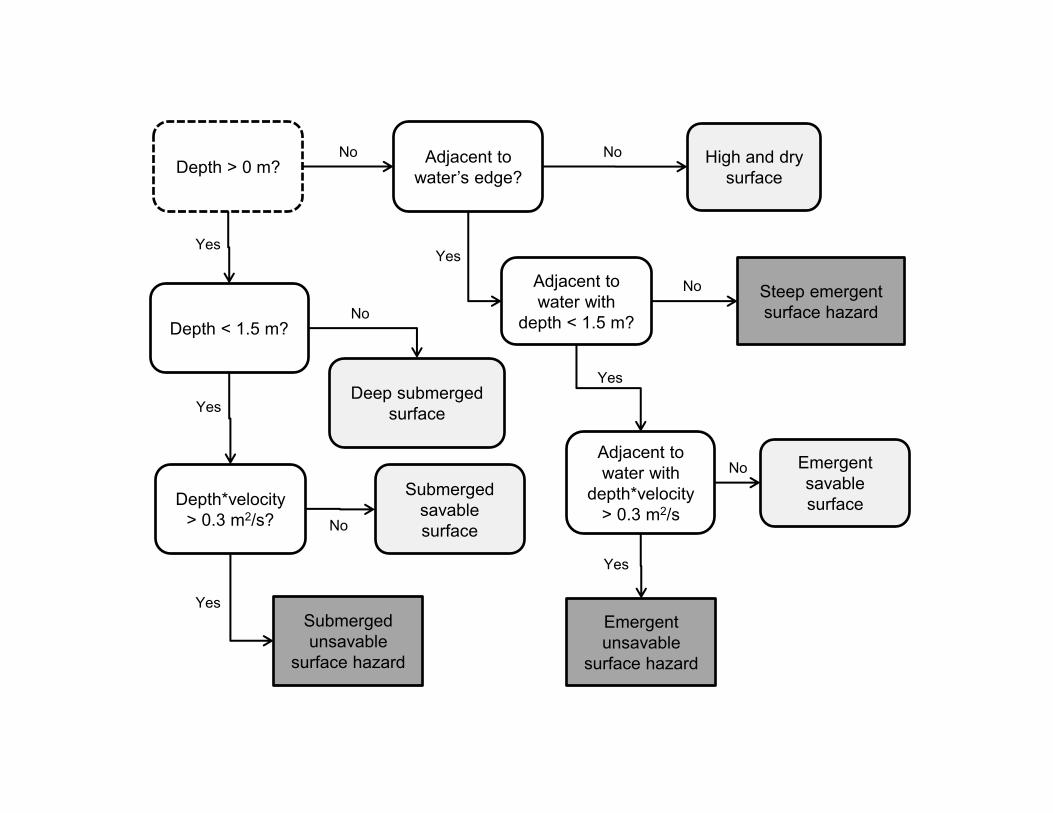
occurred. Given the angle 𝛼 of the flow vector at each mesh node (Fig. 4a) and the 362
angle 𝛽 associated with the line segment connecting that node to a point on the 363
perimeter of a supercritical flow region, the orientation angle 𝛾 of the flow vector to the 364
point was computed using the expressions below. 365
𝛽 > 𝛼: 𝛾 = |𝛽 − 180 − 𝛼| (1) 366
𝛽 < 𝛼: 𝛾 = |𝛽 + 180 − 𝛼| (2) 367
It was necessary to select a certain threshold orientation angle 𝛾 to isolate mesh 368
nodes sufficiently downstream of the supercritical flow to represent the jump location. 369
An angle of 𝛾 = 90° was tried initially, but this value erroneously included too many 370
mesh nodes on the upstream side of the supercritical flow due to raster edge effects. A 371
stricter threshold of 𝛾 = 150° was ultimately chosen such that the majority of the isolated 372
mesh nodes occurred along the appropriate downstream boundary of the supercritical 373
flow (Fig. 4b). 374
3.4. Characterizing hazard exposure 375
After delineating hazard locations, two criteria were introduced to describe the 376
instantaneous hazard exposure at any point in the river where a body might be located 377
during transit. These included passage proximity, i.e., how close a person would be 378
swept toward a hazard if they were unable to save themselves along the way, and 379
reaction time, i.e., how much time was available for the person to swim against the 380

Supercritical flow point
Flow vector
𝜶
𝜷
𝜸
(a) (b)
current to change their trajectory and avoid a close hazard encounter. A key factor in 381
evaluating hazard exposure is human motility that complicates the prediction of where a 382
body will move through a flow. Instead of trying to guess or simulate motile behavior 383
and determine the effects on hazard exposure, this study used the instantaneous 384
trajectory at all positions in the flow to map the hazard exposure and gage the need for 385
motility to avoid hazards. While hazard exposure was described using the hazard 386
locations, flow direction, and velocity magnitude, characterizing the vulnerability of 387
people to harm upon encountering a hazard was beyond the scope of this study. The 388
risk of physical trauma or drowning was represented by describing the hazard exposure 389
with the passage proximity and reaction time metrics and assuming that harm would 390
result if a hazard encounter were to occur. 391
An instantaneous trajectory of constant velocity and direction was projected from 392
the flow vector at each 2D model node, and these trajectory attributes were used to 393
quantify the two metrics as a means of characterizing the hazard exposure associated 394
with each node in the flow. This approach of projecting constant direction and velocity 395
can both over and underestimate the exposure to hazards, because at any given node 396
in the flow, the direction and velocity can either be more or less conducive to hazard 397
exposure than the conditions experienced by the body along the remainder of its actual 398
path. For example, the trajectory at one location might have a high velocity and be 399
directed at a hazard, while further down the path the velocity could decrease and the 400
direction change to a safer area, or vice versa. 401
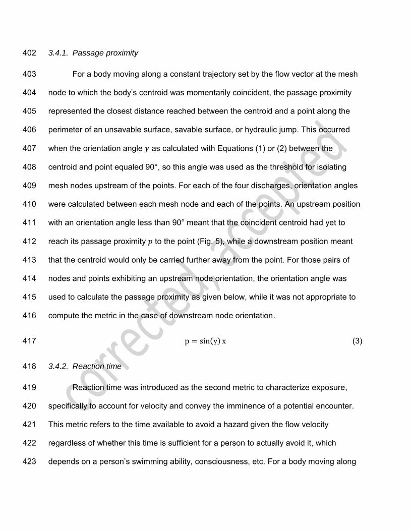
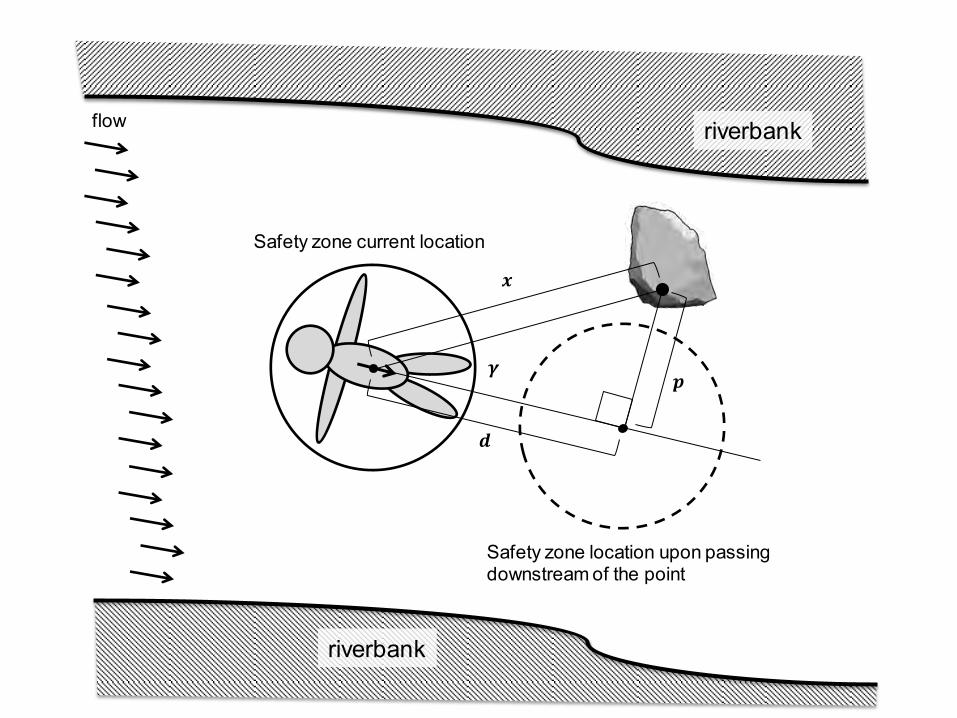
3.4.1. Passage proximity 402
For a body moving along a constant trajectory set by the flow vector at the mesh 403
node to which the body’s centroid was momentarily coincident, the passage proximity 404
represented the closest distance reached between the centroid and a point along the 405
perimeter of an unsavable surface, savable surface, or hydraulic jump. This occurred 406
when the orientation angle 𝛾 as calculated with Equations (1) or (2) between the 407
centroid and point equaled 90°, so this angle was used as the threshold for isolating 408
mesh nodes upstream of the points. For each of the four discharges, orientation angles 409
were calculated between each mesh node and each of the points. An upstream position 410
with an orientation angle less than 90° meant that the coincident centroid had yet to 411
reach its passage proximity 𝑝 to the point (Fig. 5), while a downstream position meant 412
that the centroid would only be carried further away from the point. For those pairs of 413
nodes and points exhibiting an upstream node orientation, the orientation angle was 414
used to calculate the passage proximity as given below, while it was not appropriate to 415
compute the metric in the case of downstream node orientation. 416
p = sin(γ) x (3) 417
3.4.2. Reaction time 418
Reaction time was introduced as the second metric to characterize exposure, 419
specifically to account for velocity and convey the imminence of a potential encounter. 420
This metric refers to the time available to avoid a hazard given the flow velocity 421
regardless of whether this time is sufficient for a person to actually avoid it, which 422
depends on a person’s swimming ability, consciousness, etc. For a body moving along 423
Safety zone current location
riverbank
riverbank
flow
𝒙
𝜸
𝒅
𝒑
Safety zone location upon passing downstream of the point

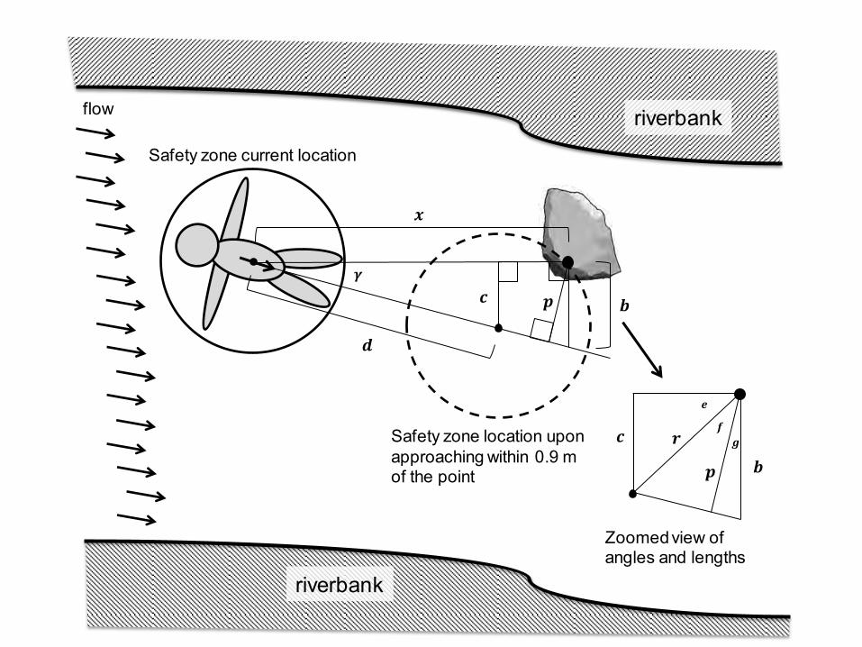
a constant trajectory at a velocity 𝑣, the reaction time computation depended on 424
whether the body’s centroid would reach within 0.9 m of an unsavable surface, savable 425
surface, or hydraulic jump point. If the centroid was not going to approach the point 426
within this distance (𝑝 > 0.9 m) as depicted in Fig. 5, then the reaction time was 427
calculated as follows with 𝑑 equal to the distance traveled by the body before passing 428
downstream of the point. 429
𝑡 =𝑑
𝑣=
cos(𝛾)𝑥
𝑣 (4) 430
Conversely, if the body’s centroid was going to approach the point within this 431
distance (𝑝 < 0.9 m), then the reaction time was computed using the below equations 432
where lengths 𝑏, 𝑐, and 𝑟 and angles 𝑒, 𝑓, and 𝑔 are defined in Fig. 6. 433
𝑏 = tan(𝛾) 𝑥 (5) 434
𝑒 = 90 − 𝑓 − 𝑔 = 90 − cos−1 (𝑝
𝑟) − cos−1 (
𝑝
𝑏) (6) 435
𝑐 = sin(𝑒) 𝑟 (7) 436
𝑡 =𝑑
𝑣=
𝑐
sin(𝛾)𝑣 (8) 437
3.4.3. Total hazard exposure 438
For each discharge, the computation of passage proximity and reaction time was 439
first made separately for emergent unsavable surfaces, submerged unsavable surfaces, 440
and hydraulic jumps to assess the exposure to each hazard category irrespective of the 441
presence of the others. Savable surfaces were included in each computation to account 442
for encounters with these safe areas that were assumed to permit saving. Only surfaces 443
riverbank
riverbank
flow
𝒙
𝜸
𝒅
𝒑 𝒃 𝒄
Safety zone current location
Safety zone location upon approaching within 0.9 m of the point
𝒑 𝒃
𝒓 𝒄
𝒆
𝒇
𝒈
Zoomed view of angles and lengths

delineated with respect to the upright body’s 1.5-m tall safety zone were used in these 444
individual hazard category computations. Next, the points for all the hazard categories 445
and savable surfaces were combined and the two metrics were again calculated to 446
characterize the total hazard exposure for the upright body. Total hazard exposure was 447
defined to be the exposure of a body to all of the three hazard types, and lastly it was 448
also calculated with the hazards delineated for the supine body such that a comparison 449
could be made with the total hazard exposure for the upright body. 450
3.4.4. Mapping hazard exposure 451
The next step was to bin the values of the two metrics for visual purposes as well 452
as to quantify the resulting areal extent of each bin. For example, how much of the river 453
segment at a given discharge exhibited the potential for encountering a hazard within 5 454
s? A baseline level of hazard exposure relevant for mapping was first established by 455
constraining the range of values for the metrics. A hazard with a sufficiently large 456
passage proximity, here defined as greater than twice the safety zone radius (1.8 m), 457
was treated as posing no threat to a body regardless of how short the reaction time was 458
(Table 1). Similarly, it was decided that hazards with reaction times larger than 10 s 459
were not a threat no matter how close the passage proximity was. These values were 460
somewhat arbitrarily chosen, but greater than 10 s was considered to be relatively safe 461
with adequate time for a person to evaluate the situation and react accordingly to the 462
flow, and over 1.8 m was judged to be plenty of distance between the hazard and 463
body’s centroid to avoid an encounter. 464
Two scenarios were considered for assigning a passage proximity and reaction 465
time to each mesh node. Where encounters were predicted to occur between the safety 466
zone and multiple hazard points based on the velocity and trajectory associated with a 467
given node, the hazard point with the shortest reaction time for an encounter 468
determined both the passage proximity and reaction time for the node (Fig. 7a). Values 469
weren’t assigned if the shortest reaction time was associated with a savable surface 470
point because these encounters were assumed to permit a person’s saving and 471
avoidance of downstream hazards. If the safety zone was predicted to near miss hazard 472
points with passage proximities between 0.9 and 1.8 m, then the point with the closest 473
passage proximity was selected to set the values of the two metrics at the node (Fig. 474
7b). 475
After assigning metric values, rasters were created for passage proximity and 476
reaction time. To classify the values of the passage proximity (PP) raster in the context 477
of the human body safety zone dimensions, a rating of two (PP2) was assigned for 478
passage proximities less than 0.9 m that corresponded to hazard encounters (Fig. 7a). 479
This rating was also given to cells upstream and within 0.9 m of a hazard point, as 480
bodies in this area were being actively pushed into the hazard. A rating of one (PP1) 481
was given for passage proximities between 0.9 and 1.8 m, which represented the near-482
miss scenario (Fig. 7b). A rating of zero (PP0) was assigned for cells with no 483
downstream hazards less than 10 s away or with passage proximities under 1.8 m. The 484
reaction times (RT) were assigned a rating of zero (RT0) for greater than 10 s or for 485
passage proximities over 1.8 m, one (RT1) for between 5 and 10 s, and two (RT2) for 486
under 5 s or if a cell was already within 0.9 m of a hazard point. For mapping the 487
exposure to submerged unsavable surface hazards, PP3 and RT3 were given to cells 488
that exhibited unsavable conditions to represent the immediate exposure of the body’s 489

Closest point to both safety zone centroids
(a)
Point with closest passage proximity Point with shortest
reaction time for a safety zone encounter
Passage proximity
(b)
Point with closest passage proximity
Passage proximity

centroid to the underlying hazard. Overlapping passage proximity and reaction time 490
rating areas were then paired to express hazard exposure with six different ratings: no 491
hazard (PP0/RT0), distant near miss (PP1/RT1), imminent near miss (PP1/RT2), distant 492
collision (PP2/RT1), imminent collision (PP2/RT2), and immediate exposure (PP3/RT3). 493
For example, Fig. 8 shows an emergent surface bound by a dashed line with 494
hypothetical paired passage proximity and reaction time ratings on the upstream side of 495
the surface. Lastly, the fraction of the wetted area occupied by each paired rating for a 496
given discharge was computed. 497
3.4.5. Longitudinal profiles 498
To provide a basic landscape context for the hazard analysis, the average 499
elevation at each longitudinal position through the river valley was computed for the 500
study segment. Next, the longitudinal distribution of total hazard exposure for each 501
discharge was determined by computing the fraction of the wetted area at each position 502
along the river that exhibited some form of exposure, e.g., PP1/RT1 or PP1/RT2, from 503
at least one of the hazards. These hazard exposure, or danger, fractions were plotted 504
as a longitudinal series in the downstream direction to reveal the locations of more and 505
less dangerous regions encountered in passage down the river. Additionally, the 506
covariance between the danger fraction distribution at 15 m3/s and that at each of the 507
higher discharges was computed and plotted as longitudinal series to reveal how 508
increasing discharge influenced the locations of dangerous regions. Lastly, the 509
cumulative distribution of the longitudinal series of danger fractions was plotted for each 510
discharge. The raw danger areas were not used to generate these cumulative 511
distributions because the danger fractions more meaningfully represented the exposure 512


of a body to danger while in transit downstream. For example, a person could enter a 513
region of the river with a large total danger area, but the channel could be very wide 514
here such that the danger fraction is low. In contrast, a region that has less danger area 515
but is also very narrow would exhibit a high danger fraction, which accurately expresses 516
a more unavoidable exposure to hazards. 517
3.4.6. Adjustable model parameters 518
At this time, the model relies on new parameters that are logical and meet 519
whitewater expert judgment, but not well constrained with high scientific certainty. Most 520
scientific theories and engineering applications are first published and used with less-521
constrained parameterizations as done here, and then future studies provide practical 522
refinements. The iterative development of the Universal Soil Loss Equation (Wischmeier 523
and Smith 1978; Renard et al. 1994) is a good example of that. Some highly popular 524
scientific parameters, such as channel roughness, remain contentious and uncertain 525
despite widespread study and application (Lane 2005; Ferguson 2010). In this case, the 526
model involved a highly hazardous phenomenon with many dangers in attempting field-527
scale parameter calibration at the study site under the discharges of interest. In light of 528
this uncertainty, the assumptions behind the current model parameter values are 529
reported to convey the uncertainty of the results and highlight opportunities for 530
refinement. 531
Experiments in controlled flume settings can inform adjustments to the model 532
parameters listed in Table 1. The concept of savability was used to describe the 533
capacity for a person to regain a controlled upright stance with head above the water 534
surface starting from either a freely floating or foot-entrapped upright or supine position. 535
A single threshold was used to account for all four of these situations, but the ability to 536
save oneself in each scenario may actually correspond to different thresholds. 537
Additionally, a depth-velocity product might not be sufficient for capturing the savability 538
in the two freely floating situations as saving could also hinge on the distance over 539
which one is exposed to flow that does not exceed a certain threshold. Experimental 540
analysis could determine, for example, that a distance of 3 m is required for an adult 541
moving along with a current exhibiting a depth-velocity product of 0.2 m2/s to save 542
themselves. In this study, it was assumed that instantaneous saving was possible upon 543
encountering water with a depth-velocity product below 0.3 m2/s. The minimum and 544
maximum depth for assessing savability could also be clarified as a function of subject 545
height. Lastly, the threshold orientation angle used to isolate mesh nodes downstream 546
of supercritical flow could be field validated by mapping the locations of hydraulic jumps 547
and comparing these to the node locations. 548
In contrast, other parameter values may be adjusted a priori depending on the 549
application. These include the safety zone dimensions, which are tied to the height of 550
the human subjects of interest as well as the maximum passage proximity and reaction 551
time used to map and analyze the hazard exposure. 552
3.4.7. Hazard model validation 553
At this time only limited validation of the hydraulic hazard model theorized and 554
applied to the validated 2D model was performed, which involved a visual comparison 555
of the predicted and observed hydraulic jump hazard locations. In addition, co-author 556
Pasternack used his expert whitewater experience and training in whitewater safety to 557
qualitatively evaluate whether the model results were reasonable at individual rapids in 558
the SYR as he has kayaked and swam portions of the river at different discharges. 559
Whole branches of science involve exploration of nature using back-of-the-envelope 560
calculations and numerical models with no chance for validation presently, such as 561
Earth’s interior dynamism, landscape evolution modeling over thousands to millions of 562
years, geomorphic modeling of other planets, and various solar and galactic dynamics. 563
Natural hazards present a unique situation, because they involve the Earth’s extreme 564
dynamics, with infrequent periodicity, large size, flashiness, and deadly hazards. A good 565
case in point of a model development arc is the SHALSTAB model for predicting maps 566
of shallow landslide hazards, whose equations and results were published with no 567
validation (Dietrich et al. 1992), leading to widespread usage in hazard management. 568
The authors published a field study with some model validation nine years later (Dietrich 569
et al. 2001). Even now, many flood hazard studies lack hydrodynamic validation data 570
(e.g., Chen and Liu 2016). Nevertheless, planners must design evacuation schemes 571
and management plans on the basis of whatever they can, so having the best analysis 572
possible is warranted regardless of the ideal of model validation. 573
If a sponsor were to fund a model validation effort to test the results of this model 574
in a future study, then the ideal approach would be to deploy human analogs into a 575
flood and use large-scale particle image velocimetry to measure passage proximity and 576
reaction time associated with each hydraulic hazard, and then compare those to model 577
predictions. Whitewater rivers with roads that run along them, like the one used in this 578
study or the North Fork of the Payette River in Idaho are excellent locations for testing. 579
Human test dummies replicate the dimensions, weight proportions and articulation of 580
the human body, while pig carcasses are widely regarded as the best organic analog of 581
humans. These could be positioned upstream either manually or using the robotic river 582
truss (Pasternack et al., 2006a). Pole-mounted cameras or tethered kite-blimps would 583
be deployed to capture the velocity field of the ambient flow and track the motion of the 584
test subject. These data would be used to measure passage proximities and compute 585
reaction times, ideally for a wide range of flows. Although this is not difficult to envision, 586
it would be costly and difficult to schedule in light of flood unpredictability. Since the 587
underlying topographic and hydraulic data for this study was collected in 2009, 588
California has experienced a historic drought and only a few days of flooding have 589
occurred between then and when this hazard study was completed. 590
One aspect of the model that was more amenable to validation was the 591
delineation of the hydraulic jump hazards since these could be safely photographed in 592
the field and compared to the locations mapped using the approach developed in this 593
study. For example, jump hazards were photographed during a flow of 4.4 m3/s at the 594
Langs Crossing gage and were visually compared to the locations of jumps delineated 595
with 2D model results for this flow. Figure 9 shows the confluence of Canyon Creek with 596
the South Yuba River where hydraulic jumps are associated with several steps. 597
Features such as the steps in the photo were represented well in the DEM, and the 598
corresponding flow acceleration was therefore reproduced closely by the 2D model. In 599
contrast, other locations with smaller-scale causes of flow acceleration, such as 600
individual boulders or shaped bedrock protrusions, were not as well captured in the 601
DEM and 1-m resolution computational mesh, so the occurrence of supercritical flow 602
was often underpredicted by the 2D model in these locations, leading to an 603
underpredicted occurrence of jump hazards. The eddy viscosity coefficient also affected 604

(a)
(b)
the extent of supercritical flow predicted by the 2D model as it determined the efficiency 605
of momentum transfer. 606
4. Results 607
4.1. Hazard exposure maps 608
Mapping the hazard exposure permitted visual assessment of how the algorithms 609
captured the interaction of the hazards with the hydraulics. Hazard exposure maps for 610
the full study segment at 31 m3/s for each hazard type as well as the total of all hazards 611
are provided in Online Resources 2-5. Fig. 10 illustrates the results for four different 612
scenarios for hazard encounters in the study segment, with the first two maps (Fig. 10a, 613
b) involving emergent unsavable surfaces, hydraulic jumps for the third map, and 614
submerged unsavable surfaces for the bottom map. While present in each of the maps, 615
the submerged unsavable surfaces (PP3/RT3) were only displayed in Fig. 10d. 616
Excluding the non-hazard area (PP0/RT0), the remaining PP/RT rating areas in each 617
map composed the danger zones for the mapped hazards. The danger zones and 618
component areas exhibited different shapes and sizes depending on the flow direction, 619
velocity magnitude, depth, and hazard configuration. In Fig. 10a, the danger zone 620
showed a flared upstream end due to convergent flow with more vectors oriented 621
directly to the hazard to produce either a near miss or an encounter. The danger zone in 622
Fig. 10b had a tapered tip because of flow that diverged from the hazard here and 623
expanded out toward the right bank, but bank narrowing just downstream converged 624
flow toward the hazard and enlarged the danger zone midsection. 625


In addition to flow direction, velocity magnitude and depth influenced the danger 626
zones. The hazard points associated with two jumps are shown in Fig. 10c, with the 627
lower jump exhibiting a danger zone with a tip skewed away from the left bank. The 628
boundary between PP2/RT2 and PP2/RT1 also showed this skew which resulted from a 629
gradient in velocity laterally across the danger zone with slower velocities closer to the 630
left bank. The danger zone of the upper jump showed comparatively little skew due to 631
more uniform velocities across the width of the zone. However, the longitudinal extents 632
of the danger zone areas containing RT2 versus RT1 differed due to a velocity gradient 633
along the length of the zone. Flow accelerated toward the jump such that more of the 634
danger zone was within 5 s of a jump point, whereas the absence of a gradient would 635
yield equal longitudinal extents of areas within 5 and 10 s of a hazard. Depth was 636
relevant to the danger zones because the depth-velocity product determined the 637
distribution of submerged savable surfaces that suppressed the extent of the danger 638
zones. The left side of the lower danger zone in Fig. 10c lacked PP1/RT2 and PP1/RT1 639
area because the adjacent submerged savable surface was already within a body’s 640
safety zone here for which saving was assumed to be possible. 641
The hazard configuration specifically affected the danger zone component areas. 642
The jumps present within the segment consisted of laterally distributed clusters of 643
hazard points such as those displayed in Fig. 10c. As a result, the danger zone areas 644
with PP2 were much more extensive than those with PP1 as hazard encounters rather 645
than near misses were more likely. Longitudinally distributed clusters of hazard points 646
like those shown in Fig. 10d favored areas with RT2 and not RT1, since flow was 647
consistently within 5 s of an encounter or near miss with a hazard. The PP2/RT1 and 648
PP1/RT1 area in the lower left and right corners of Fig. 10d was associated with 649
downstream submerged unsavable surface hazards not visible in the panel. 650
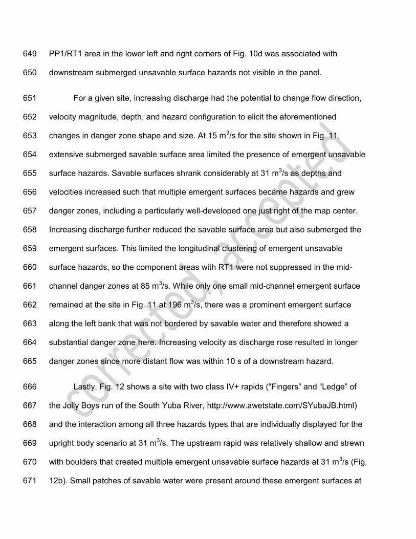
For a given site, increasing discharge had the potential to change flow direction, 651
velocity magnitude, depth, and hazard configuration to elicit the aforementioned 652
changes in danger zone shape and size. At 15 m3/s for the site shown in Fig. 11, 653
extensive submerged savable surface area limited the presence of emergent unsavable 654
surface hazards. Savable surfaces shrank considerably at 31 m3/s as depths and 655
velocities increased such that multiple emergent surfaces became hazards and grew 656
danger zones, including a particularly well-developed one just right of the map center. 657
Increasing discharge further reduced the savable surface area but also submerged the 658
emergent surfaces. This limited the longitudinal clustering of emergent unsavable 659
surface hazards, so the component areas with RT1 were not suppressed in the mid-660
channel danger zones at 85 m3/s. While only one small mid-channel emergent surface 661
remained at the site in Fig. 11 at 196 m3/s, there was a prominent emergent surface 662
along the left bank that was not bordered by savable water and therefore showed a 663
substantial danger zone here. Increasing velocity as discharge rose resulted in longer 664
danger zones since more distant flow was within 10 s of a downstream hazard. 665
Lastly, Fig. 12 shows a site with two class IV+ rapids (“Fingers” and “Ledge” of 666
the Jolly Boys run of the South Yuba River, http://www.awetstate.com/SYubaJB.html) 667
and the interaction among all three hazards types that are individually displayed for the 668
upright body scenario at 31 m3/s. The upstream rapid was relatively shallow and strewn 669
with boulders that created multiple emergent unsavable surface hazards at 31 m3/s (Fig. 670
12b). Small patches of savable water were present around these emergent surfaces at 671

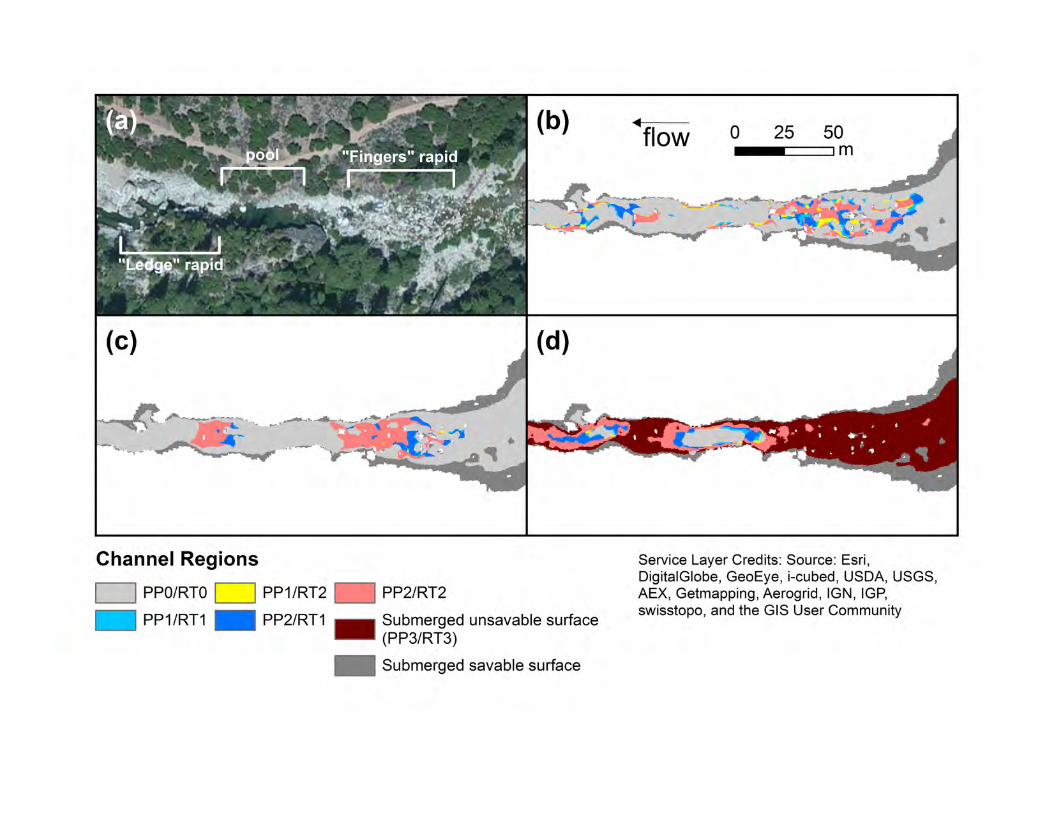
this discharge that limited the extent of the danger zones in some places. These 672
boulders also accelerated flow to form jump hazards here (Fig. 12c). Due to depths <1.5 673
m and high velocities, nearly all of the submerged surfaces here were unsavable (Fig. 674
12d). Just downstream was a pool adjacent to steep bedrock walls (Fig. 12a) where 675
slow velocities and large depths produced few hazards at 31 m3/s. The next rapid 676
occurred immediately downstream where the higher bed elevation and the narrow 677
bedrock walls converged flow to form a large jump hazard. Only a couple mid-channel 678
surfaces were emergent here, and the surfaces that were <1.5 m deep were mostly 679
unsavable. 680
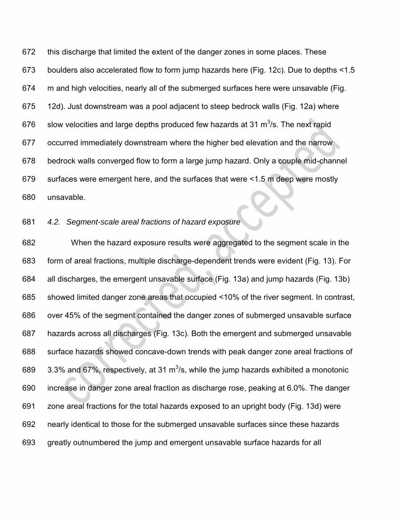
4.2. Segment-scale areal fractions of hazard exposure 681
When the hazard exposure results were aggregated to the segment scale in the 682
form of areal fractions, multiple discharge-dependent trends were evident (Fig. 13). For 683
all discharges, the emergent unsavable surface (Fig. 13a) and jump hazards (Fig. 13b) 684
showed limited danger zone areas that occupied <10% of the river segment. In contrast, 685
over 45% of the segment contained the danger zones of submerged unsavable surface 686
hazards across all discharges (Fig. 13c). Both the emergent and submerged unsavable 687
surface hazards showed concave-down trends with peak danger zone areal fractions of 688
3.3% and 67%, respectively, at 31 m3/s, while the jump hazards exhibited a monotonic 689
increase in danger zone areal fraction as discharge rose, peaking at 6.0%. The danger 690
zone areal fractions for the total hazards exposed to an upright body (Fig. 13d) were 691
nearly identical to those for the submerged unsavable surfaces since these hazards 692
greatly outnumbered the jump and emergent unsavable surface hazards for all 693

0.9
0.92
0.94
0.96
0.98
1
15 31 85 196 15 31 85 196
0.2
0.4
0.6
0.8
1
15 31 85 196 15 31 85 196 15 31 85 196
PP3/RT3PP2/RT2PP2/RT1PP1/RT2PP1/RT1PP0/RT0
Are
al fr
actio
n of
seg
men
t
Discharge (m3/s)
(b)(a)
(c) (d) (e)

discharges. The total hazard areal fractions for the supine body position (Fig. 13e) were 694
substantially lower than these for the upright position. 695
The component fractions of the danger zones also changed across discharges, 696
i.e., the fractions of the danger zone areas occupied by the paired passage proximity 697
and reaction time ratings. For emergent unsavable surface and jump hazards, 698
increasing discharge coincided with an overall increase in each component area except 699
for clear declines in PP2/RT2 (Table 2). For submerged unsavable surface hazards and 700
the total hazards for both body positions, the PP3/RT3 area declined significantly as 701
discharge increased, while the remaining component areas showed overall increases. 702
PP3/RT3 was particularly dominant within the danger zones at 15 and 31 m3/s for 703
submerged unsavable surface hazards and total hazards for the upright position. 704
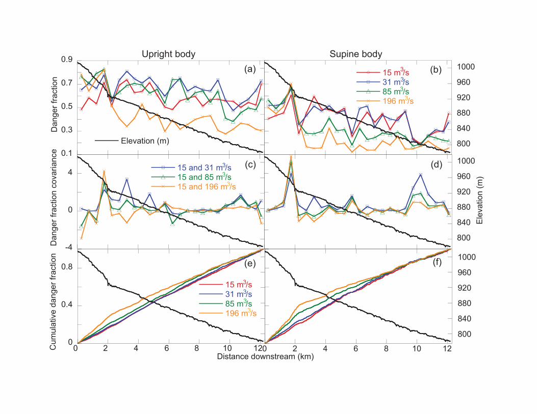
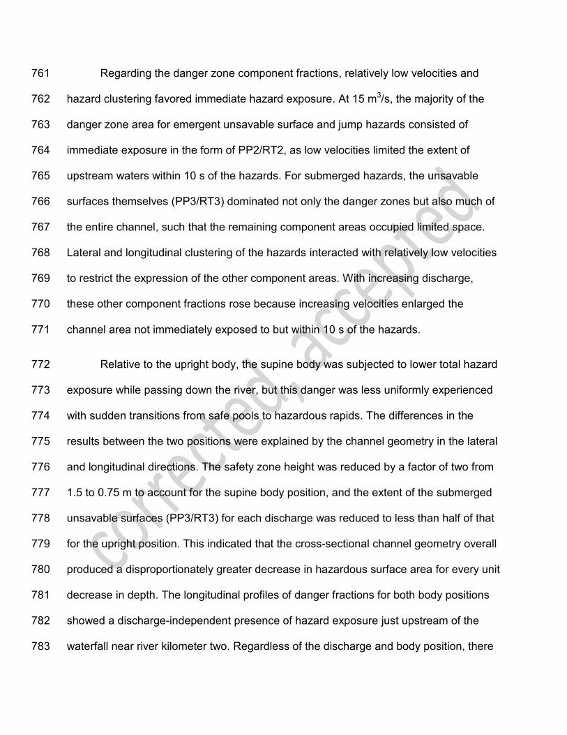
4.3. Longitudinal profiles 705
The profile of elevation along the valley centerline indicated the presence of two 706
dominant slopes across the study segment, with the steeper upstream region ending 707
abruptly at a large waterfall around river kilometer two (Fig. 14). Due to the local 708
variability in hazard occurrence and the associated danger zone extents, the 709
longitudinal distributions of the polygon danger fractions exhibited considerable noise. 710
The average danger fractions within 0.5-km windows along the study segment were 711
instead plotted to help visualize the trends (Fig. 14a, b). For both the upright (Fig. 14a) 712
and supine (Fig. 14b) body positions, high danger fractions for all discharges occurred 713
just upstream of the waterfall at river kilometer two with sharp drops in the danger 714
fractions immediately downstream. For the upright position, the danger fractions at 15, 715
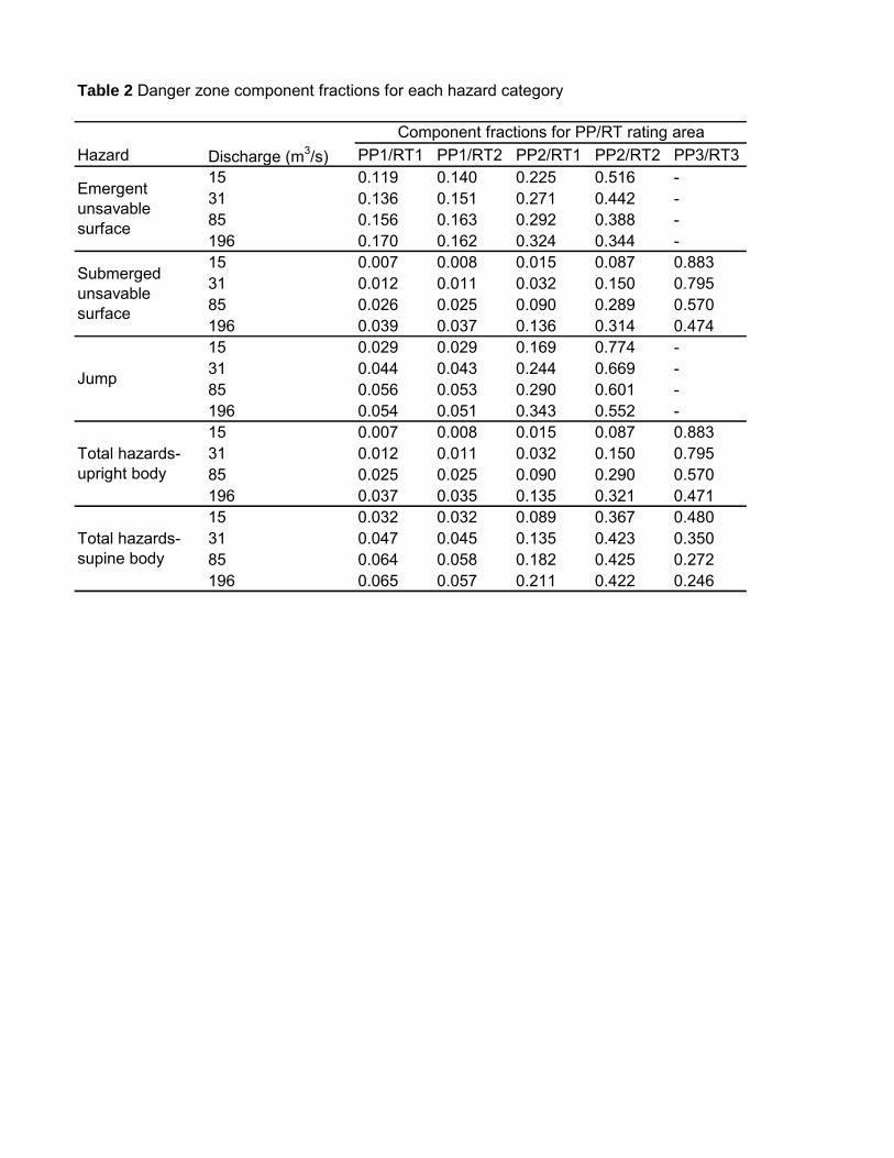
Table 2 Danger zone component fractions for each hazard category
Hazard Discharge (m3/s) PP1/RT1 PP1/RT2 PP2/RT1 PP2/RT2 PP3/RT315 0.119 0.140 0.225 0.516 -31 0.136 0.151 0.271 0.442 -85 0.156 0.163 0.292 0.388 -196 0.170 0.162 0.324 0.344 -15 0.007 0.008 0.015 0.087 0.88331 0.012 0.011 0.032 0.150 0.79585 0.026 0.025 0.090 0.289 0.570196 0.039 0.037 0.136 0.314 0.47415 0.029 0.029 0.169 0.774 -31 0.044 0.043 0.244 0.669 -85 0.056 0.053 0.290 0.601 -196 0.054 0.051 0.343 0.552 -15 0.007 0.008 0.015 0.087 0.88331 0.012 0.011 0.032 0.150 0.79585 0.025 0.025 0.090 0.290 0.570196 0.037 0.035 0.135 0.321 0.47115 0.032 0.032 0.089 0.367 0.48031 0.047 0.045 0.135 0.423 0.35085 0.064 0.058 0.182 0.425 0.272196 0.065 0.057 0.211 0.422 0.246
Total hazards-supine body
Component fractions for PP/RT rating area
Emergent unsavable surface
Submerged unsavable surface
Jump
Total hazards-upright body
0.1
0.3
0.5
0.7
0.9
Elevation (m) 800
840
880
920
960
100015 m /s31 m /s85 m /s196 m /s
-4
0
4 15 and 31 m /s15 and 85 m /s15 and 196 m /s
0
0.4
0.8
15 m /s31 m /s85 m /s196 m /s
0 2 4 6 8 10 12
800
840
880
920
960
1000
800
840
880
920
960
1000
0 2 4 6 8 10 12
Dan
ger f
ract
ion
Cum
ulat
ive
dang
er fr
actio
nD
ange
r fra
ctio
n co
varia
nce
Ele
vatio
n (m
)
Distance downstream (km)
(a) (b)
(c) (d)
(e) (f)
Upright body ine body
3
33
3
3
3
3
3
33
3

31, and 85 m3/s rose rapidly downstream of this point of low danger, while for the 716
supine position, only the 15 and 31 m3/s danger fractions showed a rapid increase here. 717
The covariance distributions revealed the presence of both discharge-dependent 718
and discharge-independent danger (Fig. 14c, d). A positive value of covariance at any 719
location in the profile meant that danger, or lack thereof, was discharge independent 720
between the two flows (i.e., between 15 m3/s and a higher flow), while negative values 721
indicated that the danger changed between the flows. Danger fraction covariance 722
showed more positive values for the supine (Fig. 14d) than the upright (Fig. 14c) 723
position, and both positions showed peaks for each distribution just upstream of the 724
waterfall. The cumulative distributions of danger fractions for all four discharges under 725
the supine body scenario (Fig. 14f) deviated more from a uniform distribution of danger 726
than those for the upright position (Fig. 14e), and the less smooth curves for the supine 727
position indicated greater local accumulations of danger fractions. Within the first two 728
river kilometers, the 196 m3/s distribution for both body positions showed the most 729
pronounced accumulation of danger fractions with progressively reduced accumulations 730
in order of decreasing discharge. 731
5. Discussion 732
5.1. Understanding hazard exposure across the study segment 733
In aggregating the hazard exposure results to the segment scale, there existed a 734
balance at 31 m3/s between the extent of surfaces that were exposed to a body in either 735
position and the extent of unsavable water that made these surfaces hazardous. The 736
overall decline in the danger zone areal fractions for emergent unsavable surface 737

hazards over the discharge series indicated that mid-channel emergent surfaces were 738
overwhelmingly inundated at the highest discharge. While emergent surface hazards 739
arose along the banks where unsavable water became more extensive with increasing 740
discharge, the danger zone areal fractions declined in part because these bank 741
locations constituted one-sided hazard exposure. Mid-channel hazards could be 742
encountered by a body from either side of the hazards, and the associated danger 743
zones were therefore larger than those for hazards along the banks. The decline was 744
additionally attributed to the decreasing wetted-perimeter-to-wetted-area ratio with rising 745
discharge as hazard recruitment along the banks did not counter the expansion in 746
channel area. The submerged unsavable surface hazards also declined overall with 747
discharge, as once the mid-channel surfaces were submerged too deeply, only narrow 748
bands of these submerged hazards were present along the banks. The danger zone 749
areal fractions for both surface hazards did increase from 15 to 31 m3/s before 750
declining, as the factors responsible for the occurrence of these hazards were optimized 751
at this intermediate discharge. Velocities overall continued to increase beyond 31 m3/s, 752
and the extent of unsavable water expanded. However, the mid-channel surfaces were 753
inundated too deeply at higher discharges to be hazards. In contrast, the inundation of 754
surfaces created additional flow-accelerating features, e.g., boulders over which water 755
spilled at high velocity, that expanded the extent of not only unsavable water but also 756
supercritical flow and jump hazards. These conditions were prevalent enough to 757
compensate for the drowning out of features that accelerated flow at lower discharges, 758
such that the danger zone areal fractions for jump hazards monotonically rose with 759
discharge. 760
Regarding the danger zone component fractions, relatively low velocities and 761
hazard clustering favored immediate hazard exposure. At 15 m3/s, the majority of the 762
danger zone area for emergent unsavable surface and jump hazards consisted of 763
immediate exposure in the form of PP2/RT2, as low velocities limited the extent of 764
upstream waters within 10 s of the hazards. For submerged hazards, the unsavable 765
surfaces themselves (PP3/RT3) dominated not only the danger zones but also much of 766
the entire channel, such that the remaining component areas occupied limited space. 767
Lateral and longitudinal clustering of the hazards interacted with relatively low velocities 768
to restrict the expression of the other component areas. With increasing discharge, 769
these other component fractions rose because increasing velocities enlarged the 770
channel area not immediately exposed to but within 10 s of the hazards. 771
Relative to the upright body, the supine body was subjected to lower total hazard 772
exposure while passing down the river, but this danger was less uniformly experienced 773
with sudden transitions from safe pools to hazardous rapids. The differences in the 774
results between the two positions were explained by the channel geometry in the lateral 775
and longitudinal directions. The safety zone height was reduced by a factor of two from 776
1.5 to 0.75 m to account for the supine body position, and the extent of the submerged 777
unsavable surfaces (PP3/RT3) for each discharge was reduced to less than half of that 778
for the upright position. This indicated that the cross-sectional channel geometry overall 779
produced a disproportionately greater decrease in hazardous surface area for every unit 780
decrease in depth. The longitudinal profiles of danger fractions for both body positions 781
showed a discharge-independent presence of hazard exposure just upstream of the 782
waterfall near river kilometer two. Regardless of the discharge and body position, there 783
were always features here that generated hazards and yielded a peak in the danger 784
fraction profile. The discharge independence of the danger upstream of the waterfall 785
was confirmed by the positive covariance values for each distribution at this location 786
along the river. The 85 m3/s profile for the upright position increased between river 787
kilometers two and 3.75 but remained low for the supine position, as this region of the 788
segment was plane bed with few features to create hazards under high discharges and 789
a supine body position. Deep pools, such as the one present around river kilometer 790
5.75, had slow velocities and drowned-out surfaces that produced discharge-791
independent safety as supported by low danger fractions and positive covariance for 792
each distribution here. The negative covariance between 15 and 196 m3/s for the 793
upright body revealed that channel locations switched from dangerous to safe (river 794
kilometers 3.25 and 12.1) or vice versa (river kilometer 0.25) for this position between 795
these two discharges. The region that became more dangerous was explained by a 796
secondary channel thread that was relatively calm at 15 m3/s but became much more 797
hazardous at 196 m3/s. For both body positions, increasing discharge corresponded to 798
an upstream loading of the danger fraction cumulative distributions as hazards were 799
largely drowned out beyond river kilometer two. Relative to the cumulative distributions 800
for the upright body, the more abrupt increases in the distributions for the supine body 801
indicated a greater sensitivity to the dichotomous step-pool channel geometry that was 802
present along much of the segment. 803
5.2. Model implications 804
This study has broached the topic of how to mechanistically characterize the 805
exposure of people to hazards upon entrainment in a whitewater river. Flood-related 806
deaths are not linked exclusively to whether or not people have been swept away. A 807
survey of people affected by the Bangladesh cyclone of 1991 found that 112 out of 285 808
people (39%) who were carried away by the storm surge died (Bern et al., 1993). The 809
hazard delineation procedure used herein offers a foundation for identifying the 810
locations of hazards for which refinements can be adopted depending on the setting. 811
For example, the automated mapping of unsavable surfaces in an urban flood 812
environment can be paired with the manual delineation of specific features that are of 813
particular concern for causing physical trauma and body entrapment. However, the 814
model developed in this study does not account for changes to the landscape as a 815
result of flood flows that may alter the hydraulics and the distribution of hazards, such 816
as the mobilization of debris in an urban setting (Chanson et al., 2014). The methods 817
introduced in this study also do not address other urban flood hazards including 818
drowning within a vehicle that’s driven into floodwaters. 819
Given the complexity of predicting where a volitional, inertial body would move 820
within a flow field, multiple simplifications were made that permitted a substantive first 821
step for this line of research. Instantaneous hazard exposure was quantified for any 822
point in the flow where a body could be present, though Lagrangian particle tracking 823
would be the next logical step to more rigorously assess the hazard exposure of a body 824
moving along a path through the flow under a variety of different scenarios. This 825
includes someone who has fallen out of their raft within a rapid or someone who has 826
lost stability while evacuating a residence and swept down a flooded street. This could 827
also help determine the connectivity of safe flow regions present along a river or flooded 828
neighborhood through which people may be carried with relatively low exposure to 829
hazards. 830
6. Conclusion 831
This study presented a new, analytical approach to characterizing the exposure 832
of people to hazards within a flow. LiDAR and two-dimensional model results for a 833
segment of the South Yuba River offered a unique opportunity to delineate hazards and 834
mechanistically describe the exposure of an entrained body to these features for a 835
whitewater river setting. Passage proximity and reaction time were introduced as 836
metrics derived from the velocity magnitude and direction to express a body’s hazard 837
exposure. Increasing discharge produced concave-down trends in the body’s exposure 838
to emergent and submerged unsavable surface hazards, while a monotonic increase 839
occurred for exposure to jump hazards. The total hazard exposure faced by a body 840
moving down the river in the upright position was greater than that for a supine body, 841
although the supine body experienced a less uniform exposure to hazards including 842
abrupt encounters with dangerous channel regions. Further investigation is needed for 843
the concept of savability given its importance to quantifying hazard exposure, such that 844
the model may be applied to other dangerous flow settings like urban floods. 845
Acknowledgements 846
No external grant was provided directly for this work. Indirect support was 847
received from the USDA National Institute of Food and Agriculture, Hatch project 848
number #CA-D-LAW-7034-H. Precursor data were collected for different purposes with 849
an award from the Instream Flow Assessment Program of the Public Interest Energy 850

Research Program of the California Energy Commission. The Instream Flow 851
Assessment Program was administered by the Center of Aquatic Biology and 852
Aquaculture of the University of California, Davis. This project involved a large 853
collaborative effort that was only possible by gracious contributions of effort and 854
resources by many people, including relicensing stakeholders, their consultants, our 855
paid project staff, and UC Davis student volunteers. Helpful reviews and feedback of the 856
final technical report with the 2D model and other precursor study components leading 857
up the work herein were provided by Professor Allen James (University of South 858
Carolina), Dudley Reiser (R2 Resource Consultants, Inc), Michael Barclay (HDR/DTA), 859
Thomas Studley (PG&E), and Dr. Joshua Wyrick (Lafayette College). Lastly, Daniel 860
Brasuell provided assistance in locating the rapids present along the study segment. 861
References 862
Abt SR, Wittler RJ, Taylor A, Love DJ (1989) Human stability in a high flood hazard. 863
Water Resour Bull 25(4):881-890. doi: 10.1111/j.1752-1688.1989.tb05404.x 864
Belknap L (1998) Upgrading the American version of the International Scale of River 865
Difficulty. American Whitewater. 866
https://www.americanwhitewater.org/content/Wiki/safety:introratings?. 867
Bern C, Sniezek J, Mathbor GM, Siddiqi MS, Ronsmans C, Chowdhury AMR, 868
Choudhury AE, Islam K, Bennish M, Noji E, Glass RI (1993) Risk Factors for 869
Mortality in the Bangladesh Cyclone of 1991. Bulletin of the WHO 71:73-78. 870
Chanson H, Brown R, McIntosh D (2014) Human body stability in floodwaters: the 2011 871
flood in Brisbane CBD. 5th IAHR International Symposium on Hydraulic 872
Structures 1-9, The University of Queensland 873
Chen WB, Liu WC (2016) Assessment of storm surge inundation and potential hazard 874
maps for the southern coast of Taiwan. Nat Hazards 82(1): 591-616 doi: 875
10.1007/s11069-016-2199-y 876
Cox RJ, Yee M, Ball JE (2004) Safety of people in flooded streets and floodways, 877
National Conference on Hydraulics in Water Engineering, Engineers Australia 878
Cox RJ, Shand TD, Blacka MJ (2010) Australian Rainfall and Runoff revision project 10: 879
Appropriate safety criteria for People, Engineers Australia 880
Dietrich WE, Bellugi D, Real de Asua R (2001) Validation of the Shallow Landslide 881
Model, SHALSTAB, for forest management. In: Wigmosta MS, Burges SJ (eds) 882
Land Use and Watersheds: Human influence on hydrology and geomorphology 883
in urban and forest areas, vol Water Science and Application 2. American 884
Geophysical Union, pp 195-227 885
Dietrich WE, Wilson CJ, Montgomery DR, McKean J, Bauer R (1992) Erosion 886
Thresholds and Land Surface-Morphology Geology 20:675-679Dolan R, Howard 887
A, Trimble D (1978) Structural control of the rapids and pools of the Colorado 888
River in the Grand Canyon. Science 202(4368): 629-631 doi: 889
10.1126/science.202.4368.629 890
Ferguson R (2010) Time to abandon the Manning equation? Earth Surf Proc Land 891
35:1873-1876 doi: 10.1002/esp.2091 892
Foster DN, Cox RJ (1973) Stability of children on roads used as floodways. University of 893
New South Wales Water Research Laboratory Technical Report 73(13) 894

Gard M (2003) Flow-habitat relationships for spring-run Chinook salmon spawning in 895
Butte Creek. Energy Planning and Instream Flow Branch Butte Creek 2D 896
Modeling Final Report, U.S. Fish and Wildlife Service 897
Gonzalez RL, Pasternack GB (2015) Re-envisioning cross-sectional hydraulic geometry 898
as spatially explicit hydraulic topography. Geomorphology 246:394–406 doi: 899
10.1016/j.geomorph.2015.06.024 900
Graf WL (1979) Rapids in canyon rivers. J Geol 533-551 901
Grant GE, Swanson FJ, Wolman MG (1990) Pattern and origin of stepped-bed 902
morphology in high-gradient streams, Western Cascades, Oregon. Geol Soc Am 903
Bull 102(3):340-352 doi: 10.1130/0016-904
7606(1990)102<0340:PAOOSB>2.3.CO;2 905
Harrison LR, Keller EA (2007) Modeling forced pool–riffle hydraulics in a boulder-bed 906
stream, southern California. Geomorphology 83(3):232-248 doi: 907
10.1016/j.geomorph.2006.02.024 908
Hauer C, Mandlburger G, Habersack H (2009) Hydraulically related hydromorphological 909
units: description based on a new conceptual mesohabitat evaluation model 910
(MEM) using LiDAR data as geometric input. River Res Appl 25:29-47 911
doi:10.1002/rra.1083 912
Hilldale RC, Raff D (2008) Assessing the ability of airborne LiDAR to map river 913
bathymetry. Earth Surf Proc Land 33(5):773-783 doi: 10.1002/esp.1575 914
Jonkman SN (2005) Global perspectives on loss of human life caused by floods. Nat 915
Hazards 34(2):151-175 doi: 10.1007/s11069-004-8891-3 916
Jonkman SN, Kelman I (2005) An analysis of the causes and circumstances of flood 917
disaster deaths. Disasters 29(1):75-97 doi: 10.1111/j.0361-3666.2005.00275.x 918
Jonkman SN, Penning‐Rowsell E (2008) Human Instability in Flood Flows. J Am Water 919
Resour As 44(5):1208-1218 doi: 10.1111/j.1752-1688.2008.00217.x 920
Karvonen RA, Hepojoki A, Huhta HK, Louhio A (2000) The use of physical models in 921
dam-break analysis. RESCDAM Final Report, Helsinki University of Technology, 922
Helsinki, Finland 923
Keller RJ, Mitsch B (1993) Safety aspects of the design of roadways as floodways. 924
Urban Water Research Association of Australia 925
Kieffer SW (1985) The 1983 hydraulic jump in Crystal Rapid: Implications for river-926
running and geomorphic evolution in the Grand Canyon. J Geol 385-406 927
Lai YG (2008) SRH-2D version 2: Theory and User’s Manual. U.S. Department of the 928
Interior, Bureau of Reclamation 929
Lane SN (2005) Roughness – time for a re-evaluation? Earth Surf Proc Land 30:251-930
253 doi: 10.1002/esp.1208 931
Lane SN, Chandler JH (2003) Editorial: the generation of high quality topographic data 932
for hydrology and geomorphology: new data sources, new applications and new 933
problems. Earth Surf Proc Land 28(3):229-230 doi: 10.1002/esp.479 934
Leopold LB (1969) The rapids and the pools—Grand Canyon. U.S. Geological Survey 935
Professional Paper 669:131-145 936
Lind N, Hartford D, Assaf H (2004) Hydrodynamic Models of Human Instability in a 937
Flood. J Am Water Resour As 40(1):89-96 doi: 10.1111/j.1752-938
1688.2004.tb01012.x 939
McCarroll RJ, Castelle B, Brander RW, Scott T (2015) Modelling rip current flow and 940
bather escape strategies across a transverse bar and rip channel morphology. 941
Geomorphology 246:502-518 doi: 10.1016/j.geomorph.2015.06.041 942
McKean JA, Isaak DJ, Wright CW (2008) Geomorphic controls on salmon nesting 943
patterns described by a new, narrow-beam terrestrial-aquatic lidar. Front Ecol 944
Environ 6(3):125–130 doi: 10.1890/070109 945
Milanesi L, Pilotti M, Ranzi R (2015) A conceptual model of people's vulnerability to 946
floods. Water Resour Res 51(1):182-197 doi: 10.1002/2014WR016172 947
Muste M, Kim D, Merwade V (2012) Modern Digital Instruments and Techniques for 948
Hydrodynamic and Morphologic Characterization of River Channels. In: Church 949
M et al. (ed) Gravel-Bed Rivers: Processes, Tools, Environments, John Wiley & 950
Sons, Ltd., Chichester, UK pp 315-341 951
Pasternack GB, Valle BL, Paige D, Shaw M (2006a) Portable apparatus and method for 952
measuring hydraulic features in rivers and streams. United States Patent Office, 953
Patent #7062962 954
Pasternack GB, Ellis CR, Leier KA, Valle BL, Marr JD (2006b) Convergent hydraulics at 955
horseshoe steps in bedrock rivers. Geomorphology 82(1):126-145 956
Pasternack GB, Senter AE (2011) 21st Century instream flow assessment framework 957
for mountain streams. California Energy Commission, PIER, CEC‐500-2013-059 958
Peng SH (2012) 1D and 2D Numerical Modeling for Solving Dam-Break Flow Problems 959
Using Finite Volume Method. J Appl Math 2012 960
http://dx.doi.org/10.1155/2012/489269. 961
Penning-Rowsell EC, Floyd P, Ramsbottom D, Surendran S (2005) Estimating injury 962
and loss of life in floods: A deterministic framework. Nat Hazards 36:43-64 doi: 963
10.1007/s11069-004-4538-7 964
Reinfelds I, Lincoln-Smith M, Haeusler T, Ryan D, Growns I (2010) Hydraulic 965
assessment of environmental flow regimes to facilitate fish passage through 966
natural riffles: Shoalhaven river below Tallowa Dam, New South Wales, 967
Australia. River Res Appl 26(5):589–604 doi: 10.1002/rra.1262. 968
Renard KG, Foster GR, Yoder DC, McCool DK (1994) RUSLE Revisited - Status, 969
Questions, Answers, and the Future J Soil Water Conserv 49:213-220 970
Russo B, Gómez M, Macchione F (2013) Pedestrian hazard criteria for flooded urban 971
areas. Nat Hazards 69(1):251-265 doi: 10.1007/s11069-013-0702-2 972
Strom MA, Pasternack GB, Wyrick JR (2016) Reenvisioning velocity reversal as a 973
diversity of hydraulic patch behaviours. Hydrol Process 30(13):2348-2365 doi: 974
10.1002/hyp.10797 975
Takahashi S, Endoh K, Muro ZI (1992) Experimental study on people’s safety against 976
overtopping waves on breakwaters. Report on the Port and Harbour Institute 977
34(4):4-31 978
Valle BL, Pasternack GB (2002) TDR Measurements of Hydraulic Jump Aeration in the 979
South Fork of the American River, California. Geomorphology 42(1):153-165 980
doi:10.1016/S0169-555X(01)00083-6 981
Valle BL, Pasternack GB (2006) Air concentrations of submerged and unsubmerged 982
hydraulic jumps in a bedrock step-pool channel. J Geophys Res 111(F3):1-12 983
doi: 10.1029/2004JF000140 984

Vilming S (1998) The development of the multibeam echosounder: An historical 985
account. J Acoust Soc Am 103(2935) http://dx.doi.org/10.1121/1.422177 986
Webb RH, Pringle PT, Reneau SL, Rink GR (1988) Monument Creek debris flow, 1984: 987
Implications for formation of rapids on the Colorado River in Grand Canyon 988
National Park. Geology 16(1):50-54 doi: 10.1130/0091-7613(1988)989
016<0050:MCDFIF>2.3.CO;2 990
Webb RH, Pringle PT, Rink GR (1989) Debris flows from tributaries of the Colorado 991
River, Grand Canyon National Park, Arizona. U.S. Geological Survey 992
Professional Paper 87-118 993
Western U.S. Historical Summaries by State, Annual Precipitation Averages and 994
Extremes. Western Regional Climate Center. 995
http://www.wrcc.dri.edu/htmlfiles/ca/ca.ppt.ext.html. Accessed 23 October 2010 996
Wischmeier WH, Smith DD (1978) Predicting rainfall erosion losses: a guide to 997
conservation planning. Agriculture Handbook 537, United States Department of 998
Agriculture, Washington, DC 999
Wyrick JR, Pasternack GB (2014) Geospatial organization of fluvial landforms in a 1000
gravel-cobble river: beyond the riffle-pool couplet. Geomorphology 213:48-65 doi: 1001
10.1016/j.geomorph.2013.12.040 1002
Xia J, Falconer RA, Wang Y, Xiao X (2014) New criterion for the stability of a human 1003
body in floodwaters. J Hydraul Res 52(1):93-104 doi: 1004
10.1080/00221686.2013.875073 1005

Ying X, Wang SS (2010) Evaluation of 2D shallow-water model for spillway flow with a 1006
complex geometry. J Hydraul Res 48(2):265–268 doi: 1007
10.1080/00221681003704178 1008
1009
Figure Captions 1010
Fig. 1 Study segment location in California and within the Yuba River watershed 1011
Fig. 2 Human body safety zones for the (a) upright and (b) supine positions 1012
Fig. 3 Decision tree for the surface hazard delineation that begins with the dashed-line 1013 rounded box in the upper left and ends with hazardous surfaces in the dark-shaded 1014 squared boxes and safe surfaces in the light-shaded rounded boxes 1015
Fig. 4 (a) Orientation γ of the flow vector to the supercritical flow point given the vector 1016 angle 𝛼 and the angle 𝛽 of the line connecting the vector to the point; (b) a site 1017 demonstrating the delineated jump hazard points 1018
Fig. 5 Scenario in which the body’s centroid does not approach within 0.9 m of a 1019 hazardous surface, savable surface, or hydraulic jump point 1020
Fig. 6 Scenario in which the body’s centroid does approach within 0.9 m of a hazardous 1021 surface, savable surface, or hydraulic jump point 1022
Fig. 7 The appropriate hazard points, marked as squares, for setting the reaction time 1023 rating at a mesh node given (a) a PP2 rating and (b) a PP1 rating 1024
Fig. 8 Kite-blimp imagery of the SYR with the dashed-line perimeter of an emergent 1025 surface plus the associated hypothetical paired rating areas 1026
Fig. 9 (a) Photo looking upstream at hydraulic jumps at the confluence of Canyon Creek 1027 (left) and the South Yuba River (right); (b) predicted locations of supercritical flow and 1028 hydraulic jumps for the discharge in (a) (aerial imagery shows a lower baseflow) 1029
Fig. 10 Four scenarios with different danger zone shapes and sizes and flow vectors 1030 scaled independently for each panel to the velocity magnitude 1031
Fig. 11 A site at four different discharges with danger zones mapped for emergent 1032 unsavable surface hazards only 1033
Fig. 12 (a) Aerial imagery of two rapids with (b) emergent unsavable surface hazards, 1034 (c) jump hazards, and (d) submerged unsavable surface hazards for an entrained 1035 upright body at 31 m3/s 1036
Fig. 13 Segment-scale areal fractions of exposure to (a) emergent unsavable surface 1037 hazards, (b) jump hazards, (c) submerged unsavable surface hazards, (d) total hazards 1038 for the upright body, and (e) total hazards for the supine body 1039
Fig. 14 Longitudinal profiles of valley centerline elevation and danger fractions 1040 averaged within 0.5 km windows for (a) the upright and (b) supine bodies; longitudinal 1041 profiles of danger fraction covariance averaged within 0.5 km windows for (c) the upright 1042 and (d) supine bodies; longitudinal profiles of cumulative danger fractions for (e) the 1043 upright and (f) supine bodies 1044

Supplemental materials
Topographic mapping data
For the SYR, the entire 12.2 km study segment was surveyed in the summer of
2009. Airborne LiDAR data of the terrestrial river corridor as well as bedrock outcrops
and emergent boulders in the wetted base flow channel averaged 1 point per 0.74 m.
Because the SYR had many large emergent boulders within the wetted area at base
flow, the LiDAR survey was able to map many of them with multiple points; then a novel
data-processing and object identification workflow was used to delineate each boulder
as an object (Pasternack and Senter 2011). In this way, 34,113 individual boulders were
explicitly resolved in the DEM–an important and unique aspect of this study in order to
address hydraulic hazards. Ground-based wadeable channel surveys were done using
a Leica TPS1200 robotic total station, a Topcon GTS-603 total station, and Trimble
5700 RTK GPS. Survey point density was ~1 point every 5 m on a rough grid and 1
point every 1 m along the thalweg. Bathymetric data was collected in pools using a
pontoon-mounted Sonarmite echosounder coupled to a Trimble 5700 RTK GPS. This
rig was floated laterally and longitudinally along pool cross-sections spaced ~5 m apart,
and with data collected on a 5 s time interval. Combining these data collection methods,
the segment-averaged topographic point density was 38-39 points per 100 m2 both
within and beyond the 0.283 m3/s base flow domain.
Data collected using different observational methods were compared (i.e., every
method against every other method) where they overlapped to assess uncertainty, with
full details reported in Pasternack and Senter (2011). Each survey method involved
internal performance tests, such as backsight checks, GPS root mean square values,
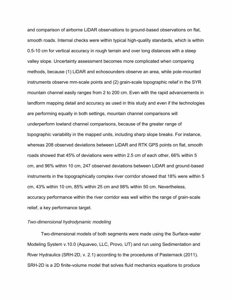
and comparison of airborne LiDAR observations to ground-based observations on flat,
smooth roads. Internal checks were within typical high-quality standards, which is within
0.5-10 cm for vertical accuracy in rough terrain and over long distances with a steep
valley slope. Uncertainty assessment becomes more complicated when comparing
methods, because (1) LiDAR and echosounders observe an area, while pole-mounted
instruments observe mm-scale points and (2) grain-scale topographic relief in the SYR
mountain channel easily ranges from 2 to 200 cm. Even with the rapid advancements in
landform mapping detail and accuracy as used in this study and even if the technologies
are performing equally in both settings, mountain channel comparisons will
underperform lowland channel comparisons, because of the greater range of
topographic variability in the mapped units, including sharp slope breaks. For instance,
whereas 208 observed deviations between LiDAR and RTK GPS points on flat, smooth
roads showed that 45% of deviations were within 2.5 cm of each other, 66% within 5
cm, and 96% within 10 cm, 247 observed deviations between LiDAR and ground-based
instruments in the topographically complex river corridor showed that 18% were within 5
cm, 43% within 10 cm, 85% within 25 cm and 98% within 50 cm. Nevertheless,
accuracy performance within the river corridor was well within the range of grain-scale
relief, a key performance target.
Two-dimensional hydrodynamic modeling
Two-dimensional models of both segments were made using the Surface-water
Modeling System v.10.0 (Aquaveo, LLC, Provo, UT) and run using Sedimentation and
River Hydraulics (SRH-2D, v. 2.1) according to the procedures of Pasternack (2011).
SRH-2D is a 2D finite-volume model that solves fluid mechanics equations to produce
an estimate for depth and velocity at each computational node (Lai 2008). SRH-2D
implements a hybrid structured-unstructured mesh that can use both quadrilateral and
triangular elements of any size allowing for mesh detail comparable to any finite-
element model.
Although this study focuses on four modeled flows associated with the spring
snowmelt hydrological regime with respect to investigating hydraulic hazards, flows
were actually modeled over three orders of magnitude for three hydrologic seasons
(dry, wet, and snowmelt) for additional hydraulic, geomorphic, and ecological analyses
(Pasternack and Senter 2011). Input discharge was obtained from USGS gaging
stations on the South Yuba River at Lang’s Crossing (#11414250) and on Canyon
Creek below Bowman (#11416500). The South Yuba River has substantial ungaged
accretionary flows, so a thorough hydrological analysis was completed (Pasternack and
Senter, 2011) yielding regression relations to estimate accretionary flows from the major
ungaged tributaries for three different hydrological seasons (wet, dry, and snowmelt). A
stage-discharge relation was made between the total gaged inflows (SYR at Lang’s
Crossing plus Canyon Creek below Bowman) and observed water surface elevations at
the exit of the study segment for total inflows ranging from 0.424 to 200.65 m3/s. The
time lag between inflow gage values and outflow WSE values was estimated for both
gages and accounted for in the stage-discharge relation. For the remote outlet of the
upstream computational mesh there was no appropriate location for a stage recorder.
That model’s downstream WSE was set to equal the simulated WSE at the entrance to
the downstream computational mesh for that flow simulation.

To simulate hydrodynamics over the discharge range investigated with
reasonable computational efficiency, it is beneficial to create different computational
meshes that span key inundation extents and divide the length of a river segment into
two or more linked sections. For the SYR, two inundation extents (< ~30 m3/s and <
~200 m3/s) and two longitudinal sections (study entrance to upstream of confluence with
Canyon Creek, and upstream of Canyon Creek to study terminus) were used, all with 1-
m internodal spacing. The downstream low and high flow meshes had 331,593 and
467,272 elements, respectively. The upstream low and high flow meshes had 284,461
and 396,615 elements, respectively. For each flow-regime simulation, the results from
the two reaches were merged to create a single point file for evaluation in GIS using the
output processing workflows explained in Pasternack (2011).
Roughness associated with resolved bedform topography (e.g., alluvial bars,
partially to fully emergent boulders and boulder clusters, and bedrock outcrops) was
explicitly represented in the detailed channel DEM and the 1 m resolution computational
mesh. Given the heterogeneity of bed material, bedrock, and vegetation as well as the
presence of all such features impacting hydraulic roughness across a wide range of
flows, unresolved bed roughness was parameterized using a spatially and flow
independent Manning’s n value of 0.1. This value was confirmed through depth and
velocity validation as well as sensitivity analysis.
Extensive model validation was performed for model simulations over two orders
of magnitude of flow ranges (~0.62 to 26.5 m3/s combined flow from the two inflow
gages). Mass conservation between specified input flow and computed output flows for
simulations of observed conditions was within 1%, except for the lowest flow simulation

of the upstream mesh. That one run had a loss of 1.9%, which was considered
reasonable given the extreme complexity of the channel topography and uncertainty in
accretionary flows at the lowest discharge (which is well below the base flow discharge
used for MU mapping in this study). WSE performance was tested by comparing 17,198
pairs of model predictions against LiDAR observations throughout the two meshes at
base flow for a mean signed deviation of -2.8 cm. Performance was best where the
water surface was flat and smooth and worst in steep sites with waves, but data from all
areas were aggregated to obtain the unsigned statistical distribution of error. For
unsigned deviations, 34% of test points were within 5 cm vertical, 51% within 10 cm,
and 91% within 25 cm. Surface velocity magnitude was measured at 273 locations and
compared to depth-averaged model predictions using the method of Barker (2011),
yielding a good predicted versus observed r2 of 0.61. Further analysis revealed that r2
was 0.8 when velocities were limited to those in pools or transitional areas between
pools and other morphological units. It was 0.5-0.64 on planar surfaces in the channel
and in the floodway. The only unsatisfactory performance occurred in steep sites with
waves where r2 was 0.06. Median unsigned velocity magnitude error was 28% for all
observations, but also varied depending on morphological unit type from 21-36%.
Interestingly, steep sites with waves had a reasonable median unsigned error of 25%.
Overall, the SYR 2D model met all common standards of 2D model performance in
aggregate, but some care was needed in the use of values at the steepest sites where
the horizontal flow assumption was violated. Even though SRH-2D is assumed to be
stable for simulating extremely steep reaches, model performance in predicting precise
velocities appears to suffer in such areas. Prediction accuracy only matters to the extent
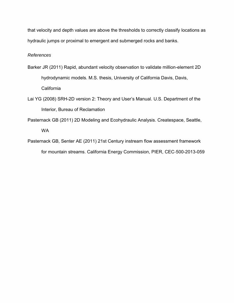
that velocity and depth values are above the thresholds to correctly classify locations as
hydraulic jumps or proximal to emergent and submerged rocks and banks.
References
Barker JR (2011) Rapid, abundant velocity observation to validate million-element 2D
hydrodynamic models. M.S. thesis, University of California Davis, Davis,
California
Lai YG (2008) SRH-2D version 2: Theory and User’s Manual. U.S. Department of the
Interior, Bureau of Reclamation
Pasternack GB (2011) 2D Modeling and Ecohydraulic Analysis. Createspace, Seattle,
WA
Pasternack GB, Senter AE (2011) 21st Century instream flow assessment framework
for mountain streams. California Energy Commission, PIER, CEC‐500-2013-059

Channel RegionsPP0/RT0PP1/RT1
PP1/RT2PP2/RT1
PP2/RT2Submerged savable surface
0 100 20050 m
Ü
SYR Emergent Unsavable Surface Hazards at 31 m3/s, p. 1

Channel RegionsPP0/RT0PP1/RT1
PP1/RT2PP2/RT1
PP2/RT2Submerged savable surface
0 100 20050 m
Ü
SYR Emergent Unsavable Surface Hazards at 31 m3/s, p. 2
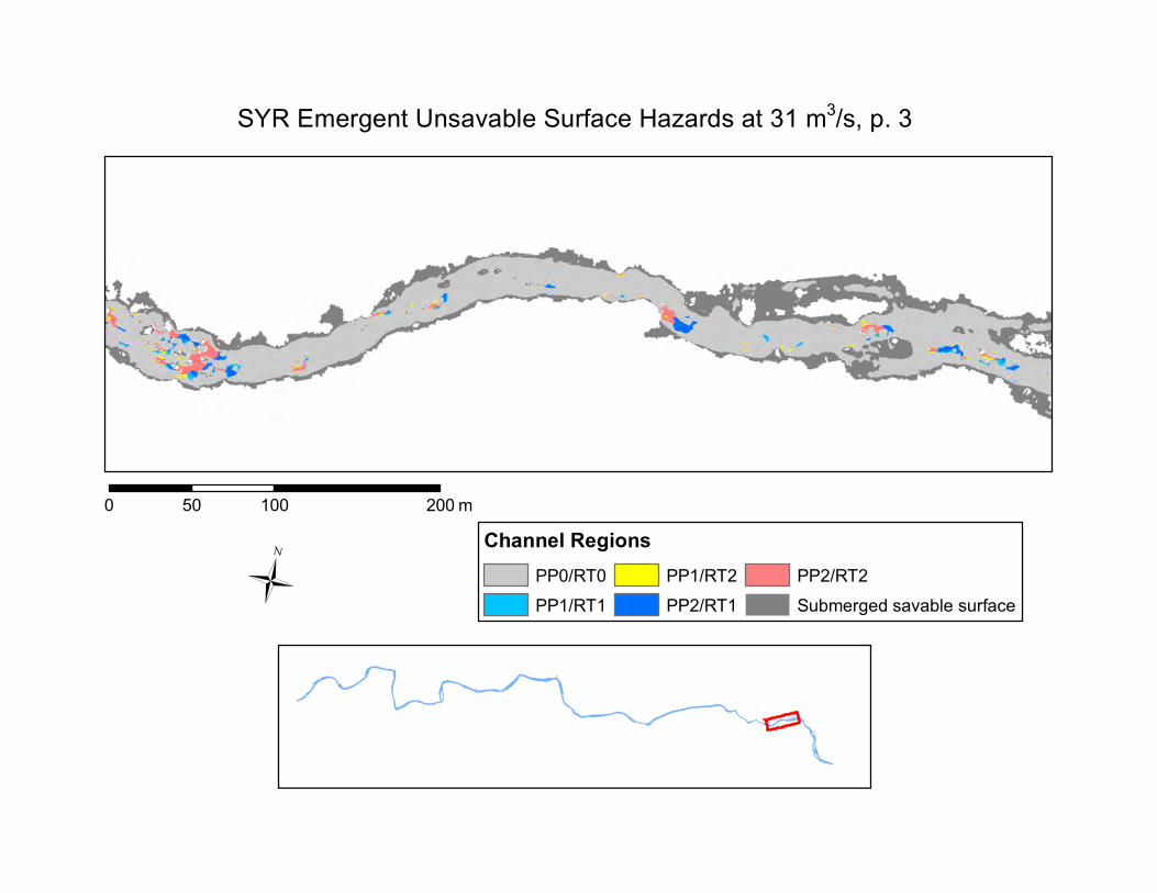
Channel RegionsPP0/RT0PP1/RT1
PP1/RT2PP2/RT1
PP2/RT2Submerged savable surface
0 100 20050 m
Ü
SYR Emergent Unsavable Surface Hazards at 31 m3/s, p. 3

Channel RegionsPP0/RT0PP1/RT1
PP1/RT2PP2/RT1
PP2/RT2Submerged savable surface
0 100 20050 m
Ü
SYR Emergent Unsavable Surface Hazards at 31 m3/s, p. 4
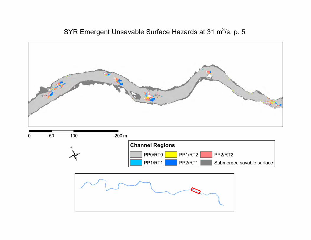
Channel RegionsPP0/RT0PP1/RT1
PP1/RT2PP2/RT1
PP2/RT2Submerged savable surface
0 100 20050 m
Ü
SYR Emergent Unsavable Surface Hazards at 31 m3/s, p. 5

Channel RegionsPP0/RT0PP1/RT1
PP1/RT2PP2/RT1
PP2/RT2Submerged savable surface
0 100 20050 m
Ü
SYR Emergent Unsavable Surface Hazards at 31 m3/s, p. 6

Channel RegionsPP0/RT0PP1/RT1
PP1/RT2PP2/RT1
PP2/RT2Submerged savable surface
0 100 20050 m
Ü
SYR Emergent Unsavable Surface Hazards at 31 m3/s, p. 7

Channel RegionsPP0/RT0PP1/RT1
PP1/RT2PP2/RT1
PP2/RT2Submerged savable surface
0 100 20050 m
Ü
SYR Emergent Unsavable Surface Hazards at 31 m3/s, p. 8
Channel RegionsPP0/RT0PP1/RT1
PP1/RT2PP2/RT1
PP2/RT2Submerged savable surface
0 100 20050 m
Ü
SYR Emergent Unsavable Surface Hazards at 31 m3/s, p. 9

Channel RegionsPP0/RT0PP1/RT1
PP1/RT2PP2/RT1
PP2/RT2Submerged savable surface
0 100 20050 m
Ü
SYR Emergent Unsavable Surface Hazards at 31 m3/s, p. 10

Channel RegionsPP0/RT0PP1/RT1
PP1/RT2PP2/RT1
PP2/RT2Submerged savable surface
0 100 20050 m
Ü
SYR Emergent Unsavable Surface Hazards at 31 m3/s, p. 11
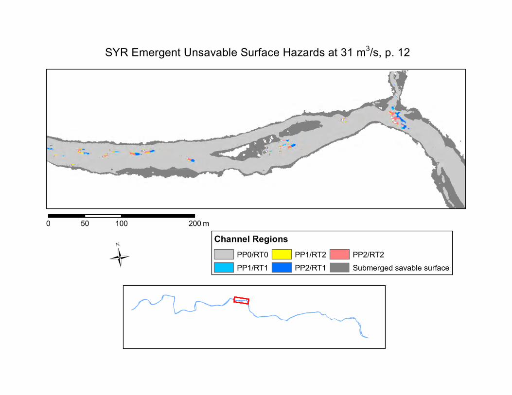
Channel RegionsPP0/RT0PP1/RT1
PP1/RT2PP2/RT1
PP2/RT2Submerged savable surface
0 100 20050 m
Ü
SYR Emergent Unsavable Surface Hazards at 31 m3/s, p. 12
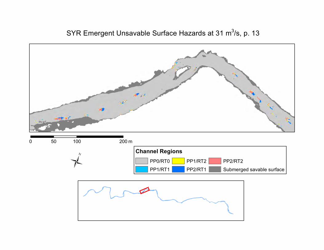
Channel RegionsPP0/RT0PP1/RT1
PP1/RT2PP2/RT1
PP2/RT2Submerged savable surface
0 100 20050 m
Ü
SYR Emergent Unsavable Surface Hazards at 31 m3/s, p. 13

Channel RegionsPP0/RT0PP1/RT1
PP1/RT2PP2/RT1
PP2/RT2Submerged savable surface
0 100 20050 m
Ü
SYR Emergent Unsavable Surface Hazards at 31 m3/s, p. 14

Channel RegionsPP0/RT0PP1/RT1
PP1/RT2PP2/RT1
PP2/RT2Submerged savable surface
0 100 20050 m
Ü
SYR Emergent Unsavable Surface Hazards at 31 m3/s, p. 15
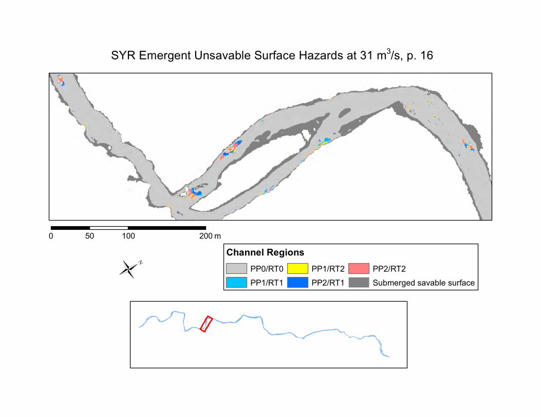
Channel RegionsPP0/RT0PP1/RT1
PP1/RT2PP2/RT1
PP2/RT2Submerged savable surface
0 100 20050 m
Ü
SYR Emergent Unsavable Surface Hazards at 31 m3/s, p. 16
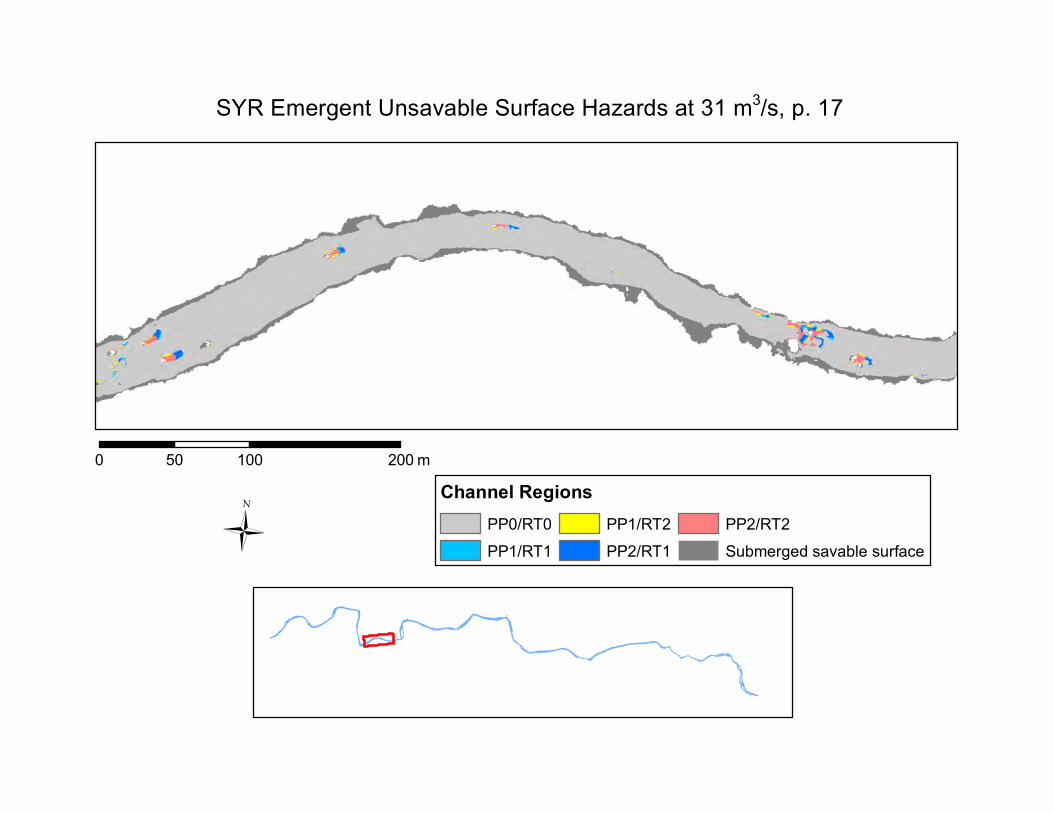
Channel RegionsPP0/RT0PP1/RT1
PP1/RT2PP2/RT1
PP2/RT2Submerged savable surface
0 100 20050 m
Ü
SYR Emergent Unsavable Surface Hazards at 31 m3/s, p. 17
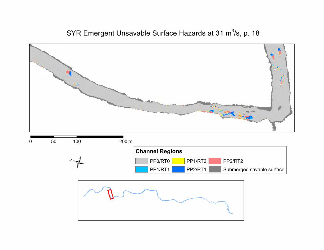
Channel RegionsPP0/RT0PP1/RT1
PP1/RT2PP2/RT1
PP2/RT2Submerged savable surface
0 100 20050 m
Ü
SYR Emergent Unsavable Surface Hazards at 31 m3/s, p. 18
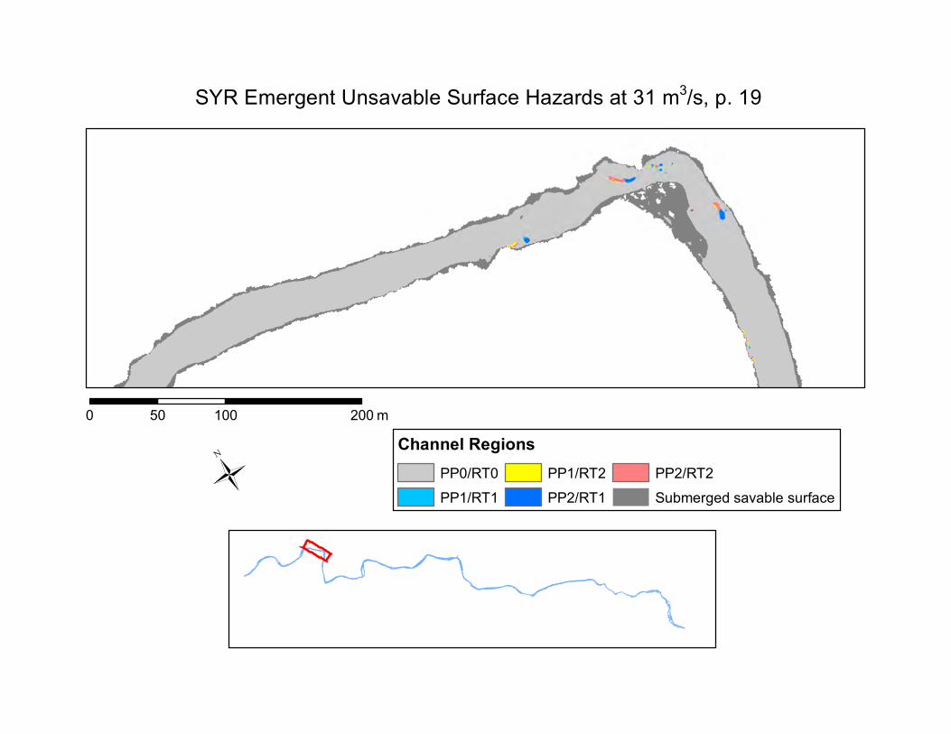
Channel RegionsPP0/RT0PP1/RT1
PP1/RT2PP2/RT1
PP2/RT2Submerged savable surface
0 100 20050 m
Ü
SYR Emergent Unsavable Surface Hazards at 31 m3/s, p. 19
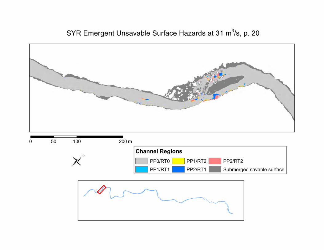
Channel RegionsPP0/RT0PP1/RT1
PP1/RT2PP2/RT1
PP2/RT2Submerged savable surface
0 100 20050 m
Ü
SYR Emergent Unsavable Surface Hazards at 31 m3/s, p. 20
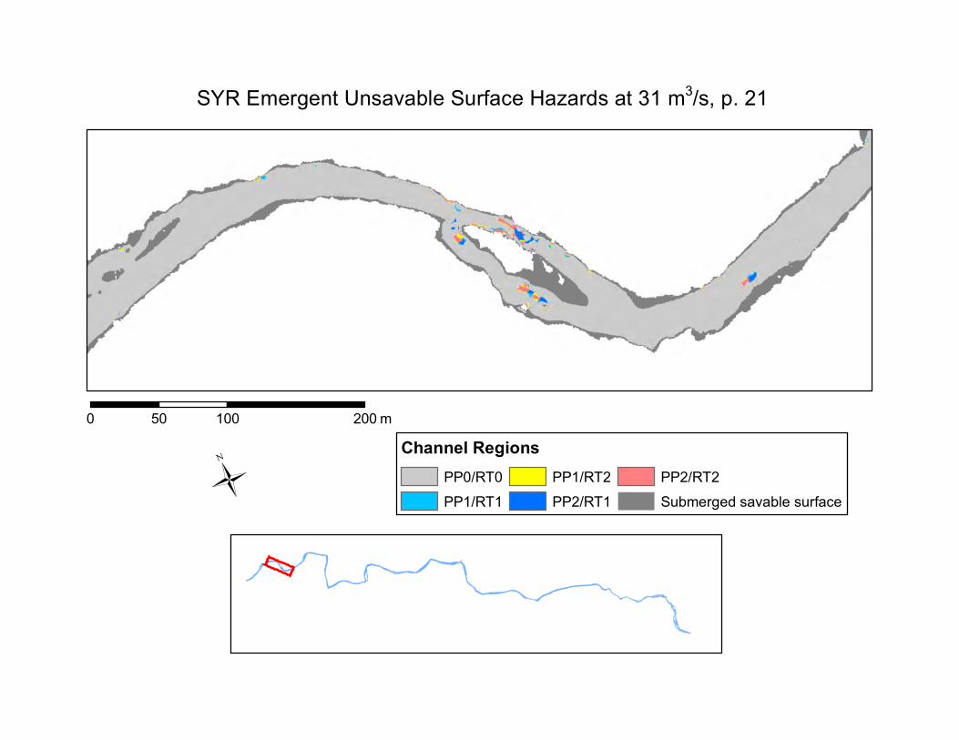
Channel RegionsPP0/RT0PP1/RT1
PP1/RT2PP2/RT1
PP2/RT2Submerged savable surface
0 100 20050 m
Ü
SYR Emergent Unsavable Surface Hazards at 31 m3/s, p. 21

Channel RegionsPP0/RT0PP1/RT1
PP1/RT2PP2/RT1
PP2/RT2Submerged savable surface
0 100 20050 m
Ü
SYR Emergent Unsavable Surface Hazards at 31 m3/s, p. 22
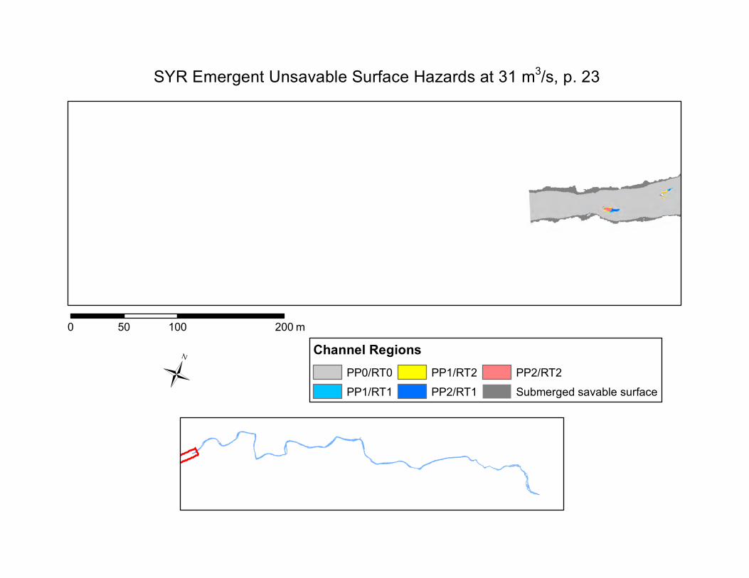
Channel RegionsPP0/RT0PP1/RT1
PP1/RT2PP2/RT1
PP2/RT2Submerged savable surface
0 100 20050 m
Ü
SYR Emergent Unsavable Surface Hazards at 31 m3/s, p. 23
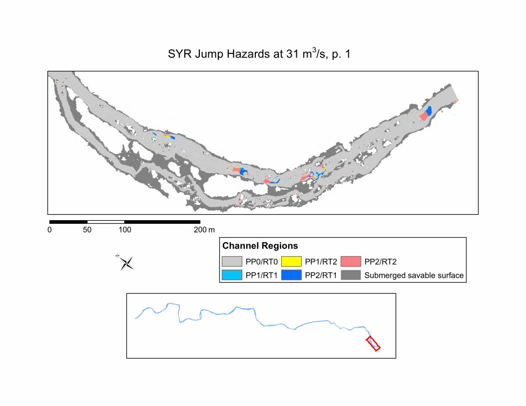
Channel RegionsPP0/RT0PP1/RT1
PP1/RT2PP2/RT1
PP2/RT2Submerged savable surface
0 100 20050 m
Ü
SYR Jump Hazards at 31 m3/s, p. 1
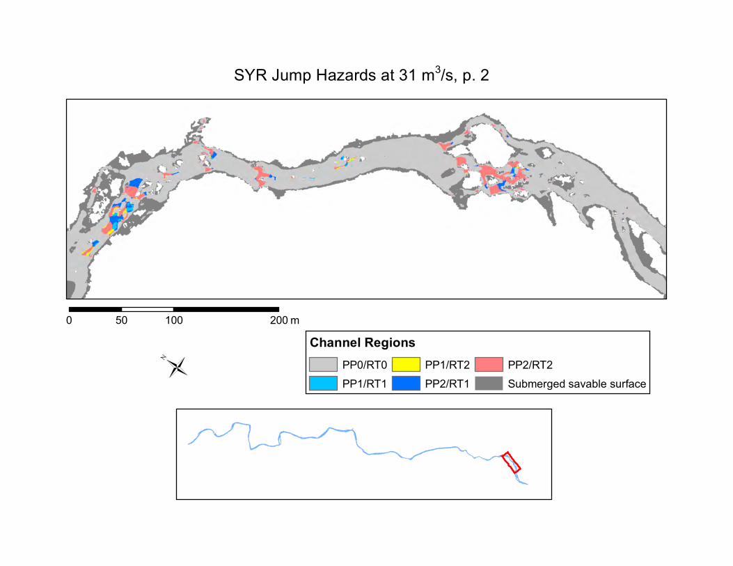
Channel RegionsPP0/RT0PP1/RT1
PP1/RT2PP2/RT1
PP2/RT2Submerged savable surface
0 100 20050 m
Ü
SYR Jump Hazards at 31 m3/s, p. 2

Channel RegionsPP0/RT0PP1/RT1
PP1/RT2PP2/RT1
PP2/RT2Submerged savable surface
0 100 20050 m
Ü
SYR Jump Hazards at 31 m3/s, p. 3
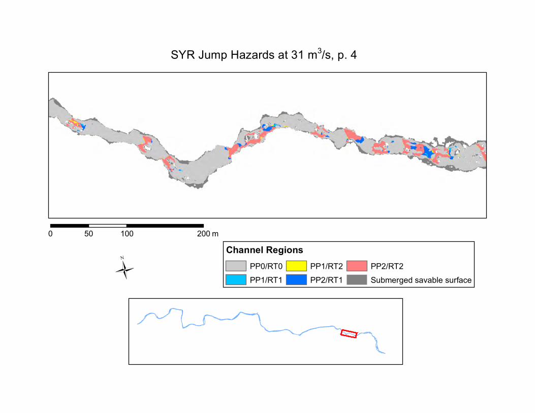
Channel RegionsPP0/RT0PP1/RT1
PP1/RT2PP2/RT1
PP2/RT2Submerged savable surface
0 100 20050 m
Ü
SYR Jump Hazards at 31 m3/s, p. 4
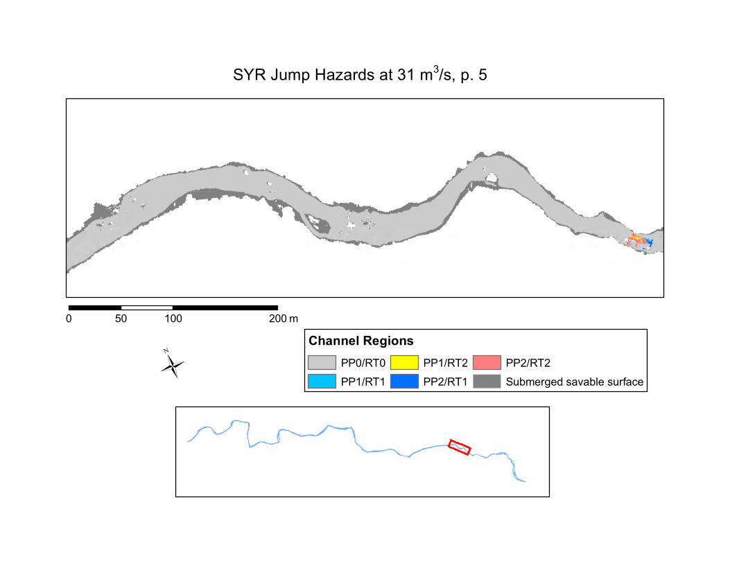
Channel RegionsPP0/RT0PP1/RT1
PP1/RT2PP2/RT1
PP2/RT2Submerged savable surface
0 100 20050 m
Ü
SYR Jump Hazards at 31 m3/s, p. 5

Channel RegionsPP0/RT0PP1/RT1
PP1/RT2PP2/RT1
PP2/RT2Submerged savable surface
0 100 20050 m
Ü
SYR Jump Hazards at 31 m3/s, p. 6
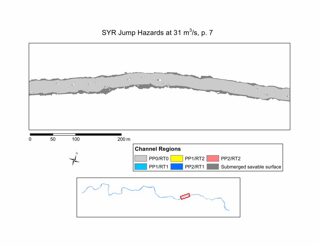
Channel RegionsPP0/RT0PP1/RT1
PP1/RT2PP2/RT1
PP2/RT2Submerged savable surface
0 100 20050 m
Ü
SYR Jump Hazards at 31 m3/s, p. 7
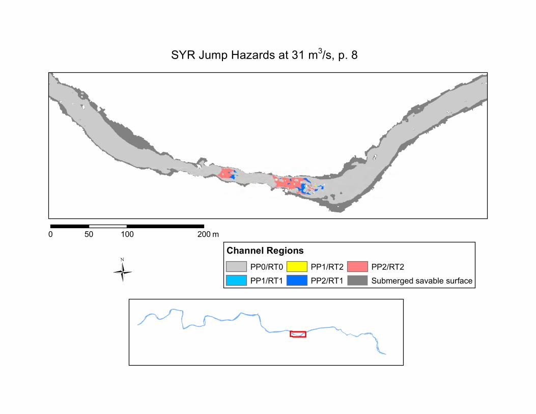
Channel RegionsPP0/RT0PP1/RT1
PP1/RT2PP2/RT1
PP2/RT2Submerged savable surface
0 100 20050 m
Ü
SYR Jump Hazards at 31 m3/s, p. 8
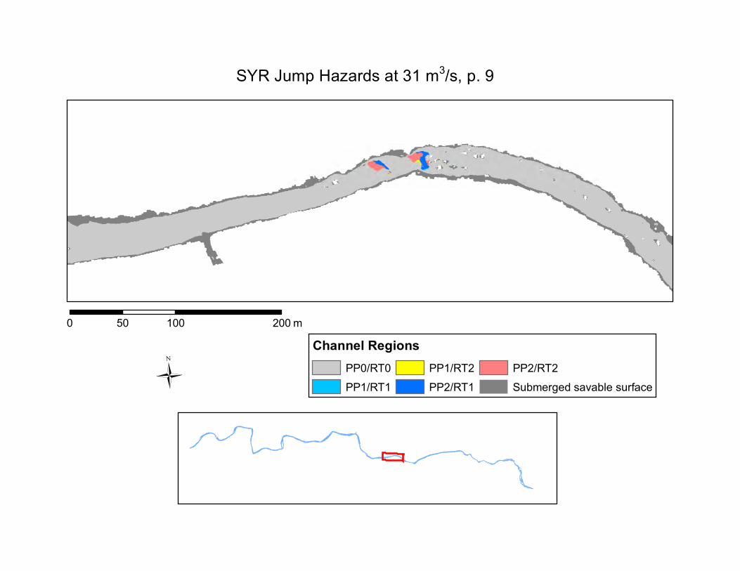
Channel RegionsPP0/RT0PP1/RT1
PP1/RT2PP2/RT1
PP2/RT2Submerged savable surface
0 100 20050 m
Ü
SYR Jump Hazards at 31 m3/s, p. 9
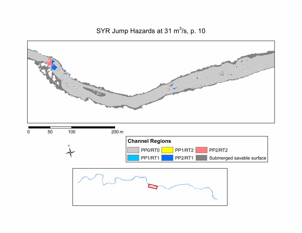
Channel RegionsPP0/RT0PP1/RT1
PP1/RT2PP2/RT1
PP2/RT2Submerged savable surface
0 100 20050 m
Ü
SYR Jump Hazards at 31 m3/s, p. 10
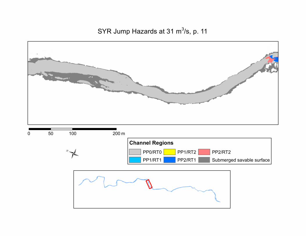
Channel RegionsPP0/RT0PP1/RT1
PP1/RT2PP2/RT1
PP2/RT2Submerged savable surface
0 100 20050 m
Ü
SYR Jump Hazards at 31 m3/s, p. 11

Channel RegionsPP0/RT0PP1/RT1
PP1/RT2PP2/RT1
PP2/RT2Submerged savable surface
0 100 20050 m
Ü
SYR Jump Hazards at 31 m3/s, p. 12

Channel RegionsPP0/RT0PP1/RT1
PP1/RT2PP2/RT1
PP2/RT2Submerged savable surface
0 100 20050 m
Ü
SYR Jump Hazards at 31 m3/s, p. 13

Channel RegionsPP0/RT0PP1/RT1
PP1/RT2PP2/RT1
PP2/RT2Submerged savable surface
0 100 20050 m
Ü
SYR Jump Hazards at 31 m3/s, p. 14

Channel RegionsPP0/RT0PP1/RT1
PP1/RT2PP2/RT1
PP2/RT2Submerged savable surface
0 100 20050 m
Ü
SYR Jump Hazards at 31 m3/s, p. 15

Channel RegionsPP0/RT0PP1/RT1
PP1/RT2PP2/RT1
PP2/RT2Submerged savable surface
0 100 20050 m
Ü
SYR Jump Hazards at 31 m3/s, p. 16

Channel RegionsPP0/RT0PP1/RT1
PP1/RT2PP2/RT1
PP2/RT2Submerged savable surface
0 100 20050 m
Ü
SYR Jump Hazards at 31 m3/s, p. 17
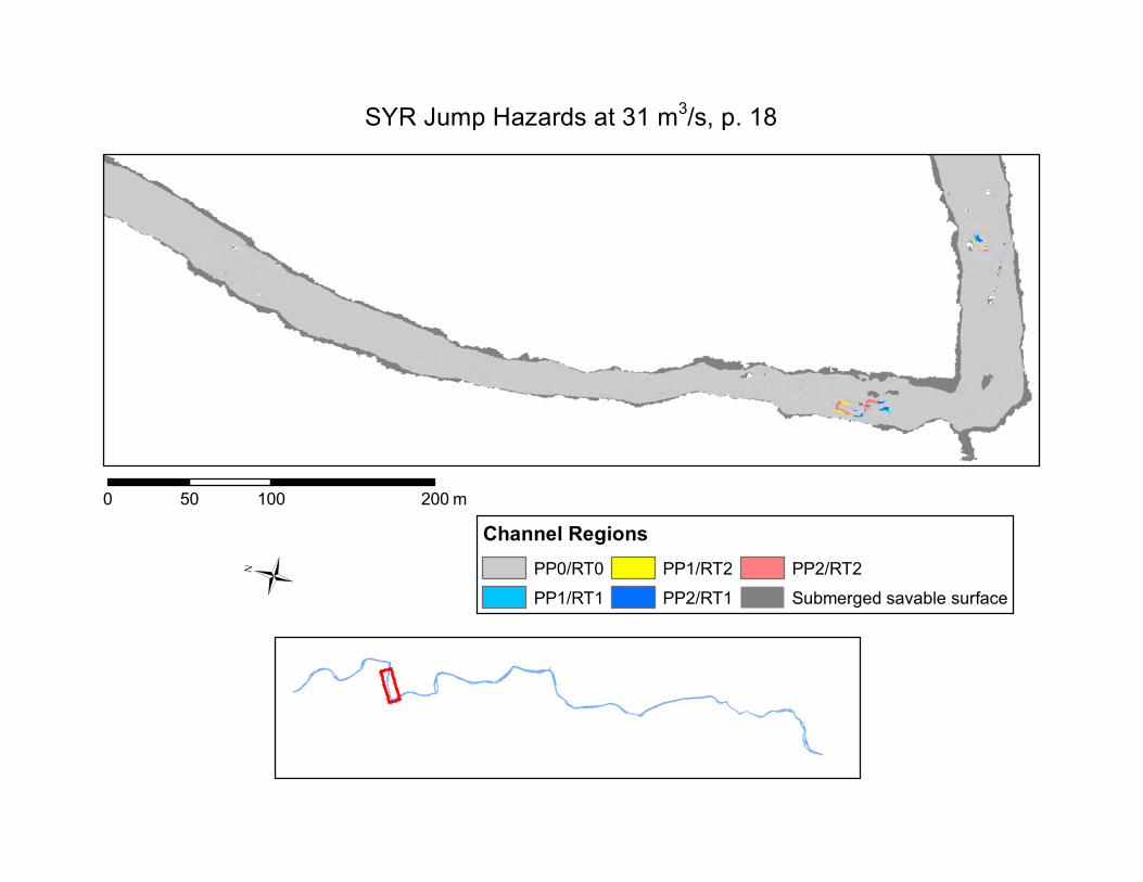
Channel RegionsPP0/RT0PP1/RT1
PP1/RT2PP2/RT1
PP2/RT2Submerged savable surface
0 100 20050 m
Ü
SYR Jump Hazards at 31 m3/s, p. 18
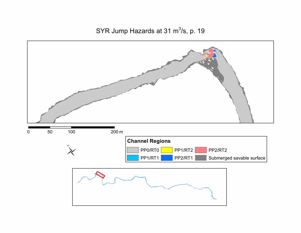
Channel RegionsPP0/RT0PP1/RT1
PP1/RT2PP2/RT1
PP2/RT2Submerged savable surface
0 100 20050 m
Ü
SYR Jump Hazards at 31 m3/s, p. 19
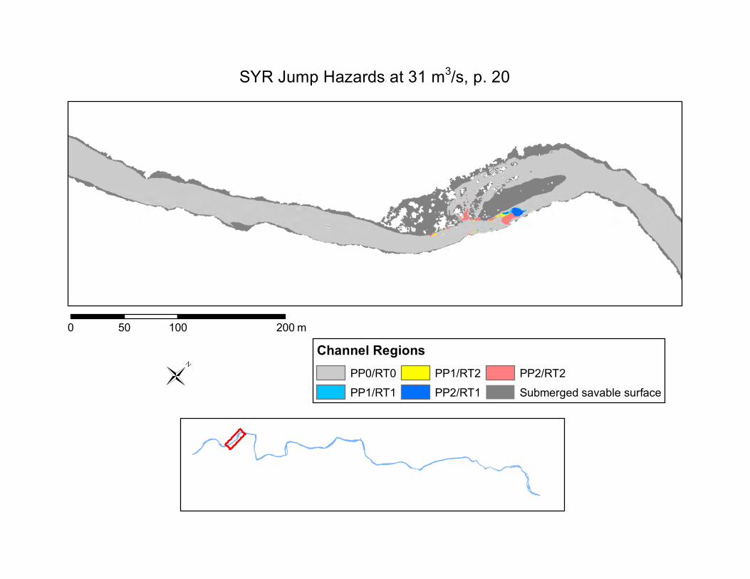
Channel RegionsPP0/RT0PP1/RT1
PP1/RT2PP2/RT1
PP2/RT2Submerged savable surface
0 100 20050 m
Ü
SYR Jump Hazards at 31 m3/s, p. 20
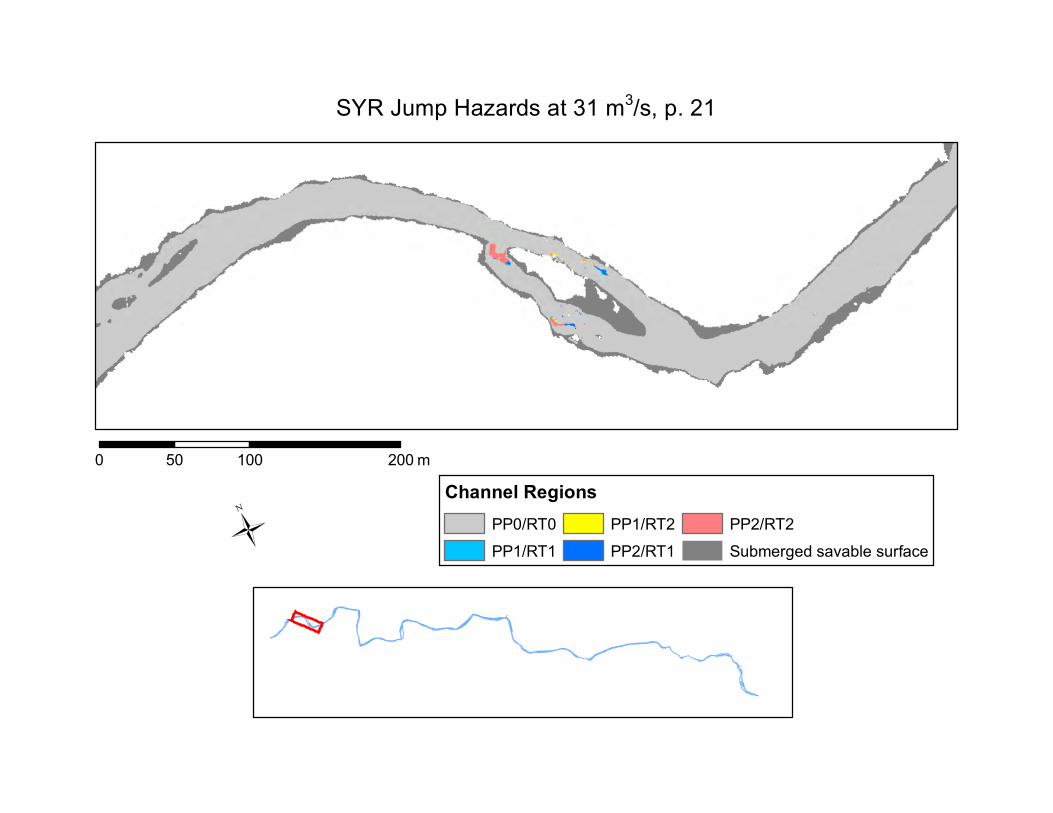
Channel RegionsPP0/RT0PP1/RT1
PP1/RT2PP2/RT1
PP2/RT2Submerged savable surface
0 100 20050 m
Ü
SYR Jump Hazards at 31 m3/s, p. 21
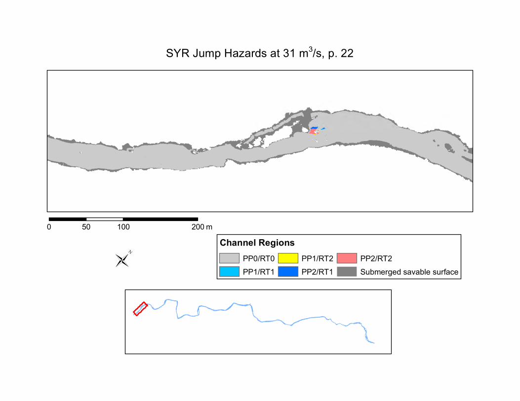
Channel RegionsPP0/RT0PP1/RT1
PP1/RT2PP2/RT1
PP2/RT2Submerged savable surface
0 100 20050 m
Ü
SYR Jump Hazards at 31 m3/s, p. 22
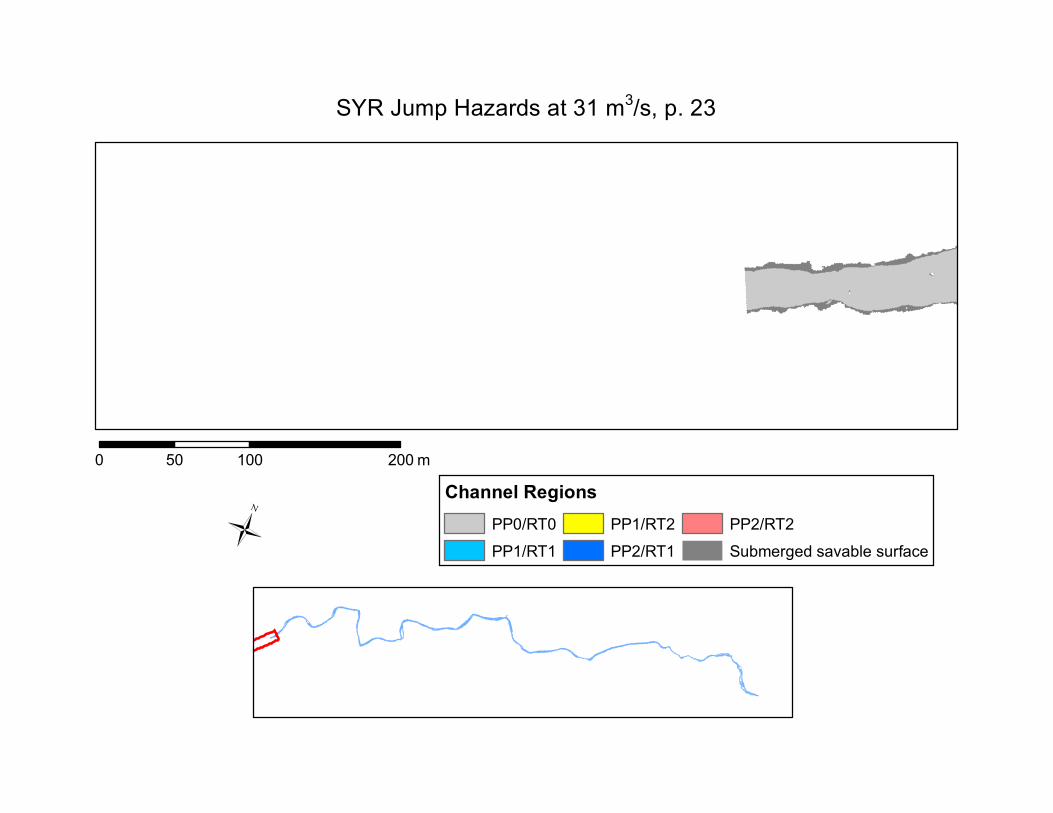
Channel RegionsPP0/RT0PP1/RT1
PP1/RT2PP2/RT1
PP2/RT2Submerged savable surface
0 100 20050 m
Ü
SYR Jump Hazards at 31 m3/s, p. 23

Channel RegionsPP0/RT0PP1/RT1
PP1/RT2PP2/RT1
PP2/RT2Submerged unsavable surface (PP3/RT3)Submerged savable surface
0 100 20050 m
Ü
SYR Submerged Unsavable Surface Hazards for Upright Body at 31 m3/s, p. 1
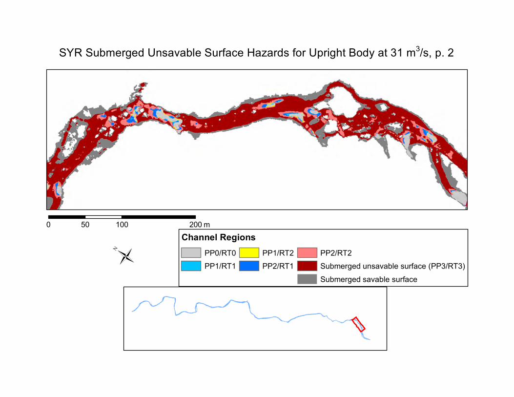
Channel RegionsPP0/RT0PP1/RT1
PP1/RT2PP2/RT1
PP2/RT2Submerged unsavable surface (PP3/RT3)Submerged savable surface
0 100 20050 m
Ü
SYR Submerged Unsavable Surface Hazards for Upright Body at 31 m3/s, p. 2

Channel RegionsPP0/RT0PP1/RT1
PP1/RT2PP2/RT1
PP2/RT2Submerged unsavable surface (PP3/RT3)Submerged savable surface
0 100 20050 m
Ü
SYR Submerged Unsavable Surface Hazards for Upright Body at 31 m3/s, p. 3
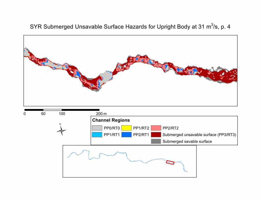
Channel RegionsPP0/RT0PP1/RT1
PP1/RT2PP2/RT1
PP2/RT2Submerged unsavable surface (PP3/RT3)Submerged savable surface
0 100 20050 m
Ü
SYR Submerged Unsavable Surface Hazards for Upright Body at 31 m3/s, p. 4
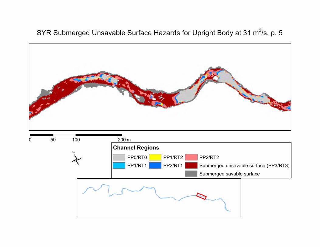
Channel RegionsPP0/RT0PP1/RT1
PP1/RT2PP2/RT1
PP2/RT2Submerged unsavable surface (PP3/RT3)Submerged savable surface
0 100 20050 m
Ü
SYR Submerged Unsavable Surface Hazards for Upright Body at 31 m3/s, p. 5
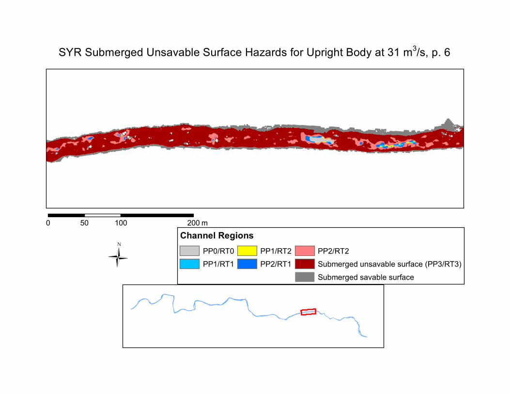
Channel RegionsPP0/RT0PP1/RT1
PP1/RT2PP2/RT1
PP2/RT2Submerged unsavable surface (PP3/RT3)Submerged savable surface
0 100 20050 m
Ü
SYR Submerged Unsavable Surface Hazards for Upright Body at 31 m3/s, p. 6

Channel RegionsPP0/RT0PP1/RT1
PP1/RT2PP2/RT1
PP2/RT2Submerged unsavable surface (PP3/RT3)Submerged savable surface
0 100 20050 m
Ü
SYR Submerged Unsavable Surface Hazards for Upright Body at 31 m3/s, p. 7
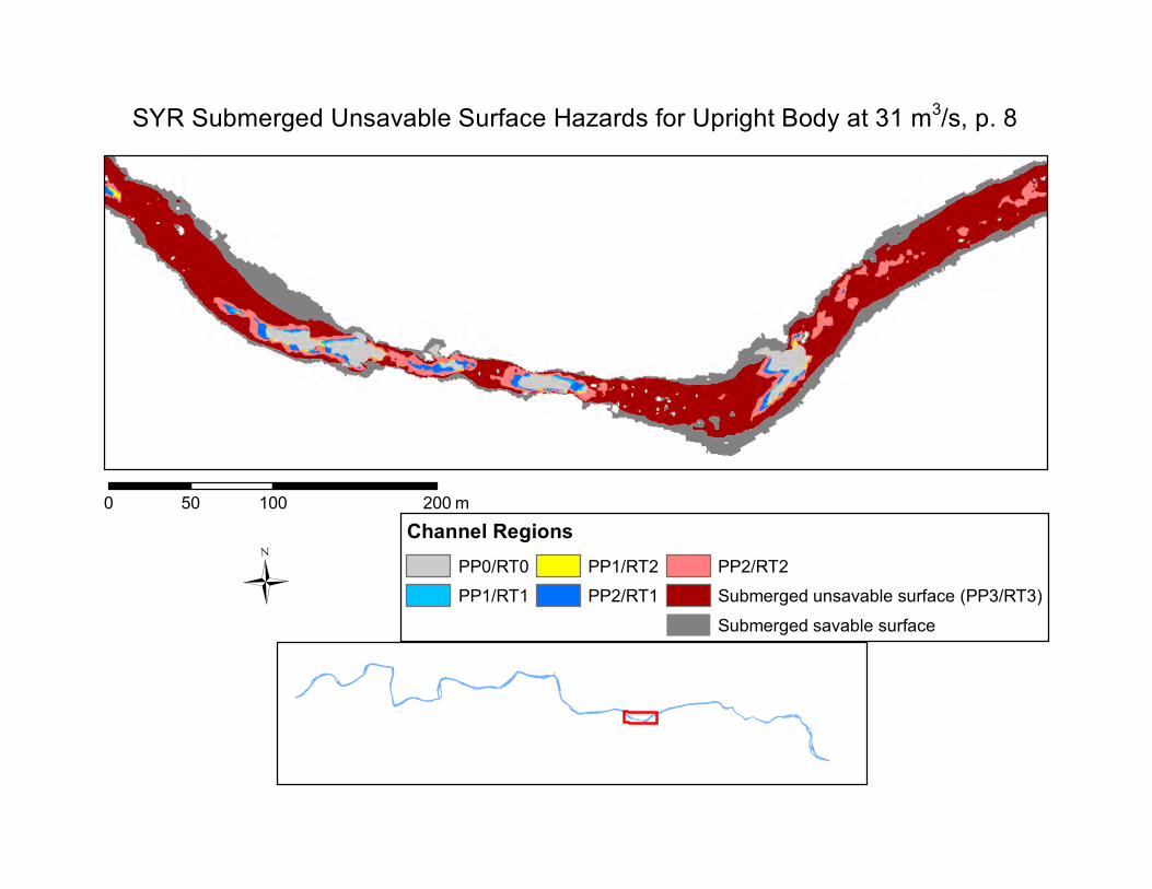
Channel RegionsPP0/RT0PP1/RT1
PP1/RT2PP2/RT1
PP2/RT2Submerged unsavable surface (PP3/RT3)Submerged savable surface
0 100 20050 m
Ü
SYR Submerged Unsavable Surface Hazards for Upright Body at 31 m3/s, p. 8
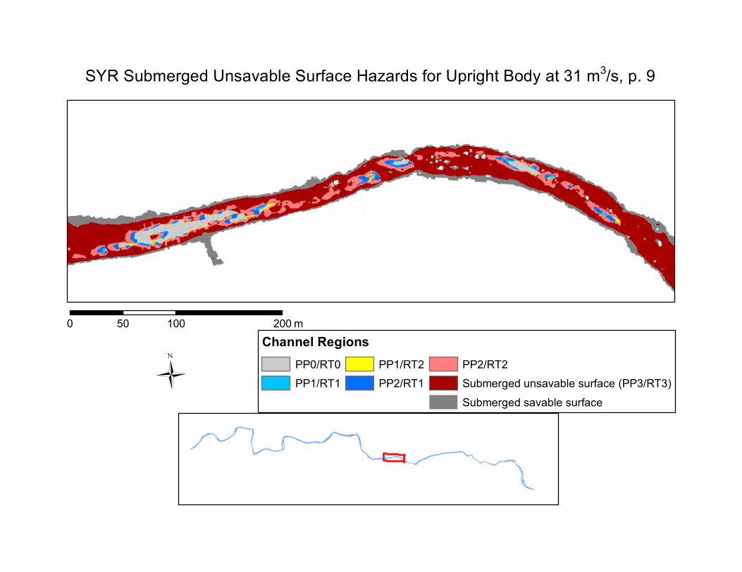
Channel RegionsPP0/RT0PP1/RT1
PP1/RT2PP2/RT1
PP2/RT2Submerged unsavable surface (PP3/RT3)Submerged savable surface
0 100 20050 m
Ü
SYR Submerged Unsavable Surface Hazards for Upright Body at 31 m3/s, p. 9
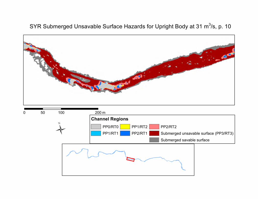
Channel RegionsPP0/RT0PP1/RT1
PP1/RT2PP2/RT1
PP2/RT2Submerged unsavable surface (PP3/RT3)Submerged savable surface
0 100 20050 m
Ü
SYR Submerged Unsavable Surface Hazards for Upright Body at 31 m3/s, p. 10
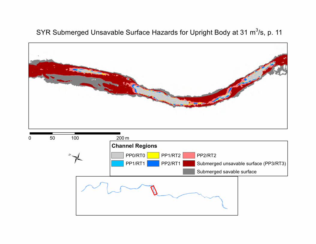
Channel RegionsPP0/RT0PP1/RT1
PP1/RT2PP2/RT1
PP2/RT2Submerged unsavable surface (PP3/RT3)Submerged savable surface
0 100 20050 m
Ü
SYR Submerged Unsavable Surface Hazards for Upright Body at 31 m3/s, p. 11

Channel RegionsPP0/RT0PP1/RT1
PP1/RT2PP2/RT1
PP2/RT2Submerged unsavable surface (PP3/RT3)Submerged savable surface
0 100 20050 m
Ü
SYR Submerged Unsavable Surface Hazards for Upright Body at 31 m3/s, p. 12

Channel RegionsPP0/RT0PP1/RT1
PP1/RT2PP2/RT1
PP2/RT2Submerged unsavable surface (PP3/RT3)Submerged savable surface
0 100 20050 m
Ü
SYR Submerged Unsavable Surface Hazards for Upright Body at 31 m3/s, p. 13

Channel RegionsPP0/RT0PP1/RT1
PP1/RT2PP2/RT1
PP2/RT2Submerged unsavable surface (PP3/RT3)Submerged savable surface
0 100 20050 m
Ü
SYR Submerged Unsavable Surface Hazards for Upright Body at 31 m3/s, p. 14

Channel RegionsPP0/RT0PP1/RT1
PP1/RT2PP2/RT1
PP2/RT2Submerged unsavable surface (PP3/RT3)Submerged savable surface
0 100 20050 m
Ü
SYR Submerged Unsavable Surface Hazards for Upright Body at 31 m3/s, p. 15
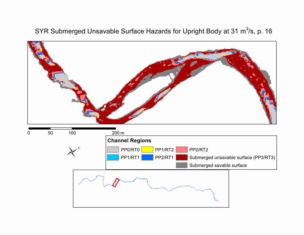
Channel RegionsPP0/RT0PP1/RT1
PP1/RT2PP2/RT1
PP2/RT2Submerged unsavable surface (PP3/RT3)Submerged savable surface
0 100 20050 m
Ü
SYR Submerged Unsavable Surface Hazards for Upright Body at 31 m3/s, p. 16

Channel RegionsPP0/RT0PP1/RT1
PP1/RT2PP2/RT1
PP2/RT2Submerged unsavable surface (PP3/RT3)Submerged savable surface
0 100 20050 m
Ü
SYR Submerged Unsavable Surface Hazards for Upright Body at 31 m3/s, p. 17
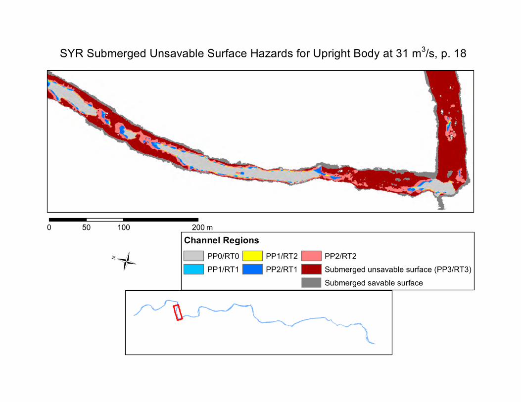
Channel RegionsPP0/RT0PP1/RT1
PP1/RT2PP2/RT1
PP2/RT2Submerged unsavable surface (PP3/RT3)Submerged savable surface
0 100 20050 m
Ü
SYR Submerged Unsavable Surface Hazards for Upright Body at 31 m3/s, p. 18
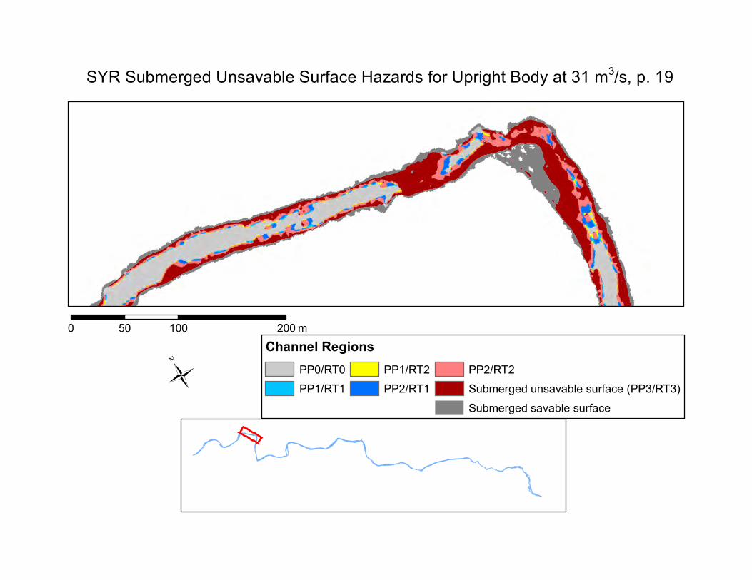
Channel RegionsPP0/RT0PP1/RT1
PP1/RT2PP2/RT1
PP2/RT2Submerged unsavable surface (PP3/RT3)Submerged savable surface
0 100 20050 m
Ü
SYR Submerged Unsavable Surface Hazards for Upright Body at 31 m3/s, p. 19
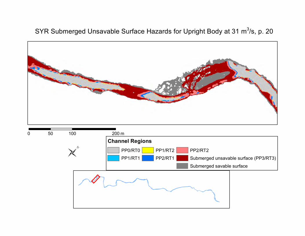
Channel RegionsPP0/RT0PP1/RT1
PP1/RT2PP2/RT1
PP2/RT2Submerged unsavable surface (PP3/RT3)Submerged savable surface
0 100 20050 m
Ü
SYR Submerged Unsavable Surface Hazards for Upright Body at 31 m3/s, p. 20

Channel RegionsPP0/RT0PP1/RT1
PP1/RT2PP2/RT1
PP2/RT2Submerged unsavable surface (PP3/RT3)Submerged savable surface
0 100 20050 m
Ü
SYR Submerged Unsavable Surface Hazards for Upright Body at 31 m3/s, p. 21
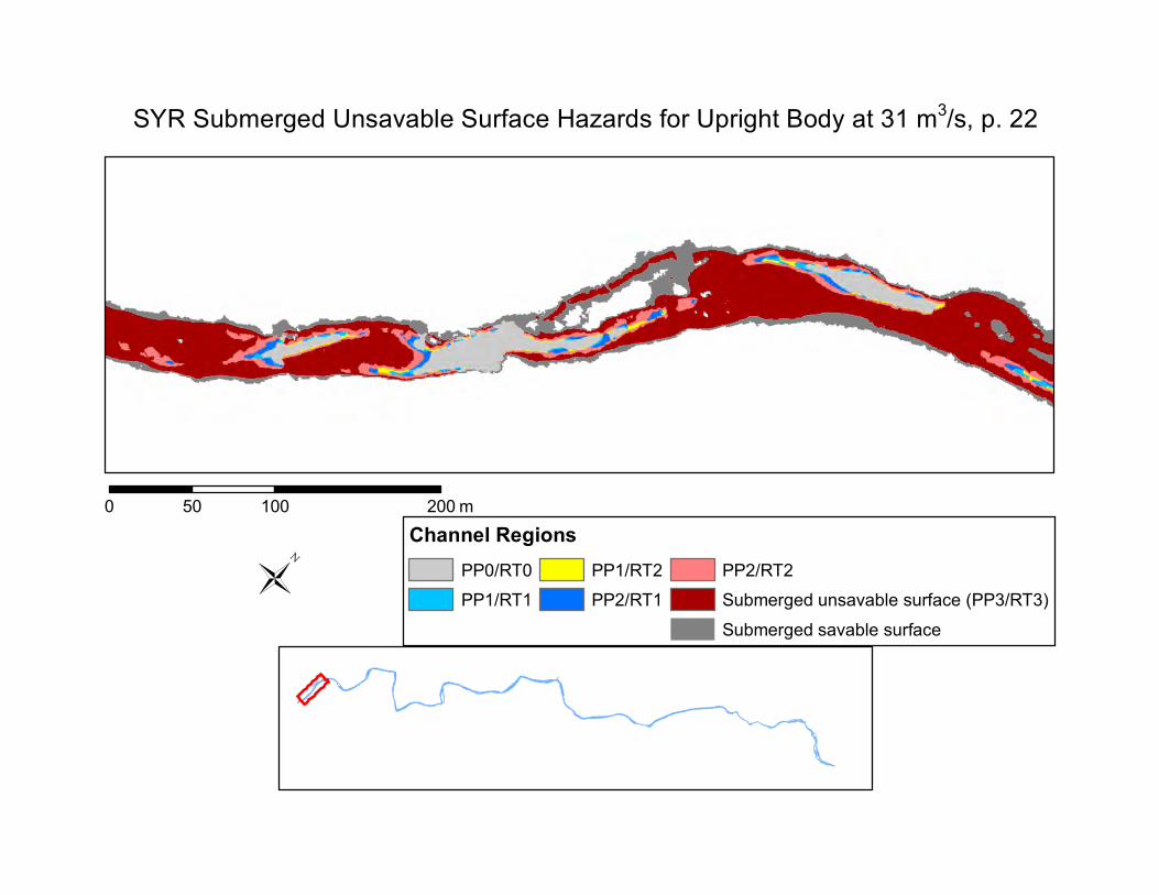
Channel RegionsPP0/RT0PP1/RT1
PP1/RT2PP2/RT1
PP2/RT2Submerged unsavable surface (PP3/RT3)Submerged savable surface
0 100 20050 m
Ü
SYR Submerged Unsavable Surface Hazards for Upright Body at 31 m3/s, p. 22
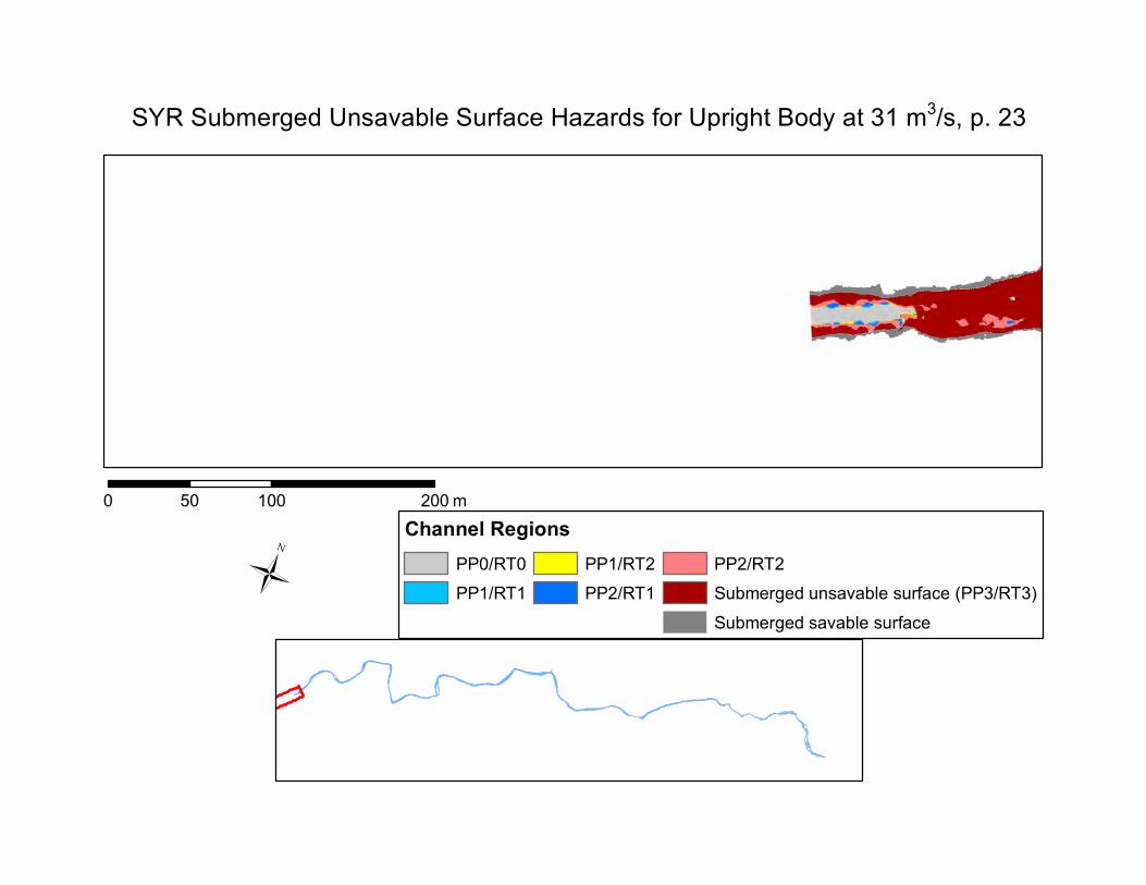
Channel RegionsPP0/RT0PP1/RT1
PP1/RT2PP2/RT1
PP2/RT2Submerged unsavable surface (PP3/RT3)Submerged savable surface
0 100 20050 m
Ü
SYR Submerged Unsavable Surface Hazards for Upright Body at 31 m3/s, p. 23
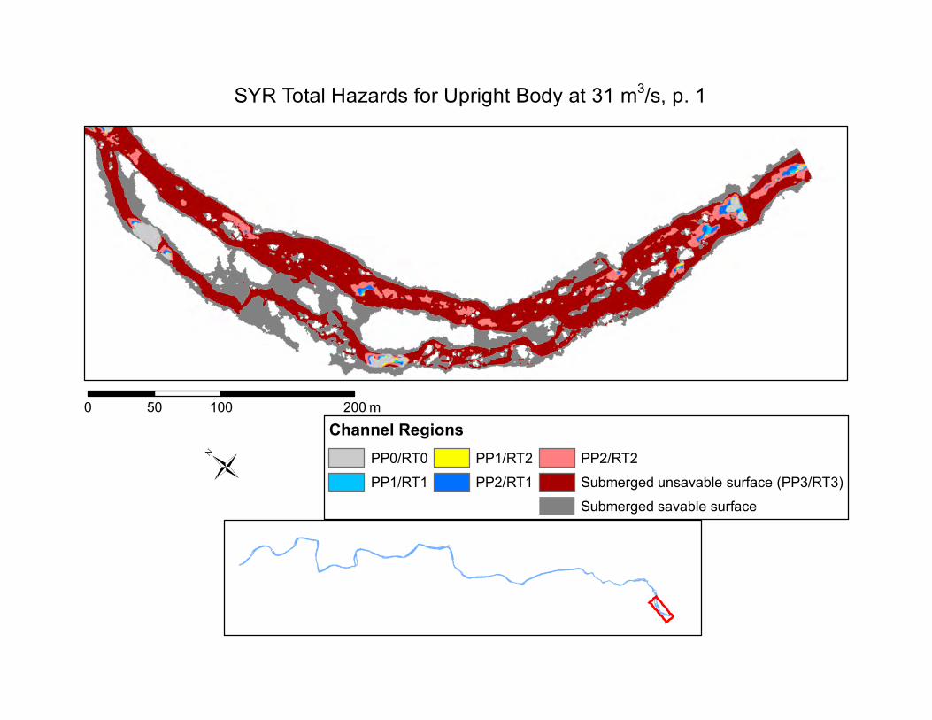
Channel RegionsPP0/RT0PP1/RT1
PP1/RT2PP2/RT1
PP2/RT2Submerged unsavable surface (PP3/RT3)Submerged savable surface
0 100 20050 m
Ü
SYR Total Hazards for Upright Body at 31 m3/s, p. 1

Channel RegionsPP0/RT0PP1/RT1
PP1/RT2PP2/RT1
PP2/RT2Submerged unsavable surface (PP3/RT3)Submerged savable surface
0 100 20050 m
Ü
SYR Total Hazards for Upright Body at 31 m3/s, p. 2
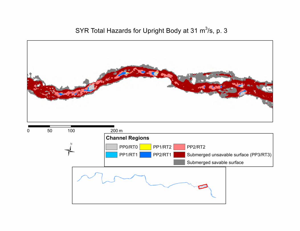
Channel RegionsPP0/RT0PP1/RT1
PP1/RT2PP2/RT1
PP2/RT2Submerged unsavable surface (PP3/RT3)Submerged savable surface
0 100 20050 m
Ü
SYR Total Hazards for Upright Body at 31 m3/s, p. 3
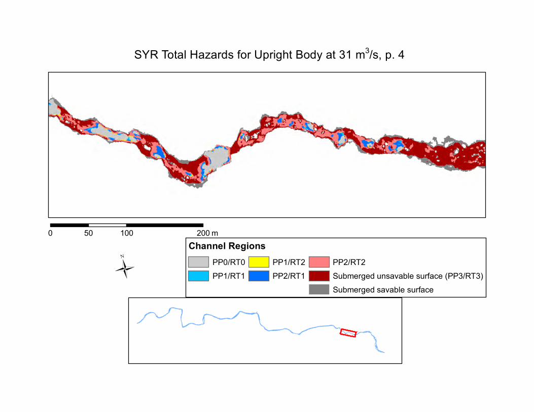
Channel RegionsPP0/RT0PP1/RT1
PP1/RT2PP2/RT1
PP2/RT2Submerged unsavable surface (PP3/RT3)Submerged savable surface
0 100 20050 m
Ü
SYR Total Hazards for Upright Body at 31 m3/s, p. 4

Channel RegionsPP0/RT0PP1/RT1
PP1/RT2PP2/RT1
PP2/RT2Submerged unsavable surface (PP3/RT3)Submerged savable surface
0 100 20050 m
Ü
SYR Total Hazards for Upright Body at 31 m3/s, p. 5

Channel RegionsPP0/RT0PP1/RT1
PP1/RT2PP2/RT1
PP2/RT2Submerged unsavable surface (PP3/RT3)Submerged savable surface
0 100 20050 m
Ü
SYR Total Hazards for Upright Body at 31 m3/s, p. 6

Channel RegionsPP0/RT0PP1/RT1
PP1/RT2PP2/RT1
PP2/RT2Submerged unsavable surface (PP3/RT3)Submerged savable surface
0 100 20050 m
Ü
SYR Total Hazards for Upright Body at 31 m3/s, p. 7
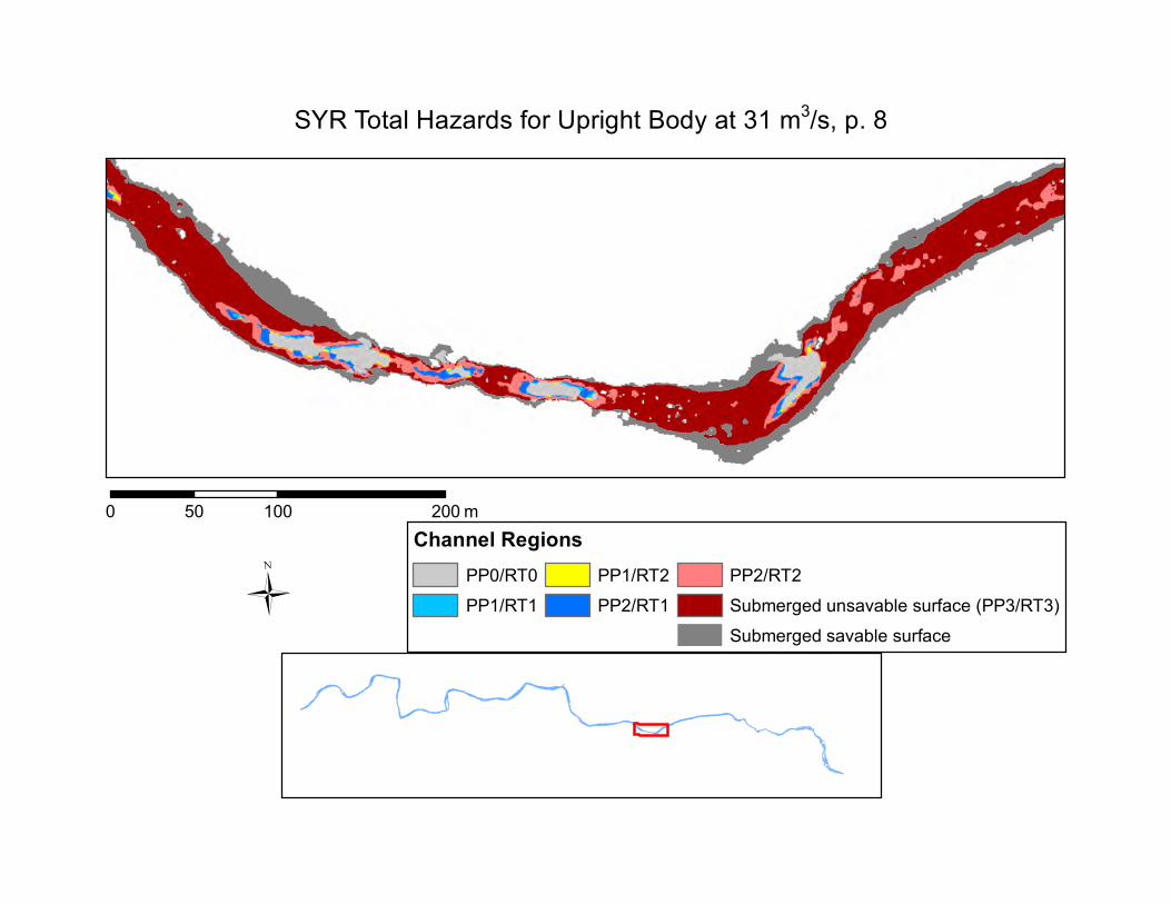
Channel RegionsPP0/RT0PP1/RT1
PP1/RT2PP2/RT1
PP2/RT2Submerged unsavable surface (PP3/RT3)Submerged savable surface
0 100 20050 m
Ü
SYR Total Hazards for Upright Body at 31 m3/s, p. 8
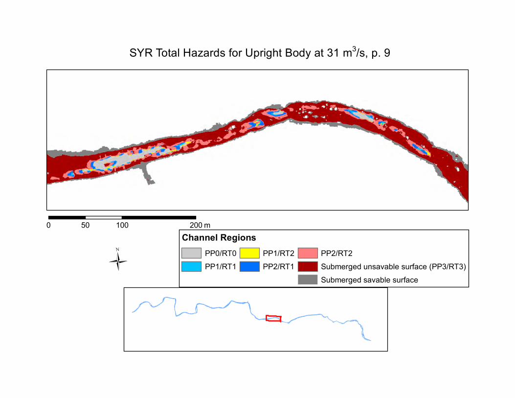
Channel RegionsPP0/RT0PP1/RT1
PP1/RT2PP2/RT1
PP2/RT2Submerged unsavable surface (PP3/RT3)Submerged savable surface
0 100 20050 m
Ü
SYR Total Hazards for Upright Body at 31 m3/s, p. 9
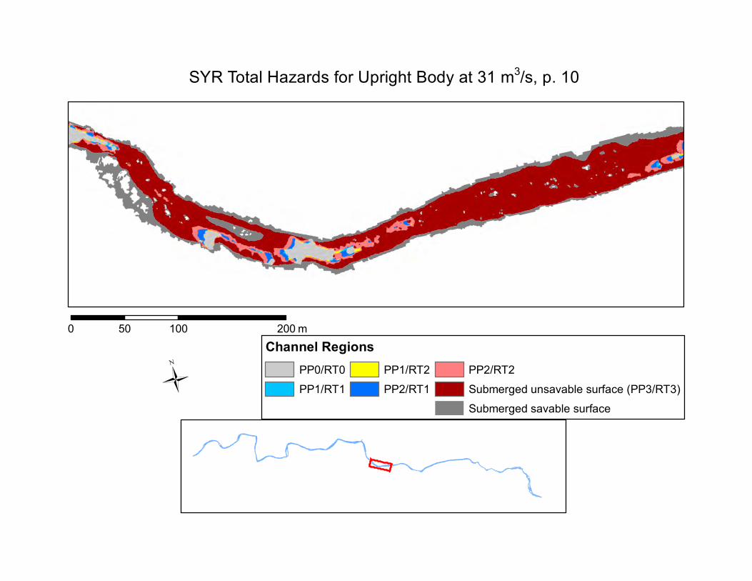
Channel RegionsPP0/RT0PP1/RT1
PP1/RT2PP2/RT1
PP2/RT2Submerged unsavable surface (PP3/RT3)Submerged savable surface
0 100 20050 m
Ü
SYR Total Hazards for Upright Body at 31 m3/s, p. 10
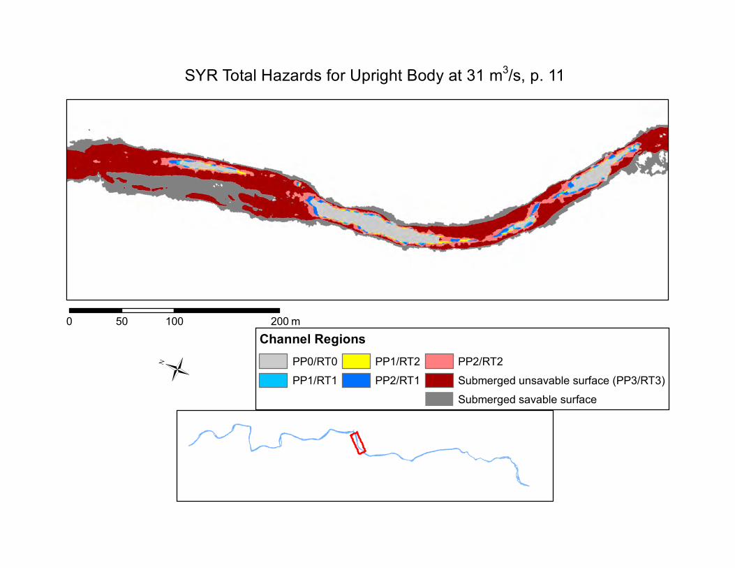
Channel RegionsPP0/RT0PP1/RT1
PP1/RT2PP2/RT1
PP2/RT2Submerged unsavable surface (PP3/RT3)Submerged savable surface
0 100 20050 m
Ü
SYR Total Hazards for Upright Body at 31 m3/s, p. 11
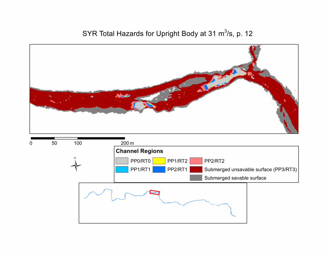
Channel RegionsPP0/RT0PP1/RT1
PP1/RT2PP2/RT1
PP2/RT2Submerged unsavable surface (PP3/RT3)Submerged savable surface
0 100 20050 m
Ü
SYR Total Hazards for Upright Body at 31 m3/s, p. 12
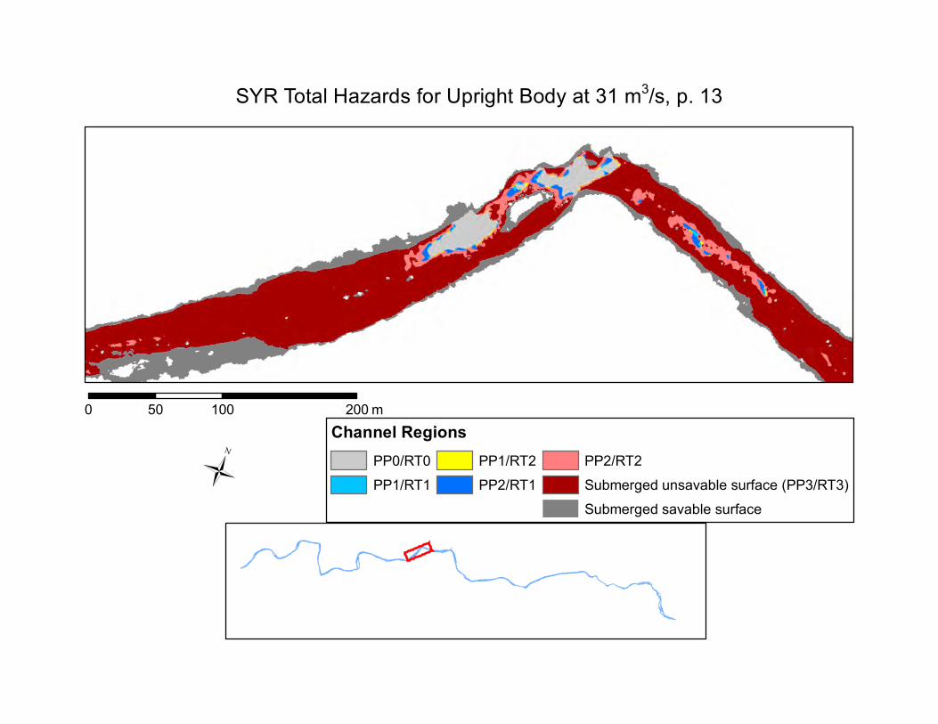
Channel RegionsPP0/RT0PP1/RT1
PP1/RT2PP2/RT1
PP2/RT2Submerged unsavable surface (PP3/RT3)Submerged savable surface
0 100 20050 m
Ü
SYR Total Hazards for Upright Body at 31 m3/s, p. 13
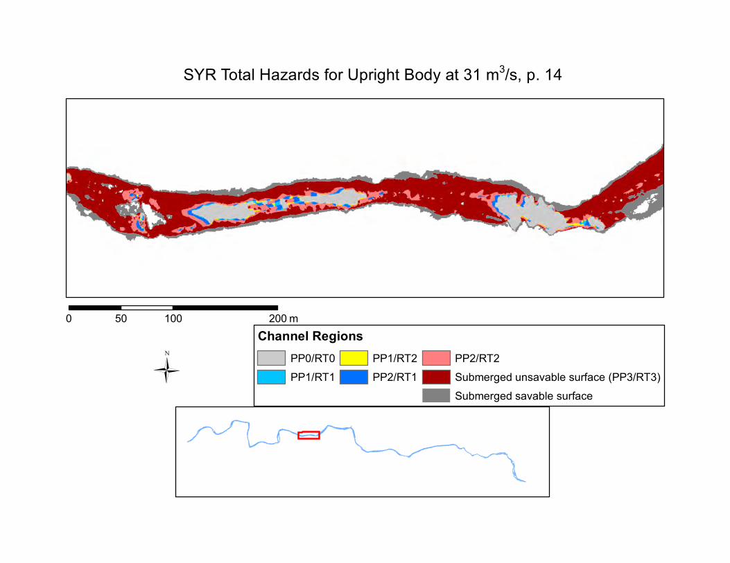
Channel RegionsPP0/RT0PP1/RT1
PP1/RT2PP2/RT1
PP2/RT2Submerged unsavable surface (PP3/RT3)Submerged savable surface
0 100 20050 m
Ü
SYR Total Hazards for Upright Body at 31 m3/s, p. 14
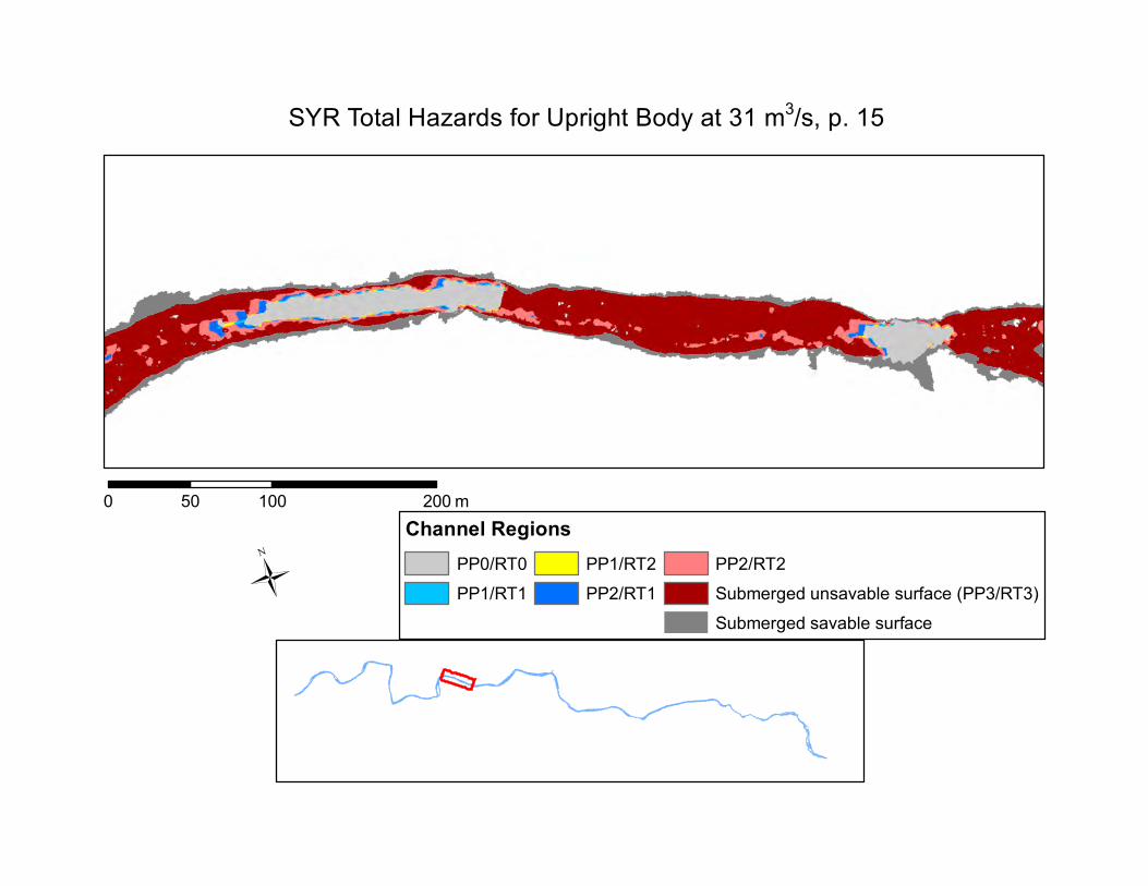
Channel RegionsPP0/RT0PP1/RT1
PP1/RT2PP2/RT1
PP2/RT2Submerged unsavable surface (PP3/RT3)Submerged savable surface
0 100 20050 m
Ü
SYR Total Hazards for Upright Body at 31 m3/s, p. 15

Channel RegionsPP0/RT0PP1/RT1
PP1/RT2PP2/RT1
PP2/RT2Submerged unsavable surface (PP3/RT3)Submerged savable surface
0 100 20050 m
Ü
SYR Total Hazards for Upright Body at 31 m3/s, p. 16
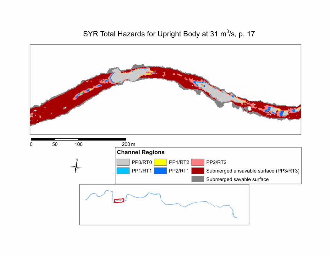
Channel RegionsPP0/RT0PP1/RT1
PP1/RT2PP2/RT1
PP2/RT2Submerged unsavable surface (PP3/RT3)Submerged savable surface
0 100 20050 m
Ü
SYR Total Hazards for Upright Body at 31 m3/s, p. 17

Channel RegionsPP0/RT0PP1/RT1
PP1/RT2PP2/RT1
PP2/RT2Submerged unsavable surface (PP3/RT3)Submerged savable surface
0 100 20050 m
Ü
SYR Total Hazards for Upright Body at 31 m3/s, p. 18

Channel RegionsPP0/RT0PP1/RT1
PP1/RT2PP2/RT1
PP2/RT2Submerged unsavable surface (PP3/RT3)Submerged savable surface
0 100 20050 m
Ü
SYR Total Hazards for Upright Body at 31 m3/s, p. 19

Channel RegionsPP0/RT0PP1/RT1
PP1/RT2PP2/RT1
PP2/RT2Submerged unsavable surface (PP3/RT3)Submerged savable surface
0 100 20050 m
Ü
SYR Total Hazards for Upright Body at 31 m3/s, p. 20
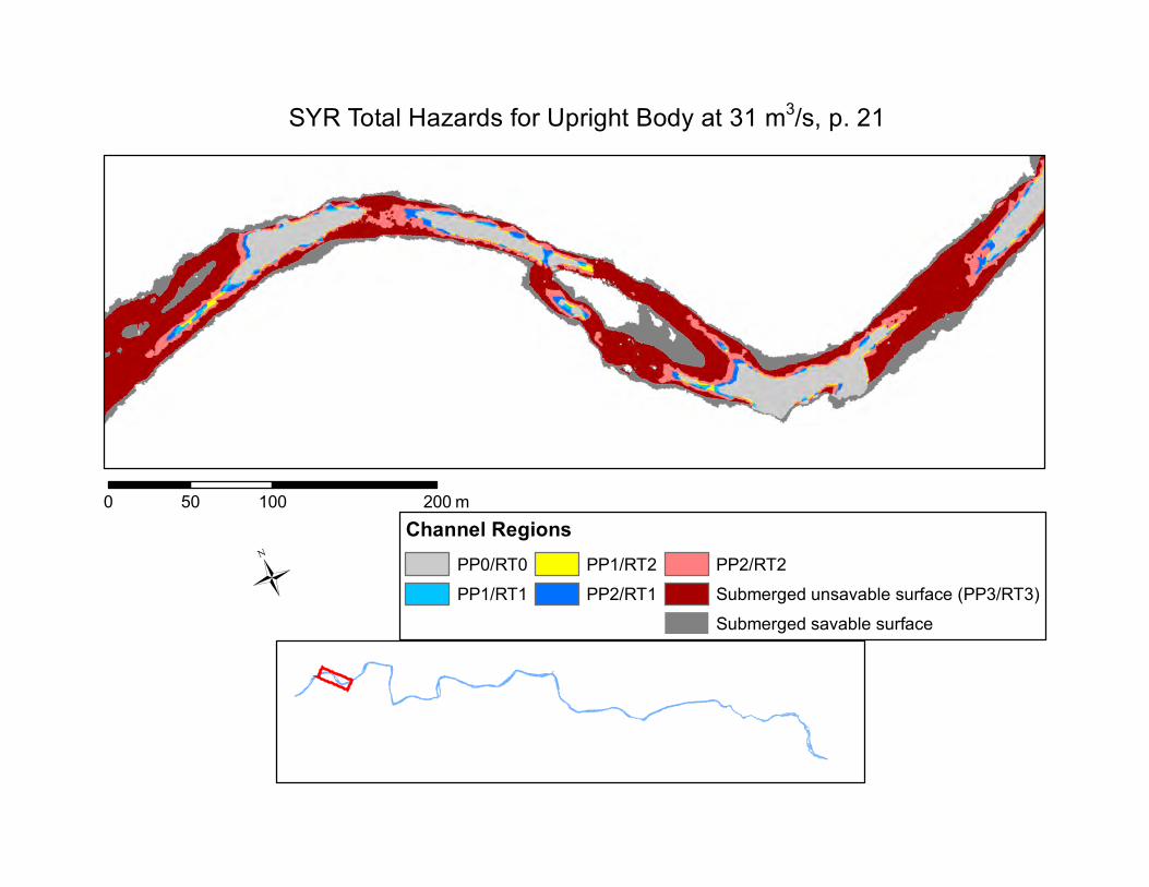
Channel RegionsPP0/RT0PP1/RT1
PP1/RT2PP2/RT1
PP2/RT2Submerged unsavable surface (PP3/RT3)Submerged savable surface
0 100 20050 m
Ü
SYR Total Hazards for Upright Body at 31 m3/s, p. 21

Channel RegionsPP0/RT0PP1/RT1
PP1/RT2PP2/RT1
PP2/RT2Submerged unsavable surface (PP3/RT3)Submerged savable surface
0 100 20050 m
Ü
SYR Total Hazards for Upright Body at 31 m3/s, p. 22
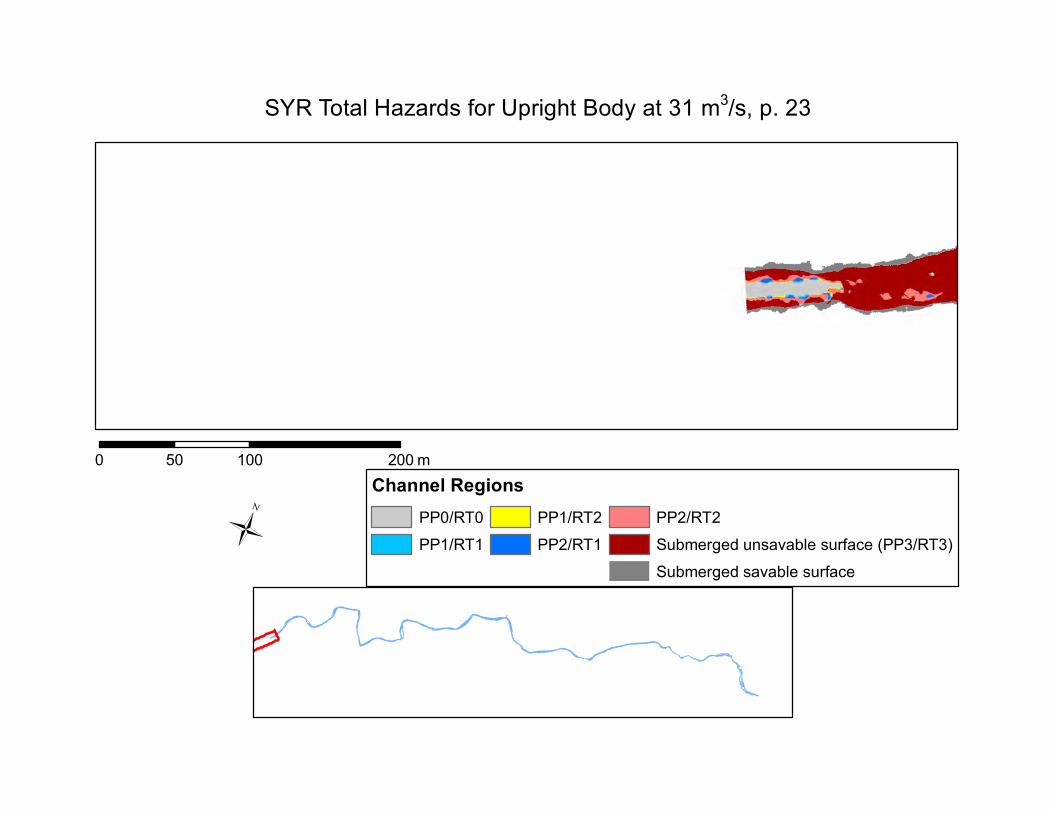
Channel RegionsPP0/RT0PP1/RT1
PP1/RT2PP2/RT1
PP2/RT2Submerged unsavable surface (PP3/RT3)Submerged savable surface
0 100 20050 m
Ü
SYR Total Hazards for Upright Body at 31 m3/s, p. 23