Copyright c© 2009 by Karl Sigman

1 IEOR 6711: Notes on the Poisson Process

We present here the essentials of the Poisson point process with its many interestingproperties. As preliminaries, we first define what a point process is, define the renewalpoint process and state and prove the Elementary Renewal Theorem.

1.1 Point Processes

Definition 1.1 A simple point process ψ = {tn : n ≥ 1} is a sequence of strictly increas-ing points

0 < t1 < t2 < · · · , (1)

with tn−→∞ as n−→∞. With N(0)def= 0 we let N(t) denote the number of points that

fall in the interval (0, t]; N(t) = max{n : tn ≤ t}. {N(t) : t ≥ 0} is called the countingprocess for ψ. If the tn are random variables then ψ is called a random point process.

We sometimes allow a point t0 at the origin and define t0def= 0. Xn = tn − tn−1, n ≥ 1,

is called the nth interarrival time.

We view t as time and view tn as the nth arrival time (although there are other kinds ofapplications in which the points tn denote locations in space as opposed to time). Theword simple refers to the fact that we are not allowing more than one arrival to ocurr atthe same time (as is stated precisely in (1)). In many applications there is a “system” towhich customers are arriving over time (classroom, bank, hospital, supermarket, airport,etc.), and {tn} denotes the arrival times of these customers to the system. But {tn} couldalso represent the times at which phone calls are received by a given phone, the timesat which jobs are sent to a printer in a computer network, the times at which a claim ismade against an insurance company, the times at which one receives or sends email, thetimes at which one sells or buys stock, the times at which a given web site receives hits,or the times at which subways arrive to a station. Note that

tn = X1 + · · ·+Xn, n ≥ 1,

the nth arrival time is the sum of the first n interarrival times.Also note that the event {N(t) = 0} can be equivalently represented by the event

{t1 > t}, and more generally

{N(t) = n} = {tn ≤ t, tn+1 > t}, n ≥ 1.

In particular, for a random point process, P (N(t) = 0) = P (t1 > t).

1

1.2 Renewal process

A random point process ψ = {tn} for which the interarrival times {Xn} form an i.i.d.sequence is called a renewal process. tn is then called the nth renewal epoch and F (x) =P (X ≤ x), x ≥ 0, denotes the common interarrival time distribution. To avoid trivialitieswe always assume that F (0) < 1, hence ensuring that wp1, tn → ∞. The rate of the

renewal process is defined as λdef= 1/E(X) which is justified by

Theorem 1.1 (Elementary Renewal Theorem (ERT)) For a renewal process,

limt→∞

N(t)

t= λ w.p.1.

and

limt→∞

E(N(t))

t= λ.

Proof : Observing that tN(t) ≤ t < tN(t)+1 and that tN(t) = X1 + · · ·XN(t), yields afterdivision by N(t):

1

N(t)

N(t)∑j=1

Xj ≤t

N(t)≤ 1

N(t)

N(t)+1∑j=1

Xj.

By the Strong Law of Large Numbers (SLLN), both the left and the right pieces convergeto E(X) as t−→∞. Since t/N(t) is sandwiched between the two, it also converges toE(X), yielding the first result after taking reciprocals.

For the second result, we must show that the collection of rvs {N(t)/t : t ≥ 1} isuniformly integrable (UI)1, so as to justify the interchange of limit and expected value,

limt→∞

E(N(t))

t= E

(limt→∞

N(t)

t

).

We will show that P (N(t)/t > x) ≤ c/x2, x > 0 for some c > 0 hence proving UI. To thisend, choose a > 0 such that 0 < F (a) < 1 (if no such a exists then the renewal process isdeterministic and the result is trival). Define new interarrival times via truncation X̂n =aI{Xn > a}. Thus X̂n = 0 with probability F (a) and equals a with probability 1−F (a).Letting N̂(t) denote the counting process obtained by using these new interarrival times,it follows that N(t) ≤ N̂(t), t ≥ 0. Moreover, arrivals (which now occur in batches) cannow only occur at the deterministic lattice of times {na : n ≥ 0}. Letting p = 1− F (a),and letting Kn denote the number of arrivals that occur at time na, we conclude that{Kn} is iid with a geometric distribution with success probability p. Letting [x] denotethe smallest integer ≥ x, we have the inequality

N(t) ≤ N̂(t) ≤ S(t) =

[t/a]∑n=1

Kn, t ≥ 0.

1A collection of rvs {Xt : t ∈ T} is said to be uniformly integrable (UI), if supt∈T E(|Xt|I{|Xt| >x})→ 0, as x→∞.

2

Observing that E(S(t)) = [t/a]E(K) and V ar(S(t)) = [t/a]V ar(K), we obtainE(S(t)2) =V ar(S(t) + E(S(t))2 = [t/a]V ar(K) + [t/a]2E2(K) ≤ c1t + c2t

2, for constants c1 >0, c2 > 0. Finally, when t ≥ 1, Chebychev’s inequality implies that P (N(t)/t > x) ≤E(N2(t))/t2x2 ≤ E(S2(t))/t2x2 ≤ c/x2 where c = c1 + c2.

Remark 1.1 In the elementary renewal theorem, the case when λ = 0 (e.g., E(X) =∞)is allowed, in which case the renewal process is said to be null recurrent. In the case when0 < λ <∞ (e.g., 0 < E(X) <∞ ) the renewal process is said to be positive recurrent.

1.3 Poisson point process

There are several equivalent definitions for a Poisson process; we present the simplestone. Although this definition does not indicate why the word “Poisson” is used, that willbe made apparent soon. Recall that a renewal process is a point process ψ = {tn : n ≥ 0}in which the interarrival times Xn = tn − tn−1 are i.i.d. r.v.s. with common distributionF (x) = P (X ≤ x). The arrival rate is given by λ = {E(X)}−1 which is justified by theERT (Theorem 1.1).

In what follows it helps to imagine that the arrival times tn correspond to the consec-utive times that a subway arrives to your station, and that you are interested in catchingthe next subway.

Definition 1.2 A Poisson process at rate 0 < λ < ∞ is a renewal point process inwhich the interarrival time distribution is exponential with rate λ: interarrival times{Xn : n ≥ 1} are i.i.d. with common distribution F (x) = P (X ≤ x) = 1− e−λx, x ≥ 0;E(X) = 1/λ.

Since tn = X1 + · · · + Xn (the sum of n i.i.d. exponentially distributed r.v.s.), weconclude that the distribution of tn is the nth-fold convolution of the exponential distri-bution and thus is a gamma(n, λ) distribution (also called an Erlang(n, λ) distribution);its density is given by

fn(t) = λe−λt(λt)n−1

(n− 1)!, t ≥ 0, (2)

where f1(t) = f(t) = λe−λt is the exponential density, and E(tn) = E(X1 + · · ·+Xn) =nE(X) = n/λ.

For example, f2 is the convolution f1 ∗ f1:

f2(t) =

∫ t

0

f1(t− s)f1(s)ds

=

∫ t

0

λe−λ(t−s)dsλe−λsds

= λe−λt∫ t

0

λds

= λe−λtλt,

3

and in general fn+1 = fn ∗ f1 = f1 ∗ fn.

1.4 The Poisson distribution: A Poisson process has Poissonincrements

Later, in Section 1.6 we will prove the fundamental fact that: For each fixed t > 0, thedistribution of N(t) is Poisson with mean λt:

P (N(t) = k) = e−λt(λt)k

k!, k ≥ 0.

In particular, E(N(t)) = λt, V ar(N(t)) = λt, t ≥ 0. In fact, the number of arrivals inany arbitrary interval of length t, N(s+ t)−N(s) is also Poisson with mean λt:

P (N(s+ t)−N(s) = k) = e−λt(λt)k

k!, s > 0, k ≥ 0,

and E(N(s+ t)−N(s)) = λt, V ar(N(s+ t)−N(s)) = λt, t ≥ 0.N(s+t)−N(s) is called a length t increment of the counting process {N(t) : t ≥ 0}; the

above tells us that the Poisson counting process has increments that have a distributionthat is Poisson and only depends on the length of the increment. Any increment of lengtht is distributed as Poisson with mean λt.

1.5 Review of the exponential distribution

The exponential distribution has many nice properties; we review them next.A r.v. X has an exponential distribution at rate λ, denoted by X ∼ exp(λ), if X

is non-negative with c.d.f. F (x) = P (X ≤ x), tail F (x) = P (X > x) = 1 − F (x) anddensity f(x) = F ′(x) given by

F (x) = 1− e−λx, x ≥ 0,

F (x) = e−λx, x ≥ 0,

f(x) = λe−λx, x ≥ 0.

It is easily seen that

E(X) =1

λ

E(X2) =2

λ2

V ar(X) =1

λ2.

4

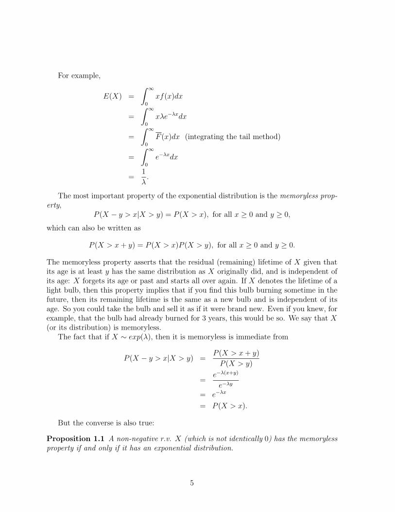
For example,

E(X) =

∫ ∞0

xf(x)dx

=

∫ ∞0

xλe−λxdx

=

∫ ∞0

F (x)dx (integrating the tail method)

=

∫ ∞0

e−λxdx

=1

λ.

The most important property of the exponential distribution is the memoryless prop-erty,

P (X − y > x|X > y) = P (X > x), for all x ≥ 0 and y ≥ 0,

which can also be written as

P (X > x+ y) = P (X > x)P (X > y), for all x ≥ 0 and y ≥ 0.

The memoryless property asserts that the residual (remaining) lifetime of X given thatits age is at least y has the same distribution as X originally did, and is independent ofits age: X forgets its age or past and starts all over again. If X denotes the lifetime of alight bulb, then this property implies that if you find this bulb burning sometime in thefuture, then its remaining lifetime is the same as a new bulb and is independent of itsage. So you could take the bulb and sell it as if it were brand new. Even if you knew, forexample, that the bulb had already burned for 3 years, this would be so. We say that X(or its distribution) is memoryless.

The fact that if X ∼ exp(λ), then it is memoryless is immediate from

P (X − y > x|X > y) =P (X > x+ y)

P (X > y)

=e−λ(x+y)

e−λy

= e−λx

= P (X > x).

But the converse is also true:

Proposition 1.1 A non-negative r.v. X (which is not identically 0) has the memorylessproperty if and only if it has an exponential distribution.

5

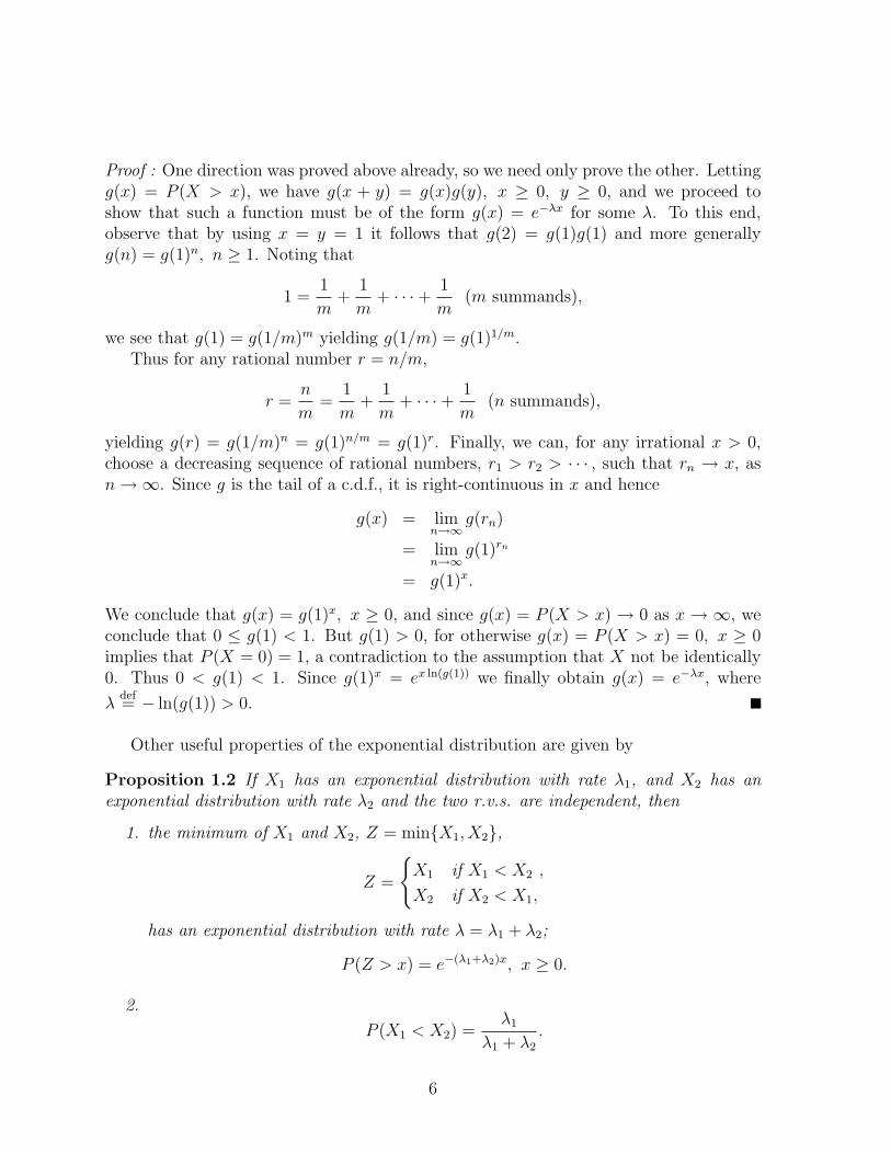
Proof : One direction was proved above already, so we need only prove the other. Lettingg(x) = P (X > x), we have g(x + y) = g(x)g(y), x ≥ 0, y ≥ 0, and we proceed toshow that such a function must be of the form g(x) = e−λx for some λ. To this end,observe that by using x = y = 1 it follows that g(2) = g(1)g(1) and more generallyg(n) = g(1)n, n ≥ 1. Noting that

1 =1

m+

1

m+ · · ·+ 1

m(m summands),

we see that g(1) = g(1/m)m yielding g(1/m) = g(1)1/m.Thus for any rational number r = n/m,

r =n

m=

1

m+

1

m+ · · ·+ 1

m(n summands),

yielding g(r) = g(1/m)n = g(1)n/m = g(1)r. Finally, we can, for any irrational x > 0,choose a decreasing sequence of rational numbers, r1 > r2 > · · · , such that rn → x, asn→∞. Since g is the tail of a c.d.f., it is right-continuous in x and hence

g(x) = limn→∞

g(rn)

= limn→∞

g(1)rn

= g(1)x.

We conclude that g(x) = g(1)x, x ≥ 0, and since g(x) = P (X > x) → 0 as x → ∞, weconclude that 0 ≤ g(1) < 1. But g(1) > 0, for otherwise g(x) = P (X > x) = 0, x ≥ 0implies that P (X = 0) = 1, a contradiction to the assumption that X not be identically0. Thus 0 < g(1) < 1. Since g(1)x = ex ln(g(1)) we finally obtain g(x) = e−λx, where

λdef= − ln(g(1)) > 0.

Other useful properties of the exponential distribution are given by

Proposition 1.2 If X1 has an exponential distribution with rate λ1, and X2 has anexponential distribution with rate λ2 and the two r.v.s. are independent, then

1. the minimum of X1 and X2, Z = min{X1, X2},

Z =

{X1 if X1 < X2 ,

X2 if X2 < X1,

has an exponential distribution with rate λ = λ1 + λ2;

P (Z > x) = e−(λ1+λ2)x, x ≥ 0.

2.

P (X1 < X2) =λ1

λ1 + λ2

.

6

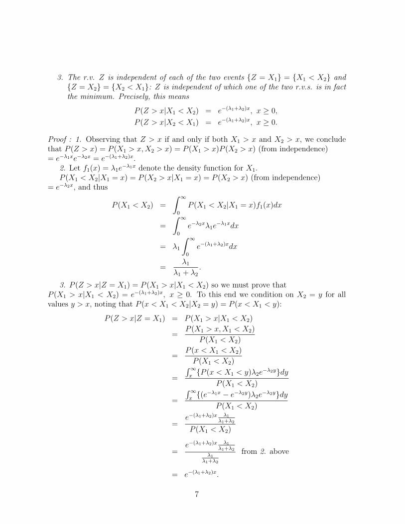
3. The r.v. Z is independent of each of the two events {Z = X1} = {X1 < X2} and{Z = X2} = {X2 < X1}: Z is independent of which one of the two r.v.s. is in factthe minimum. Precisely, this means

P (Z > x|X1 < X2) = e−(λ1+λ2)x, x ≥ 0,

P (Z > x|X2 < X1) = e−(λ1+λ2)x, x ≥ 0.

Proof : 1. Observing that Z > x if and only if both X1 > x and X2 > x, we concludethat P (Z > x) = P (X1 > x,X2 > x) = P (X1 > x)P (X2 > x) (from independence)= e−λ1xe−λ2x = e−(λ1+λ2)x.

2. Let f1(x) = λ1e−λ1x denote the density function for X1.

P (X1 < X2|X1 = x) = P (X2 > x|X1 = x) = P (X2 > x) (from independence)= e−λ2x, and thus

P (X1 < X2) =

∫ ∞0

P (X1 < X2|X1 = x)f1(x)dx

=

∫ ∞0

e−λ2xλ1e−λ1xdx

= λ1

∫ ∞0

e−(λ1+λ2)xdx

=λ1

λ1 + λ2

.

3. P (Z > x|Z = X1) = P (X1 > x|X1 < X2) so we must prove thatP (X1 > x|X1 < X2) = e−(λ1+λ2)x, x ≥ 0. To this end we condition on X2 = y for allvalues y > x, noting that P (x < X1 < X2|X2 = y) = P (x < X1 < y):

P (Z > x|Z = X1) = P (X1 > x|X1 < X2)

=P (X1 > x,X1 < X2)

P (X1 < X2)

=P (x < X1 < X2)

P (X1 < X2)

=

∫∞x{P (x < X1 < y)λ2e

−λ2y}dyP (X1 < X2)

=

∫∞x{(e−λ1x − e−λ2y)λ2e

−λ2y}dyP (X1 < X2)

=e−(λ1+λ2)x λ1

λ1+λ2

P (X1 < X2)

=e−(λ1+λ2)x λ1

λ1+λ2

λ1

λ1+λ2

from 2. above

= e−(λ1+λ2)x.

7

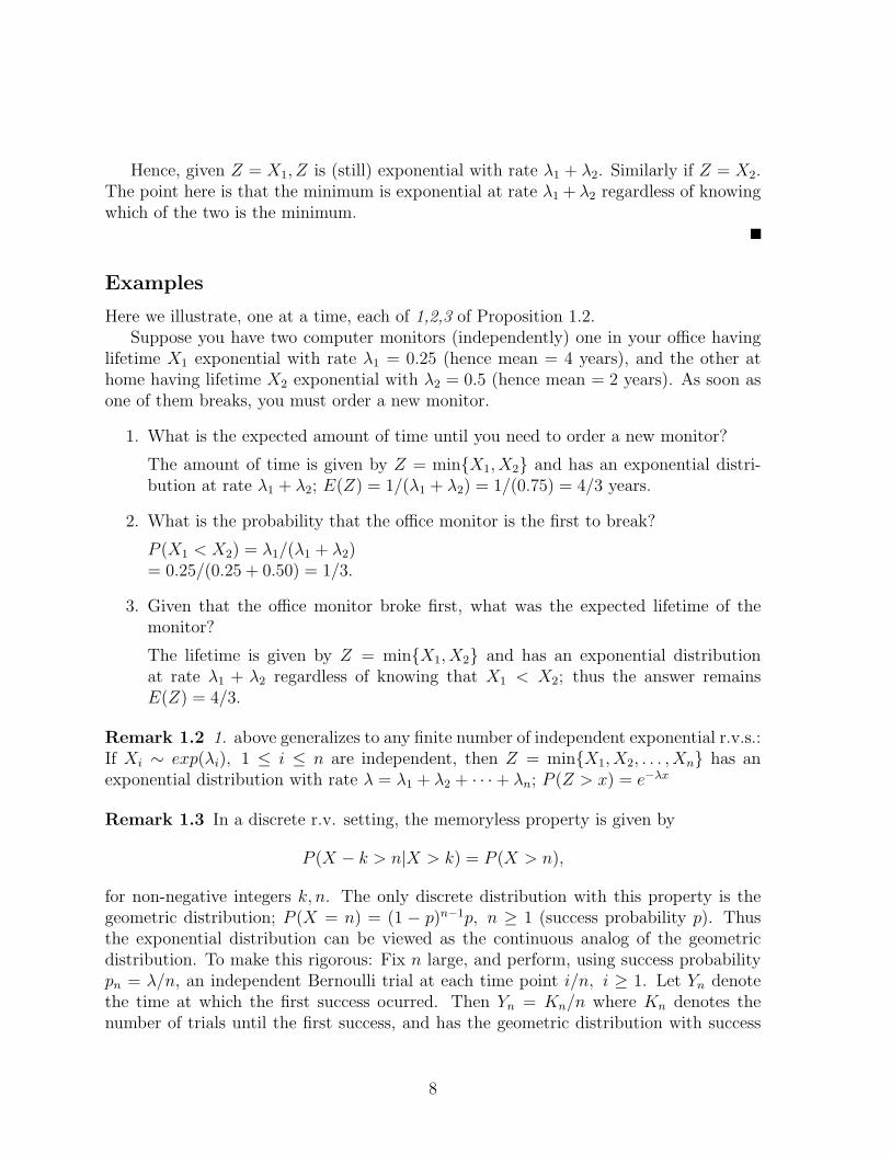
Hence, given Z = X1, Z is (still) exponential with rate λ1 + λ2. Similarly if Z = X2.The point here is that the minimum is exponential at rate λ1 + λ2 regardless of knowingwhich of the two is the minimum.

Examples

Here we illustrate, one at a time, each of 1,2,3 of Proposition 1.2.Suppose you have two computer monitors (independently) one in your office having

lifetime X1 exponential with rate λ1 = 0.25 (hence mean = 4 years), and the other athome having lifetime X2 exponential with λ2 = 0.5 (hence mean = 2 years). As soon asone of them breaks, you must order a new monitor.

1. What is the expected amount of time until you need to order a new monitor?

The amount of time is given by Z = min{X1, X2} and has an exponential distri-bution at rate λ1 + λ2; E(Z) = 1/(λ1 + λ2) = 1/(0.75) = 4/3 years.

2. What is the probability that the office monitor is the first to break?

P (X1 < X2) = λ1/(λ1 + λ2)= 0.25/(0.25 + 0.50) = 1/3.

3. Given that the office monitor broke first, what was the expected lifetime of themonitor?

The lifetime is given by Z = min{X1, X2} and has an exponential distributionat rate λ1 + λ2 regardless of knowing that X1 < X2; thus the answer remainsE(Z) = 4/3.

Remark 1.2 1. above generalizes to any finite number of independent exponential r.v.s.:If Xi ∼ exp(λi), 1 ≤ i ≤ n are independent, then Z = min{X1, X2, . . . , Xn} has anexponential distribution with rate λ = λ1 + λ2 + · · ·+ λn; P (Z > x) = e−λx

Remark 1.3 In a discrete r.v. setting, the memoryless property is given by

P (X − k > n|X > k) = P (X > n),

for non-negative integers k, n. The only discrete distribution with this property is thegeometric distribution; P (X = n) = (1 − p)n−1p, n ≥ 1 (success probability p). Thusthe exponential distribution can be viewed as the continuous analog of the geometricdistribution. To make this rigorous: Fix n large, and perform, using success probabilitypn = λ/n, an independent Bernoulli trial at each time point i/n, i ≥ 1. Let Yn denotethe time at which the first success ocurred. Then Yn = Kn/n where Kn denotes thenumber of trials until the first success, and has the geometric distribution with success

8

probability pn. As n→∞, Yn converges in distribution to a r.v. Y having the exponentialdistribution with rate λ:

P (Yn > x) = P (Kn > nx)

= (1− pn)nx

= (1− (λ/n))nx

→ e−λx, n→∞.

1.6 Stationary and independent increments characterization ofthe Poisson process

Suppose that subway arrival times to a given station form a Poisson process at rate λ.If you enter the subway station at time s > 0 it is natural to consider how long youmust wait until the next subway arrives. But tN(s) ≤ s < tN(s)+1; s lies somewherewithin a subway interarrival time. For example if N(s) = 4 then t4 ≤ s < t5 and slies somewhere within the interarrival time X5 = t5 − t4. But since the interarrivaltimes have an exponential distribution, they have the memoryless property and thusyour waiting time, A(s) = tN(s)+1 − s, until the next subway, being the remainder ofan originally exponential r.v., is itself an exponential r.v. and independent of the past:P (A(s) > t) = e−λt, t ≥ 0. Once the next subway arrives (at time tN(s)+1), the futureinterarrival times are i.i.d. exponentials and independent of A(s). But this means thatthe Poisson process, from time s onword is yet again another Poisson process with thesame rate λ; the Poisson process restarts itself from every time s and is independent ofits past.

In terms of the counting process this means that for fixed s > 0, N(s + t) − N(s)(the number of arrivals during the first t time units after time s, the “future”) has thesame distribution as N(t) (the number of arrivals during the first t time units), and isindependent of {N(u) : 0 ≤ u ≤ s} (the counting process up to time s, the “past”).This above discussion illustrates the stationary and independent increments properties ,to be discussed next. It also shows that that {N(t) : t ≥ 0} is a continuous-time Markovprocess: The future {N(s + t) : t > 0}, given the present state N(s), is independent ofthe past {N(u) : 0 ≤ u < s}.

Definition 1.3 A random point process ψ is said to have stationary increments if for allt ≥ 0 and all s ≥ 0 it holds that N(t+s)−N(s) (the number of points in the time interval(s, s+ t]) has a distribution that only depends on t, the length of the time interval.

For any interval I = (a, b], let N(I) = N(b)−N(a) denote the number of points thatfall in the interval. More generally, for any subset A ⊂ R+, let N(A) denote the numberof points that fall in the subset A.

Definition 1.4 ψ is said to have independent increments if for any two non-overlappingintervals of time, I1 and I2, the random variables N(I1) and N(I2) are independent.

9

We conclude from the discussions above thatThe Poisson process has both stationary and independent increments.But what is this distribution of N(t + s) − N(s) that only depends on t, the length

of the interval? We now show that it is Poisson for the Poisson process:

Proposition 1.3 For a Poisson process at rate λ, the distribution of N(t), t > 0, isPoisson with mean λt:

P (N(t) = k) = e−λt(λt)k

k!, k ≥ 0.

In particular, E(N(t)) = λt, V ar(N(t)) = λt, t ≥ 0. Thus by stationary increments,N(s+ t)−N(s) is also Poisson with mean λt:

P (N(s+ t)−N(s) = k) = e−λt(λt)k

k!, s > 0, k ≥ 0,

and E(N(s+ t)−N(s)) = λt, V ar(N(s+ t)−N(s)) = λt, t ≥ 0.

Proof : Note that P (N(t) = n) = P (tn+1 > t)− P (tn > t). We will show that

P (tm > t) = e−λt(1 + λt+ · · ·+ (λt)m−1

(m− 1)!), m ≥ 1, (3)

so that substituting in m = n+ 1 and m = n and subtracting yields the result.To this end, observe that differentiating the tail Qn(t) = P (tn > t) (recall that tn has

the gamma(n, λ) density in (2)) yields

d

dtQn(t) = −fn(t) = −λe−λt (λt)n−1

(n− 1)!, Qn(0) = 1.

Differentiating the right hand side of (3), we see that (3) is in fact the solution (anti-derivative).

Because of the above result, we see that λ = E(N(1)); the arrival rate is theexpected number of arrivals in any length one interval.

Examples

1. Suppose cars arrive to the GW Bridge according to a Poisson process at rate λ =1000 per hour. What is the expected value and variance of the number of cars toarrive during the time interval between 2 and 3 o’clock PM?

E(N(3) − N(2)) = E(N(1)) by stationary increments. E(N(1)) = λ1 = 1000.Variance is the same, V ar(N(1)) = λ1 = 1000.

10

2. (continuation)

What is the expected number of cars to arrive during the time interval between 2and 3 o’clock PM, given that 700 cars already arrived between 9 and 10 o’clockthis morning?

E(N(3) − N(2)|N(10) − N(9) = 700) = E(N(3) − N(2)) = E(N(1)) = 1000by independent and stationary increments: the r.v.s. N(I1) = N(3) − N(2) andN(I2) = N(10)−N(9) are independent.

3. (continuation) What is the probability that no cars will arrive during a given 15minute interval?

P (N(0.25) = 0) = e−λ(0.25) = e−250.

Remarkable as it may seem, it turns out that the Poisson process is com-pletely characterized by stationary and independent increments:

Theorem 1.2 Suppose that ψ is a simple random point process that has both stationaryand independent increments. Then in fact, ψ is a Poisson process. Thus the Poissonprocess is the only simple point process with stationary and independent increments.

Proof : We must show that the interarrival times {Xn : n ≥ 1} are i.i.d. with anexponential distribution. Consider the point process onwards right after its first arrivaltime (stopping time) t1 = X1 = inf{t > 0 : N(t) = 1}; {N(X1 + t) − N(X1) : t ≥ 0}.It has interarrival times {X2, X3, . . .}. By stationary and independent increments, theseinterarrival times must be independent of the “past”, X1, and distributed the sameas X1, X2, . . .; thus X2 must be independent of and identically distributed with X1.Continuing in the same fashion, we see that all the interarrival times {Xn : n ≥ 1} arei.i.d. with the same distribution as X1.

2

Note that

P (X1 > s+ t) = P (N(s+ t) = 0)

= P (N(s) = 0, N(s+ t)−N(s) = 0)

= P (N(s) = 0)P (N(t) = 0) (via independent and stationary increments)

= P (X1 > s)P (X1 > t),

But this implies that X1 has the memoryless property, and thus from Proposition 1.1 itmust be exponentially distributed; P (X1 ≤ t) = 1− e−λt for some λ > 0. Thus ψ formsa renewal process with an exponential interarrival time distribution.

2Let {N(t) : t ≥ 0} denote the counting process. As pointed out earlier, it follows from independentincrements that it satisfies the Markov property, hence is a continuous-time Markov chain with discretestate space the non-negative integers, hence satisfies the strong Markov property.

11

We now have two different ways of identifying a Poisson process: (1) check-ing if it is a renewal process with an exponential interarrival time distribution,or (2) checking if it has both stationary and independent increments.

1.7 Constructing a Poisson process from independent Bernoullitrials, and the Poisson approximation to the binomial dis-tribution

A Poisson process at rate λ can be viewed as the result of performing an independentBernoulli trial with success probability p = λdt in each “infinitesimal” time interval oflength dt, and placing a point there if the corresponding trial is a success (no pointthere otherwise). Intuitively, this would yield a point process with both stationary andindependent increments; a Poisson process: The number of Bernoulli trials that can befit in any interval only depends on the length of the interval and thus the distribution forthe number of successes in that interval would also only depend on the length; stationaryincrements follows. For two non-overlapping intervals, the Bernoulli trials in each wouldbe independent of one another since all the trials are i.i.d., thus the number of successesin one interval would be independent of the number of successes in the other interval;independent increments follows. We proceed next to explain how this Bernoulli trialsidea can be made rigorous.

As explained in Remark 1.2, the exponential distribution can be obtained as a limit ofthe geometric distribution: Fix n large, and perform, using success probability pn = λ/n,an independent Bernoulli trial at each time point i/n, i ≥ 1. Let Yn denote the timeat which the first success ocurred. Then Yn = Kn/n where Kn denotes the number oftrials until the first success, and has the geometric distribution with success probabilitypn. As n → ∞, Yn converges to a r.v. Y having the exponential distribution with rateλ. This Y thus can serve as the first arrival time t1 for a Poisson process at rate λ. Theidea here is that the tiny intervals of length 1/n become (in the limit) the infinitesimal dtintervals. Once we have our first success, at time t1, we continue onwards in time (in theinterval (t1,∞)) with new Bernoulli trials until we get the second success at time t2 andso on until we get all the arrival times {tn : n ≥ 1}. By construction, each interarrivaltime, Xn = tn − tn−1, n ≥ 1, is an independent exponentially distributed r.v. with rateλ; hence we constructed a Poisson process at rate λ.

Another key to understanding how the Poisson process can be constructed fromBernoulli trials is the fact that the Poisson distribution can be used to approximatethe binomial distribution:

Proposition 1.4 For λ > 0 fixed, let X ∼ binomial(n, p) with success probability pn =λ/n. Then, as n→∞, X converges in distribution to a Poisson rv with mean λ. Thus,a binomial distribution in which the number of trials n is large and the success probabilityp is small can be approximated by a Poisson distrbution with mean λ = np.

12

Proof : Since

P (X = k) =

(n

k

)pk(1− p)n−k,

where p = λ/n, we must show that for any k ≥ 0

limn→∞

(n

k

)(λ/n)k(1− λ/n)n−k = e−λ

λk

k!.

re-writing and expanding yields(n

k

)(λ/n)k(1− λ/n)n−k =

n!

nk× λk

k!× (1− λ/n)n

(1− λ/n)k,

the product of three pieces.But limn→∞(1−λ/n)k = 1 since k is fixed, and from calculus, limn→∞(1−λ/n)n = e−λ.

Moreover,n!

nk=n

n× (n− 1)

n× · · · × (n− k + 1)

n,

and hence converges to 1 as n→∞. Combining these facts yields the result.

We can use the above result to construct the counting process at time t, N(t), fora Poisson process as follows: Fix t > 0. Divide the interval (0, t] into n subintervals,((i− 1)t/n, it/n], 1 ≤ i ≤ n, of the equal length t/n. At the right endpoint it/n of eachsuch subinterval, perform a Bernoulli trial with success probability pn = λt/n, and placea point there if successful (no point otherwise). Let Nn(t) denote the number of suchpoints placed (successes). Then Nn(t) ∼ binomial(n, pn) and converges in distribution toN(t) ∼ Poisson(λt), as n→∞. Moreover, the points placed in (0, t] from the Bernoullitrials converge (as n→∞) to the points t1, . . . , tN(t) of the Poisson process during (0, t].So we have actually obtained the Poisson process up to time t.

1.8 Little o(t) results for stationary point processes

Let o(t) denote any function of t that satisfies o(t)/t → 0 as t → 0. Examples includeo(t) = tn, n > 1, but there are many others.

If ψ is any point process with stationary increments and λ = E(N(1)) < ∞, then(see below for a discussion of proofs)

P (N(t) > 0) = λt+ o(t), (4)

P (N(t) > 1) = o(t). (5)

Because of stationary increments we get the same results for any increment of lengtht, N(s+ t)−N(s), and in words (4) can be expressed as

P (at least 1 arrival in any interval of length t) = λt+ o(t),

13

whereas (5) can be expressed as

P (more than 1 arrival in any interval of length t) = o(t).

Since P (N(t) = 1) = P (N(t) > 0)− P (N(t) > 1), (4) and (5) together yield

P (N(t) = 1) = λt+ o(t), (6)

or in wordsP ( An arrival in any interval of length t) = λt+ o(t).

We thus get for any s ≥ 0:

P (N(s+ t)−N(s) = 1) ≈ λt, for t small,

which using infinitesimals can be written as

P (N(s+ dt)−N(s) = 1) = λdt. (7)

The above o(t) results hold for any (simple) point process with stationary increments,not just a Poisson process. But note how (7) agrees with our Bernoulli trials interpreta-tion of the Poisson process, e.g., performing in each interval of length dt an independentBernoulli trial with success probability p = λdt. But the crucial difference is that ourBernoulli trials construction also yields the independent increments property which isnot expressed in (7). This difference helps explain why the Poisson process is the uniquesimple point process with both stationay and independent increments: There are numer-ous examples of point processes with stationary increments (we shall offer some exampleslater), but only one with both stationary and independent increments; the Poisson pro-cess.

Although a general proof of (4) and (5) is beyond the scope of this course, we willbe satisfied with proving it for the Poisson process at rate λ for which it follows directlyfrom the Taylor’s expansion for ex:

P (N(t) > 0) = 1− e−λt

= 1− (1− λt+(λt)2

2+ · · · )

= λt+(λt)2

2+ · · · )

= λt+ o(t).

P (N(t) > 1) = P (N(t) = 2) + P (N(t) = 3) + · · ·

= e−λt((λt)2

2+ · · · )

≤ ((λt)2

2+ · · · )

= o(t)

14

1.9 Partitioning Theorems for Poisson processes and randomvariables

Given X ∼ Poiss(α) (a Poisson rv with mean α) suppose that we imagine that X denotessome number of objects (arrivals during some fixed time interval for example), and thatindependent of one another, each such object is of type 1 or type 2 with probability pand q = 1 − p respectively. This means that if X = n then the number of those n thatare of type 1 has a binomial(n, p) distribution and the number of those n that are oftype 2 has a binomial(n, q) distribution. Let X1 and X2 denote the number of type 1and type 2 objects respectively ; X1 + X2 = X. The following shows that in fact if wedo this, then X1 and X2 are independent Poisson random variables with means pα andqα respectively.

Theorem 1.3 (Partitioning a Poisson r.v.) If X ∼ Poiss(α) and if each object ofX is, independently, type 1 or type 2 with probability p and q = 1 − p, then in factX1 ∼ Poiss(pα), X2 ∼ Poiss(qα) and they are independent.

Proof : We must show that

P (X1 = k,X2 = m) = e−pα(pα)k

k!e−qα

(qα)m

m!. (8)

P (X1 = k,X2 = m) = P (X1 = k,X = k +m) = P (X1 = k|X = k +m)P (X = k +m).

But given X = k +m, X1 ∼ Bin(k +m, p) yielding

P (X1 = k|X = k +m)P (X = k +m) =(k +m)!

k!m!pkqmeα

αk+m

(k +m)!.

Using the fact that eα = epαeqα and other similar algabraic identites, the above reducesto (8) as was to be shown.

The above theorem generalizes to Poisson processes:

Theorem 1.4 (Partitioning a Poisson process) If ψ ∼ PP (λ) and if each arrivalof ψ is, independently, type 1 or type 2 with probability p and q = 1 − p then in fact,letting ψi denote the point process of type i arrivals, i = 1, 2, ψ1 ∼ PP (pλ), ψ2 ∼ PP (qλ)and they are independent.

Proof : It is immediate that each ψi is a Poisson process since each remains havingstationary and independent increments. Let N(t) and Ni(t), i = 1, 2 denote the cor-responding counting processes, N(t) = N1(t) + N2(t), t ≥ 0. From Theorem 1.3,N1(1) and N2(1) are independent Poisson rvs with means E(N1(1)) = λ1 = pλ and

15

E(N1(1)) = λ2 = qλ since they are a partitioning of N(1); thus πi indeed has rateλi, i = 1, 2. What remains to show is that the two counting processes (as processes) areindependent. But this is immediate from Theorem 1.3 and independent increments ofψ: If we take any collection of non-overlapping intervals (sets more generally) A1, . . . Akand non-overlapping intervals B1, . . . Bl then we must show that (N1(A1), . . . , N1(Ak))is independent of (N2(B1), . . . , N2(Bl)) argued as follows: Any part (say subset C) ofthe Ai which intersect with the Bi will yield independence due to partitioning of the rvN(C), and any parts of the Ai that are disjoint from the Bi will yield independence dueto the independent increments of ψ; thus independence follows.

The above is quite interesting for it means that if Poisson arrivals at rate λ come toour lecture room, and upon each arrival we flip a coin (having probability p of landingheads), and route all those for which the coin lands tails (type 2) into a different room,only allowing those for which the coin lands heads (type 1) enter our room, then thearrival processes to the two room are independent and Poisson.

For example, suppose that λ = 30 per hour, and p = 0.6. Letting N1(t) and N2(t)denote the counting processes for type 1 and type 2 respectively, this means that N1(t) ∼Poiss(α) where α = (0.6)(30)(t) = 18t. Now consider the two events

A = {5 arrivals into room 1 during the hours 1 to 3}

andB = {1000 arrivals into room 2 during the hours 1 to 3}.

We thus conclude that the two events A and B are independent yielding

P (A|B) = P (A)

= P (N1(3)−N1(1) = 5)

= P (N1(2) = 5)

= e−36 365

5!.

In the above computation, the third equality follows from stationary increments (of type1 arrivals since they are Poisson at rate 18).

1.9.1 Supersposition of independent Poisson processes

In the previous section we saw that a Poisson process ψ can be partitioned into twoindependent ones ψ1 and ψ2 (type 1 and type 2 arrivals). But this means that they canbe put back together again to obtain ψ. Putting together means taking the superpositionof the two point processes, that is, combining all their points together, then placing themin acsending order, to form one point process ψ (regardless of type). We write this asψ = ψ1 + ψ2, and of course we in particular have N(t) = N1(t) +N2(t), t ≥ 0.

16

A little thought reveals that therefore we can in fact start with any two independentPoisson processes, ψ1 ∼ PP (λ1), ψ2 ∼ PP (λ2) (call them type 1 and type 2) andsuperpose them to obtain a Poisson process ψ = ψ1 + ψ2 at rate λ = λ1 + λ2. Thepartitioning probability p is given by

p =λ1

λ1 + λ2

,

because that is the required p which would allow us to partition a Poisson process withrate λ = λ1 + λ2 into two independent Poisson processes at rate λ1 and λ2; λp = λ1 andλ(1 − p) = λ2 as is required. p is simply the probability that (starting from any timet) the next arrival time of type 1 (call this Y1) ocurrs before the next arrival time oftype 2 (call this Y2), which by the memoryless proberty is given by P (Y1 < Y2) = λ1

λ1+λ2

because Y1 ∼ exp(λ1), Y2 ∼ exp(λ2) and they are independent by assumption. Once anarrival ocurrs, the memoryless property allows us to conclude that the next arrival willyet again be of type 1 or 2 (independent of the past) dependening only on which of twoindependent exponenialy distributed r.v.s. is smaller; P (Y1 < Y2) = λ1

λ1+λ2. Continuing in

this fashion we conclude that indeed each arrival from the superposition ψ is, independentof all others, of type 1 or type 2 with probability p = λ1

λ1+λ2.

Arguing directly that the superposition of independent Poisson processes yields a Pois-son process is easy: The superposition has both stationary and independent increments,and thus must be a Poisson process. Moreover E(N(1)) = E(N1(1))+E(N2(1)) = λ1+λ2,so the rate indeed is given by λ = λ1 + λ2.

Examples

Foreign phone calls are made to your home phone according to a Poisson process at rateλ1 = 2 (per hour). Independently, domestic phone calls are made to your home phoneaccording to a Poisson process at rate λ2 = 5 (per hour).

1. You arrive home. What is the probability that the next call will be foreign? Thatthe next three calls will be domestic?

Answers: λ1

λ1+λ2= 2/7, ( λ2

λ1+λ2)3 = (5/7)3. Once a domestic call comes in, the

future is independent of the past and has the same distribution as when we startedby the memoryless property, so the next call will, once again be domestic with thesame probability 5/7 and so on.

2. You leave home for 2 hours. What is the mean and variance of the number of callsyou recieved during your absence?

Answer: The superposition of the two types is a Poisson process at rate λ =λ1 +λ2 = 7. Letting N(t) denote the number of calls by time t, it follows that N(t)has a Poisson distribution with parameter λt; E(N(2)) = 2λ = 14 = V ar(N(2)).

17

3. Given that there were exactly 5 calls in a given 4 hour period, what is the probabilitythat exactly 2 of them were foreign?

Answer: The superposition of the two types is a Poisson process at rate λ =λ1 + λ2 = 7. The individual foriegn and domestic arrival processes can be viewedas type 1 and 2 of a partitioning with p = λ1

λ1+λ2= 2/7. Thus given N(4) = 5,

the number of those 5 that are foriegn (type 1) has a Bin(5, p) distribution. withp = 2/7. Thus we want (

5

2

)p2(1− p)3.

1.10 Constructing a Poisson process up to time t by using theorder statistics of iid uniform rvs

Suppose that for a Poisson process at rate λ, we condition on the event {N(t) = 1}, theevent that exactly one arrival ocurred during (0, t]. We might conjecture that under suchconditioning, t1 should be uniformly distributed over (0, t). To see that this is in fact so,choose s ∈ (0, t). Then

P (t1 ≤ s|N(t) = 1) =P (t1 ≤ s,N(t) = 1)

P (N(t) = 1)

=P (N(s) = 1, N(t)−N(s) = 0)

P (N(t) = 1)

=e−λsλse−λ(t−s)

e−λtλt

=s

t.

It turns out that this result generalizes nicely to any number of arrivals, and wepresent this next.

Let U1, U2, . . . , Un be n i.i.d uniformly distributed r.v.s. on the interval (0, t). LetU(1) < U(2) < · · · < U(n) denote them placed in ascending order. Thus U(1) is the smallestof them , U(2) the second smallest and finally U(n) is the largest one. U(i) is called the ith

order statistic of U1, . . . Un.Note that the joint density function of (U1, U2, . . . , Un) is given by

g(s1, s2, . . . , sn) =1

tn, si ∈ (0, t),

because each Ui has density function 1/t and they are independent. Now given anyascending sequence 0 < s1 < s2 < · · · < sn < t it follows that the joint distributionf(s1, s2, . . . , sn) of the order statistics (U(1), U(2), . . . , U(n)) is given by

f(s1, s2, . . . , sn) =n!

tn,

18

because there are n! permutations of the sequence (s1, s2, . . . , sn) each of which leadsto the same order statistics. For example if (s1, s2, s3) = (1, 2, 3) then there are 3! = 6permutations all yielding the same order statistics (1, 2, 3): (1, 2, 3), (1, 3, 2), (2, 1, 3),(2, 3, 1), (3, 1, 2), (3, 2, 1).

Theorem 1.5 For any Poisson process, conditional on the event {N(t) = n}, the jointdistribution of the n arrival times t1, . . . , tn is the same as the joint distribution ofU(1), . . . , U(n), the order statistics of n i.i.d. unif(0, t) r.v.s., that is, it is given by

f(s1, s2, . . . , sn) =n!

tn, 0 < s1 < s2 < · · · < sn < t

Proof : We will compute the density for

P (t1 = s1, . . . , tn = sn|N(t) = n) =P (t1 = s1, . . . , tn = sn, N(t) = n)

P (N(t) = n)

and see that it is precisely n!tn

. To this end, we re-write the event {t1 = s1, . . . , tn =sn, N(t) = n} in terms of the i.i.d. interarrival times as {X1 = s1, . . . , Xn = sn −sn−1, Xn+1 > t−sn}. For example if N(t) = 2, then {t1 = s1, t2 = s2, N(t) = 2} = {X1 =s1, X2 = s2 − s1, X3 > t − s2} and thus has density λe−λs1λe−λ(s2−s1)e−λ(t−s2) = λ2e−λt

due to the independence of the r.v.s. X1, X2, X3, and the algebraic cancellations in theexponents.

We conclude that

P (t1 = s1, . . . , tn = sn|N(t) = n) =P (t1 = s1, . . . , tn = sn, N(t) = n)

P (N(t) = n)

=P (X1 = s1, . . . , Xn = sn − sn−1, Xn+1 > t− sn)

P (N(t) = n)

=λne−λt

P (N(t) = n)

=n!

tn,

where the last equality follows since P (N(t) = n) = e−λt(λt)n/n!.

The importance of the above is this: If you want to simulate a Poisson process up totime t, you need only first simulate the value of N(t), then if N(t) = n generate n i.i.d.Unif(0, t) numbers (U1, U2, . . . , Un), place them in ascending order (U(1), U(2), . . . , U(n))and finally define ti = U(i), 1 ≤ i ≤ n.

Uniform numbers are very easy to generate on a computer and so this method canhave computational advantages over simply generating exponential r.v.s. for interarrival

19

times Xn, and defining tn = X1 + · · ·+Xn. Exponential r.v.s. require taking logarithmsto generate:

Xi = −1

λlog(Ui),

where Ui ∼ Unif(0, 1) and this can be computationally time consuming.

1.11 Applications

1. A bus platform is now empty of passengers, and the next bus will depart in tminutes. Passengers arrive to the platform according to a Poisson process at rateλ. What is the average waiting time of an arriving passenger?

Answer: Let {N(t)} denote the counting process for passenger arrivals. GivenN(t) = n ≥ 1, we can treat the n passenger arrival times t1, . . . , tn as the orderstatistics U(1) < U(2) < · · · < U(n) of n independent unif(0, t) r.v.s., U1, U2, . . . , Un.

We thus expect that on average a customer waits E(U) = t/2 units of time. Thisindeed is so, proven as follows: The ith arrival has waiting time Wi = t − ti, andthere will be N(t) such arrivals. Thus we need to compute E(T ) where

T =1

N(t)

N(t)∑i=1

(t− ti).

(We only consider the case when N(t) ≥ 1.)

But given N(t) = n, we conclude that

T =1

n

n∑i=1

(t− U(i))

=1

n

n∑i=1

(t− Ui),

because the sum of all n of the U(i) is the same as the sum of all n of the Ui. Thus

E(T |N(t) = n)) =1

nnE(t− U) = E(t− U) =

t

2.

This being true for all n ≥ 1, we conclude that E(T ) = t2.

2. M/GI/∞ queue: Arrival times tn form a Poisson process at rate λ with countingprocess {N(t)}, service times Sn are i.i.d. with general distribution G(x) = P (S ≤x) and mean 1/µ. There are an infinite number of servers and so there is no delay:the nth customer arrives at time tn, enters service immediately at any free serverand then departs at time tn + Sn; Sn is the length of time the customer spends inservice. Let X(t) denote the number of customers in service at time t. We assumethat X(0) = 0.

We will now show that

20

Proposition 1.5 For every fixed t > 0, the distribution of X(t) is Poisson withparameter α(t) where

α(t) = λ

∫ t

0

P (S > x)dx,

P (X(t) = n) = e−α(t) (α(t))n

n!, n ≥ 0.

Thus E(X(t) = α(t) = V ar(X(t)). Moreover since α(t) converges (as t→∞) to

λ

∫ ∞0

P (S > x)dx = λE(S) =λ

µ,

we conclude that

limt→∞

P (X(t) = n) = e−ρρn

n!, n ≥ 0,

where ρ = λ/µ. So the limiting (or steady-state, or stationary) distribution of X(t)exists and is Poisson with parameter ρ.

Proof : The method of proof is actually based on partitioning the Poisson randomvariable N(t) into two types: those that are in service at time t, X(t), and thosethat have departed by time t (denoted by D(t)). Thus we need only figure outwhat is the probability p(t) that a customer who arrived during (0, t] (that is, oneof the N(t) arrivals) is still in service at time t.

We first recall that conditional on N(t) = n the n (unordered) arrival times arei.i.d. with a Unif(0, t) distribution. Letting U denote a typical such arrival time,and S their service time, we conclude that this customer will still be in service attime t if and only if U + S > t (arival time + service time > t); S > t− U . Thusp(t) = P (S > t − U), where S and U are assumed independent. But (as is easilyshown)) t−U ∼ Unif(0, t) if U ∼ Unif(0, t). Thus p = P (S > t−U) = P (S > U).Noting that P (S > U |U = x) = P (S > x) we conclude that

p(t) = P (S > U) =1

t

∫ t

0

P (S > x)dx,

where we have conditioned on the value of U = x (with density 1/t) and integratedover all such values. This did not depend upon the value n and so we are done.

Thus for fixed t, we can partition N(t) into two independent Poisson r.v.s., X(t)and D(t) (the number of departures by t), to conclude that X(t) ∼ Poiss(α(t))where

α(t) = λtp(t) = λ

∫ t

0

P (S > x)dx

as was to be shown. Similarly D(t) ∼ Poisson(β(t)) where β(t) = λt(1−p(t)).

21

Recall that

pjdef= lim

t→∞P (X(t) = j) = e−ρ

ρj

j!,

that is, that the limiting (or steady-state or stationary) distribution of X(t) isPoisson with mean ρ. Keep in mind that this implies convergence in a time averagesense also:

pj = limt→∞

1

t

∫ t

0

P (X(s) = j)ds = e−ρρj

j!,

which is exactly the continuous time analog of the stationary distribution π forMarkov chains:

πj = limn→∞

1

n

n∑k=1

P (Xk = j).

Thus we interpret pj as the long run proportion of time that there are j busyservers. The average number of busy severs is given by the mean of the limitingdistribution:

L =∞∑j=0

jpj = ρ.

Finally note that the mean ρ agrees with our “Little’s Law” (L = λw) derivationof the time average number in system:

L = limt→∞

1

t

∫ t

0

X(s)ds = ρ.

Customers arrival at rate λ and have an average sojourn time of 1/µ yielding L = ρ.In short, the time average number in system is equal to the mean of the limitingdistribution {pj} for number in system.

Final comment: In proving Proposition 1.5, as with the Example 1, we do need touse the fact that summing up over all the order statistics is the same as summing upover the non ordered uniforms. When N(t) = n, we have

X(t) =n∑j=1

I{Sj > t− U(j)}.

But since service times are i.i.d. and independent of the uniforms, we see that this is thesame in distrubtion as the sum

n∑j=1

I{Sj > t− Uj}.

Since the I{Sj > t− Uj} are i.i.d. Bernoulli(p) r.v.s. with p = P (S > U), we concludethat the conditional distribution of X(t) given that N(t) = n, is binomial with successprobability p. Thus X(t) indeed can be viewed as a partitioned N(t) with partitionprobability p = P (S > U).

22

Example

Suppose people in NYC buy advance tickets to a movie according to a Poisson processat rate λ = 500 (per day), and that each buyer independent of all others keeps the ticket(before using) for an amount of time that is distributed as G(x) = P (S ≤ x) = x/4, x ∈(0, 4) (days), the uniform distribution over (0, 4). Assuming that no one owns a ticket attime t = 0, what is the expected number of ticket holders at time t = 2 days? 5 days?,5 years?

Answer: we want E(X(2)) = α(2) and E(X(5)) = α(5) and E(X(5×360)) = α(1800)for the M/G/∞ queue in which

α(t) = 500

∫ t

0

P (S > x)dx.

Here P (S > x) = 1− x/4, x ∈ (0, 4) but P (S > x) = 0, x ≥ 4. Thus

α(2) = 500

∫ 2

0

(1− x/4)dx = 500(3/2) = 750,

and

α(5) = α(1800)) = 500

∫ 4

0

(1− x/4)dx = 500E(S) = 500(2) = 1000.

The point here is that α(t) = λE(S) = ρ = 1000, t ≥ 4: From time t = 4 (days) owards,the limiting distribution is already reached (no need to take the limit t → ∞). It isPoisson with mean ρ = 1000; the distribution of X(t) at time t = 5 days is the same asat time t = 5 years.

If S has an exponential distribution with mean 2 (days), P (S > x) = .5e−.5x, x ≥ 0,then the answers to the above questions would change. In this case

α(t) = 500

∫ t

0

.5e−.5xdx = 1000(1− e−.5t), t ≥ 0.

The limiting distribution is the same, (Poisson with mean ρ = 1000) but we need to takethe limit t→∞ to reach it.

23