1

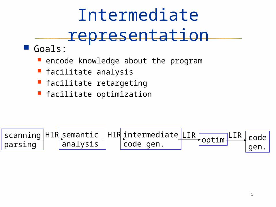
Intermediate representation Goals:

encode knowledge about the program facilitate analysis facilitate retargeting facilitate optimization

scanningparsing

semantic analysis

HIR intermediatecode gen.

HIRoptim

LIR codegen.

LIR

2

Intermediate representation Components

code representation symbol table analysis information string table

Issues Use an existing IR or design a new one? How close should it be to the source/target?

3

IR selection

Using an existing IR cost savings due to reuse it must be expressive and appropriate for the

compiler operations

Designing an IR decide how close to machine code it should be decide how expressive it should be decide its structure consider combining different kinds of IRs

4

IR classification: Level

High-level closer to source language used early in the process usually converted to lower form later on Example: AST

5

IR classification: Level

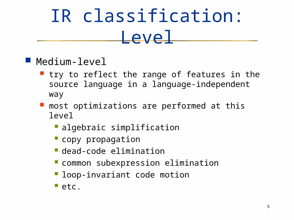
Medium-level try to reflect the range of features in the source

language in a language-independent way most optimizations are performed at this level

algebraic simplification copy propagation dead-code elimination common subexpression elimination loop-invariant code motion etc.

6

IR classification: Level

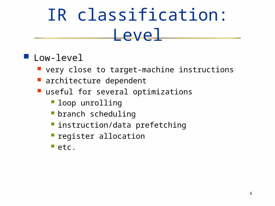
Low-level very close to target-machine instructions architecture dependent useful for several optimizations

loop unrolling branch scheduling instruction/data prefetching register allocation etc.

7

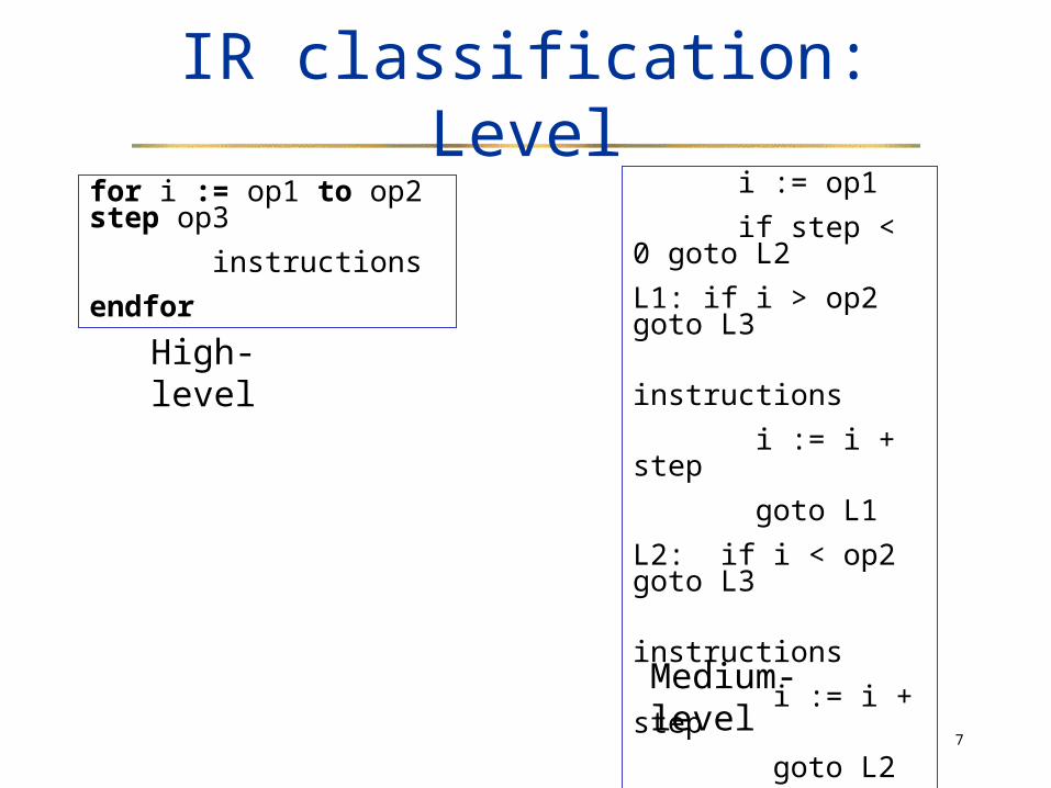
IR classification: Levelfor i := op1 to op2 step op3

instructions

endfor

i := op1

if step < 0 goto L2

L1: if i > op2 goto L3

instructions

i := i + step

goto L1

L2: if i < op2 goto L3

instructions

i := i + step

goto L2

L3:

High-level

Medium-level

8

IR classification: Structure

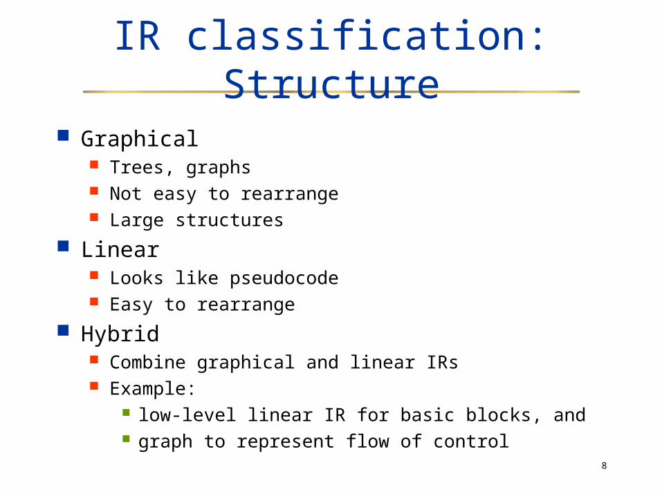
Graphical Trees, graphs Not easy to rearrange Large structures

Linear Looks like pseudocode Easy to rearrange

Hybrid Combine graphical and linear IRs Example:

low-level linear IR for basic blocks, and graph to represent flow of control

9

Graphical IRs

Parse tree Abstract syntax tree

High-level Useful for source-level information Retains syntactic structure Common uses

source-to-source translation semantic analysis syntax-directed editors

10

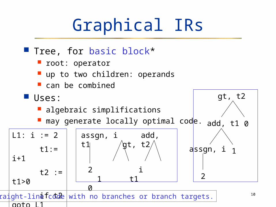
Graphical IRs Tree, for basic block*

root: operator up to two children: operands can be combined

Uses: algebraic simplifications may generate locally optimal code.

L1: i := 2

t1:= i+1

t2 := t1>0

if t2 goto L1

assgn, i add, t1 gt, t2

2 i 1 t1 02

assgn, i 1

add, t1 0

gt, t2

*straight-line code with no branches or branch targets.

11

Graphical IRs

Directed acyclic graphs (DAGs) Like compressed trees

leaves: variables, constants available on entry internal nodes: operators

annotated with variable names? distinct left/right children

Used for basic blocks (DAGs don't show control flow) Can generate efficient code.

Note: DAGs encode common expressions But difficult to transform Good for analysis

12

Graphical IRs

Generating DAGs Check whether an operand is already present

if not, create a leaf for it Check whether there is a parent of the operand that

represents the same operation if not create one, then label the node

representing the result with the name of the destination variable, and remove that label from all other nodes in the DAG.

13

Graphical IRs

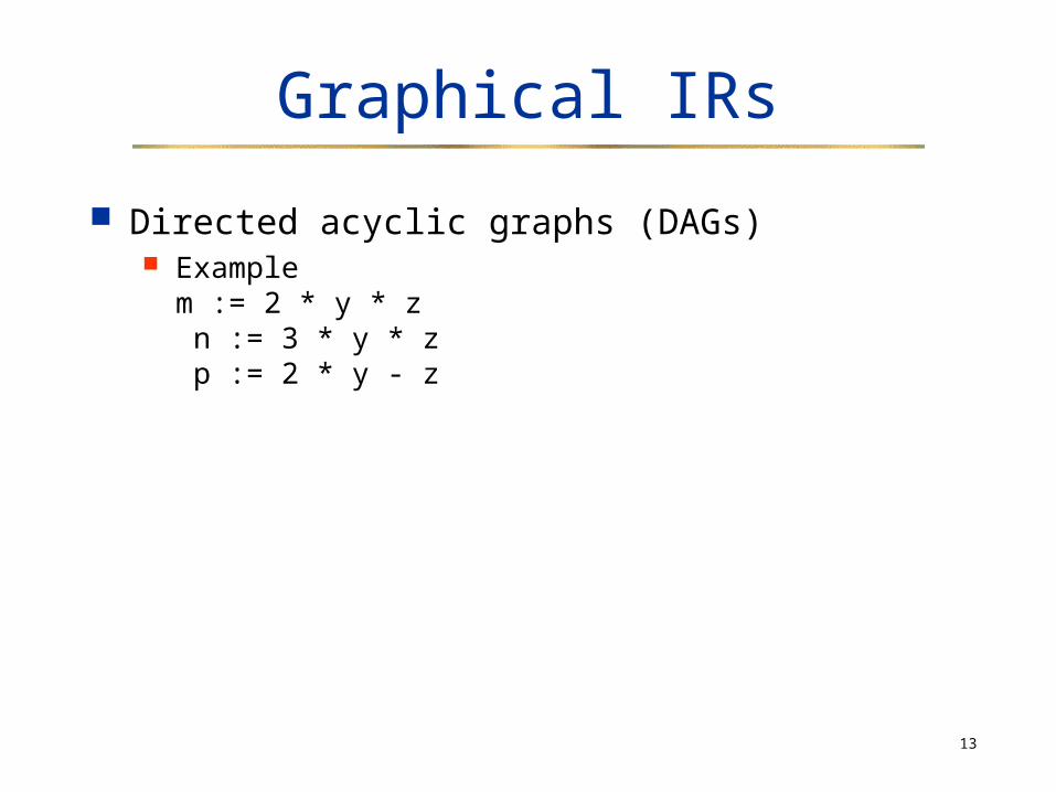
Directed acyclic graphs (DAGs) Example

m := 2 * y * z n := 3 * y * z p := 2 * y - z

14

Graphical IRs

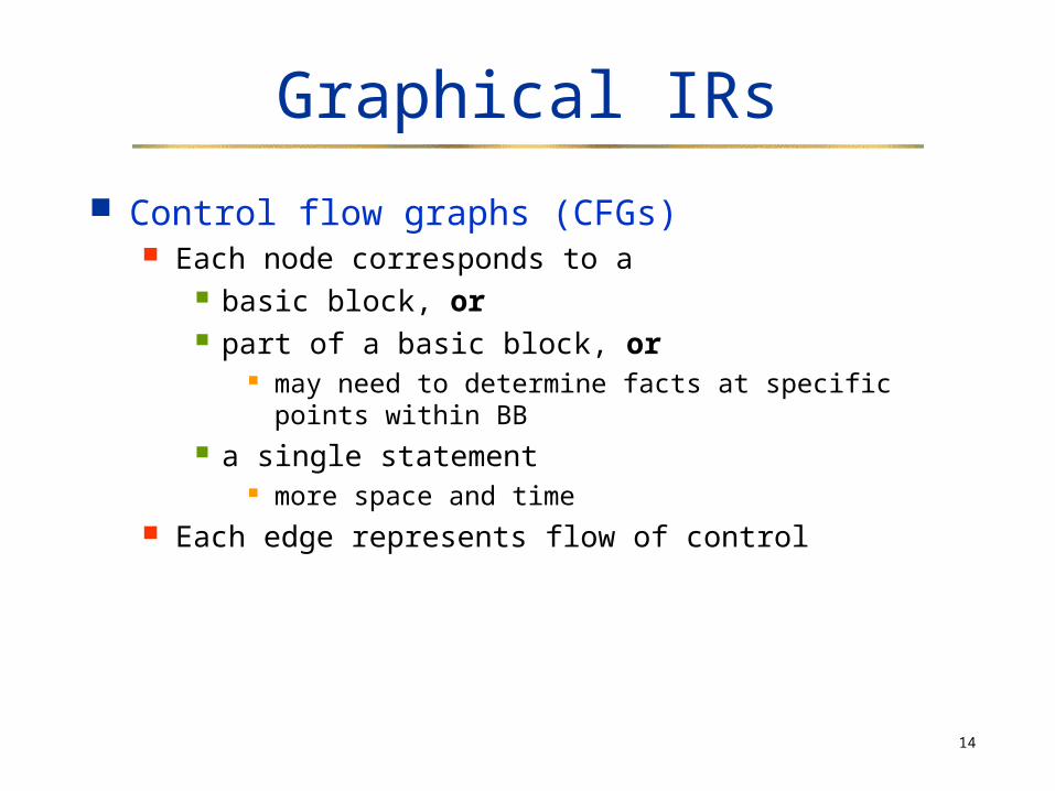
Control flow graphs (CFGs) Each node corresponds to a

basic block, or part of a basic block, or

may need to determine facts at specific points within BB

a single statement more space and time

Each edge represents flow of control

15

Graphical IRs

Dependence graphs : they represents constraints on the sequencing of operations

Dependence = a relation between two statements that puts a constraint on their execution order.

Control dependence Based on the program's control flow.

Data dependence Based on the flow of data between statements.

Nodes represent statements Edges represent dependences

Labels on the edges represent types of dependences Built for specific optimizations, then discarded

16

Graphical IRs

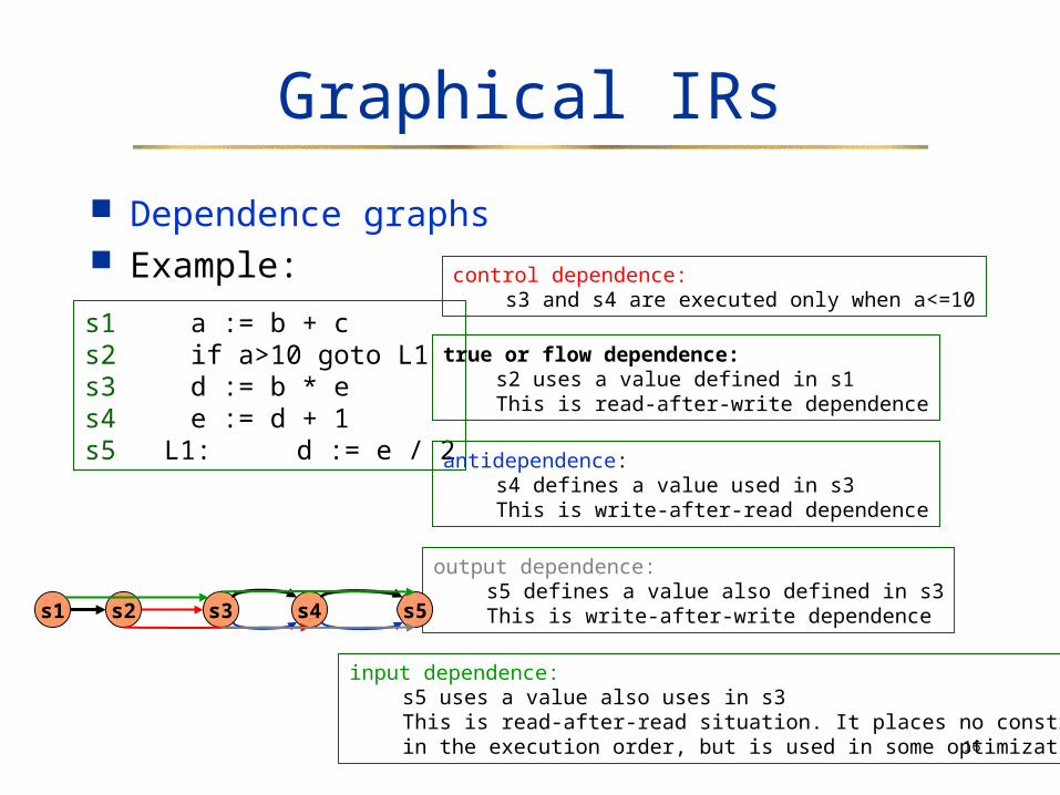
Dependence graphs Example:

s1 a := b + cs2 if a>10 goto L1s3 d := b * es4 e := d + 1s5 L1: d := e / 2

control dependence: s3 and s4 are executed only when a<=10

true or flow dependence: s2 uses a value defined in s1This is read-after-write dependence

antidependence: s4 defines a value used in s3This is write-after-read dependence

output dependence: s5 defines a value also defined in s3This is write-after-write dependence

input dependence: s5 uses a value also uses in s3This is read-after-read situation. It places no constraintsin the execution order, but is used in some optimizations.

s1 s2 s3s4

s5

17

Basic blocks

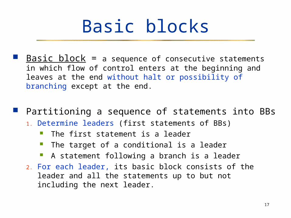
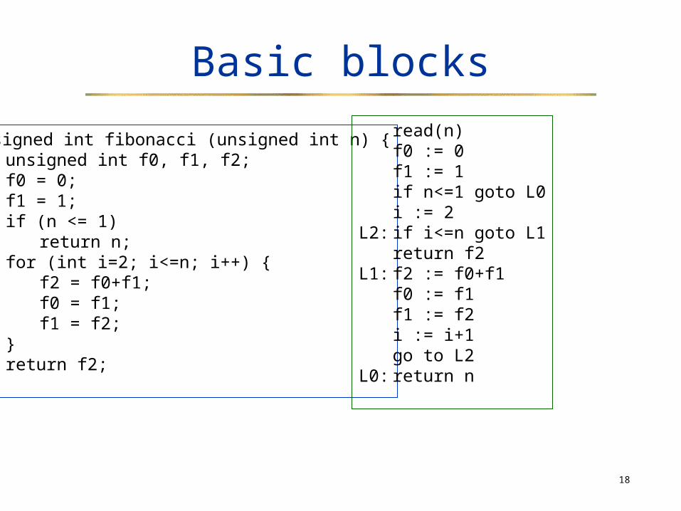
Basic block = a sequence of consecutive statements in which flow of control enters at the beginning and leaves at the end without halt or possibility of branching except at the end.

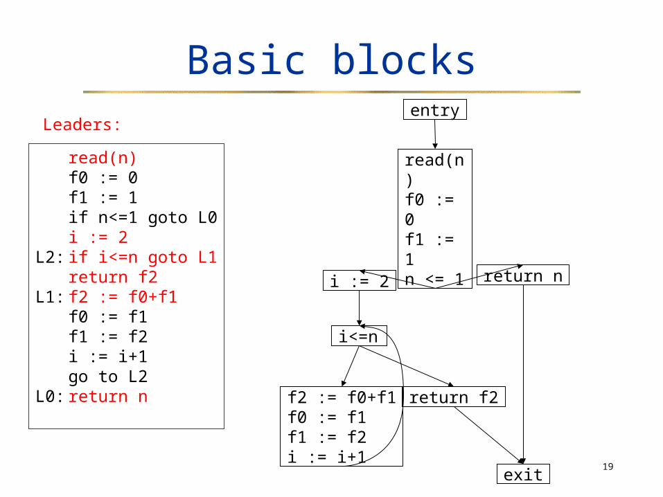
Partitioning a sequence of statements into BBs1. Determine leaders (first statements of BBs)

The first statement is a leader The target of a conditional is a leader A statement following a branch is a leader

2. For each leader, its basic block consists of the leader and all the statements up to but not including the next leader.

18

Basic blocks

unsigned int fibonacci (unsigned int n) {unsigned int f0, f1, f2;f0 = 0;f1 = 1;if (n <= 1)

return n;for (int i=2; i<=n; i++) {

f2 = f0+f1;f0 = f1;f1 = f2;

}return f2;

}

read(n)f0 := 0f1 := 1if n<=1 goto L0i := 2

L2: if i<=n goto L1return f2

L1: f2 := f0+f1f0 := f1f1 := f2i := i+1go to L2

L0: return n

19

Basic blocks

read(n)f0 := 0f1 := 1if n<=1 goto L0i := 2

L2: if i<=n goto L1return f2

L1: f2 := f0+f1f0 := f1f1 := f2i := i+1go to L2

L0: return n

Leaders:

read(n)f0 := 0f1 := 1n <= 1

i := 2

i<=n

return f2f2 := f0+f1f0 := f1f1 := f2i := i+1

return n

exit

entry

20

Linear IRs

Sequence of instructions that execute in order of appearance

Control flow is represented by conditional branches and jumps

Common representations stack machine code three-address code

21

Linear IRs

Stack machine code Assumes presence of operand stack Useful for stack architectures, JVM Operations typically pop operands and push results. Advantages

Easy code generation Compact form

Disadvantages Difficult to rearrange Difficult to reuse expressions

22

Linear IRs

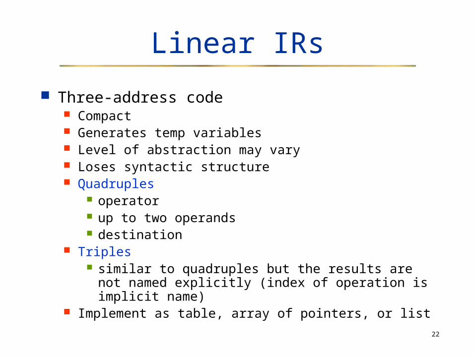
Three-address code Compact Generates temp variables Level of abstraction may vary Loses syntactic structure Quadruples

operator up to two operands destination

Triples similar to quadruples but the results are not

named explicitly (index of operation is implicit name)

Implement as table, array of pointers, or list

23

Linear IRs

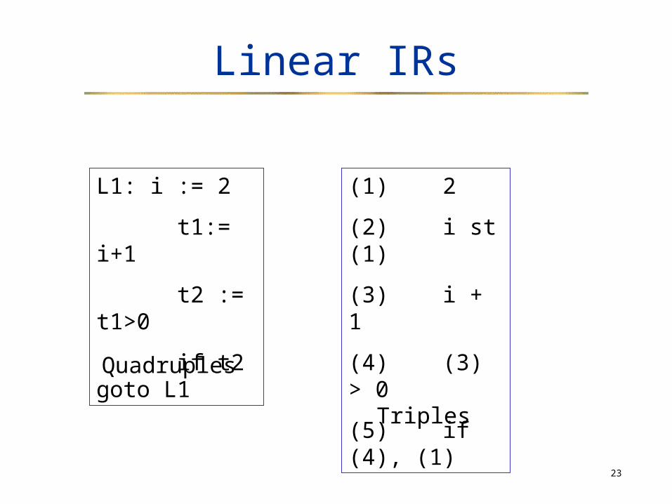
L1: i := 2

t1:= i+1

t2 := t1>0

if t2 goto L1

(1) 2

(2) i st (1)

(3) i + 1

(4) (3) > 0

(5) if (4), (1)Quadruples

Triples

24

SSA form

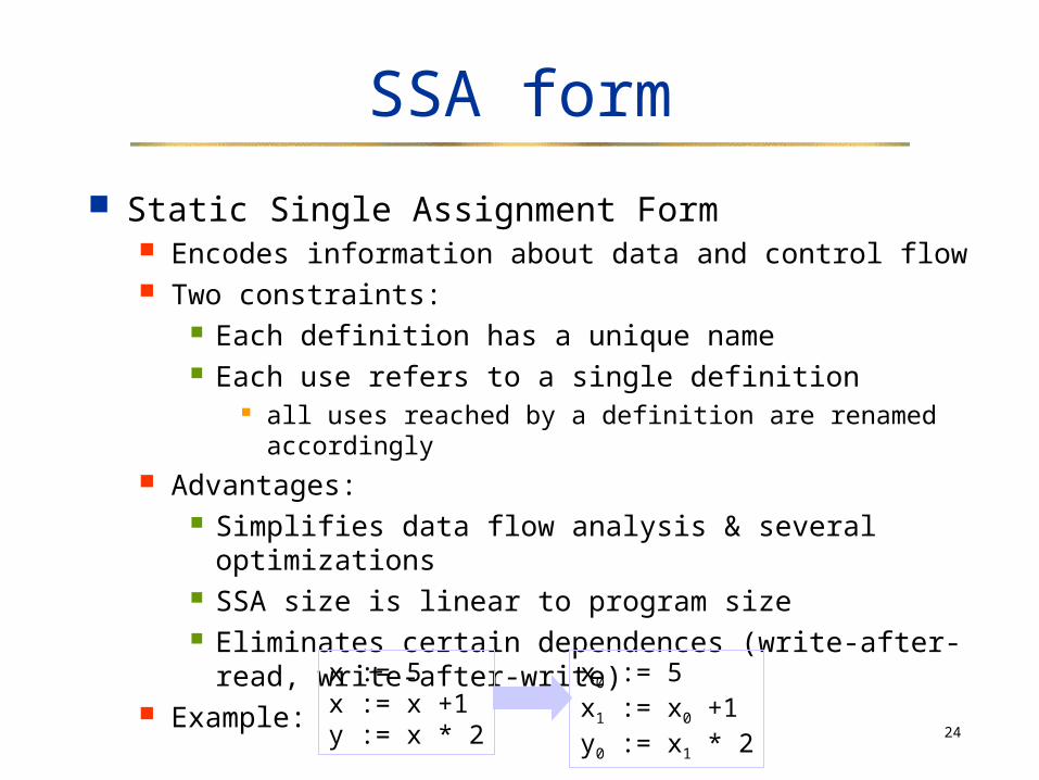
Static Single Assignment Form Encodes information about data and control flow Two constraints:

Each definition has a unique name Each use refers to a single definition

all uses reached by a definition are renamed accordingly

Advantages: Simplifies data flow analysis & several

optimizations SSA size is linear to program size Eliminates certain dependences (write-after-read,

write-after-write) Example:

x := 5x := x +1y := x * 2

x0 := 5x1 := x0 +1y0 := x1 * 2

25

SSA form

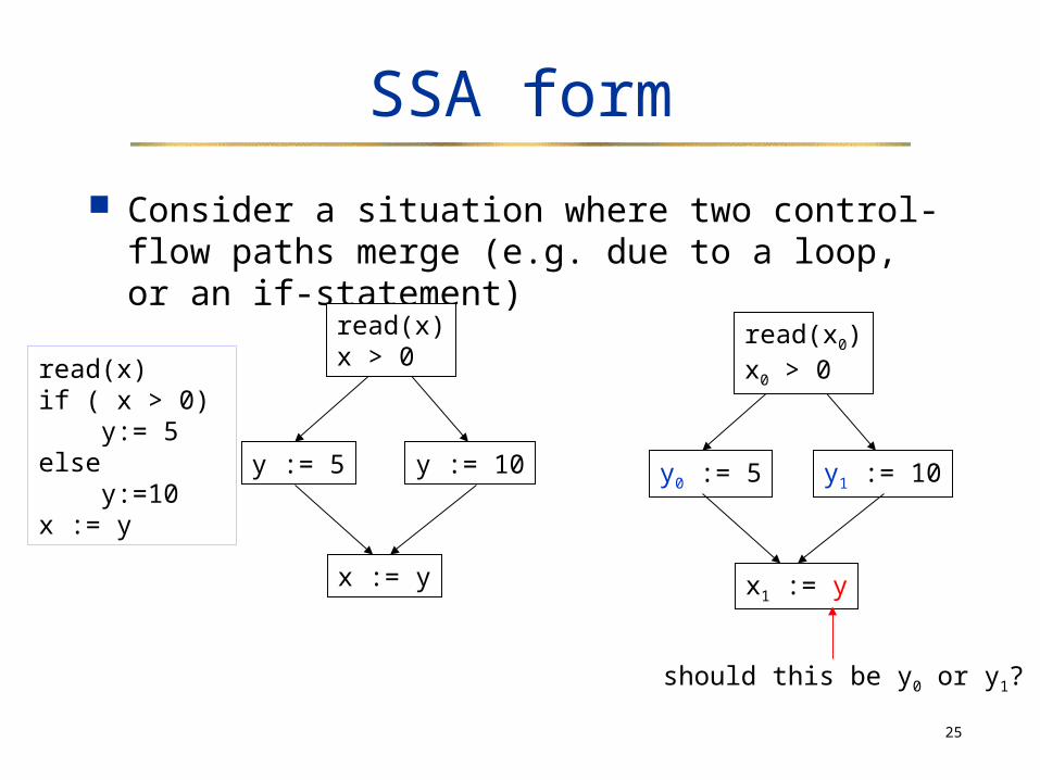
Consider a situation where two control-flow paths merge (e.g. due to a loop, or an if-statement)

read(x)if ( x > 0) y:= 5else y:=10x := y

y := 5 y := 10

x := y

read(x)x > 0

y0 := 5 y1 := 10

x1 := y

read(x0)x0 > 0

should this be y0 or y1?

26

SSA form

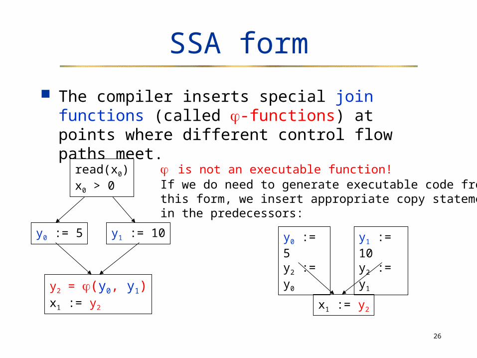
The compiler inserts special join functions (called -functions) at points where different control flow paths meet.

y0 := 5 y1 := 10

y2 = (y0, y1)x1 := y2

read(x0)x0 > 0

is not an executable function!If we do need to generate executable code fromthis form, we insert appropriate copy statementsin the predecessors:

y0 := 5y2 := y0

y1 := 10y2 := y1

x1 := y2

27

SSA form

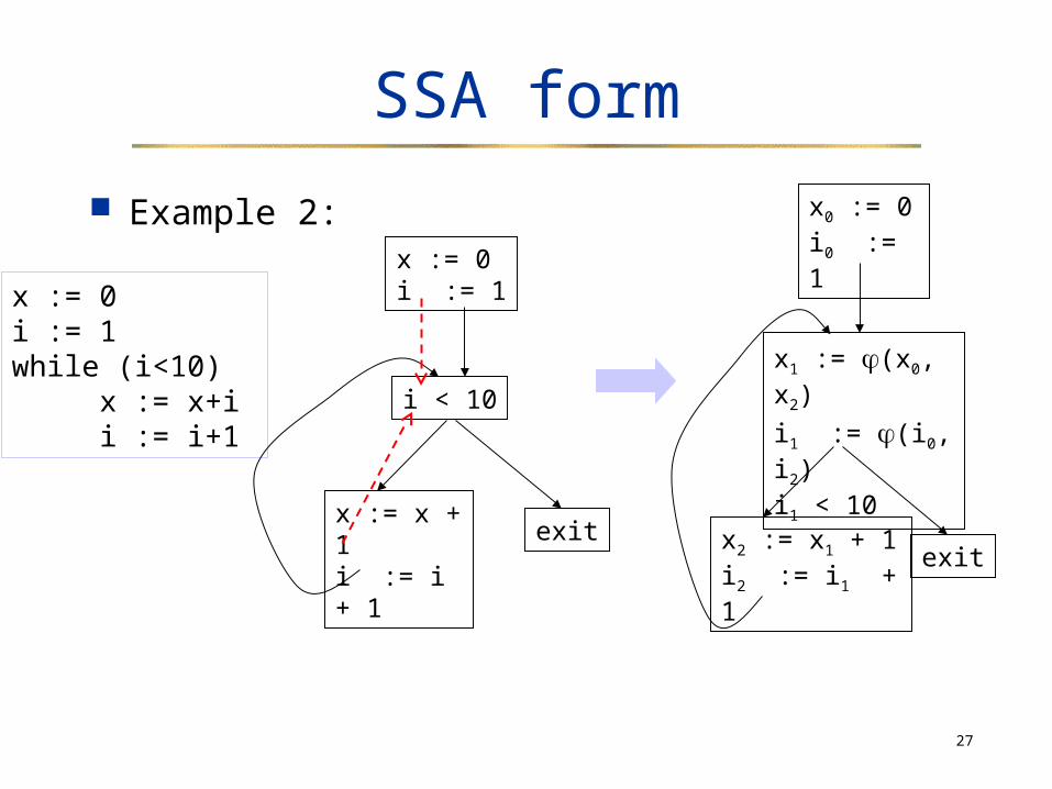
Example 2:

x := 0 i := 1 while (i<10) x := x+i i := i+1

i < 10

exitx := x + 1i := i + 1

x := 0i := 1

x1 := (x0, x2)

i1 := (i0, i2)i1 < 10

exitx2 := x1 + 1i2 := i1 + 1

x0 := 0i0 := 1

28

SSA form

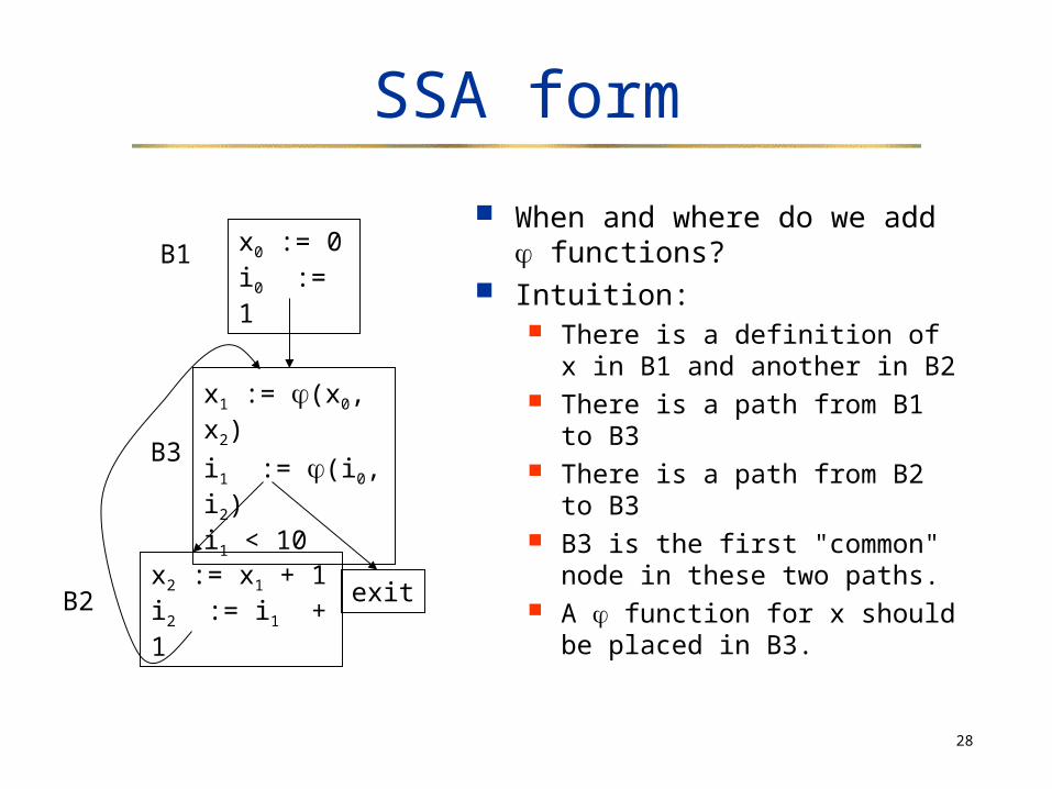
When and where do we add functions?

Intuition: There is a definition of x in B1

and another in B2 There is a path from B1 to B3 There is a path from B2 to B3 B3 is the first "common" node

in these two paths. A function for x should be

placed in B3.

x1 := (x0, x2)

i1 := (i0, i2)i1 < 10

exitx2 := x1 + 1i2 := i1 + 1

x0 := 0i0 := 1

B1

B2

B3

29

SSA form

A program is in SSA form if Each variable is assigned a value in exactly one

statement Each use of a variable is dominated by the definition.

Domination Node A dominates node B if every path from the flow

graph entry to B goes through A Every node dominates itself Intuition: control will have to go through A in order to

reach B

Dominators are useful in identifying loops and in computing the SSA form.

30

Dominators

A node N may have several dominators, but one of them will be closest to N and be dominated by all other dominators of N. That node is called the immediate dominator of N.

The dominator tree is a data structure that shows the dominator relationships of a control flow graph. Each node in the tree is the immediate dominator of

its children.

31

B1

B2

B3

B4

B5 B6

B7

B8

B9

B10

entry

exit

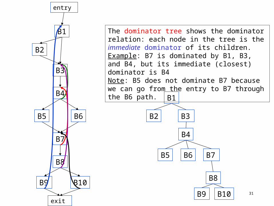
The dominator tree shows the dominator relation: each node in the tree is the immediate dominator of its children.Example: B7 is dominated by B1, B3, and B4, but its immediate (closest) dominator is B4Note: B5 does not dominate B7 because we can go from the entry to B7 through the B6 path.

B1

B2 B3

B4

B5 B6 B7

B8

B9

B10

32

Dominators and loops

We can use dominators to identify the loops in a flow graph:

Natural Loop = A set of basic blocks with a single entry point called the header, which

dominates all other blocks in the set, and at least one way to iterate (i.e. go back to the

header)

Loop-finding algorithm: Find an edge BA where A dominates B. This is

called a back-edge. Add A and B to the loop Find all nodes that can reach B without going

through A. Add them to the loop.

33

Loopsback edge: B9B1loop: {B9, B8, B7, B10, B6, B5, B4, B3, B2, B1}

B1

B2

B3

B4

B5 B6

B7

B8

B9

B10

entry

exit

back edge: B10B7loop: {B10, B8, B7}

back edge: B8B3loop: {B8, B7, B10, B6, B5, B4, B3 }

back edge: B7B4loop: {B7, B10, B6, B5, B8, B4}

back edge: B4B3loop: {B4, B7, B10, B8, B6, B5, B3}

34

Nested Loops

Loop K is nested within loop L if L and K have different headers, and respectively,

and is dominated by

35

Dominators and SSA form

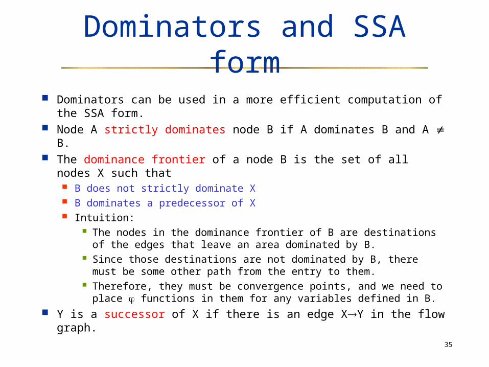
Dominators can be used in a more efficient computation of the SSA form.

Node A strictly dominates node B if A dominates B and A B.

The dominance frontier of a node B is the set of all nodes X such that B does not strictly dominate X B dominates a predecessor of X Intuition:

The nodes in the dominance frontier of B are destinations of the edges that leave an area dominated by B.

Since those destinations are not dominated by B, there must be some other path from the entry to them.

Therefore, they must be convergence points, and we need to place functions in them for any variables defined in B.

Y is a successor of X if there is an edge XY in the flow graph.

36

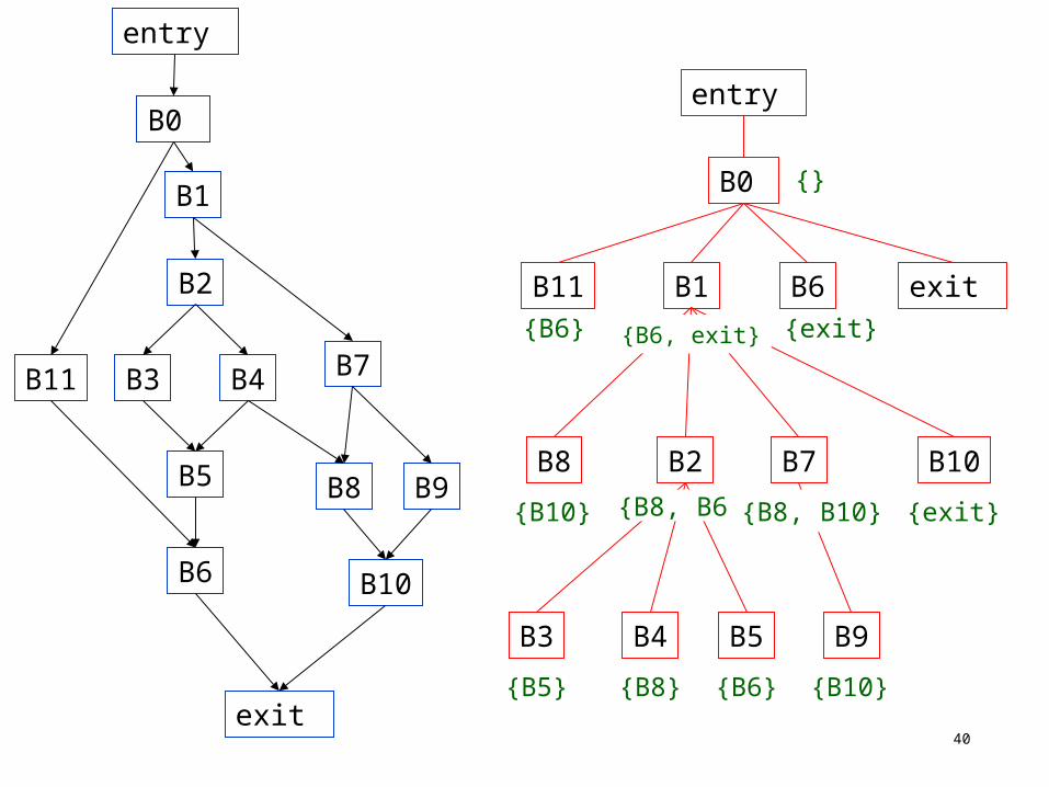
Dominance frontier

B1

B2

B3 B4

B5

B0

B6

B7

B8 B9

B10

B11

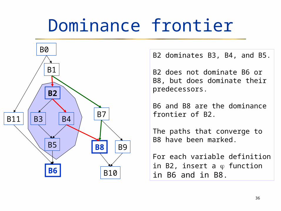
B2 dominates B3, B4, and B5.

B2 does not dominate B6 or B8, but does dominate their predecessors.

B6 and B8 are the dominance frontier of B2.

The paths that converge to B8 have been marked.

For each variable definition in B2, insert a function in B6 and in B8.

37

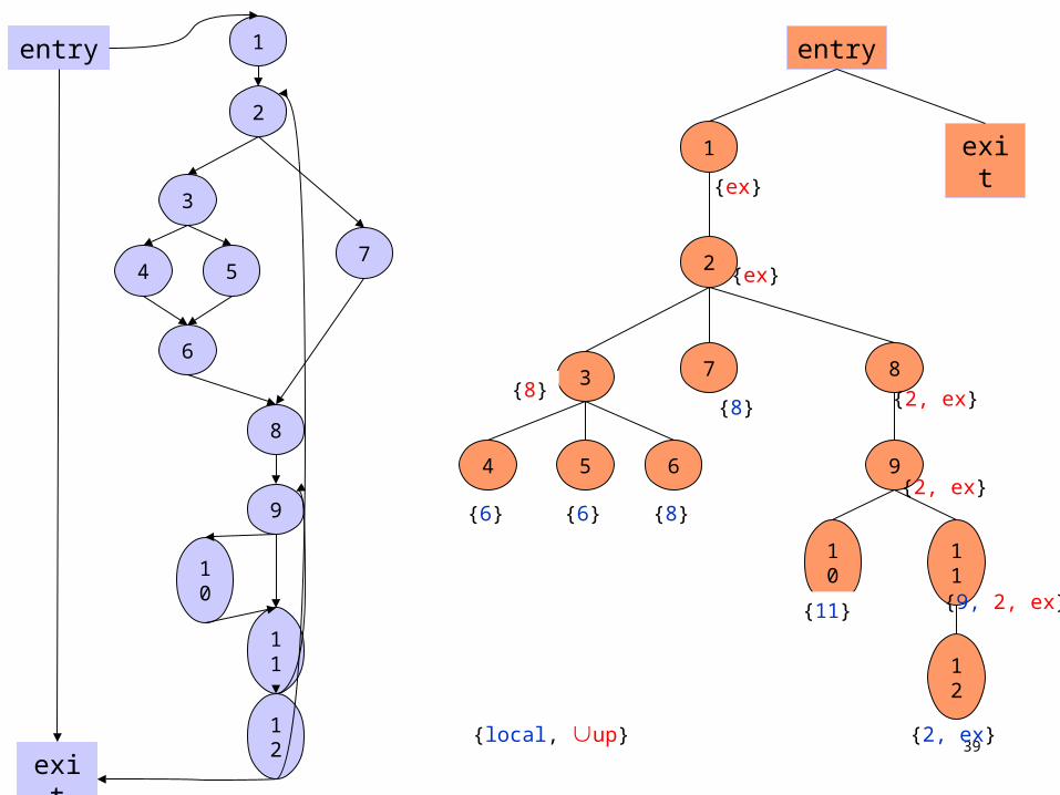
Dominance frontier

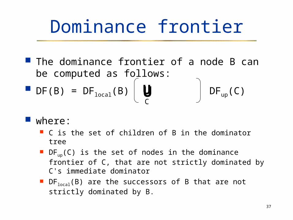
The dominance frontier of a node B can be computed as follows:

DF(B) = DFlocal(B) U DFup(C)

where: C is the set of children of B in the dominator tree DFup(C) is the set of nodes in the dominance frontier of C,

that are not strictly dominated by C's immediate dominator DFlocal(B) are the successors of B that are not strictly

dominated by B.

UC

38

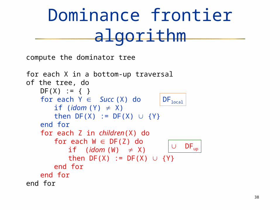
Dominance frontier algorithm

compute the dominator tree

for each X in a bottom-up traversal of the tree, do

DF(X) := { }for each Y Succ (X) do

if (idom (Y) X)then DF(X) := DF(X) {Y}

end forfor each Z in children(X) do

for each W DF(Z) doif (idom (W) X)then DF(X) := DF(X) {Y}

end forend for

end for

DFlocal

DFup

39

1

2

3

4 57

8

9

10

12

6

11

exit

entry entry

1 exit

2

3 7 8

4 5 6 9

10

11

12

{2, ex}

{9, 2, ex}{11}

{2, ex}

{2, ex}

{6} {8}

{8}{8}

{ex}

{ex}

{local, up}

{6}

40

B1

B2

B3 B4

B5

B0

B6

B7

B8 B9

B10

B11

entry

exit

entry

B0

B11 B6B1

B2

exit

B7B8

B3 B4 B5 B9

B10

{B5} {B8} {B6} {B10}

{exit}{B8, B6}{B10} {B8, B10}

{B6} {B6, exit} {exit}

{}