Embed Size (px)
Citation preview

R.K. Bhattacharjya/CE/IITG
Introduction To Genetic Algorithms
Dr. Rajib Kumar BhattacharjyaProfessor
Department of Civil Engineering
IIT Guwahati
Email: [email protected]
24 April 2015
1

R.K. Bhattacharjya/CE/IITG
References
24 April 2015
2
D. E. Goldberg, ‘Genetic Algorithm In Search, Optimization And Machine Learning’, New York: Addison – Wesley (1989)
John H. Holland ‘Genetic Algorithms’, Scientific American Journal, July 1992.
Kalyanmoy Deb, ‘An Introduction To Genetic Algorithms’, Sadhana, Vol. 24 Parts 4 And 5.

R.K. Bhattacharjya/CE/IITG
Introduction to optimization
24 April 2015
3
Global optimaLocal optima
Local optima
Local optima
Local optima
f
X

R.K. Bhattacharjya/CE/IITG
Introduction to optimization
24 April 2015
4
Multiple optimal solutions

R.K. Bhattacharjya/CE/IITG
Genetic Algorithms
24 April 2015
5
Genetic Algorithms are the heuristic search and optimization
techniques that mimic the process of natural evolution.

R.K. Bhattacharjya/CE/IITG
Principle Of Natural Selection
24 April 2015
6
“Select The Best, Discard
The Rest”
R.K. Bhattacharjya/CE/IITG
An Example….
24 April 2015
7
Giraffes have long necks
Giraffes with slightly longer necks could feed on leaves of higher branches when all lower ones had been eaten off.
They had a better chance of survival.
Favorable characteristic propagated through generations of giraffes.
Now, evolved species has long necks.

R.K. Bhattacharjya/CE/IITG
24 April 2015
8
This longer necks may have due to the effect of mutation initially. Howeveras it was favorable, this was propagated over the generations.
An Example….

R.K. Bhattacharjya/CE/IITG
Evolution of species
24 April 2015
9
Initial
population of
animals
Struggle for
existence
Survival of the
fittest
Surviving
individuals
reproduce,
propagate
favorable
characteristicsEvolved
species

R.K. Bhattacharjya/CE/IITG
24 April 2015
10
Thus genetic algorithms implement the optimization strategies by simulating evolution of species through natural selection

R.K. Bhattacharjya/CE/IITG
Simple Genetic Algorithms
24 April 2015
11
Initialize population Evaluate Solutions
YES
T = 0
T=T+1
Selection
Crossover
Mutation
NO
Is optimum Solution ?
Start
Stop

R.K. Bhattacharjya/CE/IITG
Simple Genetic Algorithm
24 April 2015
12
function sga (){Initialize population;Calculate fitness function;
While(fitness value != termination criteria){
Selection;
Crossover;
Mutation;
Calculate fitness function;}
}
R.K. Bhattacharjya/CE/IITG
GA Operators and Parameters
24 April 2015
13
Selection
Crossover
Mutation
Now we will discuss about genetic operators

R.K. Bhattacharjya/CE/IITG
Selection
24 April 2015
14
The process that determines which solutions are to be preservedand allowed to reproduce and which ones deserve to die out.
The primary objective of the selection operator is to emphasize thegood solutions and eliminate the bad solutions in a population whilekeeping the population size constant.
“Selects the best, discards the rest”

R.K. Bhattacharjya/CE/IITG
Functions of Selection operator
24 April 2015
15
Identify the good solutions in a population
Make multiple copies of the good solutions
Eliminate bad solutions from the population so that multiple copies of good solutions can be placed in the population
Now how to identify the good solutions?

R.K. Bhattacharjya/CE/IITG
Fitness function
24 April 2015
16
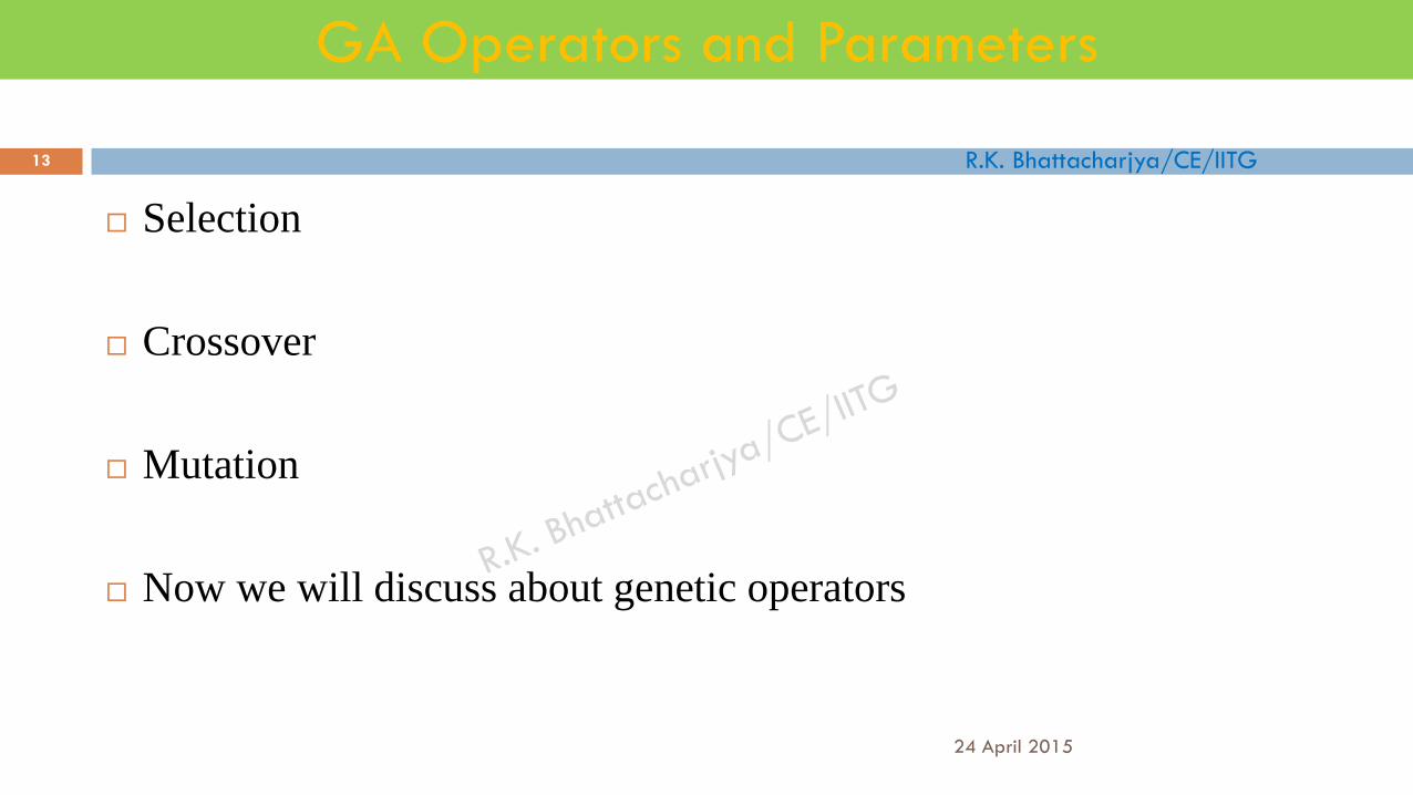
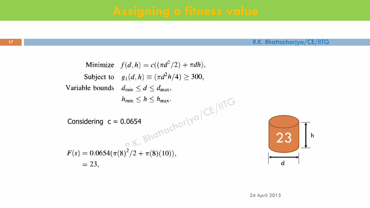
A fitness function value quantifies the optimality of a solution. The value is used to rank a particular solution against all the other solutions
A fitness value is assigned to each solution depending on how close it is actually to the optimal solution of the problem
A fitness value can be assigned to evaluate the solutions
R.K. Bhattacharjya/CE/IITG
Assigning a fitness value
24 April 2015
17
Considering c = 0.0654
23
d
h

R.K. Bhattacharjya/CE/IITG
Selection operator
24 April 2015
18
There are different techniques to implement selection in Genetic Algorithms.
They are:
Tournament selection
Roulette wheel selection
Proportionate selection
Rank selection
Steady state selection, etc

R.K. Bhattacharjya/CE/IITG
Tournament selection
24 April 2015
19
In tournament selection several tournaments are played among a few individuals. The individuals are chosen at random from the population.
The winner of each tournament is selected for next generation.
Selection pressure can be adjusted by changing the tournament size.
Weak individuals have a smaller chance to be selected if tournament size is large.

R.K. Bhattacharjya/CE/IITG
Tournament selection
24 April 2015
20
22
13 +30
22
40
32
32
25
7 +45
25
25
32
25
22
40
22
13 +30
7 +45
13 +30
22
32
25 13 +30
22
25
Selected
Best solution will have two copies
Worse solution will have no copies
Other solutions will have two, one
or zero copies
R.K. Bhattacharjya/CE/IITG
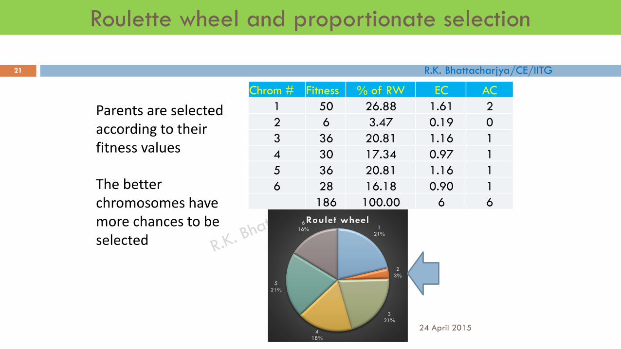
Roulette wheel and proportionate selection
24 April 2015
21
Chrom # Fitness
1 50
2 6
3 36
4 30
5 36
6 28
186
% of RW
26.88
3.47
20.81
17.34
20.81
16.18
100.00
EC
1.61
0.19
1.16
0.97
1.16
0.90
6
AC
2
0
1
1
1
1
6
121%
23%
321%
418%
521%
616%
Roulet wheel
Parents are selected according to their fitness values
The better chromosomes have more chances to be selected

R.K. Bhattacharjya/CE/IITG
Rank selection
24 April 2015
22
Chrom # Fitness
1 37
2 6
3 36
4 30
5 36
6 28
Chrom # Fitness
1 37
3 36
5 36
4 30
6 28
2 6
Sort
according
to fitness
Assign
raking
Rank
6
5
4
3
2
1
Chrom #
1
3
5
4
6
2
% of RW
29
24
19
14
10
5
Chrom #
1
3
5
4
6
2
Roulette wheel
6 5 4 3 2 1
EC AC
1.714 2
1.429 1
1.143 1
0.857 1
0.571 1
0.286 0
Chrom #
1
3
5
4
6
2

R.K. Bhattacharjya/CE/IITG
Steady state selection
24 April 2015
23
In this method, a few good chromosomes are used for creating new offspring in every iteration.
The rest of population migrates to the next generation without going through the selection process.
Then some bad chromosomes are removed and the new offspring is placed in their places
Good
Bad
New
offspringGood
New
offspring

R.K. Bhattacharjya/CE/IITG
How to implement crossover
24 April 2015
24
Source: http://www.biologycorner.com/bio1/celldivision-chromosomes.html
The crossover operator is used to create new solutions from the existing solutions available in the mating pool after applying selection operator.
This operator exchanges the gene information between the solutions in the mating pool.
0 1 0 0 1 1 0 1 1 0
Encoding of solution is necessary so that our
solutions look like a chromosome

R.K. Bhattacharjya/CE/IITG
Encoding
24 April 2015
25
The process of representing a solution in the form of a string that
conveys the necessary information.
Just as in a chromosome, each gene controls a particular characteristic of the individual, similarly, each bit in the string represents a characteristic of the solution.

R.K. Bhattacharjya/CE/IITG
Encoding Methods
24 April 2015
26
Most common method of encoding is binary coded. Chromosomes are strings of 1and 0 and each position in the chromosome represents a particular characteristic ofthe problem
Decoded value 52 26
Mapping between decimal
and binary value

R.K. Bhattacharjya/CE/IITG
Encoding Methods
24 April 2015
27
d
h (d,h) = (8,10) cm
Chromosome = [0100001010]
Defining a string [0100001010]d h

R.K. Bhattacharjya/CE/IITG
Crossover operator
24 April 2015
28
The most popular crossover selects any two solutions strings randomly from the mating pool and some portion of the strings is exchanged between the strings.
The selection point is selected randomly.
A probability of crossover is also introduced in order to give freedom to an individual solution string to determine whether the solution would go for crossover or not.Solution 1
Solution 2
Child 1
Child 2

R.K. Bhattacharjya/CE/IITG
Binary Crossover
24 April 2015
29
Source: Deb 1999

R.K. Bhattacharjya/CE/IITG
Mutation operator
24 April 2015
30
Though crossover has the main responsibility to search for the
optimal solution, mutation is also used for this purpose.
Mutation is the occasional introduction of new features in to the
solution strings of the population pool to maintain diversity in the
population.
Before mutation After mutation

R.K. Bhattacharjya/CE/IITG
Binary Mutation
24 April 2015
31
Mutation operator changes a 1 to 0 or vise versa, with a mutation probability of .
The mutation probability is generally kept low for steady convergence.
A high value of mutation probability would search here and there like a random search
technique.
Source: Deb 1999

R.K. Bhattacharjya/CE/IITG
Elitism
24 April 2015
32
Crossover and mutation may destroy the best solution of the population pool
Elitism is the preservation of few best solutions of the population pool
Elitism is defined in percentage or in number

R.K. Bhattacharjya/CE/IITG
Nature to Computer Mapping
24 April 2015
33
Nature ComputerPopulation
Individual
Fitness
Chromosome
Gene
Reproduction
Set of solutions
Solution to a problem
Quality of a solution
Encoding for a solution
Part of the encoding solution
Crossover

R.K. Bhattacharjya/CE/IITG
An example problem
24 April 2015
34
Consider 6 bit string to represent the solution, then00000 = 0 and 11111 =
Assume population size of 4
Let us solve this problem by hand calculation

R.K. Bhattacharjya/CE/IITG
24 April 2015
35
Actual
count
2
1
0
1
Sol No Binary
String
1 100101
2 001100
3 111010
4 101110
DV
37
12
58
46
x
value
0.587
0.19
0.921
0.73
f
0.96
0.56
0.25
0.75
Avg
Max
F
0.96
0.56
0.25
0.75
2.25
0.96
Relative
Fitness
0.38
0.22
0.10
0.30
Expected
count
1.53
0.89
0.39
1.19
Initialize
population
Calculate decoded
value
Calculate real
value
Calculate objective
function value
Calculate fitness
value
Calculate relative
fitness value
Calculate
expected count
Calculate actual
count
Selection: Proportionate selectionInitial populationFitness
calculationDecoding
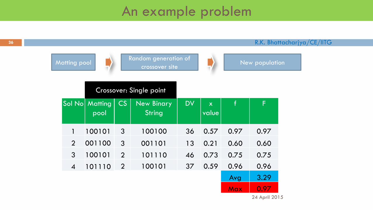
An example problem
R.K. Bhattacharjya/CE/IITG
24 April 2015
36
Sol No Matting
pool
1 100101
2 001100
3 100101
4 101110
f F
0.97 0.97
0.60 0.60
0.75 0.75
0.96 0.96
Avg 3.29
Max 0.97
CS
3
3
2
2
New Binary
String
100100
001101
101110
100101
DV
36
13
46
37
x
value
0.57
0.21
0.73
0.59
Matting poolRandom generation of
crossover siteNew population
Crossover: Single point
An example problem

R.K. Bhattacharjya/CE/IITG
24 April 2015
37
Sol No
1
2
3
4
Population
after crossover
100100
001101
101110
100101
Population
after mutation
100000
101101
100110
101101
f F
1.00 1.00
0.78 0.78
0.95 0.95
0.78 0.78
Avg 3.51
Max 1.00
DV
32
45
38
45
x
value
0.51
0.71
0.60
0.71
Mutation
An example problem

R.K. Bhattacharjya/CE/IITG
Real coded Genetic Algorithms
24 April 2015
38
Disadvantage of binary coded GA
more computation
lower accuracy
longer computing time
solution space discontinuity
hamming cliff

R.K. Bhattacharjya/CE/IITG
Real coded Genetic Algorithms
24 April 2015
39
The standard genetic algorithms has the following steps
1. Choose initial population
2. Assign a fitness function
3. Perform elitism
4. Perform selection
5. Perform crossover
6. Perform mutation
In case of standard Genetic Algorithms, steps 5 and 6 require bitwise manipulation.

R.K. Bhattacharjya/CE/IITG
Real coded Genetic Algorithms
24 April 2015
40
Simple crossover: similar to binary crossover
P1=[8 6 3 7 6]
P2=[2 9 4 8 9]
C1=[8 6 4 8 9]
C2=[2 9 3 7 6]

R.K. Bhattacharjya/CE/IITG
Real coded Genetic Algorithms
24 April 2015
41
Linear Crossover
• Parents: (x1,…,xn ) and (y1,…,yn )
• Select a single gene (k) at random
• Three children are created as,
) ..., ,5.05.0 , ..., ,( 1 nkkk xxyxx
) ..., ,5.05.1 , ..., ,( 1 nkkk xxyxx
) ..., ,5.15.0- , ..., ,( 1 nkkk xxyxx
• From the three children, best two are selected for the
next generation

R.K. Bhattacharjya/CE/IITG
Real coded Genetic Algorithms
24 April 2015
42
Single arithmetic crossover
• Parents: (x1,…,xn ) and (y1,…,yn )
• Select a single gene (k) at random
• child1 is created as,
• reverse for other child. e.g. with = 0.5
) ..., ,)1( , ..., ,( 1 nkkk xxyxx
0.1 0.3 0.1 0.3 0.7 0.2 0.5 0.1 0.2
0.5 0.7 0.7 0.5 0.2 0.8 0.3 0.9 0.4
0.1 0.3 0.1 0.3 0.7 0.5 0.5 0.1 0.2
0.5 0.7 0.7 0.5 0.2 0.5 0.3 0.9 0.4

R.K. Bhattacharjya/CE/IITG
Real coded Genetic Algorithms
24 April 2015
43
Simple arithmetic crossover
• Parents: (x1,…,xn ) and (y1,…,yn )
• Pick random gene (k) after this point mix values
• child1 is created as:
• reverse for other child. e.g. with = 0.5
))1(n
y ..., ,1
)1(1
, ..., ,1
(n
xk
xk
yk
xx
0.1 0.3 0.1 0.3 0.7 0.2 0.5 0.1 0.2
0.5 0.7 0.7 0.5 0.2 0.8 0.3 0.9 0.4
0.1 0.3 0.1 0.3 0.7 0.5 0.4 0.5 0.3
0.5 0.7 0.7 0.5 0.2 0.5 0.4 0.5 0.3

R.K. Bhattacharjya/CE/IITG
Real coded Genetic Algorithms
24 April 2015
44
Whole arithmetic crossover
• Most commonly used
• Parents: (x1,…,xn ) and (y1,…,yn )
• child1 is:
• reverse for other child. e.g. with = 0.5
yx )1(
0.1 0.3 0.1 0.3 0.6 0.2 0.5 0.1 0.2
0.5 0.7 0.7 0.5 0.2 0.8 0.3 0.9 0.4
0.3 0.5 0.4 0.4 0.4 0.5 0.4 0.5 0.3
0.3 0.5 0.4 0.4 0.4 0.5 0.4 0.5 0.3

R.K. Bhattacharjya/CE/IITG
Simulated binary crossover
24 April 2015
45
Developed by Deb and Agrawal, 1995)
Where, a random number
is a parameter that controls the crossover process. A high value of the parameter will create near-parent solution

R.K. Bhattacharjya/CE/IITG
Random mutation
24 April 2015
46
Where is a random number between [0,1]
Where, is the user defined maximum perturbation

R.K. Bhattacharjya/CE/IITG
Normally distributed mutation
24 April 2015
47
A simple and popular method
Where is the Gaussian probability distribution with zero
mean

R.K. Bhattacharjya/CE/IITG
Polynomial mutation
24 April 2015
48

R.K. Bhattacharjya/CE/IITG
Multi-modal optimization
24 April 2015
49

R.K. Bhattacharjya/CE/IITG
After Generation 200
24 April 2015
50

R.K. Bhattacharjya/CE/IITG
Multi-modal optimization
24 April 2015
51
Niche count
Modified fitness
Sharing function

R.K. Bhattacharjya/CE/IITG
Hand calculation
24 April 2015
52
Maximize
Sol String Decoded
value
x f
1 110100 52 1.651 0.890
2 101100 44 1.397 0.942
3 011101 29 0.921 0.246
4 001011 11 0.349 0.890
5 110000 48 1.524 0.997
6 101110 46 1.460 0.992

R.K. Bhattacharjya/CE/IITG
Distance table
24 April 2015
53
dij 1 2 3 4 5 6
1 0 0.254 0.73 1.302 0.127 0.191
2 0.254 0 0.476 1.048 0.127 0.063
3 0.73 0.476 0 0.572 0.603 0.539
4 1.302 1.048 0.572 0 1.175 1.111
5 0.127 0.127 0.603 1.175 0 0.064
6 0.191 0.063 0.539 1.111 0.064 0
R.K. Bhattacharjya/CE/IITG
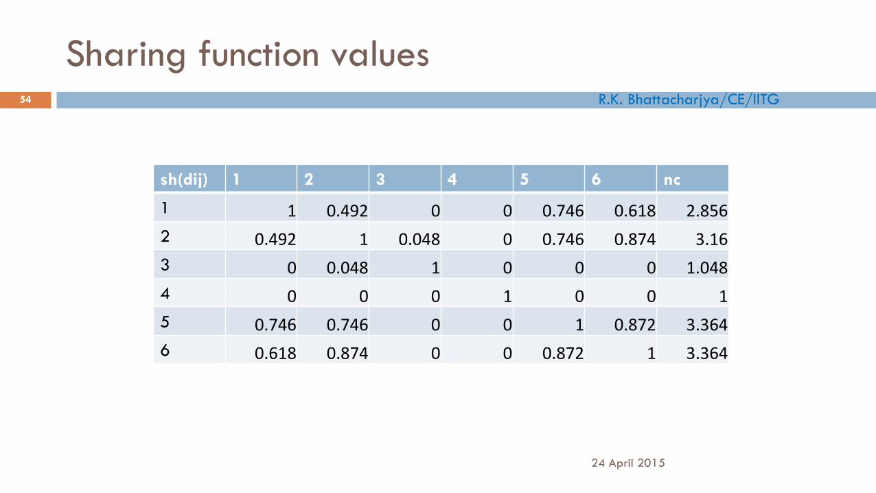
Sharing function values
24 April 2015
54
sh(dij) 1 2 3 4 5 6 nc
1 1 0.492 0 0 0.746 0.618 2.856
2 0.492 1 0.048 0 0.746 0.874 3.16
3 0 0.048 1 0 0 0 1.048
4 0 0 0 1 0 0 1
5 0.746 0.746 0 0 1 0.872 3.364
6 0.618 0.874 0 0 0.872 1 3.364

R.K. Bhattacharjya/CE/IITG
Sharing fitness value
24 April 2015
55
Sol String Decoded
value
x f nc f’
1 110100 52 1.651 0.890 2.856 0.312
2 101100 44 1.397 0.942 3.160 0.300
3 011101 29 0.921 0.246 1.048 0.235
4 001011 11 0.349 0.890 1.000 0.890
5 110000 48 1.524 0.997 3.364 0.296
6 101110 46 1.460 0.992 3.364 0.295

R.K. Bhattacharjya/CE/IITG
Solutions obtained using modified fitness value
24 April 2015
56
R.K. Bhattacharjya/CE/IITG
Evolutionary Strategies
24 April 2015
57
ES use real parameter value
ES does not use crossover operator
It is just like a real coded genetic algorithms with selection and
mutation operators only

R.K. Bhattacharjya/CE/IITG
Two members ES: (1+1) ES
24 April 2015
58
In each iteration one parent is used to create one offspring by using Gaussian mutation operator

R.K. Bhattacharjya/CE/IITG
Two members ES: (1+1) ES
24 April 2015
59
Step1: Choose a initial solution and a mutation strength
Step2: Create a mutate solution
Step 3: If , replace with
Step4: If termination criteria is satisfied, stop, else go to step 2

R.K. Bhattacharjya/CE/IITG
Two members ES: (1+1) ES
24 April 2015
60
Strength of the algorithm is the proper value of
Rechenberg postulate
The ratio of successful mutations to all the mutations should be 1/5. If this
ratio is greater than 1/5, increase mutation strength. If it is less than 1/5,
decrease the mutation strength.

R.K. Bhattacharjya/CE/IITG
Two members ES: (1+1) ES
24 April 2015
61
A mutation is defined as successful if the mutated offspring is better
than the parent solution.
If is the ratio of successful mutation over n trial, Schwefel (1981)
suggested a factor in the following update rule

R.K. Bhattacharjya/CE/IITG
Matlab code
24 April 2015
62

24 April 2015
63

R.K. Bhattacharjya/CE/IITG
Some results of 1+1 ES
24 April 2015
64
Optimal Solution is
X*= [3.00 1.99]
Objective function value f
= 0.0031007
1
2
2
55
10
10
10
2020
20
20
20
50
50
50
50
50
10
0
100
100100
100
100
20
020
0
200
200200
X
Y
0 0.5 1 1.5 2 2.5 3 3.5 4 4.5 50
0.5
1
1.5
2
2.5
3
3.5
4
4.5
5
R.K. Bhattacharjya/CE/IITG
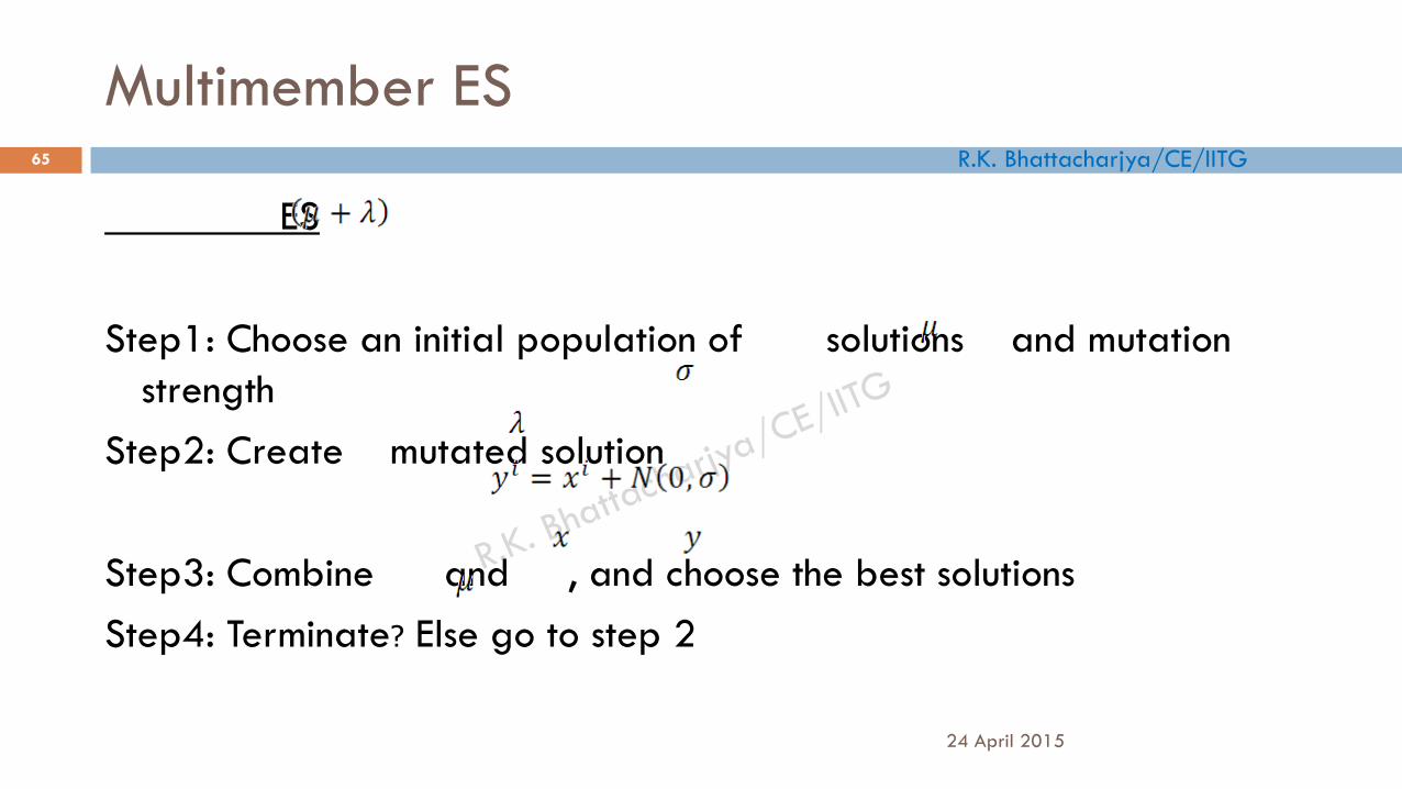
Multimember ES
24 April 2015
65
ES
Step1: Choose an initial population of solutions and mutation
strength
Step2: Create mutated solution
Step3: Combine and , and choose the best solutions
Step4: Terminate? Else go to step 2

R.K. Bhattacharjya/CE/IITG
Multimember ES
24 April 2015
66
ES
Through mutation
Through selection

R.K. Bhattacharjya/CE/IITG
Multimember ES
24 April 2015
67
ES
Off
spri
ng
Through mutation
Through selection

R.K. Bhattacharjya/CE/IITG
Multi-objective optimization
24 April 2015
68
Price
Com
fort

R.K. Bhattacharjya/CE/IITG
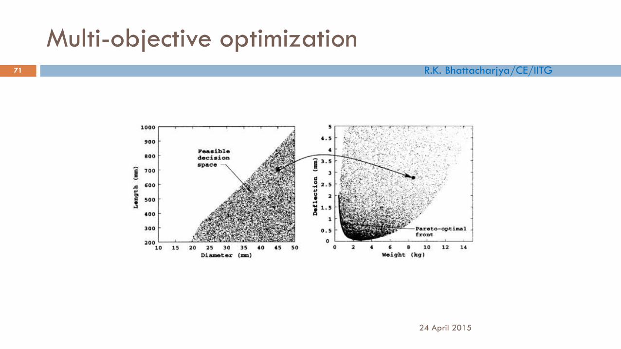
Multi-objective optimization
24 April 2015
69
Two objectives are
• Minimize weight
• Minimize deflection

R.K. Bhattacharjya/CE/IITG
Multi-objective optimization
24 April 2015
70
More than one objectives
Objectives are conflicting in nature
Dealing with two search space
Decision variable space
Objective space
Unique mapping between the objectives and often the mapping is non-linear
Properties of the two search space are not similar
Proximity of two solutions in one search space does not mean a proximity in other search space
R.K. Bhattacharjya/CE/IITG
Multi-objective optimization
24 April 2015
71
R.K. Bhattacharjya/CE/IITG
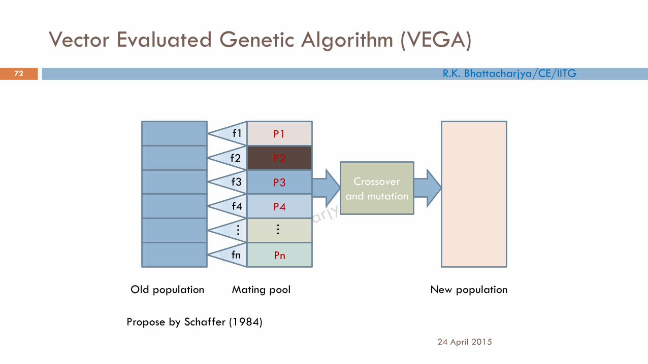
Vector Evaluated Genetic Algorithm (VEGA)
24 April 2015
72
f1
f2
f3
f4
…
fn
P1
P2
P3
P4
Pn
…
Crossover
and mutation
Old population Mating pool New population
Propose by Schaffer (1984)

R.K. Bhattacharjya/CE/IITG
Non-dominated selection heuristic
24 April 2015
73
Give more emphasize on the non-dominated solutions in the population
This can be implemented by subtracting € from the dominated solution
fitness value
Suppose N' is the number of sub-population and n' is the non-
dominated solution. Then total reduction is (N' - n')€.
The total reduction is then redistributed among the non-dominated
solution by adding an amount (N' - n')€ /n.

R.K. Bhattacharjya/CE/IITG
Non-dominated selection heuristic
24 April 2015
74
This method has two main implications
Non-dominated solutions are given more importance
Additional equal emphasis has been given to all the non-
dominated solution
R.K. Bhattacharjya/CE/IITG
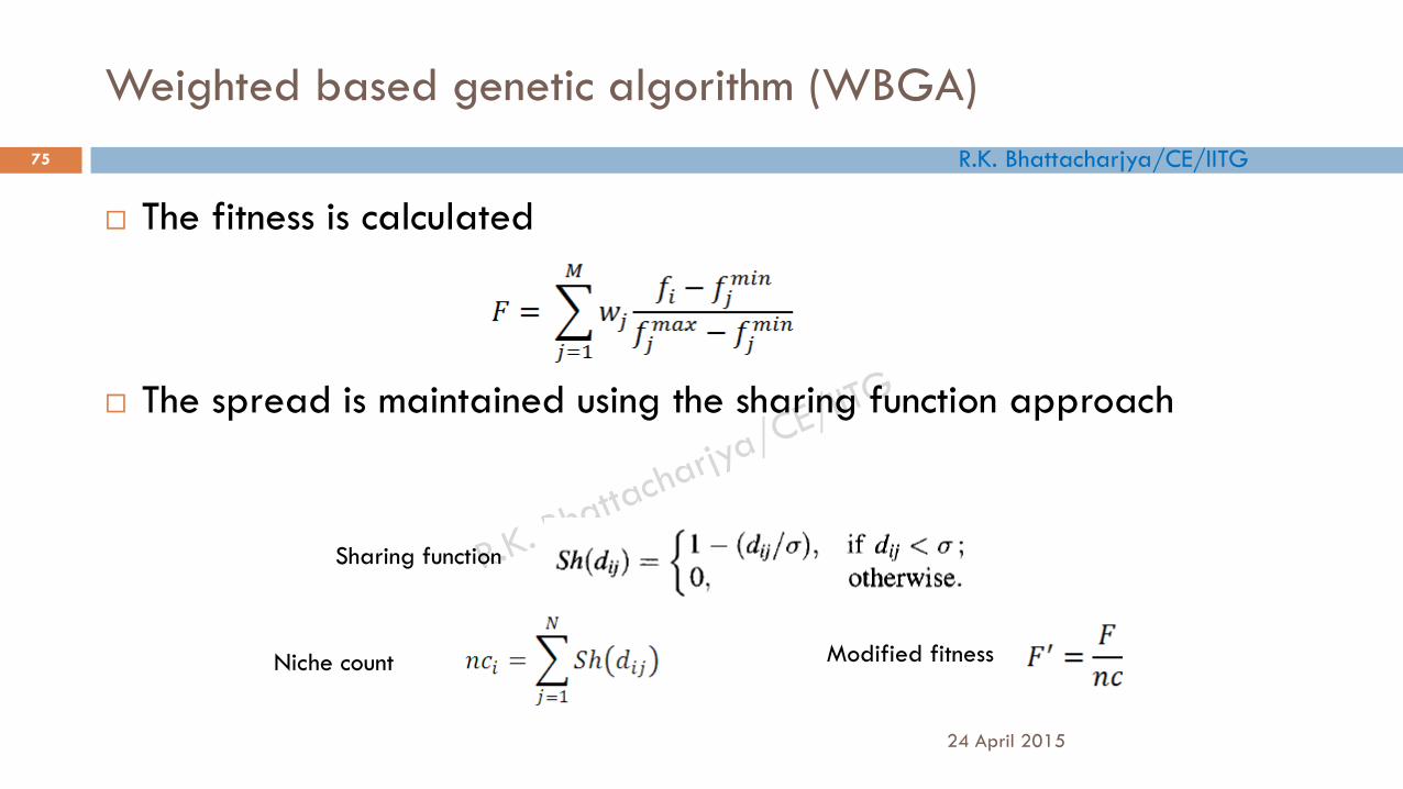
Weighted based genetic algorithm (WBGA)
24 April 2015
75
The fitness is calculated
The spread is maintained using the sharing function approach
Niche count Modified fitness
Sharing function

R.K. Bhattacharjya/CE/IITG
Multiple objective genetic algorithm (MOGA)
24 April 2015
76
0.1 0.2 0.3 0.4 0.5 0.6 0.7 0.8 0.9 10
0.5
1
1.5
2
2.5
3
3.5
4
4.5
5
x1
x2
0.1 0.2 0.3 0.4 0.5 0.6 0.7 0.8 0.9 10
10
20
30
40
50
60
f1
f2
Solution space Objective space

R.K. Bhattacharjya/CE/IITG
Minimize f1
Min
imiz
e f
2
Multiple objective genetic algorithm (MOGA)

R.K. Bhattacharjya/CE/IITG
Multiple objective genetic algorithm (MOGA)
24 April 2015
78
Fonseca and Fleming (1993) first introduced multiple objective genetic
algorithm (MOGA)
The assigned fitness value based on the non-dominated ranking.
The rank is assigned as where is the ranking of the ith
solution and is the number of solutions that dominate the solution.

1
1
1
1
2
2
3
Multiple objective genetic algorithm (MOGA)

R.K. Bhattacharjya/CE/IITG
24 April 2015
80
Fonseca and Fleming (1993) maintain the diversity among the non-
dominated solution using niching among the solution of same rank.
The normalize distance was calculated as,
The niche count was calculated as,
Multiple objective genetic algorithm (MOGA)

R.K. Bhattacharjya/CE/IITG
NSGA
24 April 2015
81
Srinivas and Deb (1994) proposed NSGA
The algorithm is based on the non-dominated sorting.
The spread on the Pareto optimal front is maintained using sharing
function

R.K. Bhattacharjya/CE/IITG
NSGA II
24 April 2015
82
Non-dominated Sorting Genetic Algorithms
NSGA II is an elitist non-dominated sorting Genetic Algorithm to solve multi-
objective optimization problem developed by Prof. K. Deb and his student
at IIT Kanpur.
It has been reported that NSGA II can converge to the global Pareto-
optimal front and can maintain the diversity of population on the Pareto-
optimal front

R.K. Bhattacharjya/CE/IITG
Non-dominated sorting
24 April 2015
83
Objective 1 (Minimize)
Ob
ject
ive
2 (
Min
imiz
e)
1
2
3
4
5
6
Objective 1 (Minimize)
Ob
ject
ive
2 (
Min
imiz
e)
1
2 3
4
5 Infeasible Region
Feasible Region
R.K. Bhattacharjya/CE/IITG
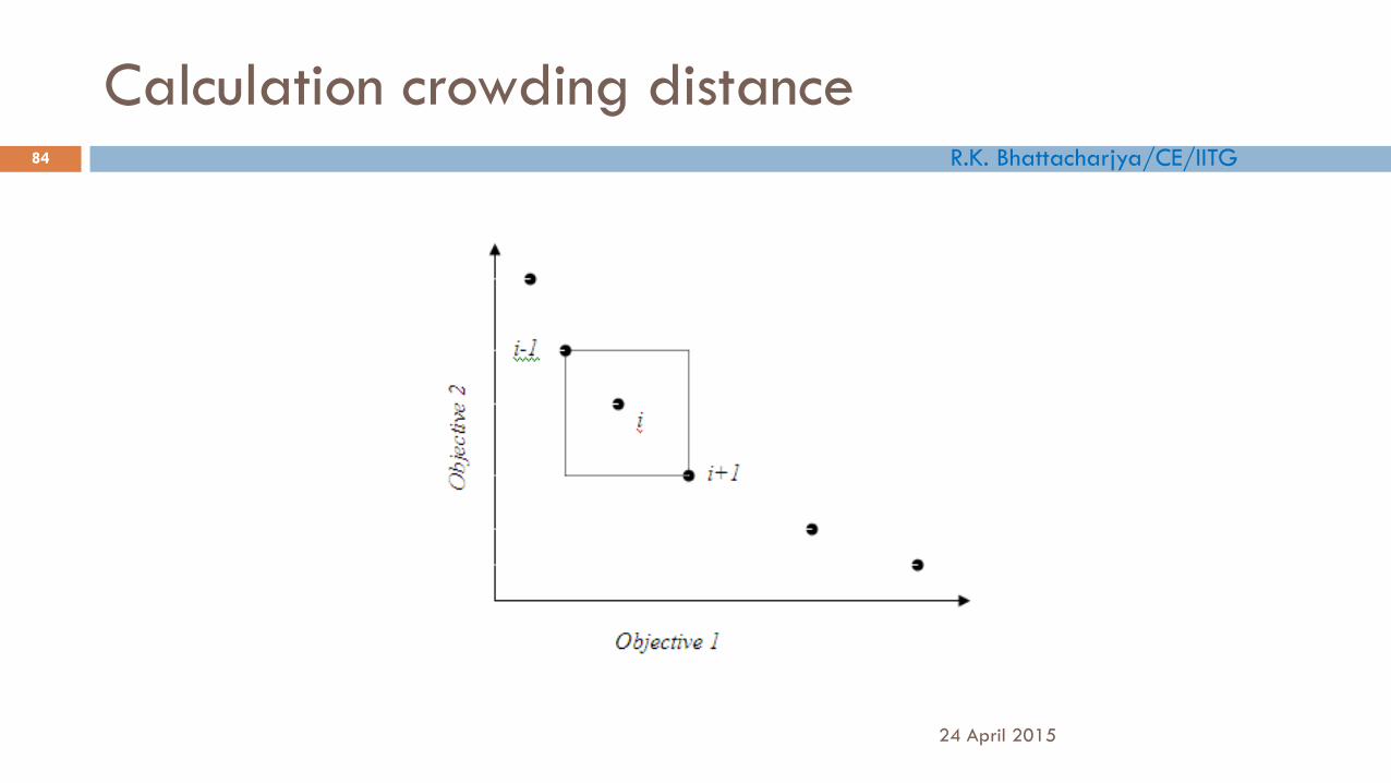
Calculation crowding distance
24 April 2015
84

R.K. Bhattacharjya/CE/IITG
Crowded tournament operator
24 April 2015
85
A solution I wins a tournament with another solution j,
If the solution i has better rank than j, i.e. ri<rj
If they have the sa,e rank, but i has a better crowding distance than j, i.e.
ri=rj and di>dj.

R.K. Bhattacharjya/CE/IITG
Replacement scheme of NSGA II
24 April 2015
86
Pt+1
Pt
Qt
F1
F2
F3
Non-dominating sorting
Crowding distance
sorting
Rejected

Initialize population of size N
Calculate all the objective functions
Rank the population according to non-
dominating criteria
Selection
Crossover
Mutation
Calculate objective function of the
new population
Combine old and new population
Non-dominating ranking on the
combined population
Replace parent population by the better
members of the combined population
Calculate crowding distance of all
the solutions
Get the N member from the
combined population on the basis
of rank and crowding distance
Termination
Criteria?
Pareto-optimal solution
Yes
No
24 April 2015
87

R.K. Bhattacharjya/CE/IITG
THANKS
24 April 2015
88