1

Lecture Ten

2

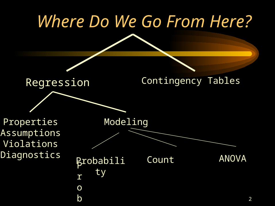
Where Do We Go From Here?

Regression

PropertiesAssumptions

ViolationsDiagnostics

Modeling

Probability

Probability Count ANOVA

Contingency Tables

3

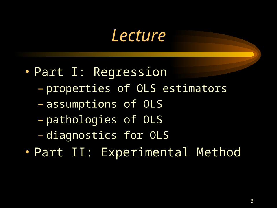
Lecture

• Part I: Regression– properties of OLS estimators– assumptions of OLS– pathologies of OLS– diagnostics for OLS

• Part II: Experimental Method

4

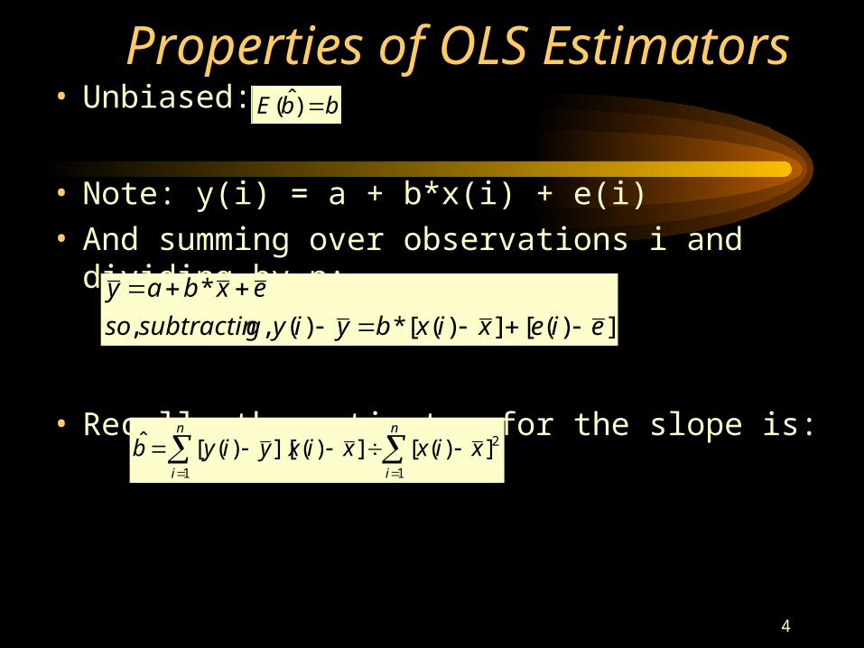
Properties of OLS Estimators• Unbiased:

• Note: y(i) = a + b*x(i) + e(i)• And summing over observations i and dividing by n:

• Recall, the estimator for the slope is:

bbE )ˆ(

])([])([*)(,,

*

eiexixbyiygsubtractinso

exbay

n

i

n

i

xixxixyiyb1 1

2])([])(][)([ˆ

5

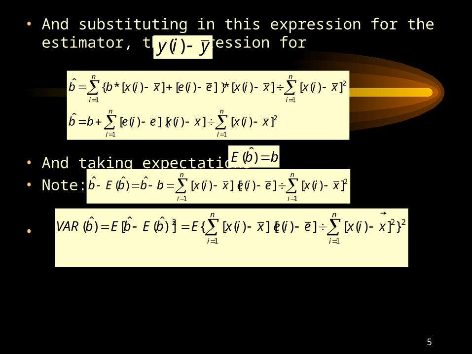
• And substituting in this expression for the estimator, the expression for

• And taking expectations

• Note:

•

yiy )(

n

i

n

i

n

i

n

i

xixxixeiebb

xixxixeiexixbb

1 1

2

1

2

1

])([])(][)([ˆ

])([])([*]})([])([*{ˆ

bbE )ˆ(

n

i

n

i

xixeiexixbbbEb1 1

2])([])(][)([ˆ)ˆ(ˆ

n

i

n

i

xixeiexixEbEbEbVAR1 1

222 }])([])(][)([{)]ˆ(ˆ[)ˆ(

6

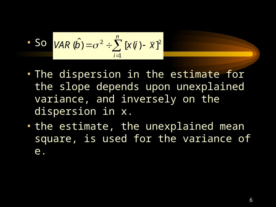
• So

• The dispersion in the estimate for the slope depends upon unexplained variance, and inversely on the dispersion in x.

• the estimate, the unexplained mean square, is used for the variance of e.

n

i

xixbVAR1

22 ])([)ˆ(

7

Other Properties of Estimators

• Efficiency: makes optimum use of the sample information to obtain estimators with minimum dispersion

• Consistency: As the sample size increases the estimator approaches the population parameter

8

Outline: Regression

• The Assumptions of Least Squares

• The Pathologies of Least Squares

• Diagnostics for Least Squares

Assumptions

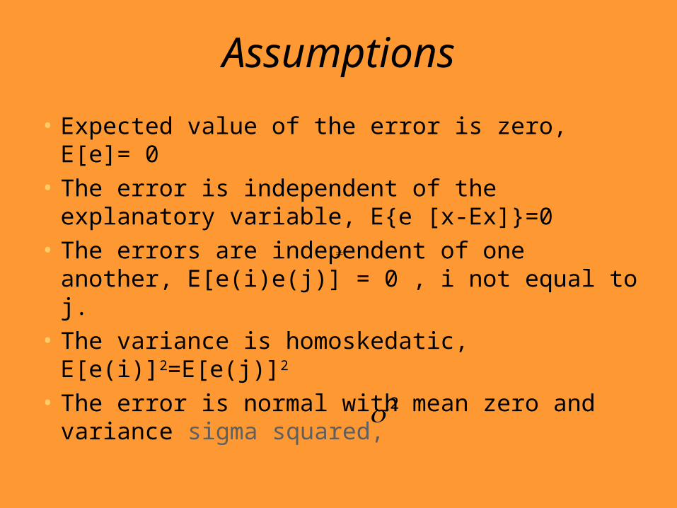
• Expected value of the error is zero, E[e]= 0

• The error is independent of the explanatory variable, E{e [x-Ex]}=0

• The errors are independent of one another, E[e(i)e(j)] = 0 , i not equal to j.

• The variance is homoskedatic, E[e(i)]2=E[e(j)]2

• The error is normal with mean zero and variance sigma squared,

2

10

18.4 Error Variable: Required Conditions

• The error is a critical part of the regression model.• Four requirements involving the distribution of

must be satisfied.– The probability distribution of is normal.– The mean of is zero: E() = 0.

– The standard deviation of is for all values of x.

– The set of errors associated with different values of y are all independent.

The Normality of

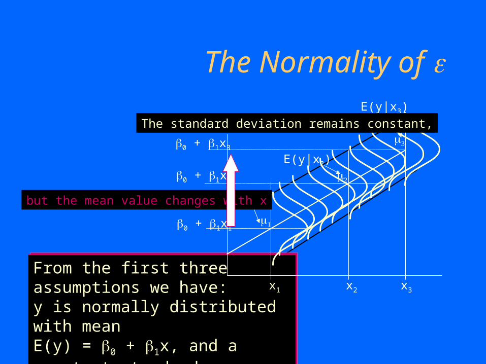
From the first three assumptions we have:y is normally distributed with meanE(y) = 0 + 1x, and a constant standard deviation

From the first three assumptions we have:y is normally distributed with meanE(y) = 0 + 1x, and a constant standard deviation

0 + 1x1

0 + 1x2

0 + 1x3

E(y|x2)

E(y|x3)

x1 x2 x3

E(y|x1)

The standard deviation remains constant,

but the mean value changes with x

12

Pathologies

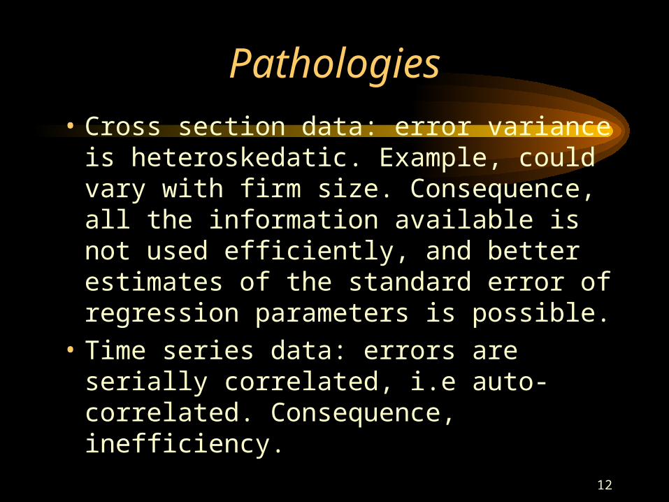
• Cross section data: error variance is heteroskedatic. Example, could vary with firm size. Consequence, all the information available is not used efficiently, and better estimates of the standard error of regression parameters is possible.

• Time series data: errors are serially correlated, i.e auto-correlated. Consequence, inefficiency.

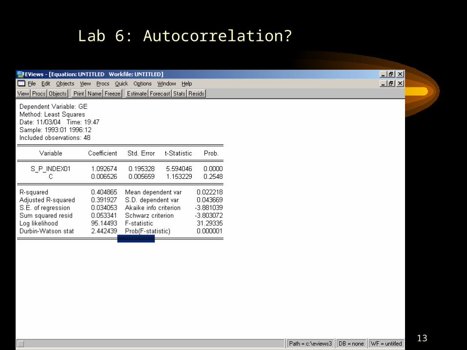
13

Lab 6: Autocorrelation?

14

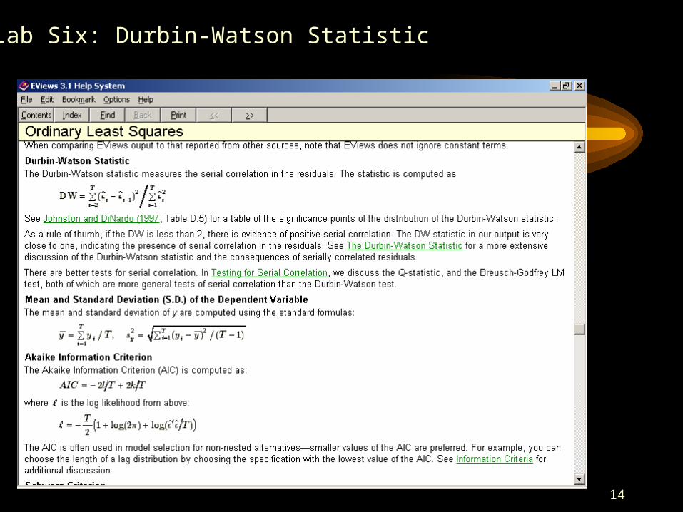
Lab Six: Durbin-Watson Statistic

15

16

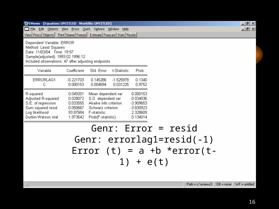
Genr: Error = residGenr: errorlag1=resid(-1)

Error (t) = a +b *error(t-1) + e(t)

17

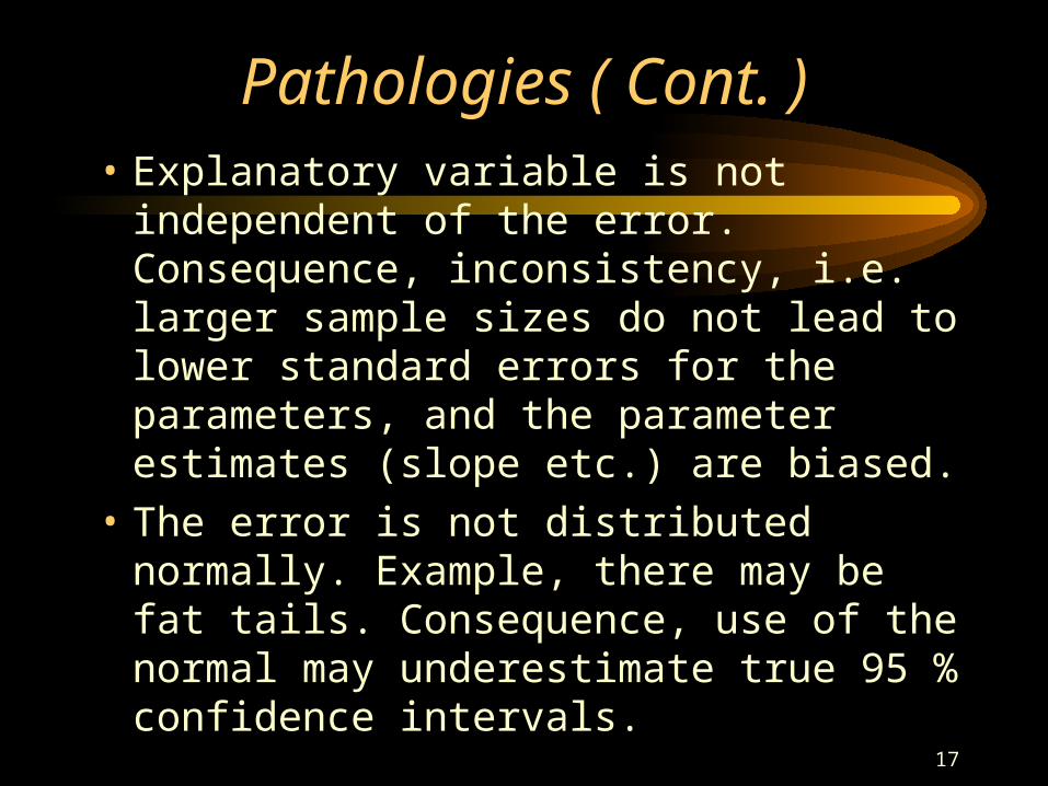
Pathologies ( Cont. )• Explanatory variable is not independent of

the error. Consequence, inconsistency, i.e. larger sample sizes do not lead to lower standard errors for the parameters, and the parameter estimates (slope etc.) are biased.

• The error is not distributed normally. Example, there may be fat tails. Consequence, use of the normal may underestimate true 95 % confidence intervals.

18

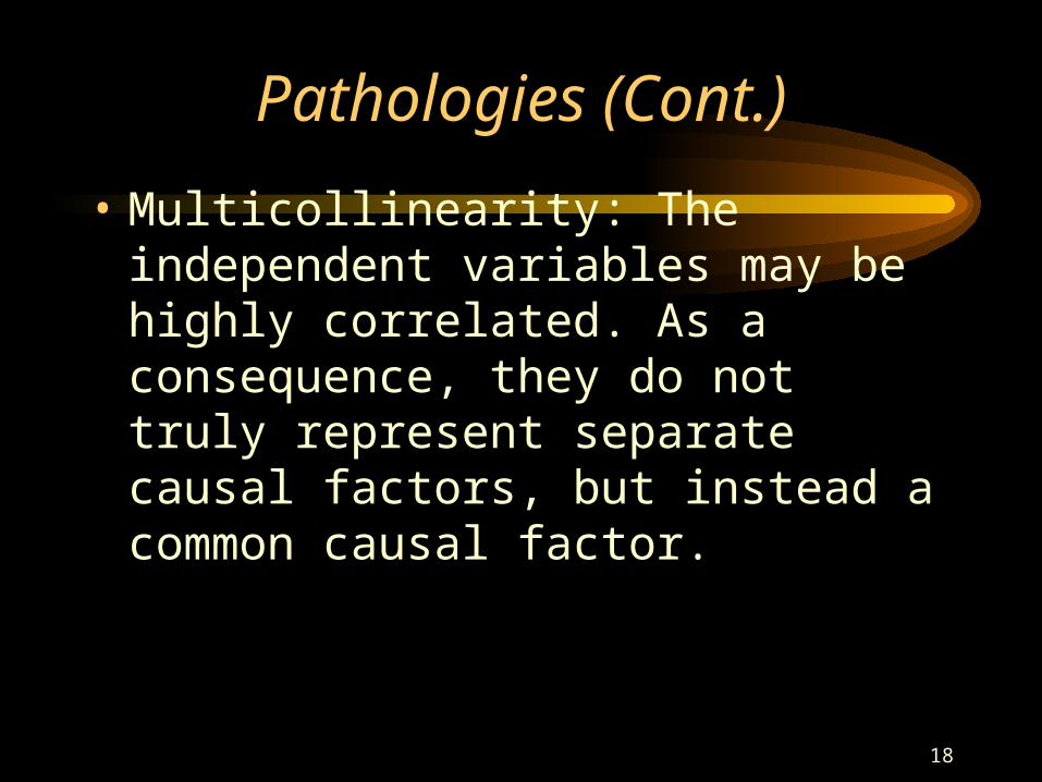
Pathologies (Cont.)

• Multicollinearity: The independent variables may be highly correlated. As a consequence, they do not truly represent separate causal factors, but instead a common causal factor.

19

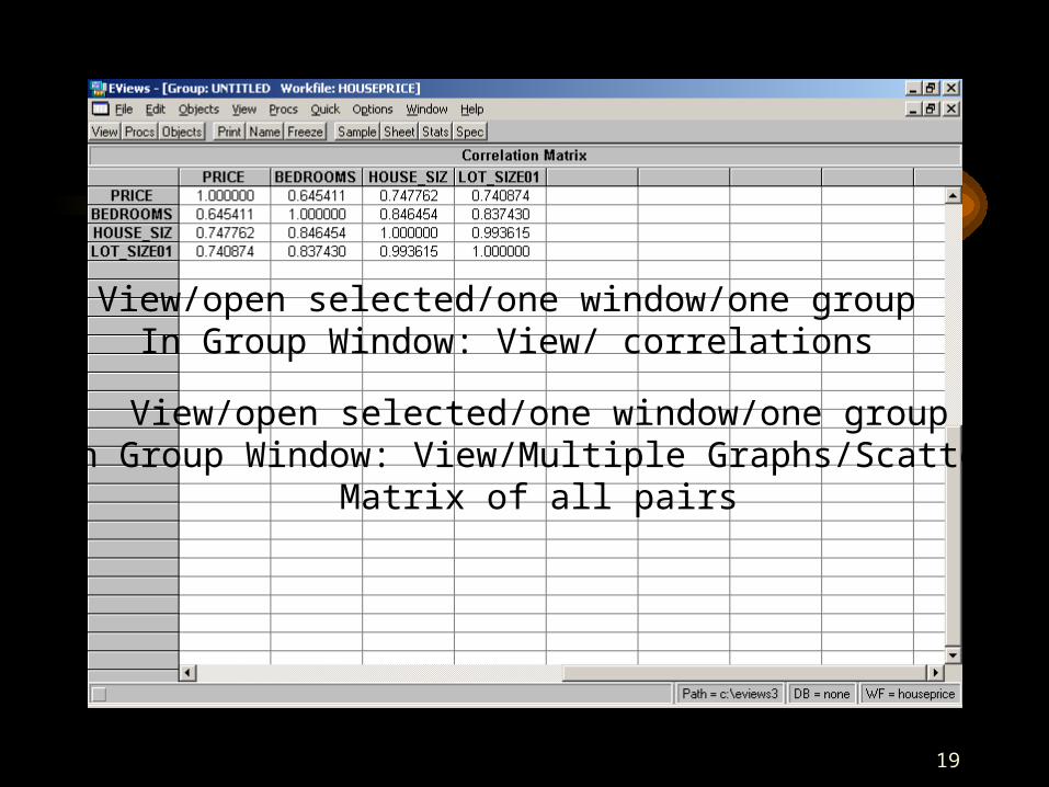
View/open selected/one window/one groupIn Group Window: View/ correlations

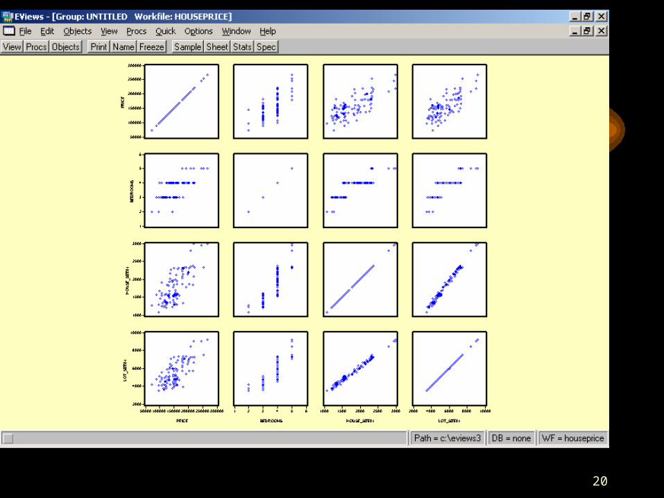
View/open selected/one window/one groupIn Group Window: View/Multiple Graphs/Scatter/

Matrix of all pairs

20

21

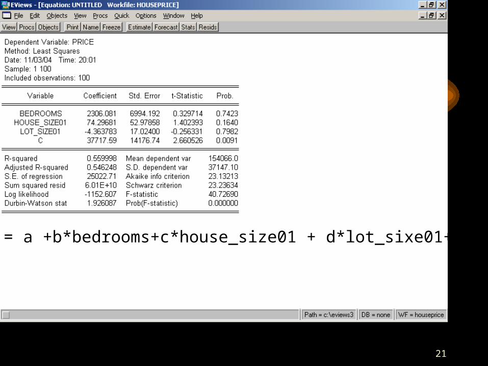
Price = a +b*bedrooms+c*house_size01 + d*lot_sixe01+e

22

23

24

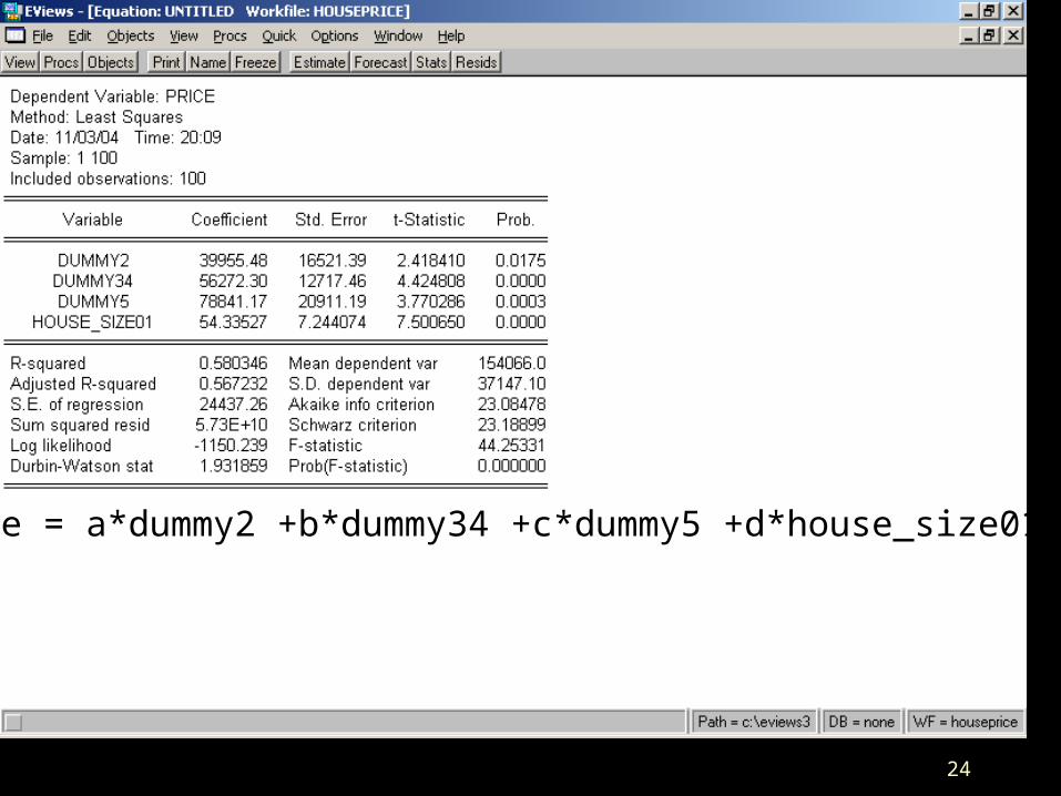
Price = a*dummy2 +b*dummy34 +c*dummy5 +d*house_size01 +e

25

18.9 Regression Diagnostics - I

• The three conditions required for the validity of the regression analysis are:– the error variable is normally distributed.– the error variance is constant for all values of x.– The errors are independent of each other.

• How can we diagnose violations of these conditions?

26

Residual Analysis• Examining the residuals (or standardized

residuals), help detect violations of the required conditions.

• Example 18.2 – continued:– Nonnormality.

• Use Excel to obtain the standardized residual histogram.

• Examine the histogram and look for a bell shaped. diagram with a mean close to zero.

27

Diagnostics ( Cont. )

• Multicollinearity may be suspected if the t-statistics for the coefficients of the explanatory variables are not significant but the coefficient of determination is high. The correlation between the explanatory variable can then be calculated. To see if it is high.

28

Diagnostics

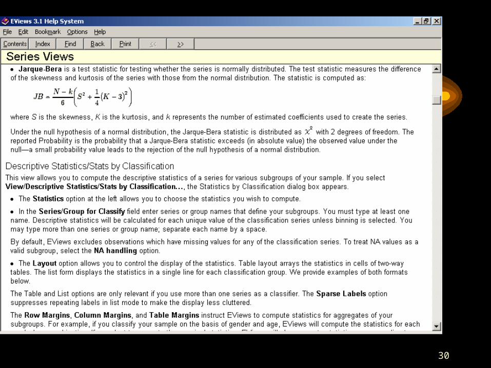
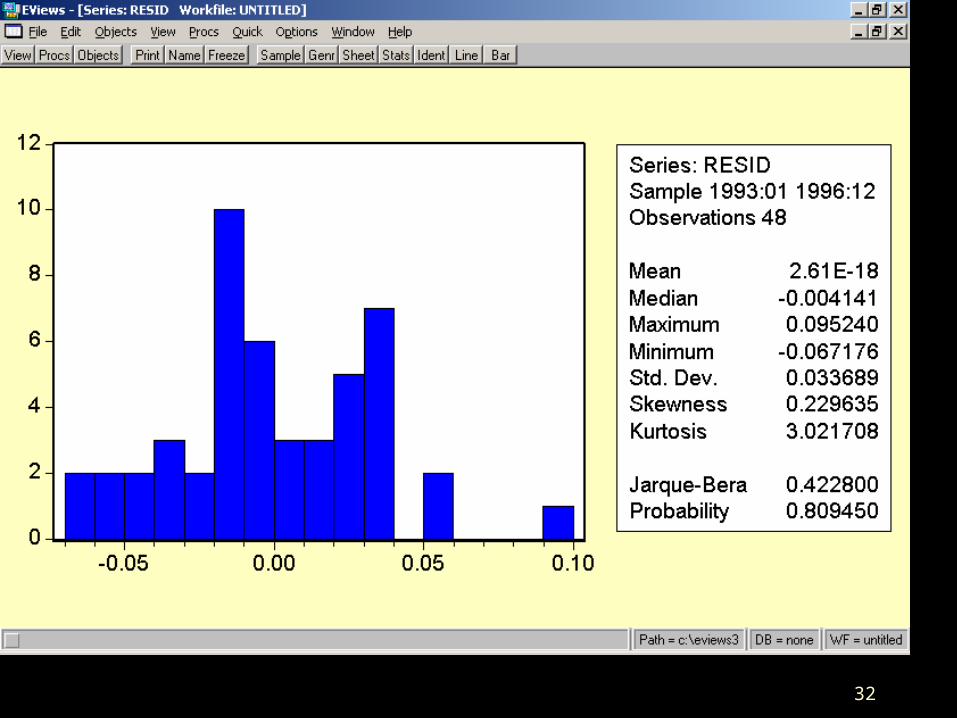
• Is the error normal? Using EViews, with the view menu in the regression window, a histogram of the distribution of the estimated error is available, along with the coefficients of skewness and kurtosis, and the Jarque-Bera statistic testing for normality.

29

Lab 6

30

31

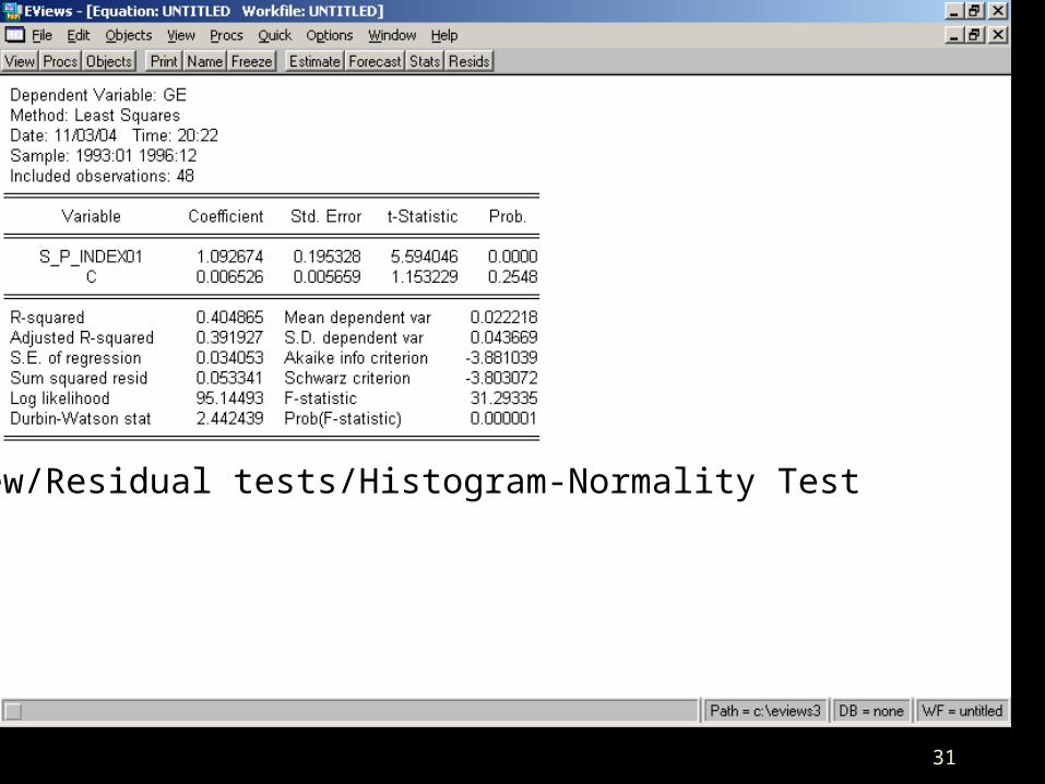
View/Residual tests/Histogram-Normality Test

32

33

Diagnostics (Cont.)

• To detect heteroskedasticity: if there are sufficient observations, plot the estimated errors against the fitted dependent variable

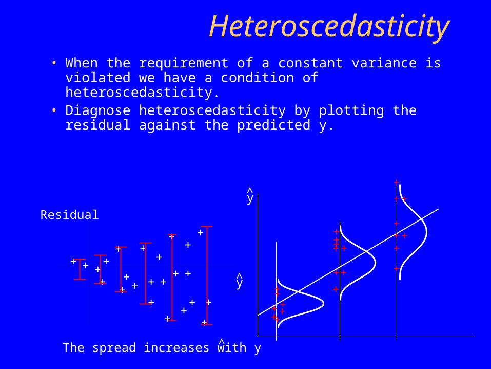
Heteroscedasticity• When the requirement of a constant variance is violated

we have a condition of heteroscedasticity.• Diagnose heteroscedasticity by plotting the residual

against the predicted y.

+ + ++

+ ++

++

+

+

+

+

+

+

+

+

+

+

++

+

+

+

The spread increases with y

y

Residualy

+

+++

+

++

+

++

+

+++

+

+

+

+

+

++

+

+

35

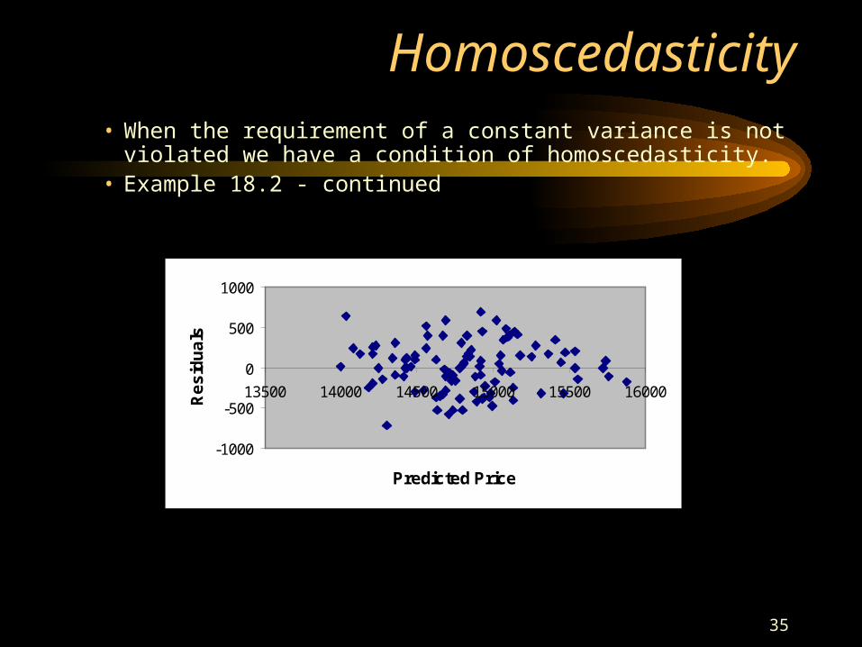
Homoscedasticity• When the requirement of a constant variance is not violated we have

a condition of homoscedasticity.• Example 18.2 - continued

-1000

-500

0

500

1000

13500 14000 14500 15000 15500 16000

Predicted Price

Re

sid

ua

ls

36

Diagnostics ( Cont.)

• Autocorrelation: The Durbin-Watson statistic is a scalar index of autocorrelation, with values near 2 indicating no autocorrelation and values near zero indicating autocorrelation. Examine the plot of the residuals in the view menu of the regression window in EViews.

37

Non Independence of Error Variables

– A time series is constituted if data were collected over time.

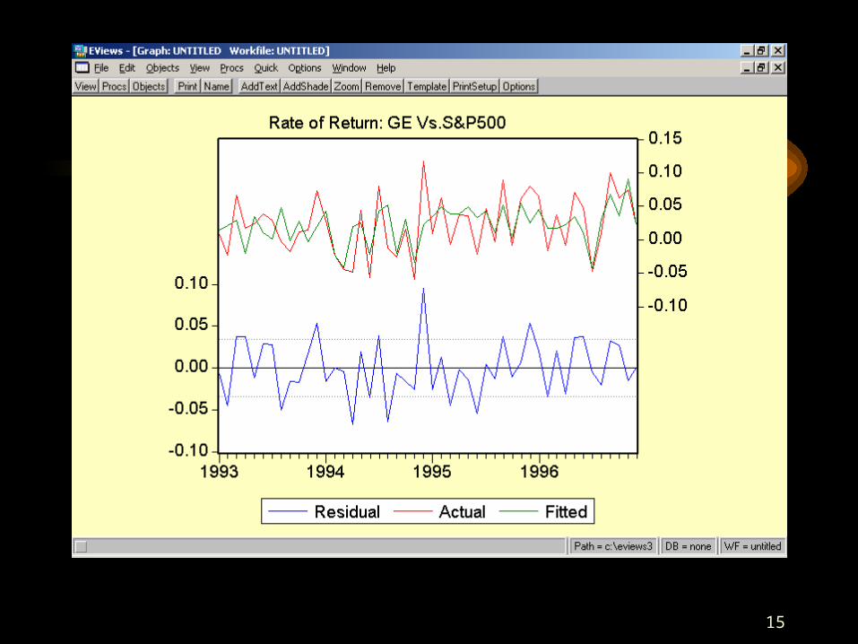
– Examining the residuals over time, no pattern should be observed if the errors are independent.

– When a pattern is detected, the errors are said to be autocorrelated.

– Autocorrelation can be detected by graphing the residuals against time.

38

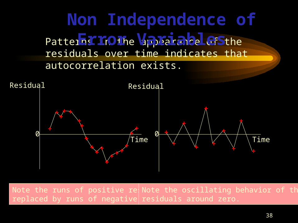
Patterns in the appearance of the residuals over time indicates that autocorrelation exists.

+

+++ +

++

++

+ +

++ + +

+

++ +

+

+

+

+

+

+Time

Residual Residual

Time+

+

+

Note the runs of positive residuals,replaced by runs of negative residuals

Note the oscillating behavior of the residuals around zero.

0 0

Non Independence of Error Variables

39

Fix-Ups

• Error is not distributed normally. For example, regression of personal income on explanatory variables. Sometimes a transformation, such as regressing the natural logarithm of income on the explanatory variables may make the error closer to normal.

40

Fix-ups (Cont.)• If the explanatory variable is not

independent of the error, look for a substitute that is highly correlated with the dependent variable but is independent of the error. Such a variable is called an instrument.

41

Data Errors: May lead to outliers

• Typos may lead to outliers and looking for ouliers is a good way to check for serious typos

42

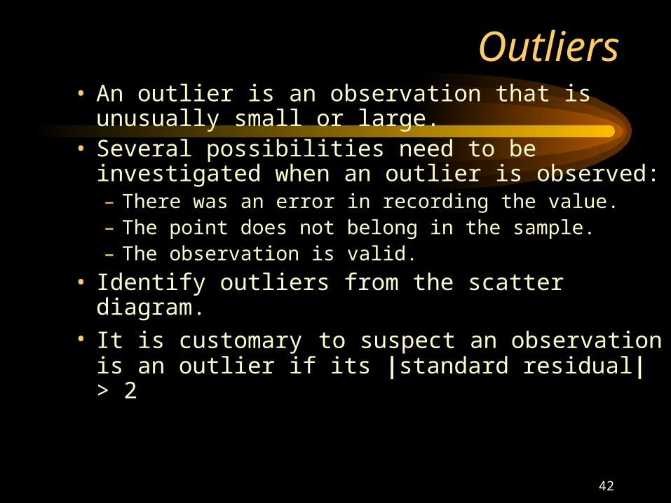
Outliers• An outlier is an observation that is unusually small or

large.• Several possibilities need to be investigated when an

outlier is observed:– There was an error in recording the value.– The point does not belong in the sample.– The observation is valid.

• Identify outliers from the scatter diagram.• It is customary to suspect an observation is an outlier

if its |standard residual| > 2

43

+

+

+

+

+ +

+ + ++

+

+

+

+

+

+

+

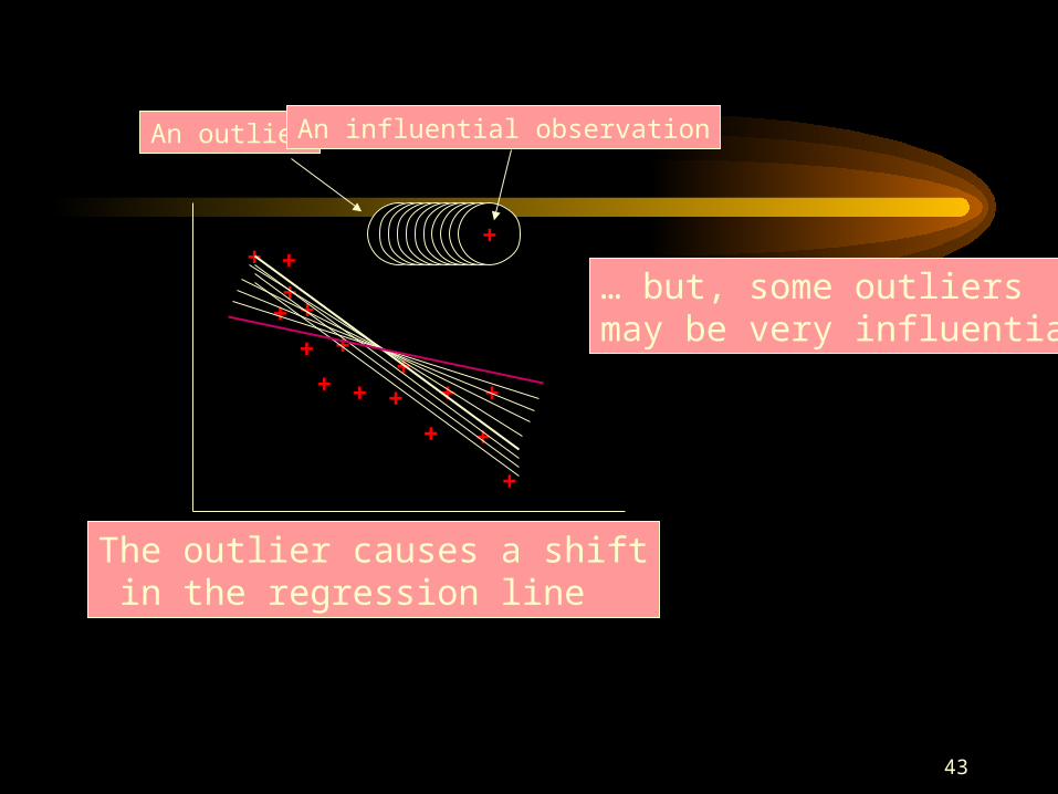
The outlier causes a shift in the regression line

… but, some outliers may be very influential

++++++++++

An outlier An influential observation

44

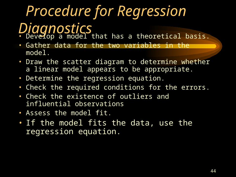
Procedure for Regression Diagnostics• Develop a model that has a theoretical basis.• Gather data for the two variables in the model.• Draw the scatter diagram to determine whether a linear

model appears to be appropriate.• Determine the regression equation.• Check the required conditions for the errors.• Check the existence of outliers and influential observations• Assess the model fit.

• If the model fits the data, use the regression equation.

45

Part II: Experimental Method

46

Outline

• Critique of Regression

47

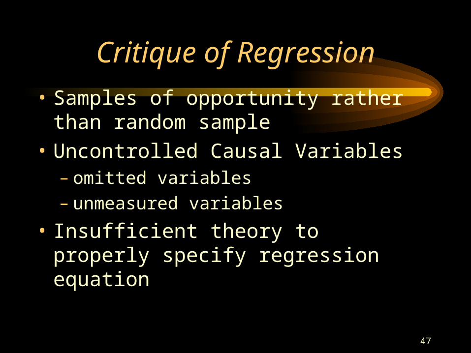
Critique of Regression

• Samples of opportunity rather than random sample

• Uncontrolled Causal Variables– omitted variables– unmeasured variables

• Insufficient theory to properly specify regression equation

48

Experimental Method: # Examples

• Deterrence

• Aspirin

• Miles per Gallon

49

Deterrence and the Death Penalty

50

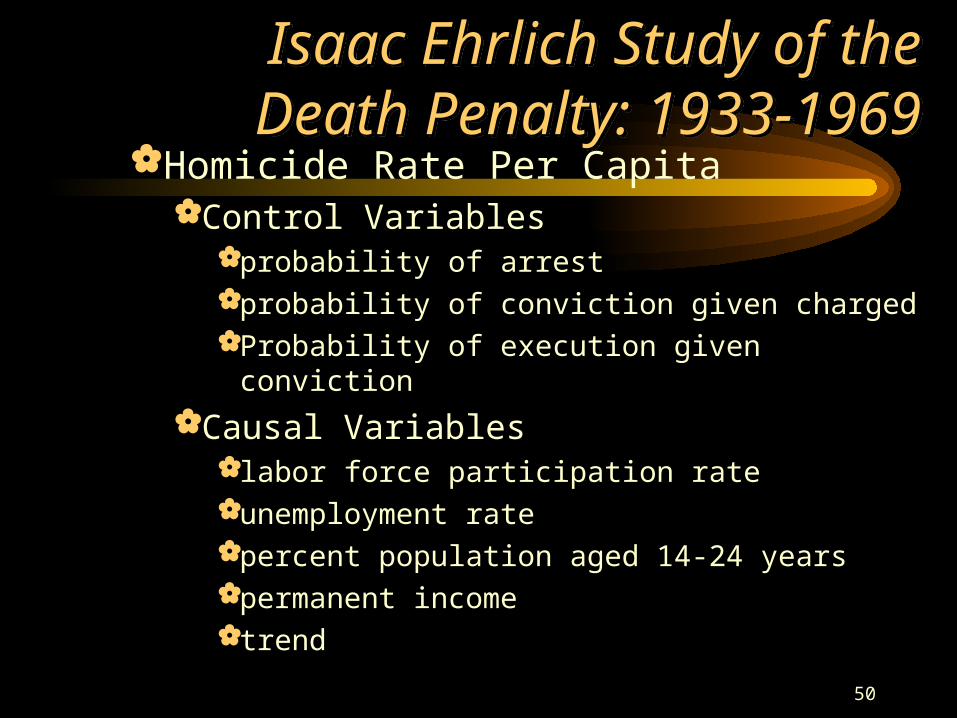
Isaac Ehrlich Study of the Death Penalty: 1933-1969

Isaac Ehrlich Study of the Death Penalty: 1933-1969

Homicide Rate Per CapitaControl Variables

probability of arrestprobability of conviction given charged Probability of execution given conviction

Causal Variableslabor force participation rateunemployment ratepercent population aged 14-24 yearspermanent incometrend

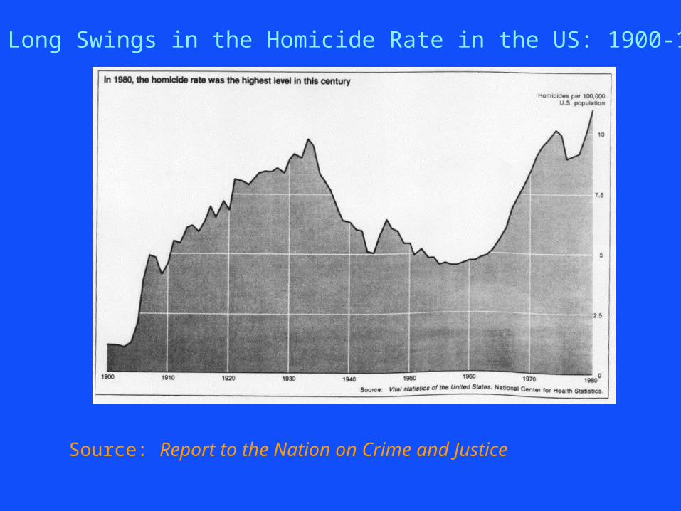
Long Swings in the Homicide Rate in the US: 1900-1980

Source: Report to the Nation on Crime and Justice

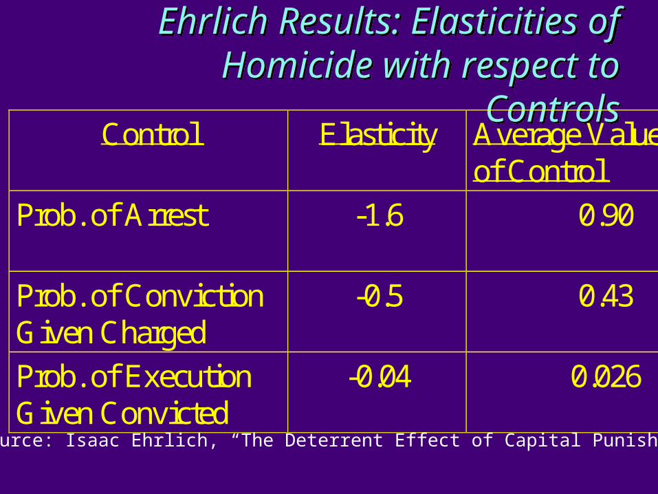
Ehrlich Results: Elasticities of Homicide with respect to Controls

Ehrlich Results: Elasticities of Homicide with respect to Controls

Control Elasticity Average Valueof Control

Prob. of Arrest -1.6 0.90

Prob. of ConvictionGiven Charged

-0.5 0.43

Prob. of ExecutionGiven Convicted

-0.04 0.026

Source: Isaac Ehrlich, “The Deterrent Effect of Capital Punishment

53

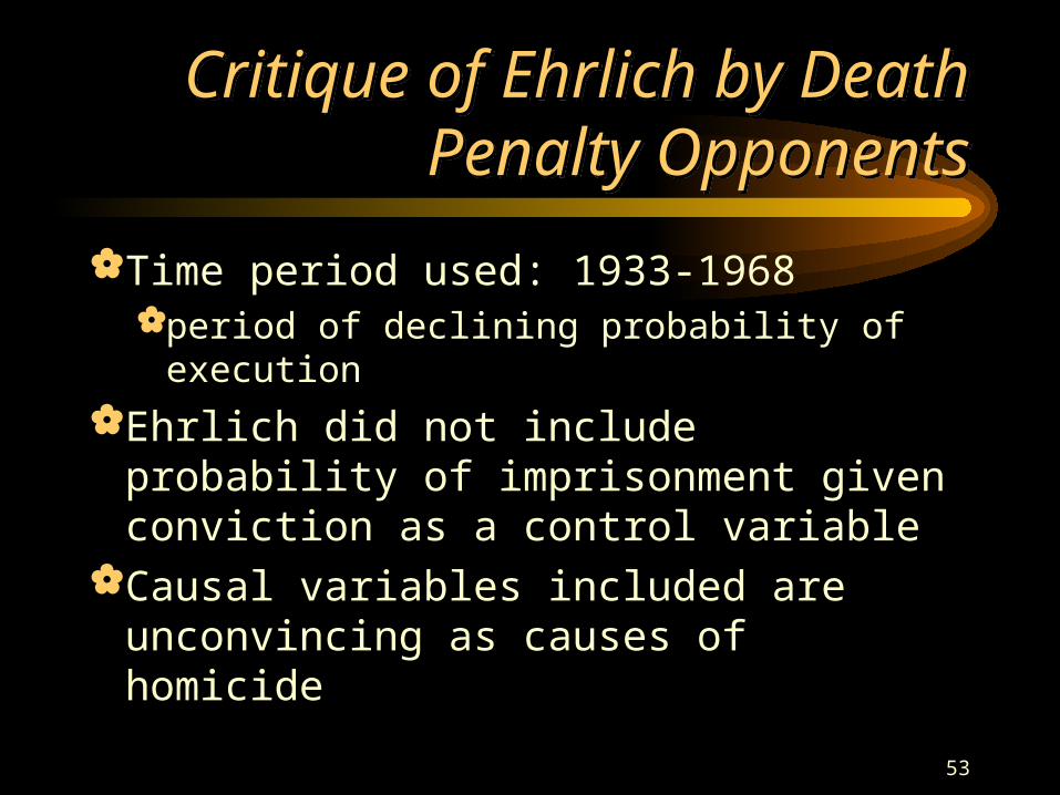
Critique of Ehrlich by Death Penalty Opponents

Critique of Ehrlich by Death Penalty Opponents

Time period used: 1933-1968period of declining probability of execution

Ehrlich did not include probability of imprisonment given conviction as a control variable

Causal variables included are unconvincing as causes of homicide

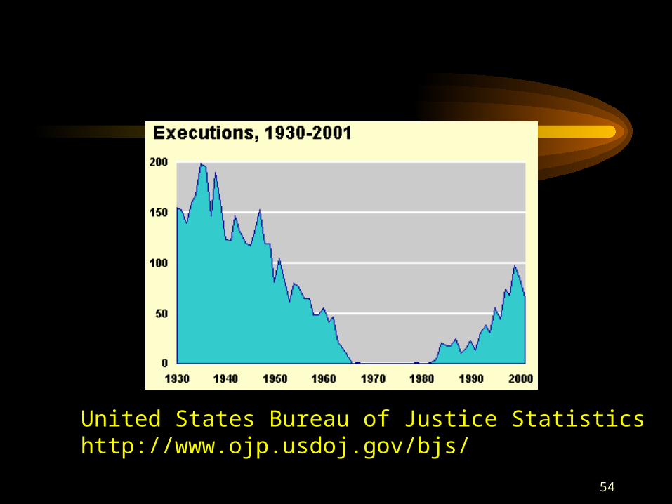
54

United States Bureau of Justice Statisticshttp://www.ojp.usdoj.gov/bjs/

55

Experimental Method

• Police intervention in family violence

56

http://www.ojp.usdoj.gov/bjs/

United States Bureau of Justice Statistics

57

United States Bureau of Justice Statisticshttp://www.ojp.usdoj.gov/bjs/

58

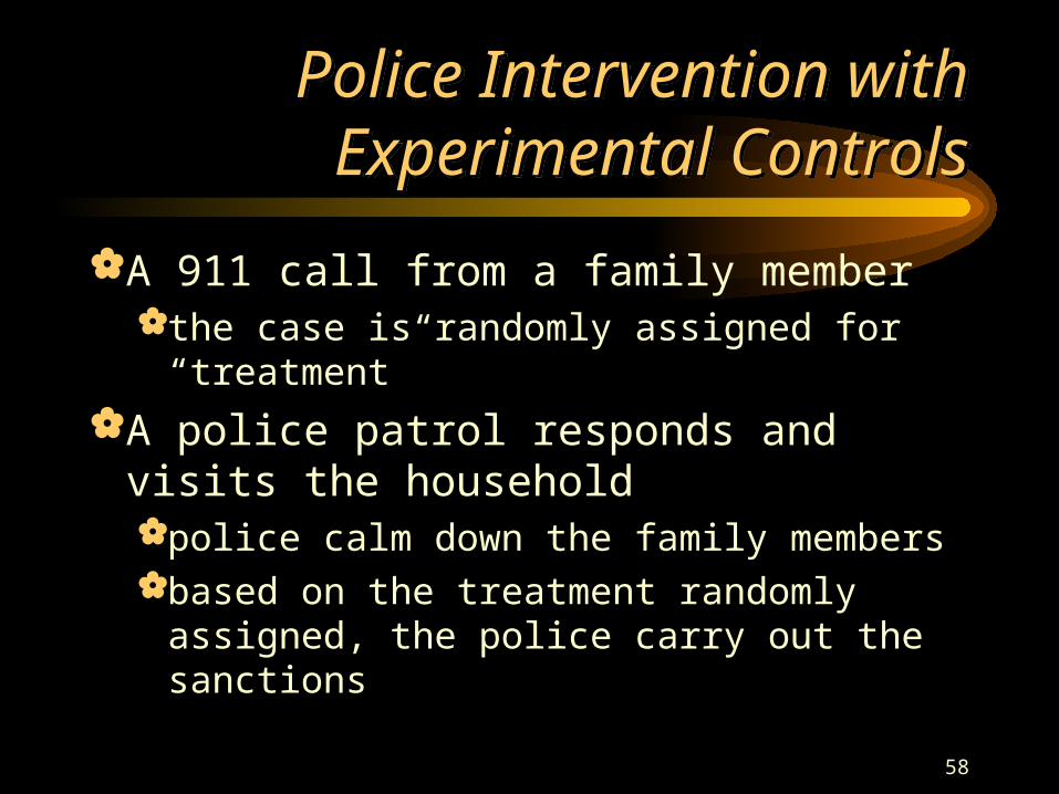
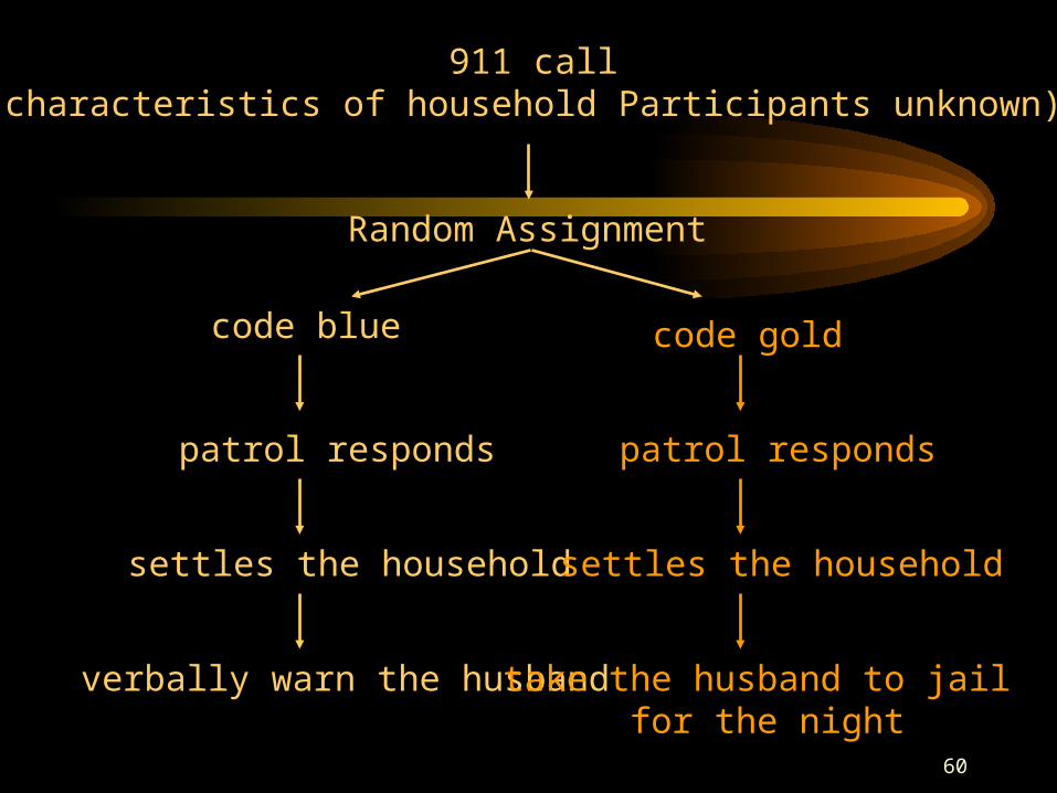
Police Intervention with Experimental Controls

Police Intervention with Experimental Controls

A 911 call from a family memberthe case is randomly assigned for “treatment”

A police patrol responds and visits the householdpolice calm down the family membersbased on the treatment randomly assigned, the

police carry out the sanctions

59

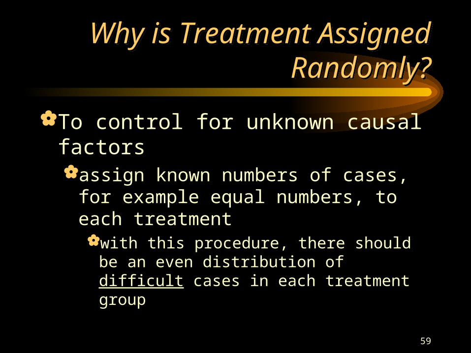
Why is Treatment Assigned Randomly?

Why is Treatment Assigned Randomly?

To control for unknown causal factorsassign known numbers of cases, for example

equal numbers, to each treatmentwith this procedure, there should be an even

distribution of difficult cases in each treatment group

60

911 call(characteristics of household Participants unknown)

Random Assignment

code blue code gold

patrol responds patrol responds

settles the household settles the household

verbally warn the husband take the husband to jail for the night

Power Ten: Conclusion

• Midterm

• Project I

• Experimental Method examples Cont.

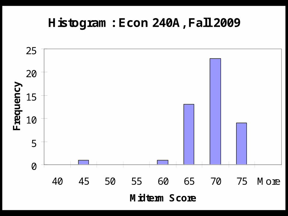
Histogram: Econ 240A, Fall 2009

0

5

10

15

20

25

40 45 50 55 60 65 70 75 More

Midterm Score

Fre

qu

ency

0

4

8

12

16

40 45 50 55 60 65 70 75

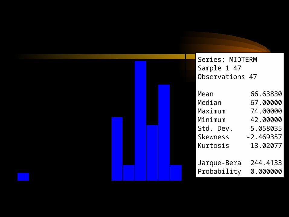
Series: MIDTERMSample 1 47Observations 47

Mean 66.63830Median 67.00000Maximum 74.00000Minimum 42.00000Std. Dev. 5.058035Skewness -2.469357Kurtosis 13.02077

Jarque-Bera 244.4133Probability 0.000000

Econ 240A Midterm Score

0

2

4

6

8

10

60 61 62 63 64 65 66 67 68 69 70 71 72 73 74 75

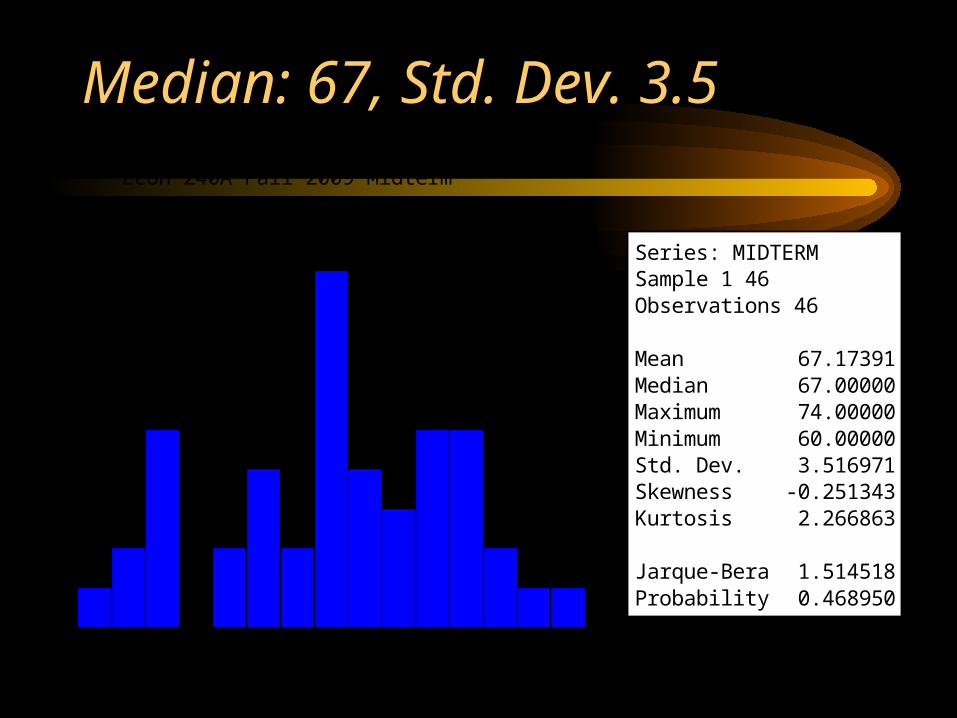
Series: MIDTERMSample 1 46Observations 46

Mean 67.17391Median 67.00000Maximum 74.00000Minimum 60.00000Std. Dev. 3.516971Skewness -0.251343Kurtosis 2.266863

Jarque-Bera 1.514518Probability 0.468950

Econ 240A Fall 2009 Midterm

Median: 67, Std. Dev. 3.5

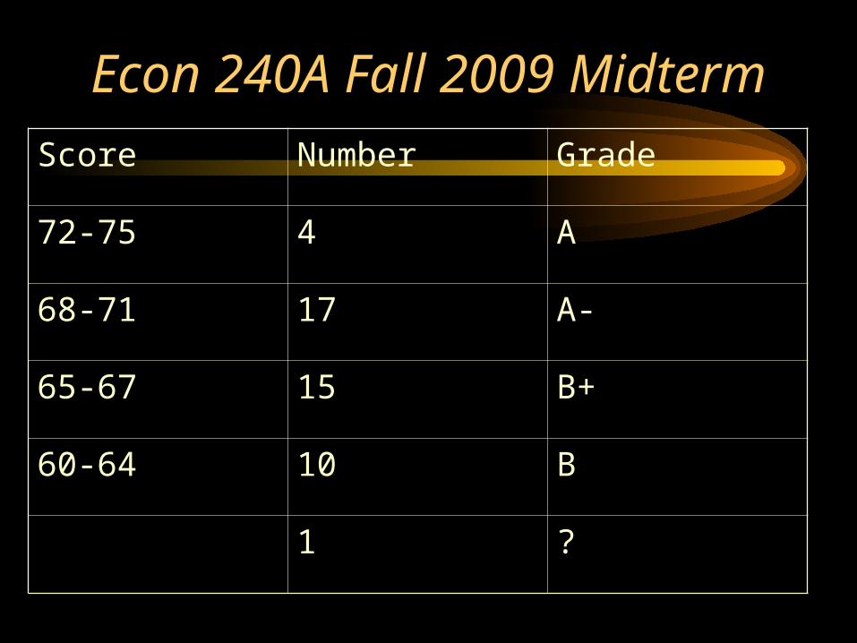
Econ 240A Fall 2009 Midterm

Score Number Grade

72-75 4 A

68-71 17 A-

65-67 15 B+

60-64 10 B

1 ?

70

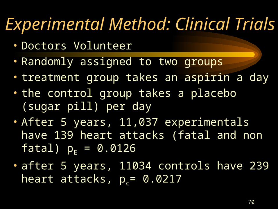
Experimental Method: Clinical Trials• Doctors Volunteer

• Randomly assigned to two groups

• treatment group takes an aspirin a day

• the control group takes a placebo (sugar pill) per day

• After 5 years, 11,037 experimentals have 139 heart attacks (fatal and non fatal) pE = 0.0126

• after 5 years, 11034 controls have 239 heart attacks, pc= 0.0217

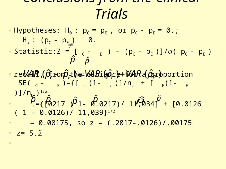
Conclusions from the Clinical Trials• Hypotheses: H0 : pC = pE , or pC - pE = 0.; Ha : (pC -

pE ) 0.

• Statistic:Z = [ C - E ) – (pC - pE )]/( pC - pE )

• recall, from the variance for a proportionSE SE( C -

E )={[ c (1- c )]/nc + [ E(1- E )]/nE }1/2

• { [0.={[0217 ( 1- 0.0217)/ 11,034] + [0.0126 ( 1 – 0.0126)/ 11,039}1/2

• = 0.00175, so z = (.2017-.0126)/.00175• z= 5.2•

pp

p p p p p p

)ˆ()ˆ()ˆˆ( EcEc pVARpVARppVAR

72

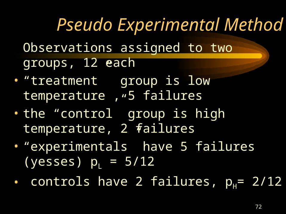
Pseudo Experimental Method Observations assigned to two groups, 12 each

• “treatment” group is low temperature , 5 failures

• the “control” group is high temperature, 2 failures

• “experimentals” have 5 failures (yesses) pL = 5/12

• controls have 2 failures, pH= 2/12

73

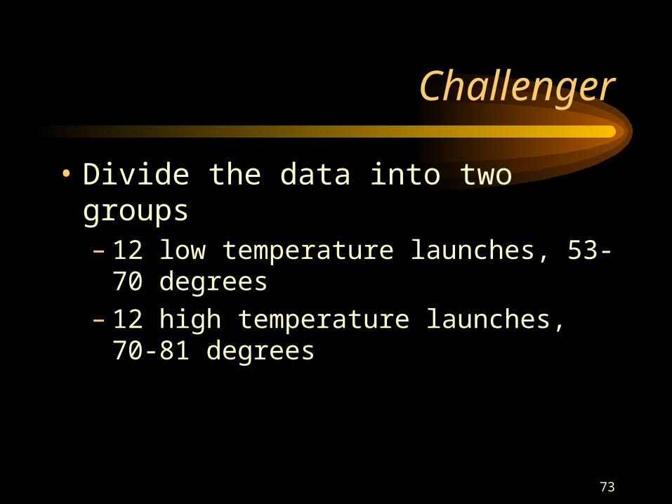
Challenger

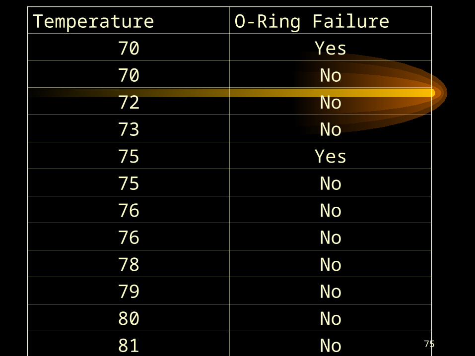
• Divide the data into two groups– 12 low temperature launches, 53-70 degrees– 12 high temperature launches, 70-81 degrees

74

Temperature O-Ring Failure

53 Yes

57 Yes

58 Yes

63 Yes

66 No

67 NO

67 No

67 No

68 No

69 No

70 No

70 Yes

75

Temperature O-Ring Failure

70 Yes

70 No

72 No

73 No

75 Yes

75 No

76 No

76 No

78 No

79 No

80 No

81 No

76

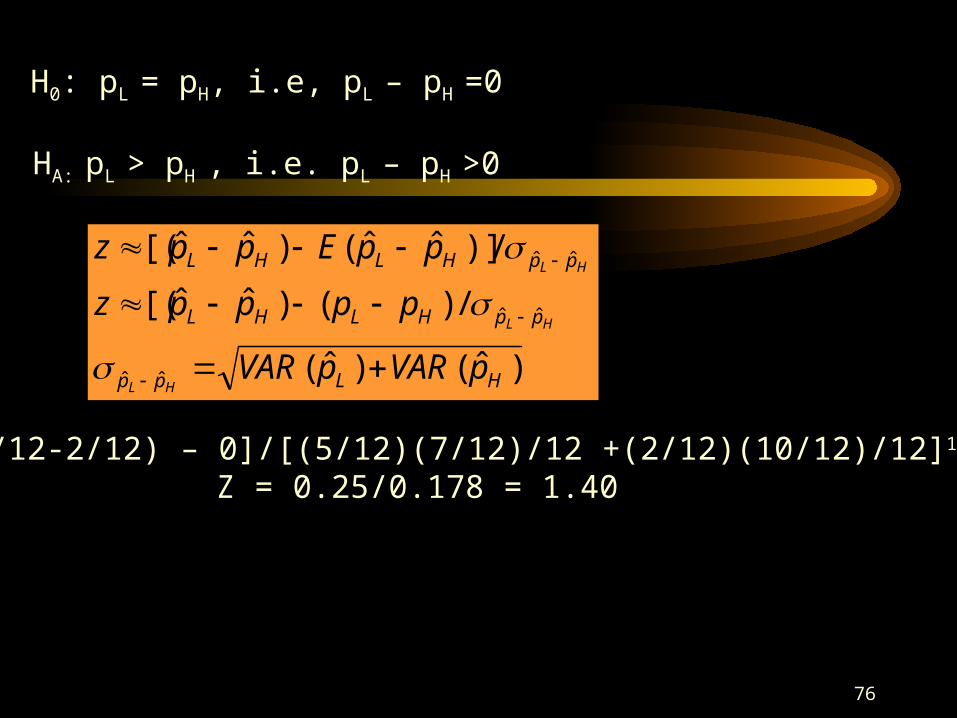
H0: pL = pH, i.e, pL – pH =0

HA: pL > pH , i.e. pL – pH >0

z

ppEppzHL ppHLHL ˆˆ/)ˆˆ()ˆˆ(

)ˆ()ˆ(

/)()ˆˆ[(

/)]ˆˆ()ˆˆ[(

ˆˆ

ˆˆ

ˆˆ

HLpp

ppHLHL

ppHLHL

pVARpVAR

ppppz

ppEppz

HL

HL

HL

Z = [(5/12-2/12) – 0]/[(5/12)(7/12)/12 +(2/12)(10/12)/12]1/2

Z = 0.25/0.178 = 1.40

77

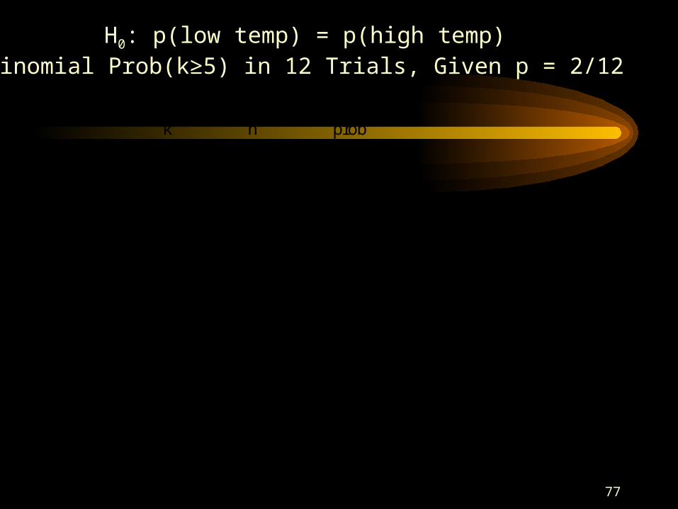
k n prob0 12 0.1121571 12 0.2691762 12 0.2960943 12 0.1973964 12 0.0888285 12 0.028425 0.0284249836 12 0.006632 0.0350574797 12 0.001137 0.0361944788 12 0.000142 0.0363366039 12 1.26E-05 0.036349236

10 12 7.58E-0711 12 2.76E-0812 12 4.59E-10

H0: p(low temp) = p(high temp) Binomial Prob(k≥5) in 12 Trials, Given p = 2/12

78

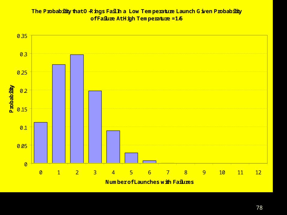
The Probability that O-Rings Fail In a Low Temperature Launch Given Probability of Failure At High Temperature =1/6

0

0.05

0.1

0.15

0.2

0.25

0.3

0.35

0 1 2 3 4 5 6 7 8 9 10 11 12

Number of Launches with Failures

Pro

bab

ility

79

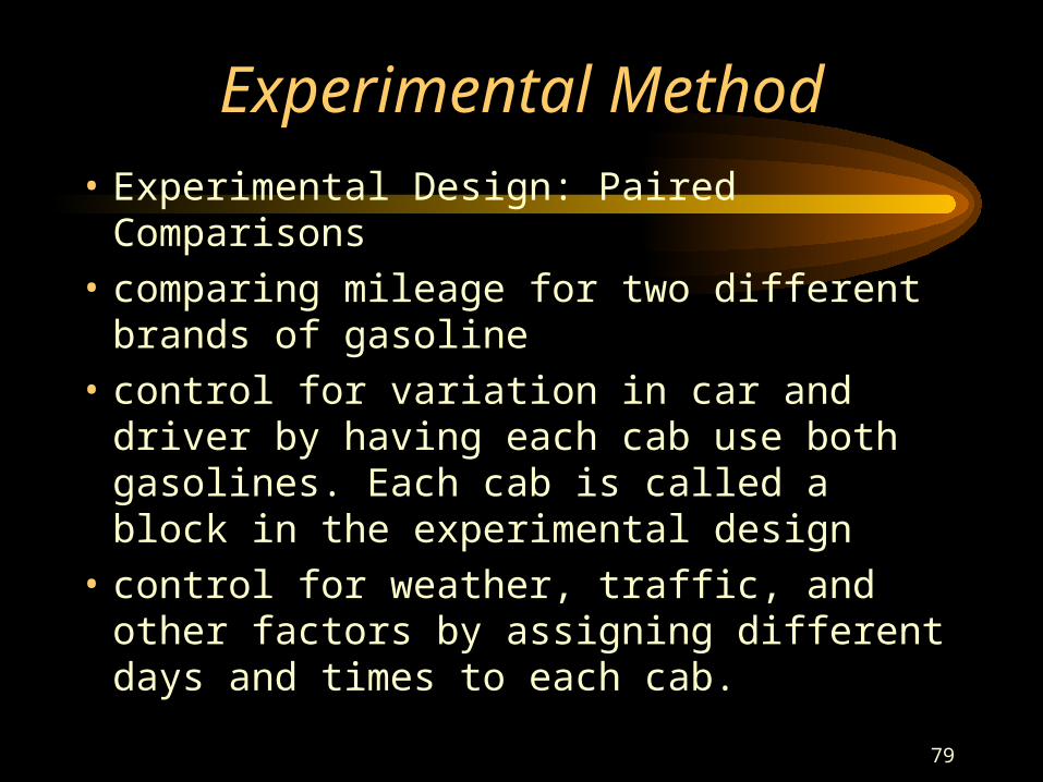
Experimental Method

• Experimental Design: Paired Comparisons

• comparing mileage for two different brands of gasoline

• control for variation in car and driver by having each cab use both gasolines. Each cab is called a block in the experimental design

• control for weather, traffic, and other factors by assigning different days and times to each cab.

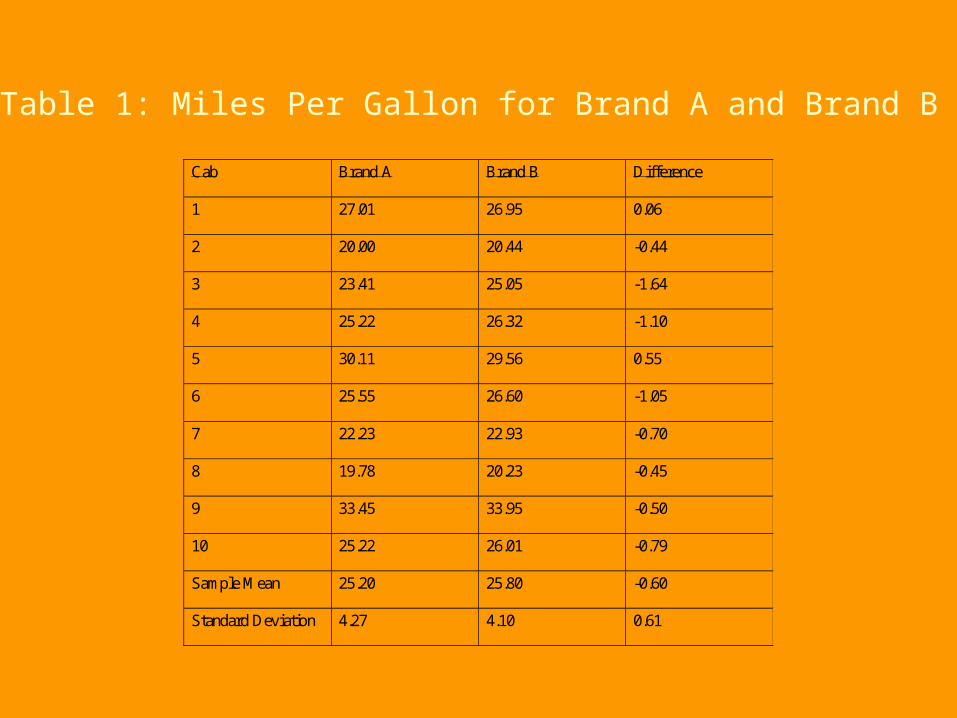
Cab Brand A Brand B Difference

1 27.01 26.95 0.06

2 20.00 20.44 -0.44

3 23.41 25.05 -1.64

4 25.22 26.32 -1.10

5 30.11 29.56 0.55

6 25.55 26.60 -1.05

7 22.23 22.93 -0.70

8 19.78 20.23 -0.45

9 33.45 33.95 -0.50

10 25.22 26.01 -0.79

Sample Mean 25.20 25.80 -0.60

Standard Deviation 4.27 4.10 0.61

Table 1: Miles Per Gallon for Brand A and Brand B

81

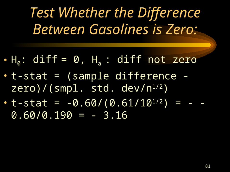
Test Whether the Difference Between Gasolines is Zero:

• H0: diff = 0, Ha : diff not zero

• t-stat = (sample difference - zero)/(smpl. std. dev/n1/2)

• t-stat = -0.60/(0.61/101/2) = - -0.60/0.190 = - 3.16

82

83

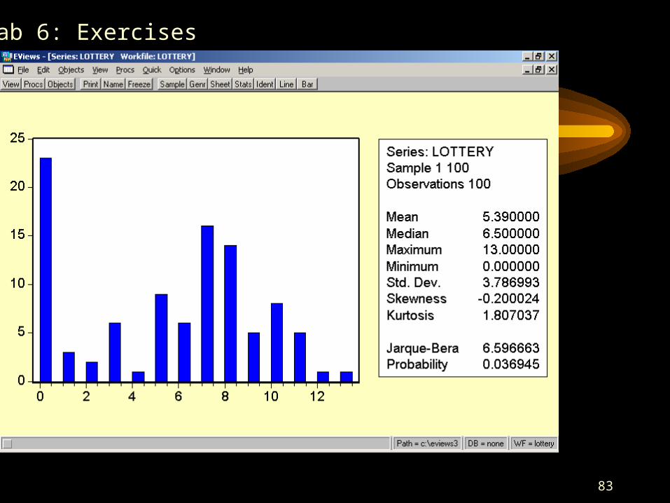
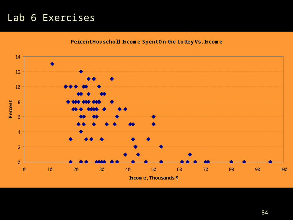
Lab 6: Exercises

84

Percent Household Income Spent On the Lottey Vs. Income

0

2

4

6

8

10

12

14

0 10 20 30 40 50 60 70 80 90 100

Income, Thousands $

Per

cen

t

Lab 6 Exercises

85

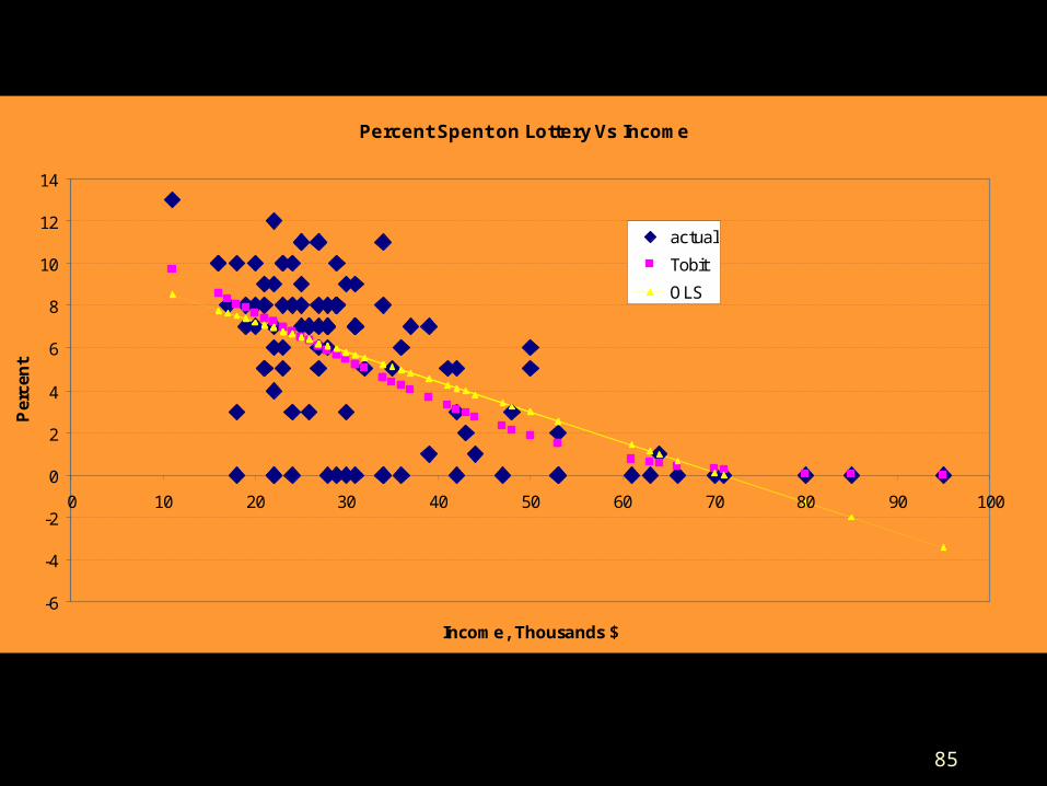
Percent Spent on Lottery Vs Income

-6

-4

-2

0

2

4

6

8

10

12

14

0 10 20 30 40 50 60 70 80 90 100

Income, Thousands $

Per

cen

t

actual

Tobit

OLS

86

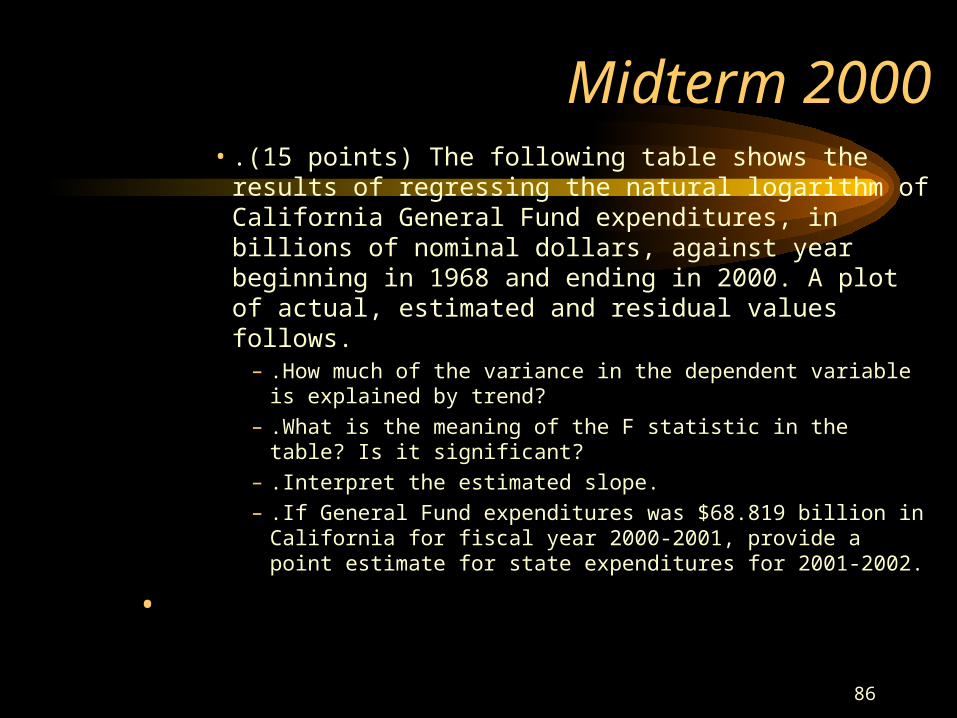
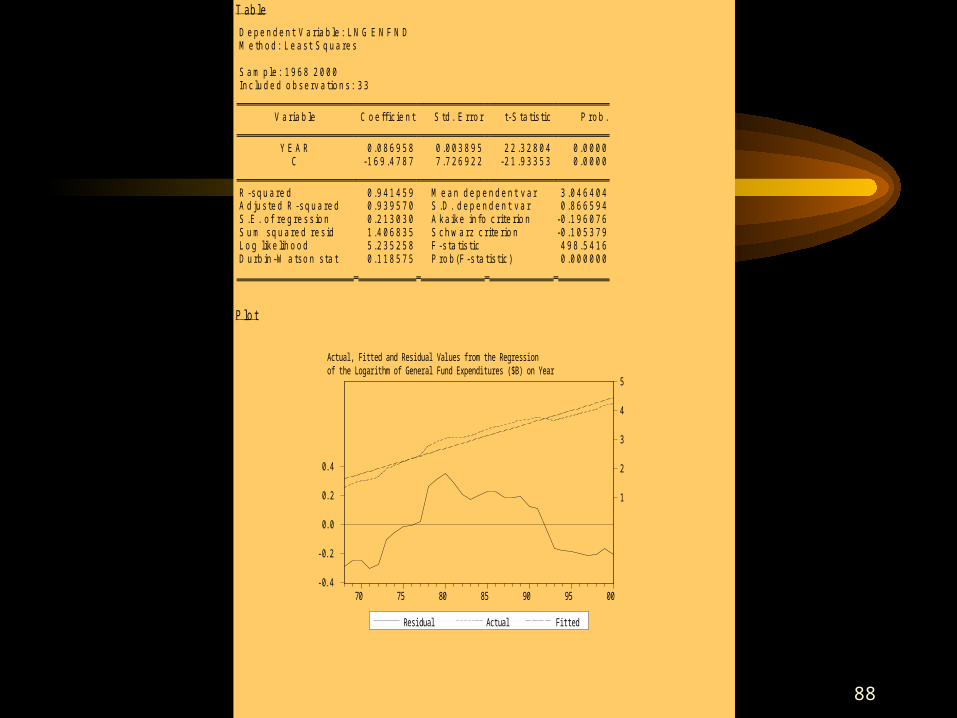
Midterm 2000• .(15 points) The following table shows the results of

regressing the natural logarithm of California General Fund expenditures, in billions of nominal dollars, against year beginning in 1968 and ending in 2000. A plot of actual, estimated and residual values follows.

– .How much of the variance in the dependent variable is explained by trend?

– .What is the meaning of the F statistic in the table? Is it significant?

– .Interpret the estimated slope.

– .If General Fund expenditures was $68.819 billion in California for fiscal year 2000-2001, provide a point estimate for state expenditures for 2001-2002.

•

87

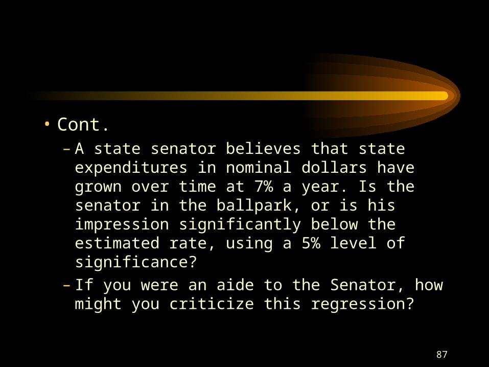
• Cont.– A state senator believes that state expenditures

in nominal dollars have grown over time at 7% a year. Is the senator in the ballpark, or is his impression significantly below the estimated rate, using a 5% level of significance?

– If you were an aide to the Senator, how might you criticize this regression?

88

T a b l e

D e p e n d e n t V a r i a b l e : L N G E N F N DM e t h o d : L e a s t S q u a r e s

S a m p l e : 1 9 6 8 2 0 0 0I n c l u d e d o b s e r v a t i o n s : 3 3

V a r i a b l e C o e f f i c i e n t S t d . E r r o r t - S t a t i s t i c P r o b .

Y E A R 0 . 0 8 6 9 5 8 0 . 0 0 3 8 9 5 2 2 . 3 2 8 0 4 0 . 0 0 0 0C - 1 6 9 . 4 7 8 7 7 . 7 2 6 9 2 2 - 2 1 . 9 3 3 5 3 0 . 0 0 0 0

R - s q u a r e d 0 . 9 4 1 4 5 9 M e a n d e p e n d e n t v a r 3 . 0 4 6 4 0 4A d j u s t e d R - s q u a r e d 0 . 9 3 9 5 7 0 S . D . d e p e n d e n t v a r 0 . 8 6 6 5 9 4S . E . o f r e g r e s s i o n 0 . 2 1 3 0 3 0 A k a i k e i n f o c r i t e r i o n - 0 . 1 9 6 0 7 6S u m s q u a r e d r e s i d 1 . 4 0 6 8 3 5 S c h w a r z c r i t e r i o n - 0 . 1 0 5 3 7 9L o g l i k e l i h o o d 5 . 2 3 5 2 5 8 F - s t a t i s t i c 4 9 8 . 5 4 1 6D u r b i n - W a t s o n s t a t 0 . 1 1 8 5 7 5 P r o b ( F - s t a t i s t i c ) 0 . 0 0 0 0 0 0

P lo t

-0.4

-0.2

0.0

0.2

0.4

1

2

3

4

5

70 75 80 85 90 95 00

Residual Actual Fitted

Actual, Fitted and Residual Values from the Regressionof the Logarithm of General Fund Expenditures ($B) on Year