Embed Size (px)
Citation preview
1
MAN 702
MANAGERIAL FINANCE
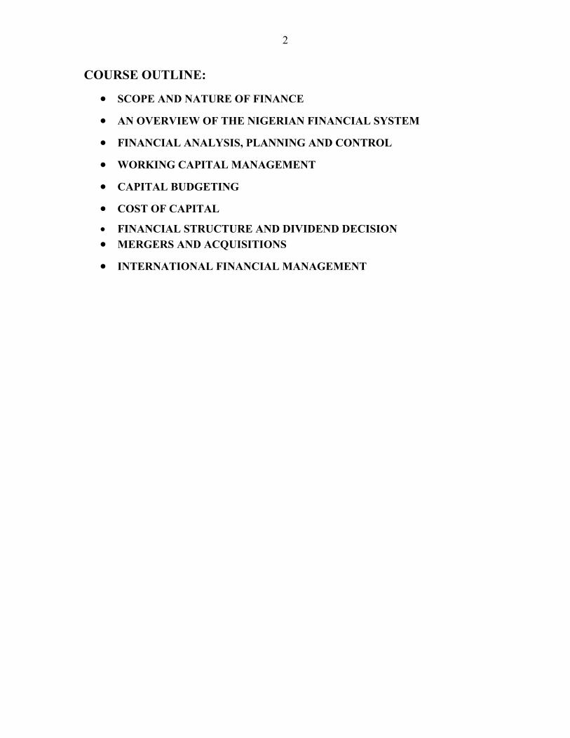
2
COURSE OUTLINE:
SCOPE AND NATURE OF FINANCE
AN OVERVIEW OF THE NIGERIAN FINANCIAL SYSTEM
FINANCIAL ANALYSIS, PLANNING AND CONTROL
WORKING CAPITAL MANAGEMENT
CAPITAL BUDGETING
COST OF CAPITAL
FINANCIAL STRUCTURE AND DIVIDEND DECISION
MERGERS AND ACQUISITIONS
INTERNATIONAL FINANCIAL MANAGEMENT
3
SCOPE AND NATURE OF FINANCE
Meaning of Financial Management
The Finance Function
Finance in the organisation structure of the firm
Goals of the firm
(a) Meaning of Financial Management
Financial management is simply explained as the management of the finance of a
business. That is, applying management functions such as planning and control in order
to achieve the financial objectives of the business.
It is that managerial activity which is concerned with the planning and controlling of the
firm’s financial resources.
As a separate discipline, it is a recent development because up till 1890, it was a branch
of economics. Until today, it has no unique body of knowledge of its own, and it draws
heavily on economics for its theoretical concepts.
(b) The Finance Function
Viewing an organisation from functional perspective presents an organisation comprising
of various functional areas among which are finance, production and marketing. The
company (firm) secures capital it needs and employs it (finance activity) in activities
which generate returns on invested capital (production and marketing activities). A
business organisation therefore engages in activities to perform functions such as those
discussed above; Finance, production and marketing. The most important of these is the
finance function. The finance function is so important that all organisations perform
them. There is ranging from business firms to government units or agencies and other
non-profit organisations. Finance function has to do with the financial management,
which is defined, by the functions and areas of responsibilities of financial managers.
4
The functions of financial managers are broadly appreciated under the following
activities
(i) Planning and Forecasting
The financial manager has to set financial objectives and work toward achieving such
predetermined target. Thus, setting a realistic target requires making educative guesses
about the future based on the past and present information. Areas of concern here include
planning for working capital components, capital budgeting etc.
(ii) Investment and Financing Decision
The financial manager has the primary responsibility for: (a) acquiring funds, which are
obtained from a wide range of financial institutions; (b) Determining a sound rate of
growth and ranking alternative investment opportunities to ensure that the firm achieves a
high rate of growth in sales (c) Deciding the specific investment to be made and
alternative sources of funds for financing these investments; (d) Deciding about the use
of internal vs. external funds, of debt vs. owner’s funds, and of long term vs. short-term
financing; and (e) Should be concerned with the management of cash inflows (in form
of retained earnings) and cash outflows (in form of dividends) since some cash is
recycled and some returned to financing sources.
(iii) Interaction with Other Managers in the firm. Since all business decisions have
financial implications.
(iv). Using money and capital markets.
According to Weston and Copeland (1989:33) financial managers have two important
areas of responsibility:
To obtain external funds through the financial markets.
What financing forms and sources are available?
How can the funds be acquired efficiently?
What is the most economical mix of financing?
What will be the timing and form of returns and repayments to financing
sources?

5
To see that the funds obtained are used effectively.
To what projects and products should funds be allocated?
What assets and resources must be acquired in order to produce the product or
service?
How should the use of funds be monitored so that they are most effectively
distributed among the various operating activities?
It is the financial manager’s responsibility to implement these choices in the various
financial markets to meet the firm’s capital requirements
(c) Finance in the Organisation Structure of the Firm
The place of the Chief Financial Officer (CFO) is high in the organisational hierarchy of
the firm because of the central role of finance in the various levels of decision-making.
The organisational structure below shows the position of the CFO.
CHAIRMAN OF THE BOARD
MANAGING DIRECTOR
BOARD
RESEARCH DIRECTOR
PRODUCTION DIRECTOR
MARKETING DIRECTOR
FINANCIAL DIRECTOR
(CFO)
CONTROLLER TREASURER
6
Chief Financial Officer (C F O)
Is responsible for formulation of major financial policies in the firm.
Interact with other senior officers to present the financial implications of
major decisions in other areas.
Defines the duties of other financial officers who report to him.
Is accountable for the analytical aspects of the treasurer and controller’s
activities.
The Treasurer: handles the acquisition and custody of funds. In addition he also
handles
Forecasting and financial needs.
Banking and custody
Credits and collections
Investments
Insurance
Controller: his areas of responsibility include:
Accounting
Reporting
Control/Government’s reporting and
Protection of Assets
(d) Goals of the Firm
The firm’s investment and financing decisions are unavoidable and continuous. In order
to make them rationally, the firm must have a goal. It is generally agreed however, that
the financial goal of the firm should be the maximisation of owner’s economic welfare.
The three major goals of the firm discussed in literature are: profit maximization;
shareholders’ wealth maximization; and social responsibility.
(i) Profit Maximisation:-This goal is to increase the firm’s Naira earnings to as large an
amount as possible, usually in as short a time as possible.
7
- This goal has the advantage of focusing the firm’s effort on profits, which are
absolute necessity for the company’s continued independent existence.
- However, the firm can suffer if the profit maximisation goal is taken to extremes.
This is because of the following reasons:
(a) Pursuit of profits alone can lead to poor risk judgment.
(b) An emphasis on short-term profits can cause the neglect of long-term
possibilities.
(c) The firm’s managers, especially in a corporation, may be willing to
undertake the risks essential to profit maximisation.
(d) Capital and other resources may be insufficient to take advantage of
immediate opportunities.
(ii) Shareholders’ wealth maximisation
- This goal stresses the maximisation of the market value of the firm (Maximising
the price of the firm’s ordinary shares) and hence the wealth of its shareholders.
- In finance, this goal is seen as the critically logical and operationally feasible
normative goal for guiding the financial decision-making.
- This corporate goal should reflect all favourable as well as unfavourable factors
affecting the firm.
- The wealth of the shareholders is increased when the share price goes up. The
share price reflects:
Management’s performance is achieving earnings.
Their ability to judge risks and
Factors outside the firm’s control to which investors respond e.g. interest rate.
The wealth maximisation goal is consistent with the objective of maximising
owner’s economic welfare. The latter is equivalent to maximising the utility of
their consumption over-time. With their wealth maximised, owners can adjust
their cash flows in such a way as to optimise their consumption.
- Value maximisation is therefore broader than profit maximisation for several
reasons:-
8
(i) Maximisation of value takes the time value of money into consideration.
Funds received this year have more value than funds that may be received ten
years later.
(ii) Value maximisation considers the risk-ness of the income streams, e.g. the
rate of return required on risk-free government securities would be lower than
the rate of return required on an investment in starting a new business.
(iii) Social Responsibility
This is a new concept which is now in vogue. -It stresses that business should not strictly
operate in shareholders’ best interest but should partly be responsible for the welfare of
society. There is no one, and especially large firm, that can afford to ignore obligations
for responsible citizenship.
9
AN OVERVIEW OF NIGERIAN FINANCIAL SYSTEM
Definition:
A financial system comprises the entire conglomerate of institutions and institutional
arrangements established to serve the needs of modern economies.
(a) It ensures the provision of financial resources to meet the borrowing needs of
individuals, business enterprises and government.
(b) It provides facilities to collect and to invest savings and a sound payment
mechanism.
History
- Before independence, indigenous financial system was almost non-existing. Only
the traditional financial institutions and some few modern but colonial financial
institutions existed whose main objective was to mobilise local savings and
channel them for the sustenance of the metropolitan country’s economy.
- Roots of modern and indigenous financial system – political independence in the
West African countries. First major step was the establishment of CBN in March
1958 under CBN Ordinance 1958. Later series of banks, (commercial and
merchants), non-banks financial institutions and financial markets were
established.
Classification:
One way of identifying or classifying the Nigerian Financial system is by generic names
of the institutions. Thus, we have four major classifications:
1. The Apex Institutions:
(a) CBN - This is at the apex of the banking system.
(b) NSEC - This is the apex of the financial particularly capital markets.
(c) NDIC – This is concerned with insuring all the commercial and merchant
banks i.e. all deposit financed financial institutions.
2. The Banking Institutions
(a) National Development Banks
(b) The Commercial Banks
(c) The Merchant Banks
10
3. The Non-Bank Financial Institutions
(a) Various State Development Financial Institutions
(b) Insurance Companies
(c) Pension Funds
(d) Provident Funds
4. Financial Markets
Money
Capital Markets
11
FINANCIAL ANALYSIS, PLANNING, AND CONTROL FINANCIAL ANALYSIS
- Financial analysis is defined as the process of identifying the financial strengths
and weaknesses of the organisation by properly establishing the relationships
between the various items in the organisations financial statements.
- Financial statements are the results of the process of recording, classifying and
summarising a firm’s transactions.
- Of special interest to financial managers and financial analyst are the Balance
Sheet and the Income Statement that provide a measure of the firm’s financial
condition.
Steps in Financial Statement Analysis:
(i) Select the information relevant to the decision under consideration from the
total information contained in the financial statements
(ii) Arrange the information in a way as to highlight significant relationship.
(iii) The acquired information is to be interpreted, inference and conclusions
drawn.
Users of Financial Statement:
(i) Creditors i.e. short-term and long -term.
(ii) Shareholders and potential investors
(iii) Labour Unions – i.e. justifying wage increase and other welfare services.
(iv) Competitors
(v) Management analysts
Financial Ratio Analysis
- It is a widely used tool of financial analysis
- It is used as an index or yardstick for evaluating the financial position and
performance in finance.
12
Basic Types of Financial Ratios
(a) Liquidity Ratios: Measure the short-term solvency of the firm.
(b) Gearing /Capital Structure/Leverage/Debt Ratios: They measure the extent to
which the firm’s assets are financed by debt and firm’s ability to meet long-term
commitments.
(c) Activity Ratios: They measure the overall effectiveness of financial utilisation i.e.
ability of a firm to manage and utilize its asset.
(d) Profitability Ratios: These provide a measure of profitability to firm.
(e) Growth Ratios: These ratios measure how well the firm is maintaining its
economic position in the economy as a whole as well as its own industry.
(f) Valuation Ratios: These are the most comprehensive measures of performance for
the firm in that they reflect the combined influence of risk ratios and return ratios.
General Uses/Advantages
(i) They explain the ability of the firm to meet the financial obligation when they
fall due.
(ii) They aid decision making by summarising, simplifying and classifying
accounting records.
(iii) Yardstick for measuring performance
(iv) Used for the purpose of comparison
Limitations:
Although they are important and useful, they must be used with caution because:
(a) There is a high chance of window- dressing technique in which published data are
presented to outside users.
(b) Differences in accounting systems e.g. depreciation methods.
(c) Impact of inflation
(d) Conceptual Differences e.g. what constitutes shareholders’ equity or using the
value of sales or cost of goods sold in the computation of the turnover ratios.
FINANCIAL RATIOS AS PREDICTIONS OF CORPORATE FAILURE
- The ratios are tools of analysing financial record i.e. its strengths and weaknesses,
depending on who the user is.
13
- One serious shortcoming of ratio analysis arises from the fact that the
methodology is univariate i.e. each ratio is examined in isolation.
- To overcome this univariate position, it is necessary to put together different
ratios into a meaningful predictive model.
- So many people attempted a predictive model and their contributions are
discussed below:
William Beaver:
- Made first attempt in 1966 to develop a univariate model
- Wrote on “Financial ratios and predictors of Failure”
- He was interested in finding out which ratios are most important in predicting a
firm’s inability to pay its debts.
- He compared the ratios of 79 firms and another 79 firms. The former failed and
the latter solvent.
- He found that there are five (5) key ratios that could discriminate between a firm
that failed and the firm that survived. These ratios are:
(1) The Cash flow to Total Debt
(2) Net Income to Total Asset
(3) Total Debt to Total Asset
(4) Working capital to Total Asset
(5) Current- Ratio.
- He found that all firms that failed had more debt, lower return on assets, less cash
balances, more receivable and low current ratios.
Altman Edward:
- He uses the Discriminant Analysis to develop a multivariate model.
- He developed a model of predicting bankruptcy of firms in U.S. (Financial Ratio
Discriminant analysis and prediction of corporate bankruptcy)
- He used a sample of 66 manufacturing firms. Half of which went bankruptcy.
- From their financial statements one period before the bankrupt, he discovered 22
financial ratios out of which five were found to contribute immensely to the
prediction model.
14
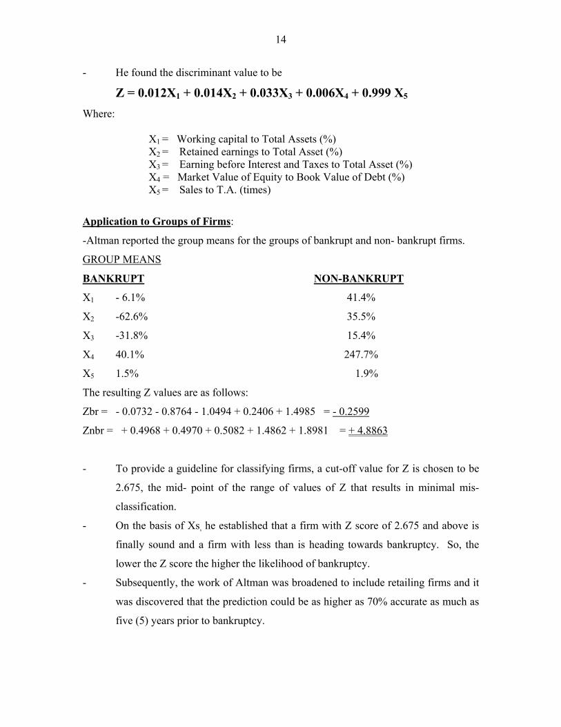
- He found the discriminant value to be
Z = 0.012X1 + 0.014X2 + 0.033X3 + 0.006X4 + 0.999 X5
Where:
X1 = Working capital to Total Assets (%) X2 = Retained earnings to Total Asset (%) X3 = Earning before Interest and Taxes to Total Asset (%) X4 = Market Value of Equity to Book Value of Debt (%) X5 = Sales to T.A. (times)
Application to Groups of Firms:
-Altman reported the group means for the groups of bankrupt and non- bankrupt firms.
GROUP MEANS
BANKRUPT NON-BANKRUPT
X1 - 6.1% 41.4%
X2 -62.6% 35.5%
X3 -31.8% 15.4%
X4 40.1% 247.7%
X5 1.5% 1.9%
The resulting Z values are as follows:
Zbr = - 0.0732 - 0.8764 - 1.0494 + 0.2406 + 1.4985 = - 0.2599
Znbr = + 0.4968 + 0.4970 + 0.5082 + 1.4862 + 1.8981 = + 4.8863
- To provide a guideline for classifying firms, a cut-off value for Z is chosen to be
2.675, the mid- point of the range of values of Z that results in minimal mis-
classification.
- On the basis of Xs, he established that a firm with Z score of 2.675 and above is
finally sound and a firm with less than is heading towards bankruptcy. So, the
lower the Z score the higher the likelihood of bankruptcy.
- Subsequently, the work of Altman was broadened to include retailing firms and it
was discovered that the prediction could be as higher as 70% accurate as much as
five (5) years prior to bankruptcy.
15
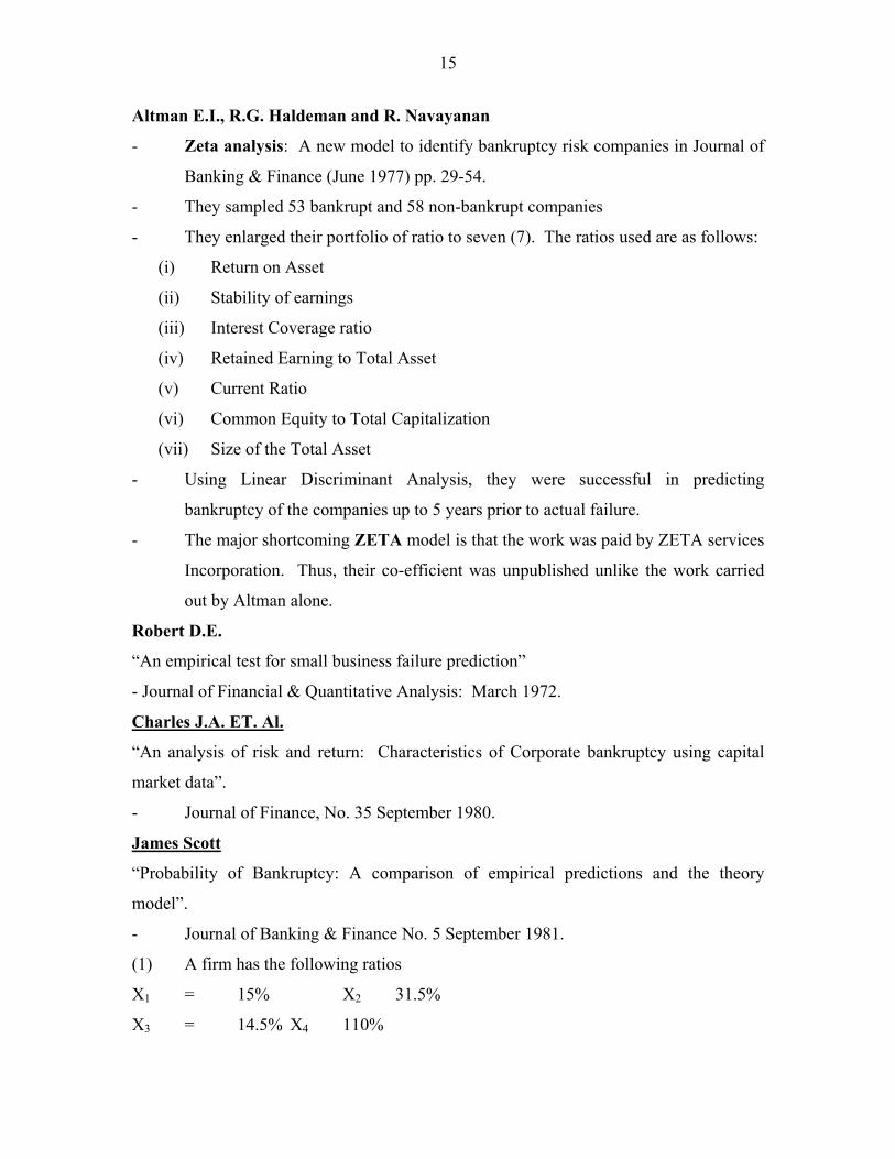
Altman E.I., R.G. Haldeman and R. Navayanan
- Zeta analysis: A new model to identify bankruptcy risk companies in Journal of
Banking & Finance (June 1977) pp. 29-54.
- They sampled 53 bankrupt and 58 non-bankrupt companies
- They enlarged their portfolio of ratio to seven (7). The ratios used are as follows:
(i) Return on Asset
(ii) Stability of earnings
(iii) Interest Coverage ratio
(iv) Retained Earning to Total Asset
(v) Current Ratio
(vi) Common Equity to Total Capitalization
(vii) Size of the Total Asset
- Using Linear Discriminant Analysis, they were successful in predicting
bankruptcy of the companies up to 5 years prior to actual failure.
- The major shortcoming ZETA model is that the work was paid by ZETA services
Incorporation. Thus, their co-efficient was unpublished unlike the work carried
out by Altman alone.
Robert D.E.
“An empirical test for small business failure prediction”
- Journal of Financial & Quantitative Analysis: March 1972.
Charles J.A. ET. Al.
“An analysis of risk and return: Characteristics of Corporate bankruptcy using capital
market data”.
- Journal of Finance, No. 35 September 1980.
James Scott
“Probability of Bankruptcy: A comparison of empirical predictions and the theory
model”.
- Journal of Banking & Finance No. 5 September 1981.
(1) A firm has the following ratios
X1 = 15% X2 31.5%
X3 = 14.5% X4 110%
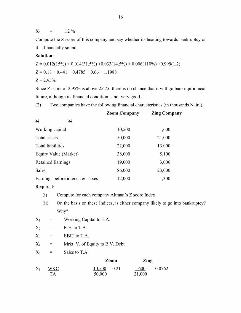
16
X5 = 1.2 %
Compute the Z score of this company and say whether its heading towards bankruptcy or
it is financially sound.
Solution:
Z = 0.012(15%) + 0.014(31.5%) +0.033(14.5%) + 0.006(110%) +0.999(1.2)
Z = 0.18 + 0.441 + 0.4785 + 0.66 + 1.1988
Z = 2.95%
Since Z score of 2.95% is above 2.675, there is no chance that it will go bankrupt in near
future, although its financial condition is not very good.
(2) Two companies have the following financial characteristics (in thousands Naira).
Zoom Company Zing Company
N N
Working capital 10,500 1,600
Total assets 50,000 21,000
Total liabilities 22,000 13,000
Equity Value (Market) 38,000 5,100
Retained Earnings 19,000 3,000
Sales 86,000 23,000
Earnings before interest & Taxes 12,000 1,300
Required:
(i) Compute for each company Altman’s Z score Index.
(ii) On the basis on these Indices, is either company likely to go into bankruptcy?
Why?
X1 = Working Capital to T.A.
X2 = R.E. to T.A.
X3 = EBIT to T.A.
X4 = Mrkt. V. of Equity to B.V. Debt
X5 = Sales to T.A.
Zoom Zing
X1 = WKC 10,500 = 0.21 1,600 = 0.0762 TA 50,000 21,000
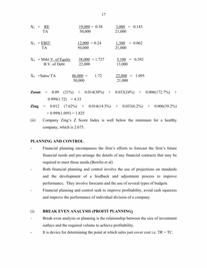
17
X2 = RE 19,000 = 0.38 3,000 = 0.143 TA 50,000 21,000
X3 = EBIT 12,000 = 0.24 1,300 = 0.062 TA 50,000 21,000
X4 = Mrkt V. of Equity 38,000 = 1.727 5,100 = 0.392 B.V. of Debt 22,000 13,000
X5 =Sales⁄ TA 86,000 = 1.72 23,000 = 1.095 50,000 21,000
Zoom = 0.09 (21%) + 0.014(38%) + 0.033(24%) + 0.006(172.7%) +
0.999(1.72) = 4.33
Zing = 0.012 (7.62%) + 0.014(14.3%) + 0.033(6.2%) + 0.006(39.2%)
+ 0.999(1.095) = 1.825
(ii) Company Zing’s Z Score Index is well below the minimum for a healthy
company, which is 2.675.
PLANNING AND CONTROL
- Financial planning encompasses the firm’s efforts to forecast the firm’s future
financial needs and pre-arrange the details of any financial contracts that may be
required to meet those needs.(Bowlin et al)
- Both financial planning and control involve the use of projections on standards
and the development of a feedback and adjustment process to improve
performance. They involve forecasts and the use of several types of budgets.
- Financial planning and control seek to improve profitability, avoid cash squeezes
and improve the performance of individual division of a company.
(i) BREAK EVEN ANALYSIS (PROFIT PLANNING)
- Break-even analysis or planning is the relationship between the size of investment
outlays and the required volume to achieve profitability.
- It is device for determining the point at which sales just cover cost i.e. TR = TC.
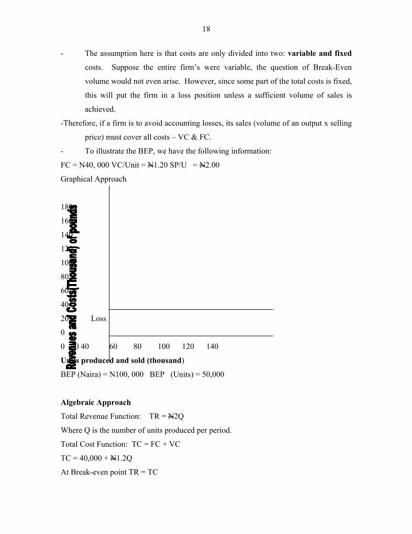
18
- The assumption here is that costs are only divided into two: variable and fixed
costs. Suppose the entire firm’s were variable, the question of Break-Even
volume would not even arise. However, since some part of the total costs is fixed,
this will put the firm in a loss position unless a sufficient volume of sales is
achieved.
-Therefore, if a firm is to avoid accounting losses, its sales (volume of an output x selling
price) must cover all costs – VC & FC.
- To illustrate the BEP, we have the following information:
FC = N40, 000 VC/Unit = N1.20 SP/U = N2.00
Graphical Approach
180
160
140
120
100
80
60
40
20 Loss
0
0 20 40 60 80 100 120 140
Units produced and sold (thousand)
BEP (Naira) = N100, 000 BEP (Units) = 50,000
Algebraic Approach
Total Revenue Function: TR = N2Q
Where Q is the number of units produced per period.
Total Cost Function: TC = FC + VC
TC = 40,000 + N1.2Q
At Break-even point TR = TC
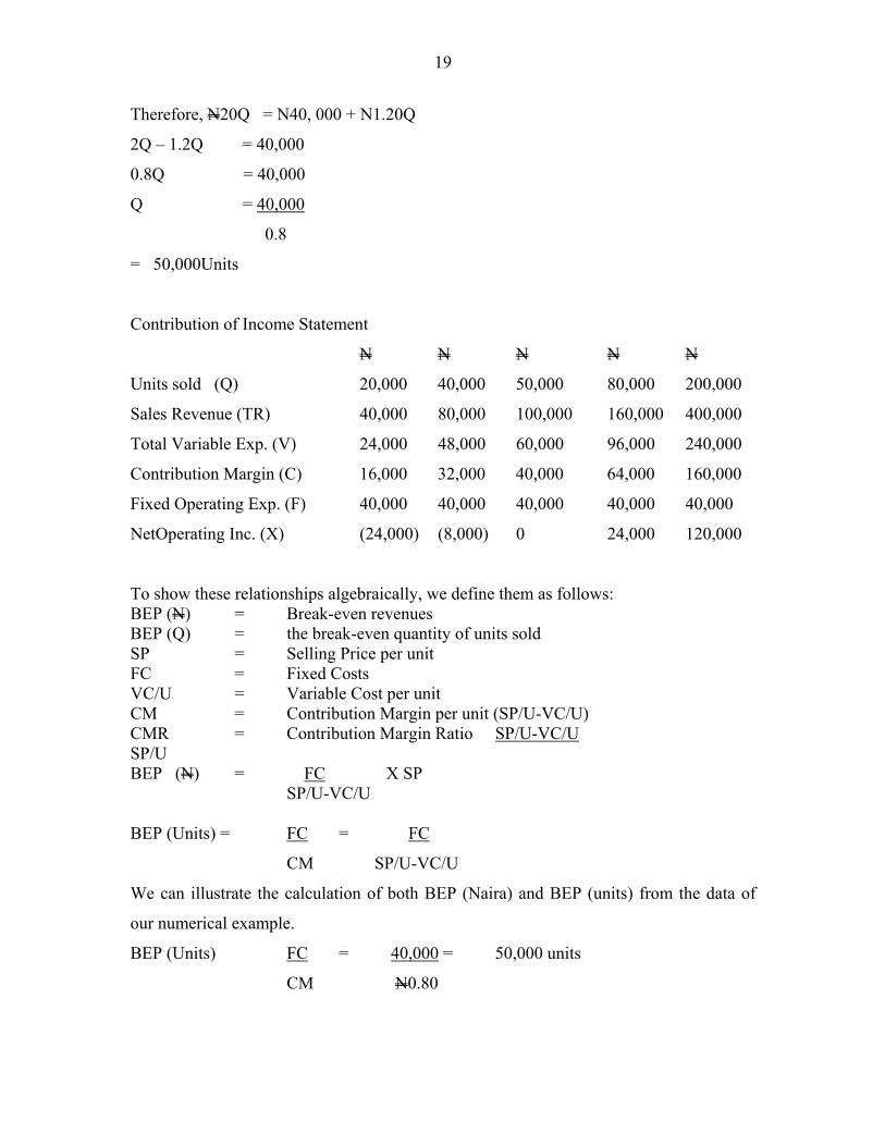
19
Therefore, N20Q = N40, 000 + N1.20Q
2Q – 1.2Q = 40,000
0.8Q = 40,000
Q = 40,000
0.8
= 50,000Units
Contribution of Income Statement
N N N N N
Units sold (Q) 20,000 40,000 50,000 80,000 200,000
Sales Revenue (TR) 40,000 80,000 100,000 160,000 400,000
Total Variable Exp. (V) 24,000 48,000 60,000 96,000 240,000
Contribution Margin (C) 16,000 32,000 40,000 64,000 160,000
Fixed Operating Exp. (F) 40,000 40,000 40,000 40,000 40,000
NetOperating Inc. (X) (24,000) (8,000) 0 24,000 120,000
To show these relationships algebraically, we define them as follows: BEP (N) = Break-even revenues BEP (Q) = the break-even quantity of units sold SP = Selling Price per unit FC = Fixed Costs VC/U = Variable Cost per unit CM = Contribution Margin per unit (SP/U-VC/U) CMR = Contribution Margin Ratio SP/U-VC/U SP/U BEP (N) = FC X SP
SP/U-VC/U BEP (Units) = FC = FC
CM SP/U-VC/U
We can illustrate the calculation of both BEP (Naira) and BEP (units) from the data of
our numerical example.
BEP (Units) FC = 40,000 = 50,000 units
CM N0.80
20
BEP (Naira) FC where:CMR=SP/U-VC/U =2-1.2 =0.4
SP/U 2
FC = 40,000 = N100, 000
CMR 0.4
Limitations of Simple BE Analysis
- Although it is useful in studying the relationships between costs, volume and
profits and it is a helpful in pricing, cost control and decision about expansion
programmes has its own limitations.
- Moreover, must of the limitations are centered around the unrealistic simplified
assumptions such as:-
(i) Constant Selling Price – Stability
(ii) Linearity of cost-volume-profit relationship
(iii) That there is no element of uncertainty
(iv) All cost can be divided into F & V.
FINANCIAL FORECASTING
Two major methods used in financial forecasting include:
(i) Percentage of sales method
(ii) Linear regression techniques especially simple regression technique.
- Simple regression model consists of the dependent variables and one independent
variable, which are assumed to be linearly related. The dependent variable is the
variable to be forecast, and the independent variable is an explanatory variable.
This model uses the least squares method to estimate the value of slope and
intercept.
Regression line = a + bX
Percentage of Sales Method
This method uses sales forecast as a base for forecasting financial requirements of the
firm.
- The assumption is that since a firm needs assets to make sales, then if sales are to
be increased, assets must also be increased. Increasing of assets of-course means
increasing finances.
- Further assumption is that the operation of the firm is 100% full capacity.
21
Illustration
The following balance sheet is for Dandima Development Company as December 2002
N N
Account Payable 50,000 Cash 10,000
Acc. Exp. 25,000 Debtors 85,000
Mortgage Bonds 70,000 Stock 100,000
Ordinary Share Capital 100,000 Net Fixed Assets 150,000
Retained Earnings 100,000
345,000 345,000
Additional Information:
The company’s sales are running at about N500, 000.00 a year at full capacity. The
profit margin after tax on sales is 4%. During 2002, the company earned N20, 000 after
taxes and paid out N10, 000 dividends; it plans to continue paying out half of net profits
as dividends. How much additional financing will be needed if sales expand to N800,
000 during 2003?
STEPS:
(i) Isolate the balance-sheet items that are likely to vary directly with sales.
(ii) Express these items as percentage of sales
(iii) Rewrite the balance sheet items in this percentage.
Pro forma Balance Sheet
N N
Account Payable 10.0 Cash 2.0
Acc. Exp. 5.0 Debtors 17.0
Mortgage Bonds NA Stock 20.0
Ordinary Share Capital NA Net Fixed Assets 30.0
Retained Earnings NA
15 69.0
Assets = .69
Less liabilities .15
.54
22
This means that for each N1.00 increase in sales, DDC must obtain N0.54 of financing either from internal or external or both. - Sales are to increase from 500,000 to 800,000 or by 300,000. To obtain the amount of financing required, we multiply 300,000 by N0.54 = N162, 000
- Internal Financing
Profit margin = 4%
Profit = 800,000 X 0.04 = N32, 000
- N (Dividend) 50% = N16, 000
- N32, 000 R. Earnings) = N16, 000
Total Financial Required = N162, 000
Less Amount raised internally = N16, 000
Amount to realised externally = N146, 000
OR
External funds needed = A (∆TR) - B (∆TR) – mb (TR2) TR TR
Where A = Assets that increase spontaneously with total revenue
TR
Where B = Assets that increase spontaneously with total revenue
TR
∆TR = Change in TR
m = Profit margin on sales
b = Earning retention ratio
TR2 = Total Revenue projected for the year
EFN = .69(300,000) - .15(300,000) – (.5) (.04) (800,000)
= 207,000 – 45,000 – 16,000
= N146, 000
Suppose sales forecast has been 3% increase or N515, 000
EFN = .69(15,000) – 0.15(15,000) – (0.5) (N515, 000)
= 10,350 – 2,250 – 10,300
= (N 2,200)
23
Under this circumstance, no external funds are required.
- The company has N 2,200 in excess of the requirements
- The company should therefore do any of the following or combination.
(i) Repay its debts
(ii) Increase dividends
(iii) Seek additional investment opportunities
We can also compute the percentage of the increase in sales that will have to be financed
externally (PEFR)
PEFR = i- m (1 + g) b g Where i = A - B
TR TR g = growth rate in sales
Using our earlier illustration:
i = 0.69 – 0.15 = 0.54
g = 300,000 + 500,000 = 60
PEFR = 0.54 - 0.04 (1.60)0.50
0.60
0.54 – 0.05333
= 48.6%
So 300,000 x 48.6%
PEFR = N146, 000
Suppose the inflation rate is considered and it is estimated at say 10 percent, we add this
to the previous 60 percent to obtain a growth rate of 70 percent.
At 70% PEFR = 0.54 - 0.04 (1.70)0.50
0.70
0.54 – 0.04857
= __ 0.49 or 49%
24
WORKING CAPITAL MANAGEMENT
This is the analysis that involves focusing on only part of the balance sheet by studying
current assets, current liabilities, and the relationship between these two sets of accounts.
The term working capital refers to the capital available for running the day to day
operations of an organization. It is defined as current assets less current liabilities.
Current assets include mainly cash, debtors and stock while current liabilities include
mainly creditors. Thus, working capital represents the firm’s investment in cash,
marketable security, account receivable, and inventories less the current liabilities used to
finance the current assets.
Concepts of Working Capital Management
In the discussion of working capital, it is good to distinguish between different concepts
of working capital.
Gross Working Capital - This refers to a firm’s investment in short-term assets – cash,
marketable securities, debtors, stock etc.
Net Working Capital- This is defined as current assets minus current liabilities used to
finance them such as short-term creditors and accrued expenses.
Working Capital Management – This refers to all aspects of the administration of both
current assets and current liabilities.
Importance of Working Capital Management
(i) Time devoted to Working Capital Management - Financial managers devote a lot
of time to the day-to-day internal operations of the firm’s working capital
management.
(ii) High Investment in Current Assets – Current Assets represent more than half the
total assets of a business firm and therefore worthy of the financial manager’s
careful attention.
(iii) Working Capital in Small Companies - It is particularly important to small firms
because they cannot avoid investment in cash, debtors and stock while they can
minimize investment in fixed (long term) assets by way of renting, hiring and
25
leasing (of plants and equipment for example). Therefore, serious attention must
be paid to working capital management.
(iv) Relationship between Sales Growth and Current Assets - There is close and direct
relationship between sales growth and the need to finance current assets. Consider
the cycle below:
Cash: Raw Materials W.I.P. Finished Goods
Debtors Sales
Determinants of Working Capital
There are no set rules or formulae for determining the working capital level a firm
should hold. It is however, determined by a wide range of factors. These include:
(i) General Nature of the Business – Example trading and financial firms have less
investment in fixed assets – only in working capital.
(ii) Promotion/Manufacturing Cycle - The longer the cycle, the longer the working
capital requirement.
(iii) Growth and Expansion – Growth industries require more working capital than
those that are static.
(iv) Dividend- Policy - The payment of dividend consumes cash resources, and
thereby affects working capital to that extent.
(v) Government Industrial Policy – For example, commercial banks are sometimes
required to maintain a certain minimum amount of cash in a special account with the
Central Bank, the lower the rate, the higher the working capital and vice-versa.
Other factors include business cycle, production policy, credit policy, profit level,
depreciation policy and so on.
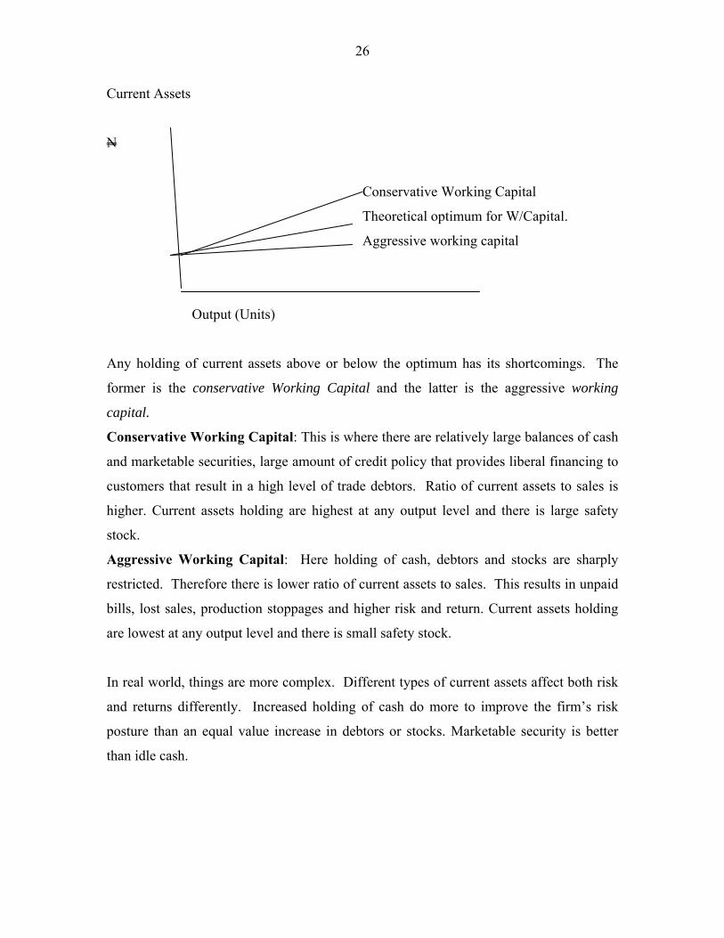
Optimum Level for Current Asset Investments
If a firm could be able to forecast perfectly enough cash to make disbursements as
required, enough stocks to meet production and sales requirements, the exact trade
debtors called for by an optimal credit policy and investment in marketable securities,
where the interest returns on such assets exceeded the cost of capital, it is referred to as
the theoretical optimum for working capital.
26
Current Assets
N
Conservative Working Capital
Theoretical optimum for W/Capital.
Aggressive working capital
Output (Units)
Any holding of current assets above or below the optimum has its shortcomings. The
former is the conservative Working Capital and the latter is the aggressive working
capital.
Conservative Working Capital: This is where there are relatively large balances of cash
and marketable securities, large amount of credit policy that provides liberal financing to
customers that result in a high level of trade debtors. Ratio of current assets to sales is
higher. Current assets holding are highest at any output level and there is large safety
stock.
Aggressive Working Capital: Here holding of cash, debtors and stocks are sharply
restricted. Therefore there is lower ratio of current assets to sales. This results in unpaid
bills, lost sales, production stoppages and higher risk and return. Current assets holding
are lowest at any output level and there is small safety stock.
In real world, things are more complex. Different types of current assets affect both risk
and returns differently. Increased holding of cash do more to improve the firm’s risk
posture than an equal value increase in debtors or stocks. Marketable security is better
than idle cash.
27
FINANCING CURRENT ASSETS
This is one of the important decisions involved in the general management of working
capital. There are three sources from which current assets may be financed. These
include long-term financing, short-term financing and spontaneous financing. Long term
financing source includes equity shares, debentures, retained- earnings. Short -term
financing refers to those sources of short-term credit that the firm must arrange in
advance and for which repayment would be due within one accounting period. Examples
are bank loans, commercial papers etc. Spontaneous financing refers to the automatic
sources of short-term funds usually required without formal negotiation. Examples are
trade creditors, bills payable accrued expenses as well as deferrals. They are usually
acquired at cost-free and so firms should utilize them to the fullest possible extent. This
area is not normally a difficult decision area as far as current assets financing is
concerned. Attention therefore is normally paid to short-term or long-term sources.
The three approaches to determining an appropriate financing mix are:
(i) Matching or hedging
(ii) Conservative
(iii) Aggressive
Matching (hedging) Approach refers to a process of matching of debt with the
maturities of financial needs. It further refers to the process of matching the expected life
of the assets purchased with the expected life of financing raised to pay for the assets.
Matching approach divides assets into two broad classes:
(i) Those that are required in a certain amount for a given level of operation, and, hence
do not vary over time; e.g. Fixed -assets and permanent current -assets.
(ii) Those which fluctuate over time (temporary current assets).
Set against the two assets classification are long-term and short-term financing sources
respectively.
28
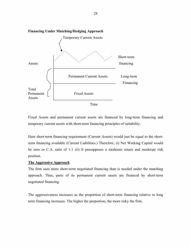
Financing Under Matching/Hedging Approach
Temporary Current Assets
Short-term
Assets financing
Permanent Current Assets Long-term
Financing
Total Permanent Fixed Assets Assets
Time
Fixed Assets and permanent current assets are financed by long-term financing and
temporary current assets with short-term financing principles of suitability.
Here short-term financing requirement (Current Assets) would just be equal to the short-
term financing available (Current Liabilities.) Therefore, (i) Net Working Capital would
be zero or C.A. ratio of 1:1 (ii) It presupposes a moderate return and moderate risk
position.
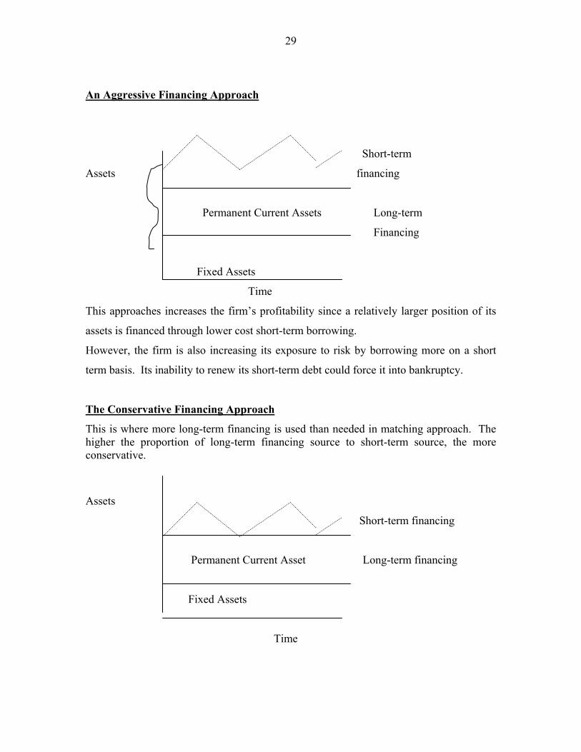
The Aggressive Approach
The firm uses more short-term negotiated financing than is needed under the matching
approach. Thus, parts of its permanent current assets are financed by short-term
negotiated financing.
The aggressiveness increases as the proportion of short-term financing relative to long
term financing increases. The higher the proportion, the more risky the firm.
29
An Aggressive Financing Approach
Short-term
Assets financing
Permanent Current Assets Long-term
Financing
Fixed Assets
Time
This approaches increases the firm’s profitability since a relatively larger position of its
assets is financed through lower cost short-term borrowing.
However, the firm is also increasing its exposure to risk by borrowing more on a short
term basis. Its inability to renew its short-term debt could force it into bankruptcy.
The Conservative Financing Approach
This is where more long-term financing is used than needed in matching approach. The higher the proportion of long-term financing source to short-term source, the more conservative.
Assets
Short-term financing
Permanent Current Asset Long-term financing
Fixed Assets
Time
30
Here the level of permanent financing is relatively higher than matching approach as
permanent funds are used to finance temporary fluctuating current assets. Thus, during
periods of low fluctuating current assets required by the firm may invest its excess funds
in marketable securities. The approach reduces the amount of funds requirements to be
borrowed temporary, resulting in high liquidity and so less risk of insolvency. However,
it suffers from low returns because;
(i) The cost of permanent financing is generally higher than the cost of short-term
credit.
(ii) Marketable securities have a relatively low rate of return compared to the returns
from on going long-term projects.
Which Approach to Adopt?
It is not an easy task for a financial manager to decide on one of the three approaches to
adopt. Where all the variables the approaches assumed to be known one in practice,
really knows the task then becomes easy one. Since the world of practice is however full
of uncertainties, most financial managers use estimates by way of attaching certain
probabilities to the occurrence levels of each variable to easy their decisions. They then
determine the risk to take and the appropriate return acceptable to the risk taken. This is
so because, as already shown, whatever approach is taken, there are risks as well as
returns considerations. Financial managers are then in a risk-return tangle.
TC Function
Cost of Liquidity
Cost of Illiquidity
Optimum Level
COMPONENTS OF WORKING CAPITAL
The components of working capital are cash, marketable securities, debtors and stock
(inventory).
31
A. Cash & Marketable Securities Management
This involves managing the monies of the firm in order to attain maximum cash available
and maximum interest income on any idle fund. It is also concerned with the most
effective ways of accelerating collections and handling cash disbursements so that
maximum cash is available.
Motives for Holding Cash
(i) Transaction motive
(ii) Precautionary motive
(iii) Speculative motive
(iv) Compensation- balance – motive
Transaction motive: A firm needs to hold cash in ordinary course of business for the day–
to–day operations. For instance, cash is needed to pay creditors, t buy stocks, to pay
wages, operating expenses, taxes, dividends etc.
Precautionary motive: A firm needs too hold cash to meet any contingencies in the
future. Contingent losses may be material; .e.g. pending law suits against the company or
a bill of exchange that that the company has accepted. Holding cash provides a cushion to
withstand unexpected emergency cash flows.
Speculative motive: A firm needs to hold cash to finance profitable investment
opportunities as and when they arise. The investment opportunities might be risky
ventures, e.g. purchasing a machine for a speculative project.
Compensating Balance Motive: Banks typically require that a regular borrower maintains
an average account balance equal to 15% to 20% of the outstanding loan. This balance,
commonly called Compensating balance, is a method of raising the effective interest rate.
32
Cash Management Models
Several types of mathematical models have been developed to help determine optimal
cash balances. An early model developed by William J. Baumol applies a basic
inventory model to cash management. The model believes that there are costs for too low
or too high cash balance. It is assumed that a firm on the average is growing and is a net
user of cash. Marketable securities in the model represent a buffer stock between
episodes of external financing, which is drawn down as required periodically. Ordering
costs are represented by the clerical and transactions costs of making transfer between the
investment portfolio and the cash account. The holding cost is the interest foregone on
cash balances held. It is also assumed that cash expenditure occurs evenly over-time and
that cash replenishment comes in lump sum at periodic interval.
Baumol formulated the optimal size of cash transfer as follows:
c= 2bt Where: i
c = Optimal cash transaction
t = Total cash usage for the period of time involved b = Cost of the transaction in the purchase or sale of marketable securities i = the applicable interest rate on marketable securities Illustration
A company’s total demand for cash for one year is N1, 800,000. The cost of transaction
is N25. Applicable interest on marketable securities is 10%. Compute the firm’s optimum
size of cash transaction.
Solution:
t = 1.8m b = N25, i = 10%
c = √2bt = √ 2(25) (1,800,000) = N30, 000 i 0.1 Average cash balance - C/2 = 30,000/2= N15, 000 No. of transfer/operations per year t⁄c = 1,800,000 = 60 times 5 times /month Total cost of maintaining cash balance per year TC b (T/C) + i (C/2) 25 (1.8m) + .1 (30,000) 30,000 2
TC = N3, 000
33
Illustration Two
Firm XYZ estimates cash payment of N6, 000,000 for one-month period and the payment
is expected to be steady over the period. The fixed amount of transaction is N100.
Interest rate on marketable securities = 15% annum (or 1.25/month) Determine:
(a) The optimum size of its cash transactions
(b) Average cash balance
(c) Number of transfer/operations
(d) Total cost of maintaining cash balance per month.
C =√2bt /i t = 6m b=N100
i = 15%/year or 1.25/month
(a) C = √2(100) (6,000,000) = N309, 839 0.0125 (b) C/2 = 309,839 ⁄2 = 154,919.50 Average cash usage (c) t/c = 6,000,000 = 19.36 per month 309,839 (d) = b (t/c) + i(c/2) = 100(6,000,000) +0.0125(309,839) 309,839 2 1936 + 1936.49 =3872.49 MILLER-ORR MODEL
Miller and Orr expanded the Baumol model by incorporating a stochastic generating
process for periodic changes in cash balances. It is applied in situations where there is
uncertainty of cash payment since EOQ cash model may not be applicable if cash-
balances fluctuate randomly.
Thus the only control limits is to set up lower and higher limit of tolerance. If cash
demand is stochastic and unknown in advance, transfers from cash to marketable
securities is required if cash balances reach the upper limit. On the other hand, when it
reaches the lower limit, the transfer from marketable securities to cash is triggered.
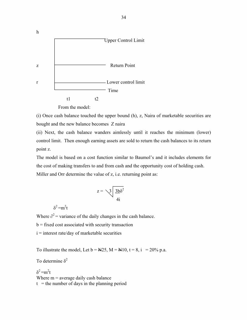
34
h
Upper Control Limit
z Return Point
r Lower control limit
Time
t1 t2
From the model:
(i) Once cash balance touched the upper bound (h), z, Naira of marketable securities are
bought and the new balance becomes Z naira
(ii) Next, the cash balance wanders aimlessly until it reaches the minimum (lower)
control limit. Then enough earning assets are sold to return the cash balances to its return
point z.
The model is based on a cost function similar to Baumol’s and it includes elements for
the cost of making transfers to and from cash and the opportunity cost of holding cash.
Miller and Orr determine the value of z, i.e. returning point as: z = 3 3b2
4i
2 =m2t
Where ∂2 = variance of the daily changes in the cash balance.
b = fixed cost associated with security transaction
i = interest rate/day of marketable securities
To illustrate the model, Let b = N25, M = N10, t = 8, i = 20% p.a. To determine 2 2 =m2t Where m = average daily cash balance t = the number of days in the planning period
35
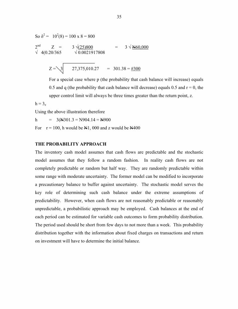
So 2 = 102(8) = 100 x 8 = 800 2nd Z = 3 √(25)800 = 3 √ N60,000 √ 4(0.20/365 √ 0.0021917808 Z = 3 27,375,010.27 = 301.38 = #300
For a special case where p (the probability that cash balance will increase) equals
0.5 and q (the probability that cash balance will decrease) equals 0.5 and r = 0, the
upper control limit will always be three times greater than the return point, z.
h = 3z
Using the above illustration therefore
h = 3(N301.3 = N904.14 = N900
For r = 100, h would be N1, 000 and z would be N400
THE PROBABILITY APPROACH
The inventory cash model assumes that cash flows are predictable and the stochastic
model assumes that they follow a random fashion. In reality cash flows are not
completely predictable or random but half way. They are randomly predictable within
some range with moderate uncertainty. The former model can be modified to incorporate
a precautionary balance to buffer against uncertainty. The stochastic model serves the
key role of determining such cash balance under the extreme assumptions of
predictability. However, when cash flows are not reasonably predictable or reasonably
unpredictable, a probabilistic approach may be employed. Cash balances at the end of
each period can be estimated for variable cash outcomes to form probability distribution.
The period used should be short from few days to not more than a week. This probability
distribution together with the information about fixed charges on transactions and return
on investment will have to determine the initial balance.
36
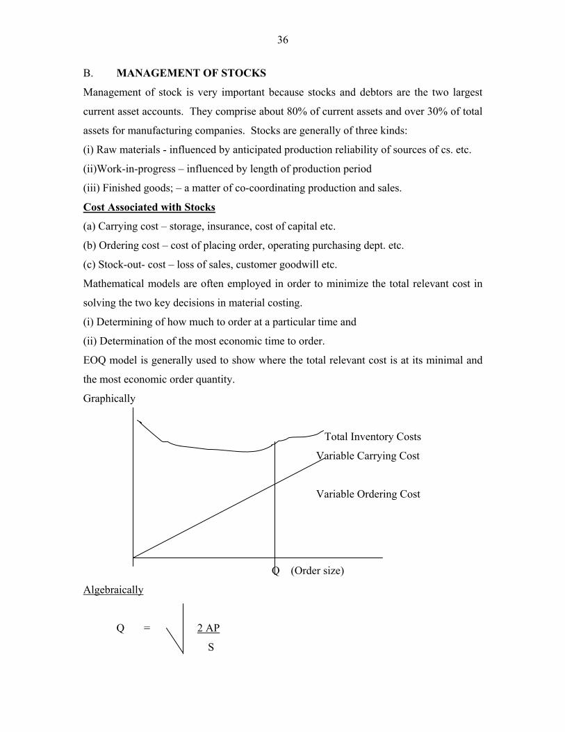
B. MANAGEMENT OF STOCKS
Management of stock is very important because stocks and debtors are the two largest
current asset accounts. They comprise about 80% of current assets and over 30% of total
assets for manufacturing companies. Stocks are generally of three kinds:
(i) Raw materials - influenced by anticipated production reliability of sources of cs. etc.
(ii)Work-in-progress – influenced by length of production period
(iii) Finished goods; – a matter of co-coordinating production and sales.
Cost Associated with Stocks
(a) Carrying cost – storage, insurance, cost of capital etc.
(b) Ordering cost – cost of placing order, operating purchasing dept. etc.
(c) Stock-out- cost – loss of sales, customer goodwill etc.
Mathematical models are often employed in order to minimize the total relevant cost in
solving the two key decisions in material costing.
(i) Determining of how much to order at a particular time and
(ii) Determination of the most economic time to order.
EOQ model is generally used to show where the total relevant cost is at its minimal and
the most economic order quantity.
Graphically
Total Inventory Costs
Variable Carrying Cost
Variable Ordering Cost
Q (Order size)
Algebraically
Q = 2 AP
S
37
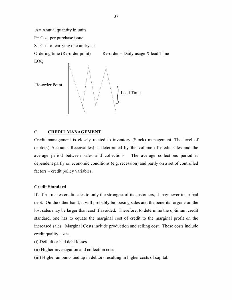
A= Annual quantity in units
P= Cost per purchase issue
S= Cost of carrying one unit/year
Ordering time (Re-order point) Re-order = Daily usage X lead Time
EOQ
Re-order Point
Lead Time
C. CREDIT MANAGEMENT
Credit management is closely related to inventory (Stock) management. The level of
debtors( Accounts Receivables) is determined by the volume of credit sales and the
average period between sales and collections. The average collections period is
dependent partly on economic conditions (e.g. recession) and partly on a set of controlled
factors – credit policy variables.
Credit Standard
If a firm makes credit sales to only the strongest of its customers, it may never incur bad
debt. On the other hand, it will probably be loosing sales and the benefits forgone on the
lost sales may be larger than cost if avoided. Therefore, to determine the optimum credit
standard, one has to equate the marginal cost of credit to the marginal profit on the
increased sales. Marginal Costs include production and selling cost. These costs include
credit quality costs.
(i) Default or bad debt losses
(ii) Higher investigation and collection costs
(iii) Higher amounts tied up in debtors resulting in higher costs of capital.
38
Since credit cost and credit quality are negatively correlated, it is important to be able to
judge the quality of a customer, and perhaps the best way to do this is in terms of the
probability of default. A good credit manager should therefore be able to make a near
accurate judgment of his customers. In evaluating any credit policy, the benefits of the
policy should be compared with the costs of the policy. For instance, the benefits of a
proposed policy to ease credit terms include increases in sales and profit from sales,
while the costs of the policy include:
(i) Interest charges on an additional increase in debtors.
(ii) Increase in bad debt.
FIVE Cs of CREDIT
To evaluate the credit-risk, credit managers should consider the five Cs of credit:
Character of the Customer: This is subjective – willingness to pay. Some
customers are capable but not willing to pay N 100,000 in debit collection, and
average collection period of 2 months. Bad debt also currently amounts to
Capacity: The customer’s ability to pay. Look at past Behaviour of the
customers and making physical investigation of the customers’ assets like store,
balance sheet records etc.
Capital: A measure of the general financial situation of the firm’s position with
special attention to risk ratios and time interest analysis ratio.
Collateral: Security – what a customer places against the loan.
Conditions: The general economic conditions. Is it boom or doom condition?
These represent the factors by which the credit risks are judged.
Terms of Credit
These specify the period for which credit is extended and the discount if any, for early
payment. E.g. if a firm’s credit terms to all approved customers are stated as 2/10, net 30,
then 2% discount from the stated sales price is granted if payment is made within 10
days, and the entire amount is due 10 days from the invoice date if the discount is not
taken. If the terms are stated ‘net 60’, this indicates that no discount is offered and that
the bill is due and payable 60 days after the invoice date.
39
Credit Period
Lengthening the credit period is likely to stimulate sales, but there is a cost to tying up
funds in debtors. For example, if a firm changes its terms from net 30 to net 60, the
average debtors for the year may rise from N100,000 to N300,000 – the increase is
caused partly by the longer credit terms and partly by the larger volume of sales. The
optimal credit policy is therefore determined by the point where marginal profits on
increased sales are exactly offset by the cost carrying the higher amount of debtors.
Practice Question
Dotcom Ltd. With a turnover of N3 million is currently contemplating changing its debt
collection policy. It currently incurs administrative cost of N 100,000 in debt collection
and average collection is 2 months. Bad debt also currently amounts to 2.5% of sales.
The company is considering two options as follows:
Option A Option B
Administrative cost of bad debt #150,000 #10,000
Bad debt losses (% of sales) 1.5% -
Average collection period 1 month 1/5
Factoring fee (% of sales) - 3%
The company currently requires a 16% return on its investment. Please advice the
company on the best option.
40
CAPITAL BUDGETING
(a) Introduction
This involves the entire process of planning expenditure whose returns are expected to
extend beyond one year. Capital expenditure which is expected to yield benefit in two
or more years include expenditure for land, building, machinery, advertising and sales
promotions etc. The decision to invest in these areas based on cost-benefit analysis is
called capital budgeting decision.
(b) Features of Capital Budgeting:
Investment decisions are generally grouped into three:
The problems of searching out project and obtaining information about them.
Deciding which project(s) to invest and the extent of investment in each and;
Deciding upon the sources of finance upon which to draw and how much to
obtain from each source.
The third of these decisions is the principal concern of Capital Budgeting. There are
three capital budgeting decisions:
(a) The accept-reject decisions
(b) Mutually exclusive choice decisions
(c) Capital rationing decisions
(c) Cash Flow Analysis
After the firm has decided to embark on any capital expenditure, estimates of cash
inflows and outflows in respect of each respective proposal must be determined.
However, it is difficult to predict the outcome of an investment with certainty in
determining;
(a) The net cash inflows for each proposal, one must consider the cost of the new project,
the installation costs (if any i.e. income taxes etc.)
(b)The net cash inflows on the other hand, all expected benefits from a proposed project
must be measured on a cash flow basis, profit after taxes and depreciation
41
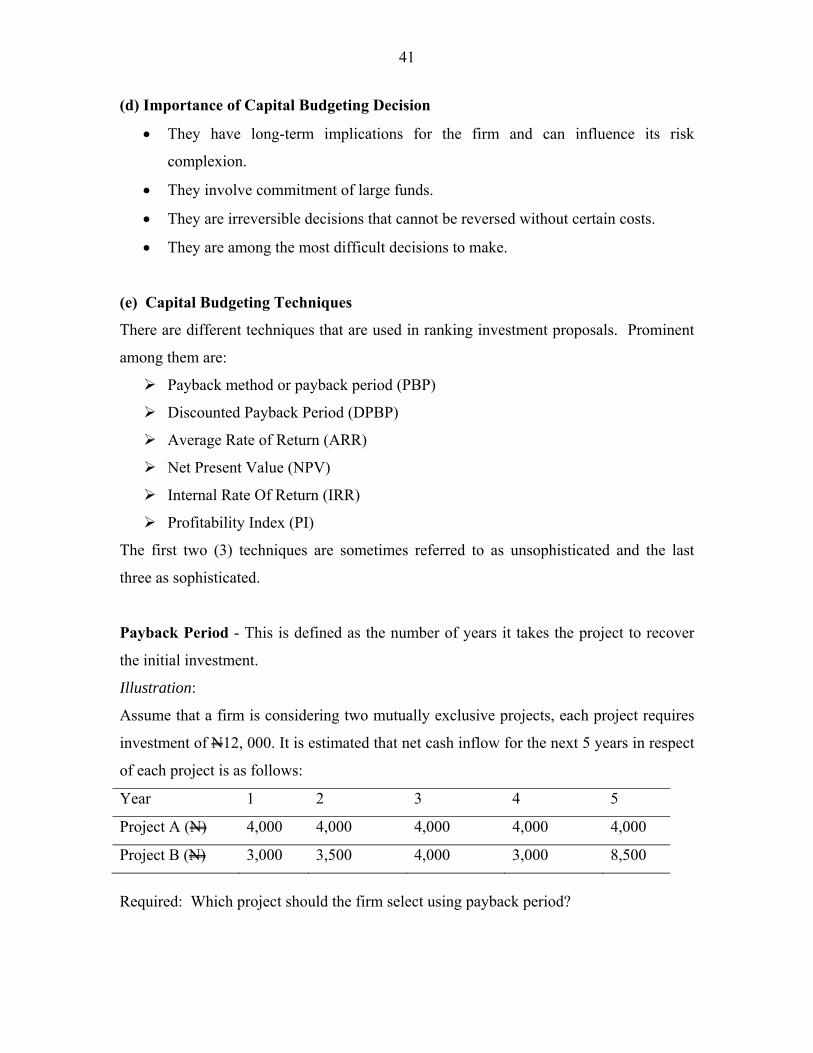
(d) Importance of Capital Budgeting Decision
They have long-term implications for the firm and can influence its risk
complexion.
They involve commitment of large funds.
They are irreversible decisions that cannot be reversed without certain costs.
They are among the most difficult decisions to make.
(e) Capital Budgeting Techniques
There are different techniques that are used in ranking investment proposals. Prominent
among them are:
Payback method or payback period (PBP)
Discounted Payback Period (DPBP)
Average Rate of Return (ARR)
Net Present Value (NPV)
Internal Rate Of Return (IRR)
Profitability Index (PI)
The first two (3) techniques are sometimes referred to as unsophisticated and the last
three as sophisticated.
Payback Period - This is defined as the number of years it takes the project to recover
the initial investment.
Illustration:
Assume that a firm is considering two mutually exclusive projects, each project requires
investment of N12, 000. It is estimated that net cash inflow for the next 5 years in respect
of each project is as follows:
Year 1 2 3 4 5
Project A (N) 4,000 4,000 4,000 4,000 4,000
Project B (N) 3,000 3,500 4,000 3,000 8,500
Required: Which project should the firm select using payback period?
42
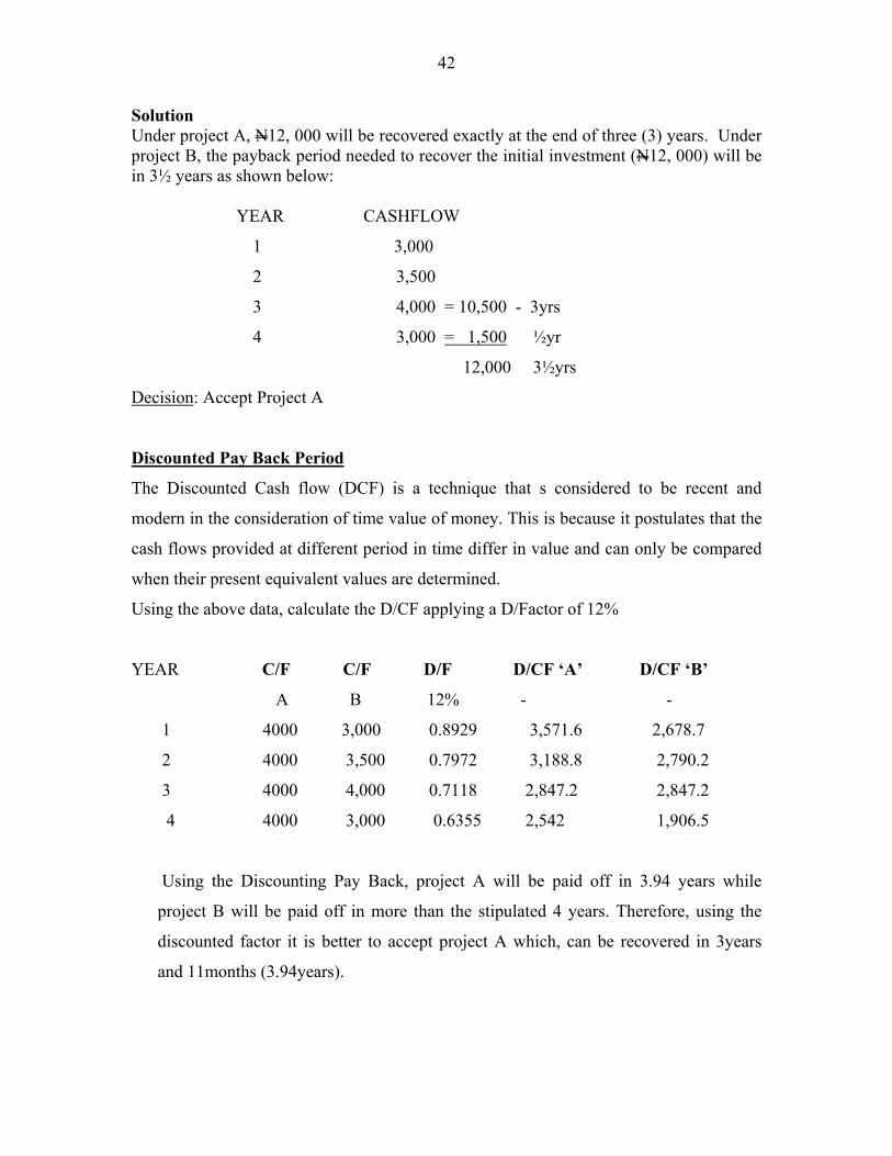
Solution Under project A, N12, 000 will be recovered exactly at the end of three (3) years. Under project B, the payback period needed to recover the initial investment (N12, 000) will be in 3½ years as shown below:
YEAR CASHFLOW
1 3,000
2 3,500
3 4,000 = 10,500 - 3yrs
4 3,000 = 1,500 ½yr
12,000 3½yrs
Decision: Accept Project A
Discounted Pay Back Period
The Discounted Cash flow (DCF) is a technique that s considered to be recent and
modern in the consideration of time value of money. This is because it postulates that the
cash flows provided at different period in time differ in value and can only be compared
when their present equivalent values are determined.
Using the above data, calculate the D/CF applying a D/Factor of 12%
YEAR C/F C/F D/F D/CF ‘A’ D/CF ‘B’
A B 12% - -
1 4000 3,000 0.8929 3,571.6 2,678.7
2 4000 3,500 0.7972 3,188.8 2,790.2
3 4000 4,000 0.7118 2,847.2 2,847.2
4 4000 3,000 0.6355 2,542 1,906.5
Using the Discounting Pay Back, project A will be paid off in 3.94 years while
project B will be paid off in more than the stipulated 4 years. Therefore, using the
discounted factor it is better to accept project A which, can be recovered in 3years
and 11months (3.94years).
43
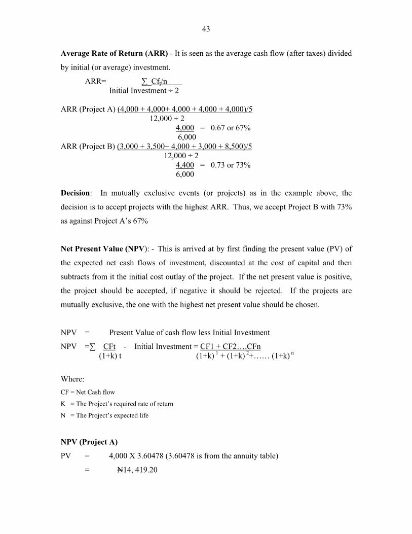
Average Rate of Return (ARR) - It is seen as the average cash flow (after taxes) divided
by initial (or average) investment.
ARR= ∑_Cft/n Initial Investment ÷ 2
ARR (Project A) (4,000 + 4,000+ 4,000 + 4,000 + 4,000)/5 12,000 ÷ 2
4,000 = 0.67 or 67% 6,000
ARR (Project B) (3,000 + 3,500+ 4,000 + 3,000 + 8,500)/5 12,000 ÷ 2 4,400 = 0.73 or 73% 6,000 Decision: In mutually exclusive events (or projects) as in the example above, the
decision is to accept projects with the highest ARR. Thus, we accept Project B with 73%
as against Project A’s 67%
Net Present Value (NPV): - This is arrived at by first finding the present value (PV) of
the expected net cash flows of investment, discounted at the cost of capital and then
subtracts from it the initial cost outlay of the project. If the net present value is positive,
the project should be accepted, if negative it should be rejected. If the projects are
mutually exclusive, the one with the highest net present value should be chosen.
NPV = Present Value of cash flow less Initial Investment
NPV =∑ CFt - Initial Investment = CF1 + CF2….CFn (1+k) t (1+k) 1 + (1+k) 2+…… (1+k) n
Where:
CF = Net Cash flow
K = The Project’s required rate of return
N = The Project’s expected life
NPV (Project A)
PV = 4,000 X 3.60478 (3.60478 is from the annuity table)
= N14, 419.20
44
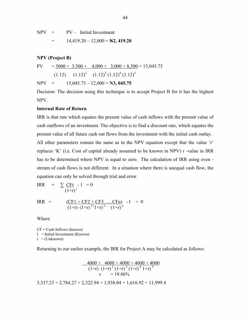
NPV = PV – Initial Investment
= 14,419.20 – 12,000 = N2, 419.20
NPV (Project B)
PV = 3000 + 3,500 + 4,000 + 3,000 + 8,500 = 15,045.75
(1.12) (1.12)2 (1.12)3 (1.12)4 (1.12)5
NPV = 15,045.75 – 12,000 = N3, 045.75
Decision: The decision using this technique is to accept Project B for it has the highest
NPV.
Internal Rate of Return
IRR is that rate which equates the present value of cash inflows with the present value of
cash outflows of an investment. The objective is to find a discount rate, which equates the
present value of all future cash out flows from the investment with the initial cash outlay.
All other parameters remain the same as in the NPV equation except that the value ‘r’
replaces ‘K’ (i.e. Cost of capital already assumed to be known in NPV) r -value in IRR
has to be determined where NPV is equal to zero. The calculation of IRR using even -
stream of cash flows is not different. In a situation where there is unequal cash flow, the
equation can only be solved through trial and error.
IRR = ∑ CFt - 1 = 0 (1+r) t
IRR = (CF1 + CF2 + CF3 …..CFn) - I = 0 (1+r) (1+r) 2 (1+r) 3….. (1+r) n Where CF = Cash Inflows (known) I = Initial Investment (Known) r = (Unknown) Returning to our earlier example, the IRR for Project A may be calculated as follows:
4000 + 4000 + 4000 + 4000 + 4000 (1+r) (1+r) 2 (1+r) 3 (1+r) 4 1+r) 5 r = 19.86%
3,337.23 + 2,784.27 + 2,322.94 + 1,938.04 + 1,616.92 = 11,999.4
45
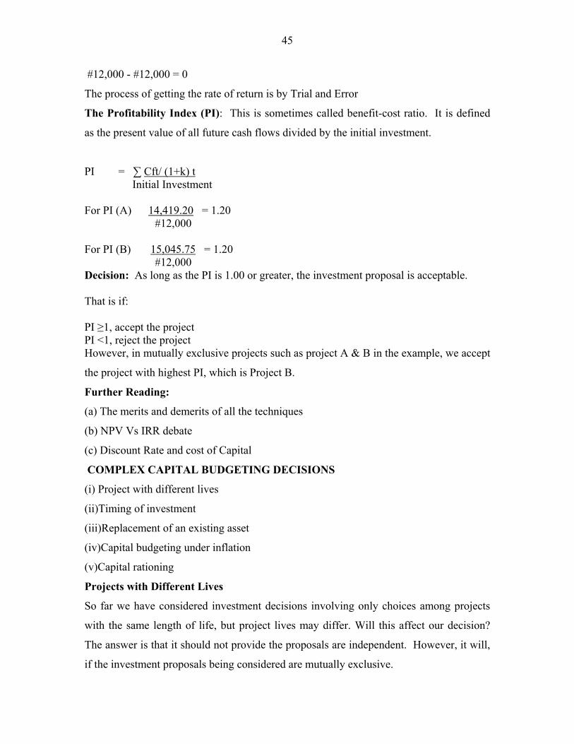
#12,000 - #12,000 = 0
The process of getting the rate of return is by Trial and Error
The Profitability Index (PI): This is sometimes called benefit-cost ratio. It is defined
as the present value of all future cash flows divided by the initial investment.
PI = ∑ Cft/ (1+k) t Initial Investment For PI (A) 14,419.20 = 1.20 #12,000 For PI (B) 15,045.75 = 1.20 #12,000 Decision: As long as the PI is 1.00 or greater, the investment proposal is acceptable. That is if: PI ≥1, accept the project PI <1, reject the project However, in mutually exclusive projects such as project A & B in the example, we accept
the project with highest PI, which is Project B.
Further Reading:
(a) The merits and demerits of all the techniques
(b) NPV Vs IRR debate
(c) Discount Rate and cost of Capital
COMPLEX CAPITAL BUDGETING DECISIONS
(i) Project with different lives
(ii)Timing of investment
(iii)Replacement of an existing asset
(iv)Capital budgeting under inflation
(v)Capital rationing
Projects with Different Lives
So far we have considered investment decisions involving only choices among projects
with the same length of life, but project lives may differ. Will this affect our decision?
The answer is that it should not provide the proposals are independent. However, it will,
if the investment proposals being considered are mutually exclusive.
46
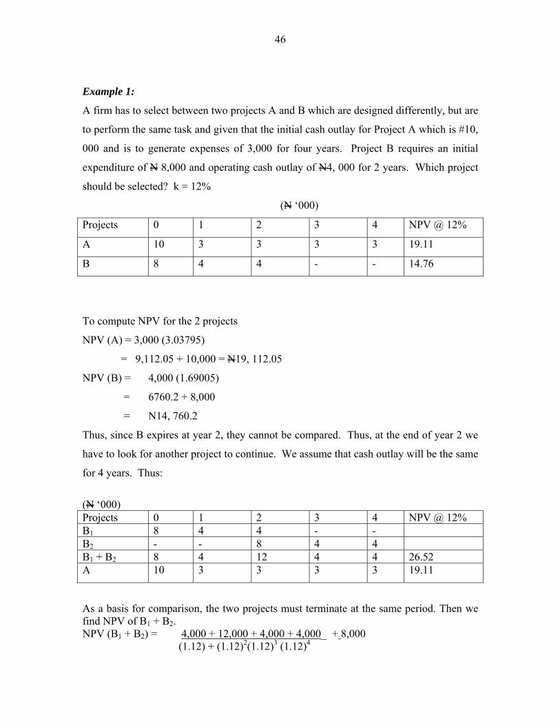
Example 1:
A firm has to select between two projects A and B which are designed differently, but are
to perform the same task and given that the initial cash outlay for Project A which is #10,
000 and is to generate expenses of 3,000 for four years. Project B requires an initial
expenditure of N 8,000 and operating cash outlay of N4, 000 for 2 years. Which project
should be selected? k = 12%
(N ‘000)
Projects 0 1 2 3 4 NPV @ 12%
A 10 3 3 3 3 19.11
B 8 4 4 - - 14.76
To compute NPV for the 2 projects
NPV (A) = 3,000 (3.03795)
= 9,112.05 + 10,000 = N19, 112.05
NPV (B) = 4,000 (1.69005)
= 6760.2 + 8,000
= N14, 760.2
Thus, since B expires at year 2, they cannot be compared. Thus, at the end of year 2 we
have to look for another project to continue. We assume that cash outlay will be the same
for 4 years. Thus:
(N ‘000) Projects 0 1 2 3 4 NPV @ 12% B1 8 4 4 - - B2 - - 8 4 4 B1 + B2 8 4 12 4 4 26.52 A 10 3 3 3 3 19.11
As a basis for comparison, the two projects must terminate at the same period. Then we find NPV of B1 + B2. NPV (B1 + B2) = 4,000 + 12,000 + 4,000 + 4,000_ + 8,000 (1.12) + (1.12)2(1.12)3 (1.12)4
47
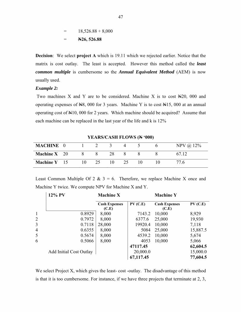
= 18,526.88 + 8,000
= N26, 526.88
Decision: We select project A which is 19.11 which we rejected earlier. Notice that the
matrix is cost outlay. The least is accepted. However this method called the least
common multiple is cumbersome so the Annual Equivalent Method (AEM) is now
usually used.
Example 2:
Two machines X and Y are to be considered. Machine X is to cost N20, 000 and
operating expenses of N8, 000 for 3 years. Machine Y is to cost N15, 000 at an annual
operating cost of N10, 000 for 2 years. Which machine should be acquired? Assume that
each machine can be replaced in the last year of the life and k is 12%
YEARS/CASH FLOWS (N ‘000)
MACHINE 0 1 2 3 4 5 6 NPV @ 12%
Machine X 20 8 8 28 8 8 8 67.12
Machine Y 15 10 25 10 25 10 10 77.6
Least Common Multiple Of 2 & 3 = 6. Therefore, we replace Machine X once and
Machine Y twice. We compute NPV for Machine X and Y.
12% PV Machine X Machine Y
Cash Expenses (C.E)
PV (C.E) Cash Expenses (C.E)
PV (C.E)
1 0.8929 8,000 7143.2 10,000 8,929 2 0.7972 8,000 6377.6 25,000 19,930 3 0.7118 28,000 19920.4 10,000 7,118 4 0.6355 8,000 5084 25,000 15,887.5 5 0.5674 8,000 4539.2 10,000 5,674 6 0.5066 8,000 4053 10,000 5,066 47117.45 62,604.5 Add Initial Cost Outlay 20,000.0 15,000.0 67,117.45 77,604.5
We select Project X, which gives the least- cost -outlay. The disadvantage of this method
is that it is too cumbersome. For instance, if we have three projects that terminate at 2, 3,
48
and 5 years, the least common multiple will be 30 years. Therefore, the Annual
Equivalent Method is more preferred.
Example 3:
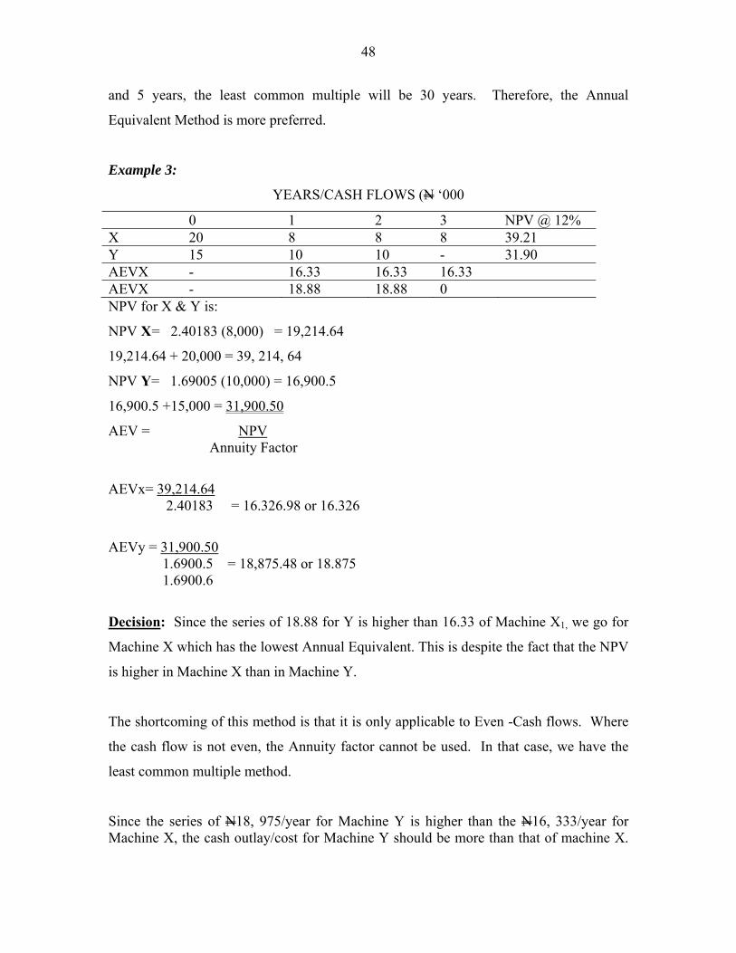
YEARS/CASH FLOWS (N ‘000
0 1 2 3 NPV @ 12% X 20 8 8 8 39.21 Y 15 10 10 - 31.90 AEVX - 16.33 16.33 16.33 AEVX - 18.88 18.88 0 NPV for X & Y is:
NPV X = 2.40183 (8,000) = 19,214.64
19,214.64 + 20,000 = 39, 214, 64
NPV Y= 1.69005 (10,000) = 16,900.5
16,900.5 +15,000 = 31,900.50
AEV = NPV Annuity Factor
AEVx= 39,214.64 2.40183 = 16.326.98 or 16.326
AEVy = 31,900.50 1.6900.5 = 18,875.48 or 18.875 1.6900.6
Decision: Since the series of 18.88 for Y is higher than 16.33 of Machine X1, we go for
Machine X which has the lowest Annual Equivalent. This is despite the fact that the NPV
is higher in Machine X than in Machine Y.
The shortcoming of this method is that it is only applicable to Even -Cash flows. Where
the cash flow is not even, the Annuity factor cannot be used. In that case, we have the
least common multiple method.
Since the series of N18, 975/year for Machine Y is higher than the N16, 333/year for Machine X, the cash outlay/cost for Machine Y should be more than that of machine X.
49
If machine X and Y were assumed to be replaced indefinitely, then the NPV cost of Machine X and Y in perpetuating would be: Machine X = 16,327 = N136, 058 0.12 Machine Y = 18,875 = N157, 292
0.12 Difference = N21, 233. The company will therefore be better up by 21,233 by always investing in machine X.
Practice Question: The management of a company has decided to purchase a copier for
its purchasing Dept...The alternative has been broken down to two models. Model X
costing N15, 000 and Model Y costing N8, 000. The net cash benefits from Y are
estimated at N5, 000 a year to 5 years whereas the benefits from Y are estimated @ N4,
500 a year to three years. Management has decided not to count the salvage value for
either model, because of the high obsolescence rate for such equipment. The required rate
of return for a new copier has been at 10%, which model should be purchased.
INVESTMENT TIMING
A firm evaluates a number of investment projects every year. In the absence of capital
constraints all projects with positive NPVs are acceptable and vice-versa. Again some
projects may be more profitable i.e. higher positive value than others if undertaking in
future than now. It is also possible that some unprofitable projects i.e. those with negative
NPV may be profitable if considered later. These last categories may have different
degrees of postponement – 1, 2, 3 years etc. The firm should therefore determine the
optimum time of investment.
How do we then determine the optimum timing of an investment project? The rule
should be to undertake the project at that point of time, which maximizes the NPV.
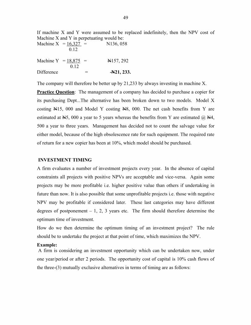
Example: A firm is considering an investment opportunity which can be undertaken now, under
one year/period or after 2 periods. The opportunity cost of capital is 10% cash flows of
the three-(3) mutually exclusive alternatives in terms of timing are as follows:
50
‘000
PERIODS 0 1 2 3 0 -100 150 1 -120 180 2 -140 205
When should the firm undertake this project? First, calculate NPV of each project.
‘000
0 1 2 3 NPV 0-100 150 x 0.9091
= N136.37 N36.37
1 - -120x0.9091 = N-109.09
180x.82645 =N 148.76
N39.67
2 -140 x0.82645
=N -115.70
205x0.7513
=N154.02
N38.32
Decision: We select the situation where the NPV is highest i.e. N39.67
REPLACING AN EXISTING ASSET
Investments are often made to replace existing assets, which are worn-out or less efficient
than new machine. Management must therefore decide when to replace existing assets
that decision must be based on economic consideration.
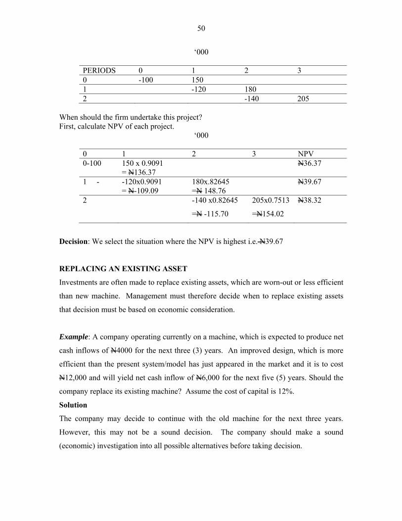
Example: A company operating currently on a machine, which is expected to produce net
cash inflows of N4000 for the next three (3) years. An improved design, which is more
efficient than the present system/model has just appeared in the market and it is to cost
N12,000 and will yield net cash inflow of N6,000 for the next five (5) years. Should the
company replace its existing machine? Assume the cost of capital is 12%.
Solution
The company may decide to continue with the old machine for the next three years.
However, this may not be a sound decision. The company should make a sound
(economic) investigation into all possible alternatives before taking decision.
51
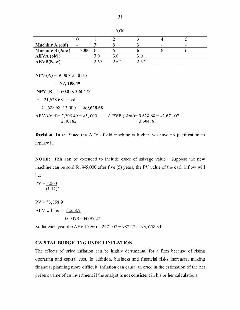
‘000
0 1 2 3 4 5 Machine A (old) - 3 3 3 - - Machine B (New) -12000 6 6 6 6 6 AEVA (old ) 3.0 3.0 3.0 AEVB(New) 2.67 2.67 2.67
NPV (A) = 3000 x 2.40183
= N7, 205.49
NPV (B) = 6000 x 3.60478
= 21,628.68 – cost
=21,628.68–12,000 = N9,628.68
AEVA(old)= 7,205.49 = #3, 000 A EVB (New)= 9,628.68 = #2,671.07 2.40182 3.60478
Decision Rule: Since the AEV of old machine is higher, we have no justification to
replace it.
NOTE: This can be extended to include cases of salvage value. Suppose the new
machine can be sold for N5,000 after five (5) years, the PV value of the cash inflow will
be:
PV = 5,000 (1.12)5
PV = #3,558.9
AEV will be: 3,558.9
3.60478 = N987.27
So far each year the AEV (New) = 2671.07 + 987.27 = N3, 658.34
CAPITAL BUDGETING UNDER INFLATION
The effects of price inflation can be highly detrimental for a firm because of rising
operating and capital cost. In addition, business and financial risks increases, making
financial planning more difficult. Inflation can cause an error in the estimation of the net
present value of an investment if the analyst is not consistent in his or her calculations.
52
Consistency requires that both the required rate of return and estimated cash flows of the
investment be stated in either “normal” terms or “real” terms. If the former are used, the
required rate of return will be based on current financing rates, which will include an
inflation component determined in the market. The required rate of return in this case is
not adjusted by the analyst to eliminate the effect of inflation cash flow also.
On the other hand, if real terms are used, both the required rate of return and the future
cash flows will have to be inflation- adjusted i.e. they will have to be reduced to eliminate
the effect of inflation.
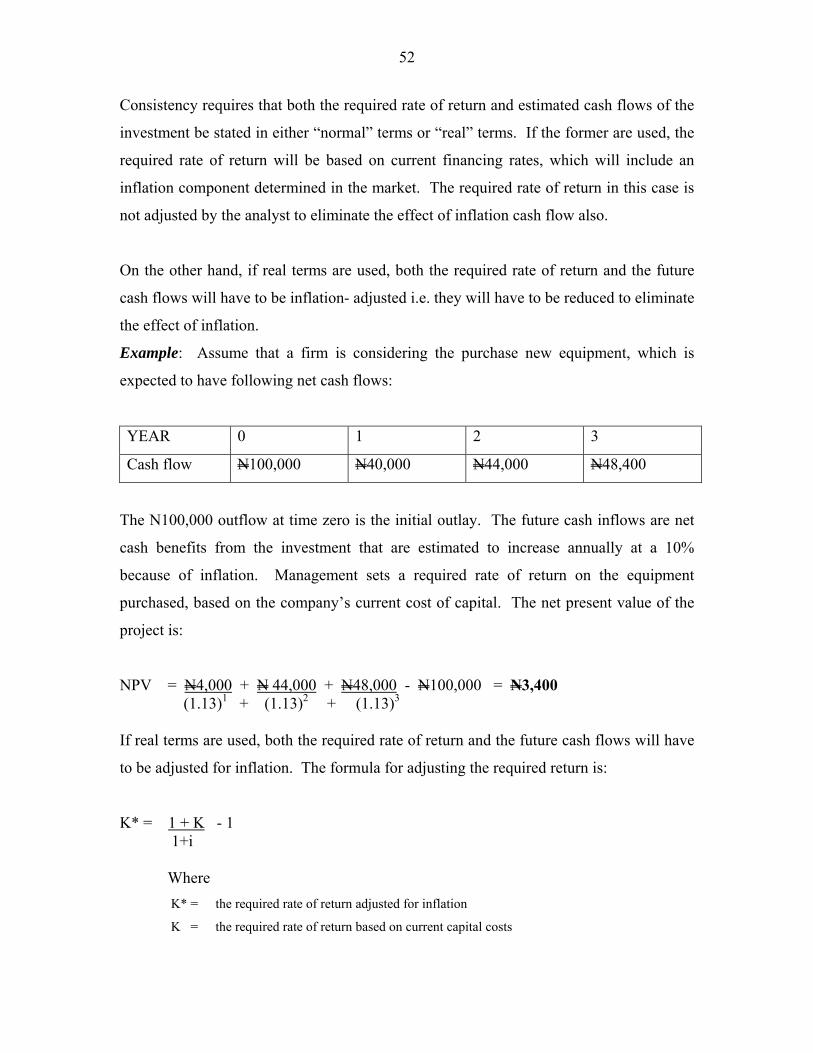
Example: Assume that a firm is considering the purchase new equipment, which is
expected to have following net cash flows:
YEAR 0 1 2 3
Cash flow N100,000 N40,000 N44,000 N48,400
The N100,000 outflow at time zero is the initial outlay. The future cash inflows are net
cash benefits from the investment that are estimated to increase annually at a 10%
because of inflation. Management sets a required rate of return on the equipment
purchased, based on the company’s current cost of capital. The net present value of the
project is:
NPV = N4,000 + N 44,000 + N48,000 - N100,000 = N3,400 (1.13)1 + (1.13)2 + (1.13)3
If real terms are used, both the required rate of return and the future cash flows will have
to be adjusted for inflation. The formula for adjusting the required return is:
K* = 1 + K - 1 1+i
Where
K* = the required rate of return adjusted for inflation
K = the required rate of return based on current capital costs
53
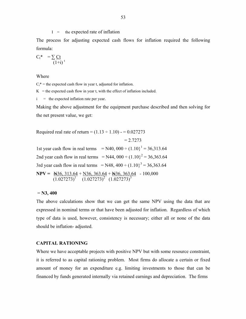
I = the expected rate of inflation
The process for adjusting expected cash flows for inflation required the following
formula:
Ct* = ∑ Ct
(1+i) t
Where
Ct* = the expected cash flow in year t, adjusted for inflation.
K = the expected cash flow in year t, with the effect of inflation included.
i = the expected inflation rate per year.
Making the above adjustment for the equipment purchase described and then solving for
the net present value, we get:
Required real rate of return = (1.13 ÷ 1.10) - = 0.027273
= 2.7273
1st year cash flow in real terms = N40, 000 ÷ (1.10}1 = 36,313.64
2nd year cash flow in real terms = N44, 000 ÷ (1.10}2 = 36,363.64
3rd year cash flow in real terms = N48, 400 ÷ (1.10}3 = 36,363.64
NPV = N36, 313.64 + N36, 363.64 + N36, 363.64 - 100,000 (1.027273)1 (1.027273)2 (1.027273)3
= N3, 400
The above calculations show that we can get the same NPV using the data that are
expressed in nominal terms or that have been adjusted for inflation. Regardless of which
type of data is used, however, consistency is necessary; either all or none of the data
should be inflation- adjusted.
CAPITAL RATIONING
Where we have acceptable projects with positive NPV but with some resource constraint,
it is referred to as capital rationing problem. Most firms do allocate a certain or fixed
amount of money for an expenditure e.g. limiting investments to those that can be
financed by funds generated internally via retained earnings and depreciation. The firms
54
must therefore ration them, allocating these funds to be in such a way the long run rate of
return is maximised.
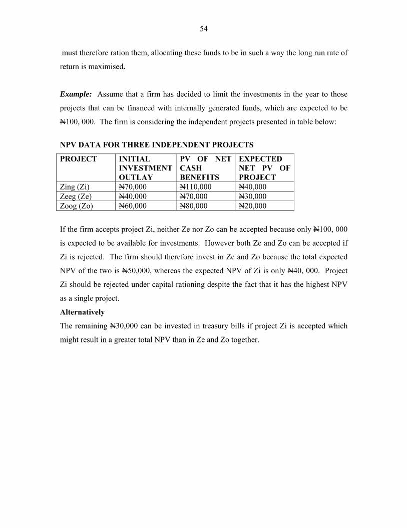
Example: Assume that a firm has decided to limit the investments in the year to those
projects that can be financed with internally generated funds, which are expected to be
N100, 000. The firm is considering the independent projects presented in table below:
NPV DATA FOR THREE INDEPENDENT PROJECTS
PROJECT INITIAL INVESTMENT OUTLAY
PV OF NET CASH BENEFITS
EXPECTED NET PV OF PROJECT
Zing (Zi) N70,000 N110,000 N40,000 Zeeg (Ze) N40,000 N70,000 N30,000 Zoog (Zo) N60,000 N80,000 N20,000
If the firm accepts project Zi, neither Ze nor Zo can be accepted because only N100, 000
is expected to be available for investments. However both Ze and Zo can be accepted if
Zi is rejected. The firm should therefore invest in Ze and Zo because the total expected
NPV of the two is N50,000, whereas the expected NPV of Zi is only N40, 000. Project
Zi should be rejected under capital rationing despite the fact that it has the highest NPV
as a single project.
Alternatively
The remaining N30,000 can be invested in treasury bills if project Zi is accepted which
might result in a greater total NPV than in Ze and Zo together.
55
CAPITAL BUDGETING UNDER RISK
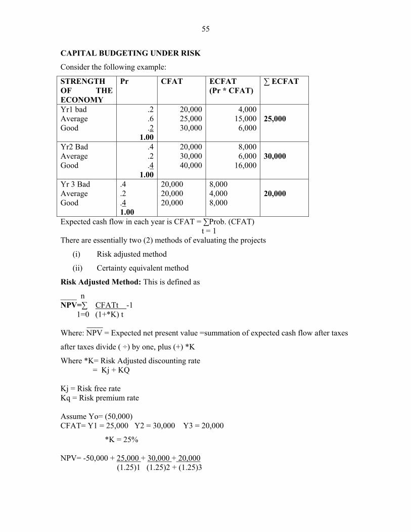
Consider the following example:
STRENGTH OF THE ECONOMY
Pr CFAT ECFAT (Pr * CFAT)
∑ ECFAT
Yr1 bad Average Good
.2
.6
.2 1.00
20,00025,00030,000
4,00015,0006,000
25,000
Yr2 Bad Average Good
.4
.2
.4 1.00
20,00030,00040,000
8,0006,000
16,000
30,000
Yr 3 Bad Average Good
.4
.2
.4 1.00
20,000 20,000 20,000
8,000 4,000 8,000
20,000
Expected cash flow in each year is CFAT = ∑Prob. (CFAT) t = 1 There are essentially two (2) methods of evaluating the projects
(i) Risk adjusted method
(ii) Certainty equivalent method
Risk Adjusted Method: This is defined as
____ n NPV=∑ CFATt -1 1=0 (1+*K) t ____ Where: NPV = Expected net present value =summation of expected cash flow after taxes
after taxes divide ( ÷) by one, plus (+) *K
Where *K= Risk Adjusted discounting rate = Kj + KQ Kj = Risk free rate Kq = Risk premium rate Assume Yo= (50,000) CFAT= Y1 = 25,000 Y2 = 30,000 Y3 = 20,000
*K = 25% NPV= -50,000 + 25,000 + 30,000 + 20,000 (1.25)1 (1.25)2 + (1.25)3
56
= (50,000) + 25,000 (0.8) + 30,000 (0.64) + 20,000 (0.512) = (50,000) + 20,000 + 19,200 + 10,240 = -560 or (560) This technique is found to be useful and has the following merit.
(i) Simple to calculate
(ii) It has a great deal of intuitive appeal for risk- adverse investors.
Demerits:
(i) No easy way to arrive at a risk adjusted discounting rate. The risk free is already
known. It is the risk rate that is difficult t determine.
(ii) It does not make any risk adjustment in the numerator.
(iii) It is based on the assumption that all investors are risk- averse – some are risk-
seekers.
Certainty – Equivalent Technique
Here, the riskness of each project is handled by adjusting the expected cash flow and not
by adjusting the discounting rate.
n n NPV =∑ t CFATt = ∑ CEt t=0 (1+Kj) t=0 (1+Kj) t Where: CEt = Certainty Equivalent of CFATt = Ł CFATt
Ł = Certainty Equivalent factor for 1 year which is always bet 0-1
NB: Where there is no risk at all, Certainty Equivalent factor = 1
Kj = Risk free interest rate.
57
Assume the following Kj = 13%
Ł1=0.90 Ł2 = 0.70 Ł3 =0.60
NPV = -50.000 + 0.90(25,000) + 0.70(30,000) +0.60(20,000 (1.13)1 (1.13)2 (1.13)3 = 0.88496(22,500) = 19,911.60 0.78315(21,000) = 16,446.20 0.69305(12,000) = 8,316.60 44,674.4 -50,000
(5325.6) -Reject.
SELECTED PAST QUESTIONS
1. (a) Explain why capital budgeting decisions are the most difficult decisions to make.
(b) The management of London Chambers has decided to purchase a set of computer
for its use. The alternatives have been narrowed down to two models. Model PK, and
Model PC, costing only N95, 000.00 and N60, 000.00 respectively. The net cash benefits
from PK are estimated at N30, 000.00 a year for 5 years, whereas the benefits from PC
are estimated at N25, 000.00 a year for three years. The salvage value is estimated at
N15, 000 and N12, 000.00 respectively. The selected project is to be financed by issuing
a twenty-year bond whose interest rate will be 20%. The company’s marginal income tax
-rate is 30%. Which project should be selected and why?
2(a) Briefly explain the types of capital budgeting decisions you are familiar with.
(b) Assume that the market price of the Ka’oje Company’s stock is N40. The
dividend payable at the end of the coming year is N4 per share and is expected to
grow at a constant annual rate of 6 percent. What is the cost of this external
equity capital?
(c) Cronosoft.Com has a fixed budget of N250, 000. The company needs to select a
mix of acceptable projects from the following:
PROJECTS INITIAL INVESTMENT (N) PRESENT VALUE (N) XP Visual Tools 70,000 112,000 Add XP 100,000 145,000 Boot XP 110,000 126,500 Logon UI 60,000 79,000 Fresh Devices 40,000 38,000 Charger XP 80,000 95,000
58
Based on these data:
(a) Compute the Net Present Value (NPV) of each project. (b) Rank these five projects in the descending order of preference
Which projects would you select given the fixed budget? 3. Kalambaina Textile Ltd is proposing to invest in Arkilla-Classic Print costing
N6,000,000. The project is expected to have a life of four (4) years with a nil residual
value. The net cash flows from the project are uncertain but the likelihood of their
occurrence is given as follows:
Year 1 Year 2 Year 3 Year 4 Cash flow ‘000
Probability Cash flow ‘000
Probability Cash flow ‘000
Probability Cash flow ‘000
Probability
2,000 0.2 2,500 0.4 4,000 0.3 2,000 0.45 1,500 0.4 2,800 0.3 3,000 0.35 6,050 0.15 1,800 0.3 3,000 0.2 4,500 0.25 5,000 0.2 3,000 0.1 3,500 0.1 5,000 0.1 4,500 0.2 The Treasury bill rate is currently 12% per annum and the company requires a risk
premium of 5% to compensate risk -ness of this project.
REQUIRED:
(a) Using the Risk Adjusted method, should the project be accepted?
(b) If the certainty- equivalent-coefficient is 1.00. 0.9. 0.8 and 0.6 for year 1,2,3
and 4 respectively, should the proposal be accepted using the Certainty-
Equivalent approach?
What are the demerits of Risk Adjusted method?
59
COST OF CAPITAL
It is a decision criterion to be used by the management of the enterprise.
Its basic intent is to provide a defensible answer to the question.
What rate of return must an investment promise to deliver in order that the
firm’s owners will be no better or work off in a monetary sense if the
investment is undertaken?
It is thus an aid in determining whether acceptance of a specific project
will provide an economic benefit in the firm’s owners.
A proposed use of corporate funds must earn a rate of return greater than
the cost of the funds that the project employ or the market price of the
firm’s common stock will be adversely affected.
It is defined as the minimum rate of return that must be earned on an
investment in order to leave the market price of the firm’s common stock
unchanged.
COSTS OF INDIVIDUAL SOURCES OF CAPITAL
Major avenues of long-term financing available to the firm include:
Debt
Preferred stock
Equity/Retains Earnings
Convertible securities
Common Stock
Warrantees/Leases
Methods for approximating the cost of some of these sources of capital is explained and
illustrated below:
Cost of Long term Debt
A firm incurs long-term debt by selling bonds to investor who desire to purchase fixed
income securities and retain the position of a creditor rather than an equity investor in the
organisation. Although there are different types of bonds, they however have certain
common elements that permit their cost to be estimated. These include:
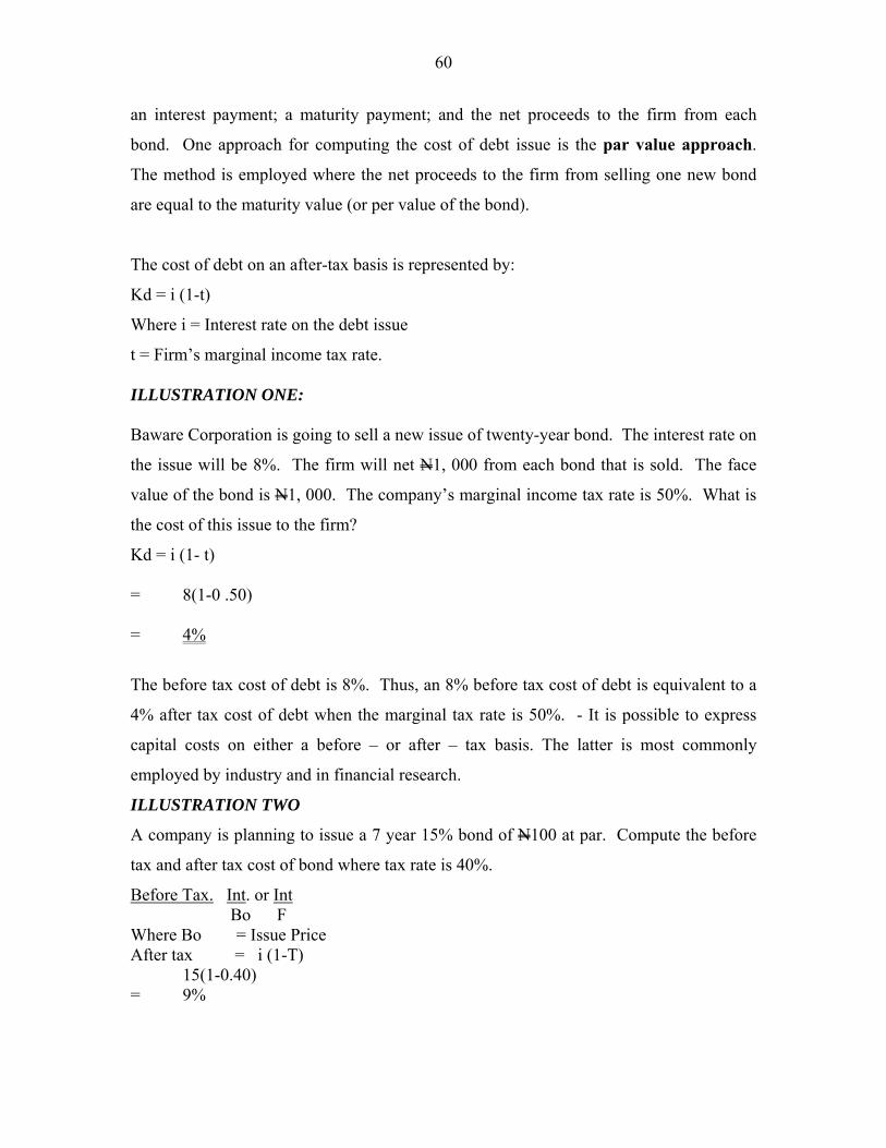
60
an interest payment; a maturity payment; and the net proceeds to the firm from each
bond. One approach for computing the cost of debt issue is the par value approach.
The method is employed where the net proceeds to the firm from selling one new bond
are equal to the maturity value (or per value of the bond).
The cost of debt on an after-tax basis is represented by:
Kd = i (1-t)
Where i = Interest rate on the debt issue
t = Firm’s marginal income tax rate.
ILLUSTRATION ONE: Baware Corporation is going to sell a new issue of twenty-year bond. The interest rate on
the issue will be 8%. The firm will net N1, 000 from each bond that is sold. The face
value of the bond is N1, 000. The company’s marginal income tax rate is 50%. What is
the cost of this issue to the firm?
Kd = i (1- t) = 8(1-0 .50) = 4%
The before tax cost of debt is 8%. Thus, an 8% before tax cost of debt is equivalent to a
4% after tax cost of debt when the marginal tax rate is 50%. - It is possible to express
capital costs on either a before – or after – tax basis. The latter is most commonly
employed by industry and in financial research.
ILLUSTRATION TWO
A company is planning to issue a 7 year 15% bond of N100 at par. Compute the before
tax and after tax cost of bond where tax rate is 40%.
Before Tax. Int. or Int Bo F Where Bo = Issue Price After tax = i (1-T)
15(1-0.40) = 9%
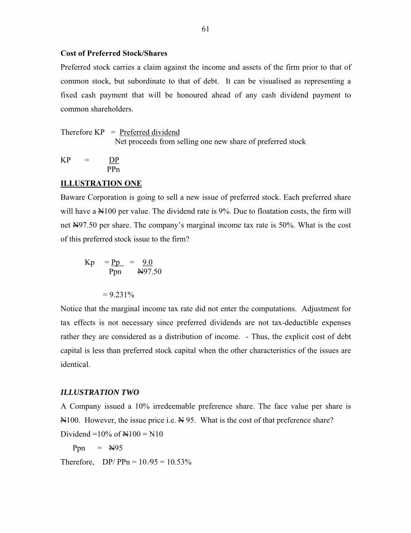
61
Cost of Preferred Stock/Shares
Preferred stock carries a claim against the income and assets of the firm prior to that of
common stock, but subordinate to that of debt. It can be visualised as representing a
fixed cash payment that will be honoured ahead of any cash dividend payment to
common shareholders.
Therefore KP = Preferred dividend Net proceeds from selling one new share of preferred stock KP = DP PPn
ILLUSTRATION ONE
Baware Corporation is going to sell a new issue of preferred stock. Each preferred share
will have a N100 per value. The dividend rate is 9%. Due to floatation costs, the firm will
net N97.50 per share. The company’s marginal income tax rate is 50%. What is the cost
of this preferred stock issue to the firm?
Kp = Pp = 9.0 Ppn N97.50
= 9.231%
Notice that the marginal income tax rate did not enter the computations. Adjustment for
tax effects is not necessary since preferred dividends are not tax-deductible expenses
rather they are considered as a distribution of income. - Thus, the explicit cost of debt
capital is less than preferred stock capital when the other characteristics of the issues are
identical.
ILLUSTRATION TWO
A Company issued a 10% irredeemable preference share. The face value per share is
N100. However, the issue price i.e. N 95. What is the cost of that preference share?
Dividend =10% of N100 = N10
Ppn = N95
Therefore, DP/ PPn = 10 ⁄95 = 10.53%
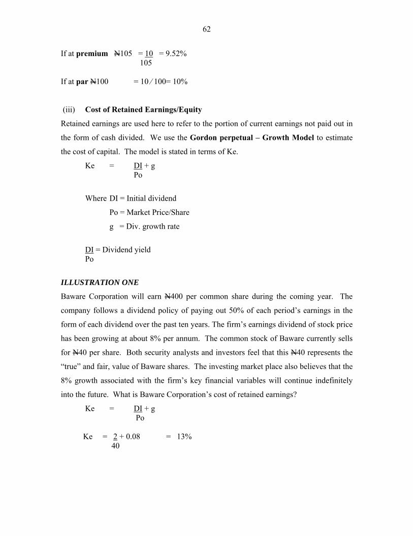
62
If at premium N105 = 10 = 9.52% 105 If at par N100 = 10 ⁄ 100= 10%
(iii) Cost of Retained Earnings/Equity
Retained earnings are used here to refer to the portion of current earnings not paid out in
the form of cash divided. We use the Gordon perpetual – Growth Model to estimate
the cost of capital. The model is stated in terms of Ke.
Ke = DI + g Po
Where DI = Initial dividend
Po = Market Price/Share
g = Div. growth rate
DI = Dividend yield Po
ILLUSTRATION ONE
Baware Corporation will earn N400 per common share during the coming year. The
company follows a dividend policy of paying out 50% of each period’s earnings in the
form of each dividend over the past ten years. The firm’s earnings dividend of stock price
has been growing at about 8% per annum. The common stock of Baware currently sells
for N40 per share. Both security analysts and investors feel that this N40 represents the
“true” and fair, value of Baware shares. The investing market place also believes that the
8% growth associated with the firm’s key financial variables will continue indefinitely
into the future. What is Baware Corporation’s cost of retained earnings?
Ke = DI + g Po
Ke = 2 + 0.08 = 13% 40
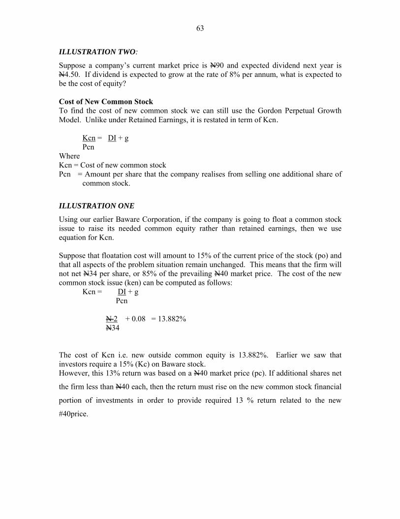
63
ILLUSTRATION TWO:
Suppose a company’s current market price is N90 and expected dividend next year is N4.50. If dividend is expected to grow at the rate of 8% per annum, what is expected to be the cost of equity? Cost of New Common Stock To find the cost of new common stock we can still use the Gordon Perpetual Growth Model. Unlike under Retained Earnings, it is restated in term of Kcn.
Kcn = DI + g Pcn
Where Kcn = Cost of new common stock Pcn = Amount per share that the company realises from selling one additional share of
common stock.
ILLUSTRATION ONE
Using our earlier Baware Corporation, if the company is going to float a common stock issue to raise its needed common equity rather than retained earnings, then we use equation for Kcn. Suppose that floatation cost will amount to 15% of the current price of the stock (po) and that all aspects of the problem situation remain unchanged. This means that the firm will not net N34 per share, or 85% of the prevailing N40 market price. The cost of the new common stock issue (ken) can be computed as follows:
Kcn = DI + g Pcn
N 2 + 0.08 = 13.882% N34
The cost of Kcn i.e. new outside common equity is 13.882%. Earlier we saw that investors require a 15% (Kc) on Baware stock. However, this 13% return was based on a N40 market price (pc). If additional shares net
the firm less than N40 each, then the return must rise on the new common stock financial
portion of investments in order to provide required 13 % return related to the new
#40price.
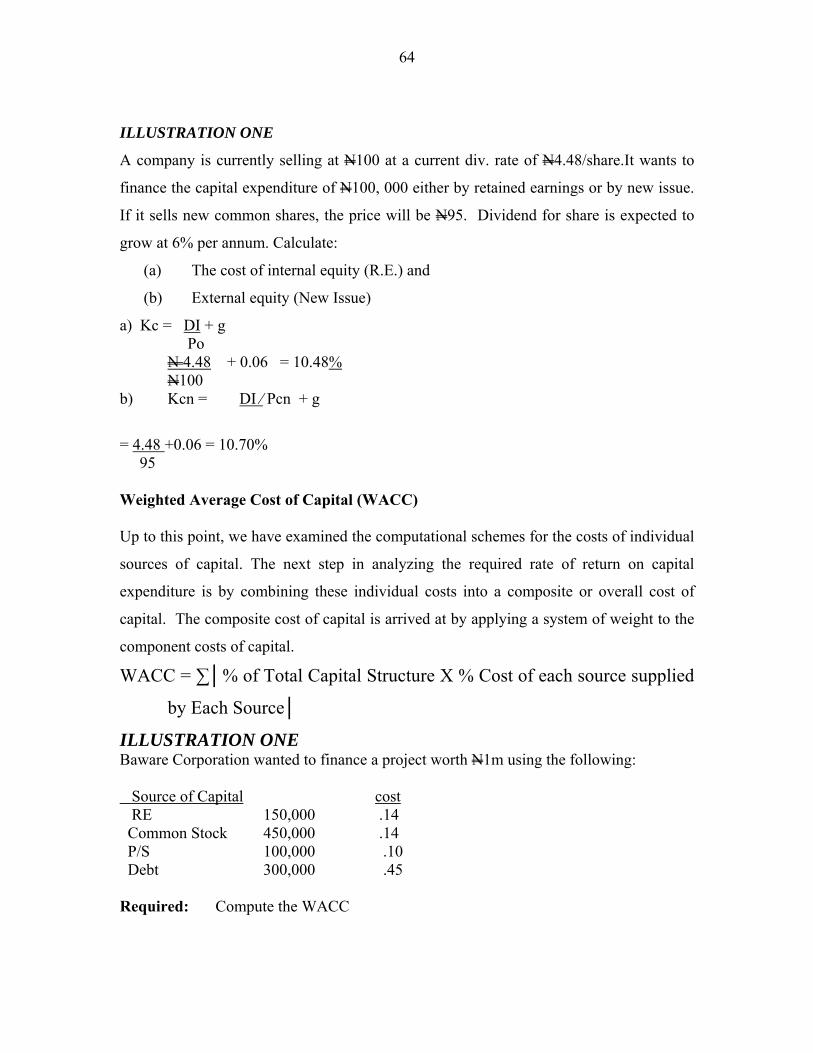
64
ILLUSTRATION ONE
A company is currently selling at N100 at a current div. rate of N4.48/share.It wants to
finance the capital expenditure of N100, 000 either by retained earnings or by new issue.
If it sells new common shares, the price will be N95. Dividend for share is expected to
grow at 6% per annum. Calculate:
(a) The cost of internal equity (R.E.) and
(b) External equity (New Issue)
a) Kc = DI + g Po N 4.48 + 0.06 = 10.48% N100
b) Kcn = DI ⁄ Pcn + g
= 4.48 +0.06 = 10.70% 95 Weighted Average Cost of Capital (WACC) Up to this point, we have examined the computational schemes for the costs of individual
sources of capital. The next step in analyzing the required rate of return on capital
expenditure is by combining these individual costs into a composite or overall cost of
capital. The composite cost of capital is arrived at by applying a system of weight to the
component costs of capital.
WACC = ∑│% of Total Capital Structure X % Cost of each source supplied
by Each Source│
ILLUSTRATION ONE Baware Corporation wanted to finance a project worth N1m using the following: Source of Capital cost RE 150,000 .14 Common Stock 450,000 .14 P/S 100,000 .10 Debt 300,000 .45 Required: Compute the WACC
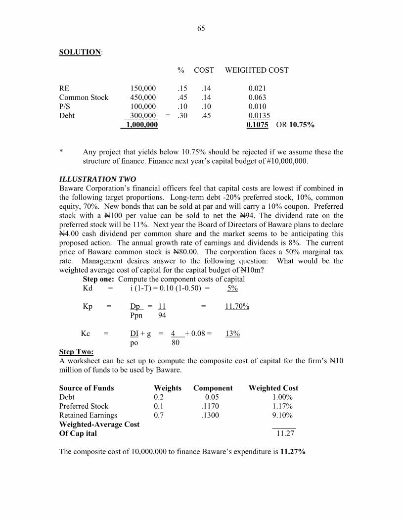
65
SOLUTION: % COST WEIGHTED COST RE 150,000 .15 .14 0.021 Common Stock 450,000 .45 .14 0.063 P/S 100,000 .10 .10 0.010 Debt 300,000 = .30 .45 0.0135 1,000,000 0.1075 OR 10.75% * Any project that yields below 10.75% should be rejected if we assume these the
structure of finance. Finance next year’s capital budget of #10,000,000. ILLUSTRATION TWO Baware Corporation’s financial officers feel that capital costs are lowest if combined in the following target proportions. Long-term debt -20% preferred stock, 10%, common equity, 70%. New bonds that can be sold at par and will carry a 10% coupon. Preferred stock with a N100 per value can be sold to net the N94. The dividend rate on the preferred stock will be 11%. Next year the Board of Directors of Baware plans to declare N4.00 cash dividend per common share and the market seems to be anticipating this proposed action. The annual growth rate of earnings and dividends is 8%. The current price of Baware common stock is N80.00. The corporation faces a 50% marginal tax rate. Management desires answer to the following question: What would be the weighted average cost of capital for the capital budget of N10m?
Step one: Compute the component costs of capital Kd = i (1-T) = 0.10 (1-0.50) = 5% Kp = Dp = 11 = 11.70% Ppn 94
Kc = DI + g = 4 + 0.08 = 13%
po 80 Step Two: A worksheet can be set up to compute the composite cost of capital for the firm’s N10 million of funds to be used by Baware. Source of Funds Weights Component Weighted Cost Debt 0.2 0.05 1.00% Preferred Stock 0.1 .1170 1.17% Retained Earnings 0.7 .1300 9.10% Weighted-Average Cost ______ Of Cap ital 11.27 The composite cost of 10,000,000 to finance Baware’s expenditure is 11.27%
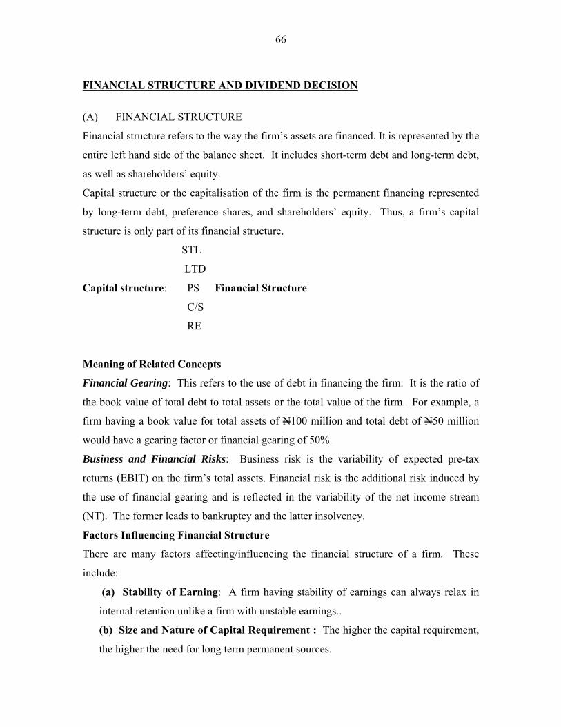
66
FINANCIAL STRUCTURE AND DIVIDEND DECISION
(A) FINANCIAL STRUCTURE
Financial structure refers to the way the firm’s assets are financed. It is represented by the
entire left hand side of the balance sheet. It includes short-term debt and long-term debt,
as well as shareholders’ equity.
Capital structure or the capitalisation of the firm is the permanent financing represented
by long-term debt, preference shares, and shareholders’ equity. Thus, a firm’s capital
structure is only part of its financial structure.
STL
LTD
Capital structure: PS Financial Structure
C/S
RE
Meaning of Related Concepts
Financial Gearing: This refers to the use of debt in financing the firm. It is the ratio of
the book value of total debt to total assets or the total value of the firm. For example, a
firm having a book value for total assets of N100 million and total debt of N50 million
would have a gearing factor or financial gearing of 50%.
Business and Financial Risks: Business risk is the variability of expected pre-tax
returns (EBIT) on the firm’s total assets. Financial risk is the additional risk induced by
the use of financial gearing and is reflected in the variability of the net income stream
(NT). The former leads to bankruptcy and the latter insolvency.
Factors Influencing Financial Structure
There are many factors affecting/influencing the financial structure of a firm. These
include:
(a) Stability of Earning: A firm having stability of earnings can always relax in
internal retention unlike a firm with unstable earnings..
(b) Size and Nature of Capital Requirement : The higher the capital requirement,
the higher the need for long term permanent sources.
67
(c) Management attitudes – The management attitudes that will directly influence
the choice of financing are those concerning:
(i) Control of the enterprise and
(ii) Risk
(i) Control of the Enterprise: Large companies whose shares are widely owned
may choose additional sales of ordinary shares because such sales will have
little influence on the control of the company. In contrast, the owners of small
firms may prefer to avoid issuing ordinary shares in order to be assured of
continued control.
(ii) Risk: Some managers are more conservative than others so that they may
decide to limit the use of debt, which increases the risk of losing a substantial
portion of their wealth.
(d) Suitability of Funds to Assets: The principle of suitability states that there
should be a kind of matching e.g. current assets financing with short-term
loans and fixed assets with long-term loan and equity.
(e) Lenders’ Attitudes: Lenders attitudes determine financial structure regardless
of managements’ views. For instance, if management seeks to use gearing
beyond norms for the industry, lenders may be unwilling to accept such debt
increases. They emphasize that excessive debt reduces the credit standing of
the borrower and the credit rating of the securities previously issued.
(f) Government Regulation: Example of this is where government may say
that the equity ratio of a firm should not be more than a certain amount. Thus,
a firm has to borrow to finance other investments.
Others include interest rate, investors’ attitudes, flexible nature of the source etc. etc.
Importance of managing the Financial Structure
(a) Not all capital sources cost the same. For instance, debt costs more than preference
and common shares. Therefore, since this is the case and since their costs do not remain
fixed through time, then constant monitoring of the firm’s financial structure is necessary
68
in order to detect opportunities to substitute lower cost forms of capital funds from costly
ones.
(b) The opportunity to use the benefit of leverage and to ensure the possibilities for over-
use of leverage are not incurred. This is one of the tools of managing the financial
structure. In finance, leverage refers to the magnification of profit by the
employment of assets and financing that have fixed costs.
LEVERAGE AND CAPITAL STRUCTURE
Leverage is that portion of fixed costs which represents a risk to the firm. There are three
types of leverages: operating; financial; and combined.
Operating leverage is a measure of operating risk which refers to the fixed operating
costs found in a firm’s income statement. It is the responsiveness of the firm’s EBIT or
operating income to changes in sales. It results from the presence of fixed operating costs
in the firm’s cost structure. The degree of operating leverage is used to measure the
percentage change in operating income to the percentage change in units sold or in total
revenue. A high degree of operating leverage implies that a relatively small change in
sales results in a large change in not operating income. Algebraically DOL is defined as:
Percentage change in operating income = % ∆ in EBIT Percentage change in units sold or in TR % ∆ in sales
∆ Income/Income = ∆X/X = (P-V) X ∆Q/Q ∆Q/Q (P-V) X-FC
= Q(S-V) = EBIT = Contr. Q(S-V)-F ∆ Sales EBIT
Sales
To illustrate DOL, consider the following income statement of Dandima Development
Company
Selling Price = N2
Fixed Costs = N 20,000
Variable Costs = N1.50Q
69
UNITS SOLD SALES N COST N OPERATING INCOME N 20,000 40,000 50,000 - 10,000 40,000 80,000 80,000 0 UNDEFINED 60,000 120,000 110,000 10,000 3.03 80,000 160,000 140,000 20,000 2.00 100,000 200,000 170,000 30,000 1.67 120,000 240,000 200,000 40,000 1.50 200,000 400,000 320,000 80,000
For this company, the degree of operating expenses for a change in units is
DOL = ∆X = N 40,000 – 30,000 X __30,000__ ∆Q N 120,000 – 100,000 X 100,000 = 10,000
30,000 = 33.33% = 1.67 20,000 20%
100,000
OR
DOL = Q (P-V)
Q (P-V)-F
Where P = Price per Unit
V = Variable cost per unit
F = Total Fixed Cost
DOL = 100,000 (2-1.5)
100,000 (2-1.5) – 20,000
= 50,000 =1.67 30,000
Therefore, a change from 100,000 to 120,000 or 20% increase in sales will lead to a
16.7% increase in operating income. Correspondingly, a 20% drop in sales would cause
operating to drop by 16.7%.
70
The significance of this is that as a firm’s sales move above the break-even point, the
degree of operating leverage at each higher sales base declines. The greater the sales
level (above the BEP), the lower the degree of operating leverage. For Dandima
Development Company, at the BE sales level, the denominator in any of the
computational formulae is 0 beyond the break-even point of 40,000 units, the DOL
declines. It will decline at a decreasing rate and approach a value of 1.00. As long as
some fixed operating costs are present in the firm’s cost structure, however, operating
leverage exists and DOLS will exceed 1.00.
Consider another illustration: the Dundaye Corporation produces tea-kettles, which it
sells for N10. Fixed costs are N600, 000 for up to 400, 000 units of output. Variable
costs are N7 per unit.
(a) What is the firm’s gain or loss at sales of 175,000 units? Of 300,000 units?
(b) What is the break-even point?
(c) What is Dundaye’s degree of operating leverage of sales of 225,000 units? of
300,000 units?
(a) (I) At sales of 175,000 units TR = 10 X 175,000 = N1, 750,000 TC = 600,000 + (7X 175,000) = N1, 825,000 Profit/Loss = TR - TC 1,750,000 – 1,825,000 Loss = (N 75,000) (ii) At Sales of 300,000 Units TR = 10 X 300,000 = N3, 000,000 TC = 600,000 + (7 x 300,000) = 2,700,000
Profit/Loss = TR – TC
3,000,000 – 2,700,000
Profit = N300, 000
71
(b) BEP = __ FC = 600,000 = 200,000 units SP/U – VC/U 10-7 BEP = 200,000 x 10 = N2, 000,000
(c) DOL (i) At Sales of 225,000 units DOL = Q (P-V) (P-V) – F 225,000(10-7) 225,000 (10-7) – 600,000
675,000 75,000 = 9 or 9%
(ii) Of 300,000 units
300,000 (10-7) 300,000 (10-7) – 600,000 900,000 = 3 or 30% 300,000 12.5% increase in sales will lead to a 90% in operating income.
Financial leverage, a measure of financial risk, refers to financing a portion of the firm’s
assets, bearing fixed financing charges in hopes of increasing the return to the common
stockholders. That is, financing with sources of capital that have fixed charges that must
be met example debt, preferred stock etc. these financing fixed costs provide the same
magnification effect on the firm’s earnings per share (EPS) that operating fixed costs
have on earning before interest and taxes (EBIT). The more fixed charge financing the
firm uses, the more financial leverage it will have. The higher the financial leverage, the
higher the financial risk, and the higher the cost of capital rises because it costs more too
raise funds for a risky business. Algebraically DFL is defined as:
72
DFL = % in EPS = ∆EPS = EBIT % in EBIT EPS EBIT – INT ∆ EBIT EBIT
Combined Leverage is simply a combination of operating leverage with financial
leverage. Degree of combined leverage is therefore defined as:
DCL = DOL x DFL Q(S-V) x Q(S-V) - F Q(S-V)-F Q(S-V) – F - Interest
ILLUSTRATION A company that has current total sales of 250,000 units, variable cost per unit is N2.50 and sells (S.P. /U) is N5.00. Its fixed costs are N100, 000 and interest charges at N50, 000. Compute the DOL, DFL and DCL and comment on the risk situation of the firm. SOLUTION: Sales = 250,000 @ N5 1,250,000 Less Variable Cost = 250,000 @ N2.50 625,000 Contribution = 625,000 Less Fixed Cost = 100,000 EBIT 525,000 DOL = Contr. = 625,000 = 1.19% EBIT 525,000 Any one Naira (N1.00) change in sales will bring 1.19 changes in EBIT. DFL = EBIT = 525,000 = 1.105% EBIT- INT 525,000 – 50,000 Any N1 change in EBIT results in 1.05 change in earning per share.
DCL = DOL X DFL = 1.19 X 1.105 = 1.32%
73
Optimal capital structure –: Maximizes the market value of the firm through an
appropriate mix of long term financing. Sources of funds-: Minimize the firm’s overall
cost of capital. There are four different approaches to the theory of capital structure.
These are: Net Operating Income (NOI); Net Income (NI); Traditional; and Modigliani-
Miller (MM).
REVISION QUESTIONS
1. Takalmawa Plc. located at Marina square is a producer of plastic materials. The
company has idle capacity and provided the following data:
SP/u = N80 VC/u = = N 50
FC/u = N10 Annual credit Sales = 300,000.00 units
Collection period = 2 months, Rate of Return = 13%
The corporation is considering a change in policy that will relax its credit standards. The
following information applies to the proposal:
(a) Sales will increase by 25%
(b) Collection period will go to 6 months.
(c) Bad debt losses are expected to be 5% of the increased sales
(d) Collection costs are expected to increase by N35,000.00
Required:
Provide an analysis of its proposed credit policy change. Should Takalmawa Plc accept the proposal and why?. 2 (a) Briefly comment on the short-comings of the ZETA model of prediction of
financial distress.
(b)Two companies have the following financial characteristics (in thousands Naira)
Zamko Company Kebko Company Working Capital 21,000 4,000 Total Assets 100,000 42,000 Total liabilities 44,000 26,000 Equity Value (mrk) 76,000 45,500 Retained Earnings 38,000 6,000 Sales 172,000 55,000 Earning before interest 24,000 3,000
74
and taxes Common Stock 300,000 175,000
Required:
(i) Compute for each Altman’s Z Score Index
(ii) Based on these indices, is either company likely to go into bankruptcy? Why?
3 (a) Distinguish between financial and business risks.
(b) Maishanu & Daughters PLC sells new shares of common stock at N35, 000.
The floatation cost is 10%. Both earnings and dividends are expected to
grow at a constant rate of 6 percent and the annual dividend per share is
N4.00. What is the cost of external equity?
(c) John Tripper Soft Drinks Plc sells 500,000 bottles of soft drinks a year.
Each bottle produced has a variable cost of N0.25, sells for N0.45. Fixed
operating costs are N50, 000.00. The company has current interest charges
of N6, 000.00 and preferred dividends of N2, 400.00 and the company faces
40% tax bracket. You are required to compute the following:-
(i) Break even point (units and Naira) (ii) Degree of operating leverage (iii) Degree of financial leverage (iv) Degree of total leverage (v) Do part (i) to (iv) at the 750,000 bottle sales level?
4. Ina Kwana, Ina Yini Corporation is thinking of purchasing a new machine. With
this new machine, the Company expects sales to increase from N8, 000,000.00 to N10, 000,000.00 The Company knows that its assets, accounts payable and accrued expenses vary directly with sales. The Company’s profit margin on sales is 8 percent, and it plans to pay 40 percent of its after- tax earnings in dividends. The Company’s current balance sheet is given below
Balance sheet N Current Assets 3,000,000 Fixed Assets 12,000,000 Total Assets 15,000,000 Accounts Payable 4,000,000 Accrued expenses 1,000,000 Long-term Debt 3,000,000
75
Common Stock 2,000,000 Retained Earnings 5,000,000 15,000,000
REQUIRED: Determine the following:
(a) The external funds needed by the company
(b) The external funds needed if profit margin is 8 percent, but the dividend
payout ratio reduced from 40 percent to 20 percent.
(c) If profit margin rises from 8 percent to 10 percent, at what growth rate in sales
will the percentage of the external financing requirement be exactly zero?
5. We- don -Win Ltd reports the following information:
Selling price per unit N70
Variable cost per unit N 45
Fixed cost per unit N 15
Annual cost per unit 400,000 units
Collection period 3 months
Rate of returns. 19%.
The company is considering easing its credit standards. If it does, the following is
expected to result: Sales will increase by 25 percent; collection period will
increase to 4 months; bad debts losses are anticipated to be 4 percent on the
incremental sales, and collection costs will increase by N34, 000.00.
Should the proposed relaxation in credit standards be implemented?
6 (a) Briefly highlight the main features of Edward Altman’s Discriminant
Analysis Model
(b) The following represents the financial ratios of Temper-Justice with
Mercy plc.
Working capital to Total Asset = 7.62%
EBIT to Total Asset = 6.2%
76
Sales to Total Asset = 1.095 times
Retained Earnings to Total Assets = 14.3%
Market value of Equity to Book Value of Debt = 39.2%
You are required to:
(i) Compute for the company Altman’s Z-Score Index
(ii) On the basis of these ratios, is the company likely to go into
bankruptcy? Why?
7. (a) Temper Justice with Mercy (TJWM) Ltd sells 500,000 bottles of Sobo drinks a
year. Each bottle produced has a variable cost of N0.25 sells for N0.45. Fixed
operating costs are N50, 000.00. The company has current interest charges of N6,
000.00 and preferred dividends of N2, 400.00. The corporate tax rate is 40
percent.
(a) Calculate the Break-Even Point in units and Naira
(b) Calculate the degree of operating leverage degree of financial
leverage, and the degree of combine leverage
(c) Do part (a) at the 750,000 bottles sales ( 9 Marks)
(b) Von Voyage Transportation Ltd has estimated cash payments of N4,
000,000 for a three-month period. Cash payments are expected to be steady over
the period. Fixed cost per transactions is N200 and the interest rate on treasury
bills is 10% per annum. Calculate the optional cash level and the total cost of
cash management policy over the three-month period.
8. (a) Enumerate four(4) different approaches to the theory of capital structure
(b) Bin Laden Corporation has the following capital structure, which it
considers optimal:
Bonds, 7% (now selling at par N300, 000
Preferred Stock (N5 dividend) 240,000
Common Stock 360,000
Retained Earnings 300,000 1,200,000
77
Dividends on common stock are currently N3 per share and are expected
to grow at a constant rate of 6 percent. Market price per share of common
stock is N40, and the preferred stock at N50. Floatation cost on new
issues of common stock is 10 percent. The interest on bonds is paid
annually. The company’s tax rate is 40 percent.
Calculate (a) The before-and after tax cost of bonds (b) The cost of
preferred stock (c) The cost of retained earnings (d) The cost of new
common stock, and (e) The weighted average cost of capital.
9. Sadaqatul Jariyat Corporation has an annual sales of 120,000 units which
generate sales revenue of N2, 400,000 and an average collection period of
30 days. It is considering a more liberal credit policy. If the credit period
is extended, the corporation expects (other things being equal) sales and
bad debt losses to increase in the following manner:
You are given the following additional information: Policy X Policy Y Present Policy Additional Sales - Bad debt risk (as % of sales)
1 Average Collection Period
1 month
Collection cost N20,000 N30,000
(i) The Corporation’s expected return on investment is 25% (ii) Unit cost N15,000 (iii) Variable cost/unit N12,000 (iv) No increase in fixed cost, average stocks, and taxes from the extra
turnover (v) All sales are on credit (vi) A-360-day-year is assumed.
REQUIRED: Advice the firm
10 a. Briefly explain ‘credit standard’ and ‘credit terms’.
b. The RIKICI-RIGIMA Corporation has annual sales of 2.4 million
and an average collection period of 30 days. It is considering a
78
more liberal credit policy. If the credit period is extended, the
Corporation expects (other things being equal) sales and bad debt
losses to increase in the following manner:
Variables Present Policy
Policy A Policy B
Additional Sales - 25% 35% Average Collection Period
1 month 2 months 3 months
Bad Debt Risk (As % of sales)
1 3 6
You are given the following additional information:
The Corporation’s expected return on investment 25%
* Selling price per unit N20.00
* Average cost per unit N15.00
* Variable cost per unit N12.00
* No increase in fixed costs, average stocks and taxes from
the extra turnover
* All sales on credit
* A-360-day-year is assumed.
Required:
Advice, RIKICI-RIGIMA on the preferable credit policy.
11. Companies U and L are identical in every respect except that U is unlevered while
L has N10, 000,000 of 5% bonds outstanding. Assume (i) that all of MM
assumptions are met. (ii) That the tax rate s 40 %.( iii) that EBIT is N 2,000,000
(iv) that the equity capitalisaton rate for Company U is 10%, and (v) that the
coupon rate is equal to the risk- free rate. i.e., 5%.
Required:
(a) What value would MM estimate for each firm?
79
(b) Suppose Vu = N 8,000,000 and VL = N18, 000,000. According too MM, do
these represent equilibrium values? If not, explain the process by which
equilibrium will be restored. No calculations are necessary.
12. The Balewa Company Ltd, plans to issue 20-year bonds that have a 10 percent
Coupon, a pair value of N 1,000 and can be sold for N 920. Interest is paid semi-
annually. Balewa’s tax rate is 40%.
(a) What is the after -tax cost of this debt to Balewa?
(b) What would be the after -tax cost if this were a perpetual bond issue?