1

MGT 821/ECON 873 Numerical Procedures

2

Approaches to Derivatives Approaches to Derivatives ValuationValuation

How to find the value of an option? Black-Scholes partial differential equation Risk neutral valuation

Analytical solution Numerical methods

Trees Monte Carlo simulation Finite difference methods

3

Binomial Trees

Binomial trees are frequently used to approximate the movements in the price of a stock or other asset

In each small interval of time the stock price is assumed to move up by a proportional amount u or to move down by a proportional amount d

4

Movements in Time Movements in Time tt

Su

Sd

S

p

1 – p

5

Tree Parameters for asset paying a dividend yield of qParameters p, u, and d are chosen so that the tree gives correct values for the mean & variance of the stock price changes in a risk-neutral world

Mean: e(r-q)t = pu + (1– p )d Variance:2t = pu2 + (1– p )d 2 – e2(r-q)t

A further condition often imposed is u = 1/ d

6

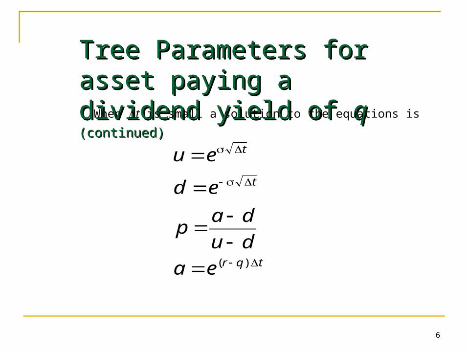
Tree Parameters for Tree Parameters for asset paying a dividend asset paying a dividend yield of yield of q q (continued)(continued)When t is small a solution to the equations is

tqr

t

t

ea

du

dap

ed

eu

)(

7

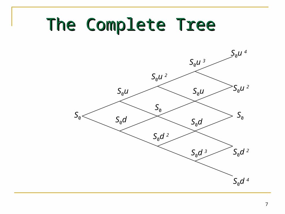
The Complete TreeThe Complete Tree

S0u 2

S0u 4

S0d 2

S0d 4

S0

S0u

S0d

S0 S0

S0u 2

S0d 2

S0u 3

S0u

S0d

S0d 3

8

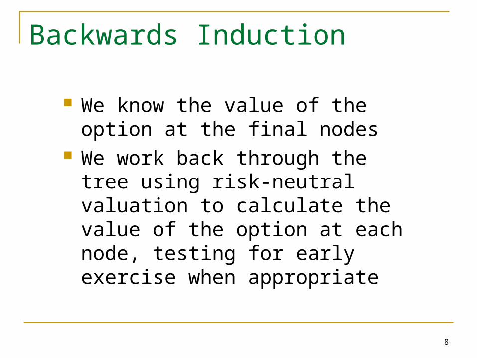
Backwards Induction

We know the value of the option at the final nodes

We work back through the tree using risk-neutral valuation to calculate the value of the option at each node, testing for early exercise when appropriate

9

Example: Put Option

S0 = 50; K = 50; r =10%; = 40%;

T = 5 months = 0.4167;

t = 1 month = 0.0833

The parameters imply

u = 1.1224; d = 0.8909;

a = 1.0084; p = 0.5073

10

Example (continued)

89.070.00

79.350.00

70.70 70.700.00 0.00

62.99 62.990.64 0.00

56.12 56.12 56.122.16 1.30 0.00

50.00 50.00 50.004.49 3.77 2.66

44.55 44.55 44.556.96 6.38 5.45

39.69 39.6910.36 10.31

35.36 35.3614.64 14.64

31.5018.50

28.0721.93

11

Calculation of Delta

Delta is calculated from the nodes at time t

Delta

216 6 96

5612 44 550 41

. .

. ..

12

Calculation of Gamma

Gamma is calculated from the nodes at time 2t

1 2

2

0 64 377

62 99 500 24

377 10 36

50 39 690 64

11650 03

. .

.. ;

. .

..

..Gamma = 1

13

Calculation of Theta

Theta is calculated from the central nodes at times 0 and 2t

Theta = per year

or - . per calendar day

3 77 4 49

016674 3

0 012

. .

..

14

Calculation of Vega

We can proceed as follows Construct a new tree with a volatility of 41%

instead of 40%. Value of option is 4.62 Vega is

4 62 4 49 013. . . per 1% change in volatility

15

Trees for Options on Indices, Currencies and Futures ContractsAs with Black-Scholes:

For options on stock indices, q equals the dividend yield on the index

For options on a foreign currency, q equals the foreign risk-free rate

For options on futures contracts q = r

16

Binomial Tree for Stock Paying Known Dividends

Procedure: Draw the tree for the stock price less the

present value of the dividends Create a new tree by adding the present

value of the dividends at each node This ensures that the tree recombines

and makes assumptions similar to those when the Black-Scholes model is used

17

Extensions of Tree Approach

Other type of trees Time dependent interest rates The control variate technique Path dependent options American options

18

Alternative Binomial Tree

Instead of setting u = 1/d we can set each of the 2 probabilities to 0.5 and

ttqr

ttqr

ed

eu

)2/(

)2/(

2

2

19

Trinomial TreeTrinomial Tree

6

1

212

3

2

6

1

212

/1

2

2

2

2

3

rt

p

p

rt

p

udeu

d

m

u

t

S S

Sd

Su

pu

pm

pd

20

Time Dependent Parameters in a Binomial Tree

Making r or q a function of time does not affect the geometry of the tree. The probabilities on the tree become functions of time.

We can make a function of time by making the lengths of the time steps inversely proportional to the variance rate.

21

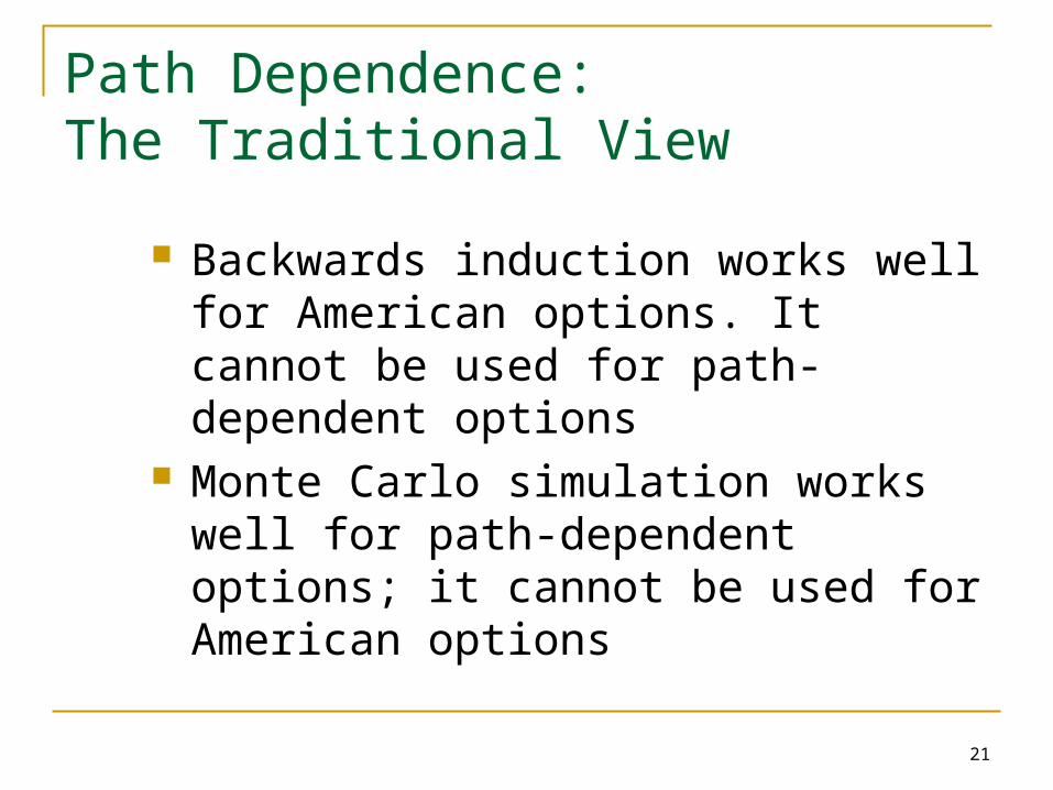
Path Dependence: The Traditional View

Backwards induction works well for American options. It cannot be used for path-dependent options

Monte Carlo simulation works well for path-dependent options; it cannot be used for American options

22

Extension of Backwards Induction

Backwards induction can be used for some path-dependent options

We will first illustrate the methodology using lookback options and then show how it can be used for Asian options

23

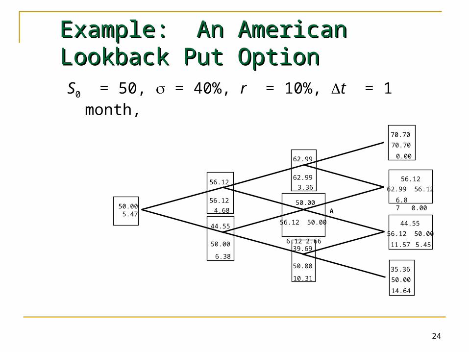
Lookback ExampleLookback Example

Consider an American lookback put on a stock where

S = 50, = 40%, r = 10%, t = 1 month & the life of the option is 3 months

Payoff is Smax−ST We can value the deal by considering all

possible values of the maximum stock price at each node

24

Example: An American Example: An American Lookback Put OptionLookback Put OptionS0 = 50, = 40%, r = 10%, t = 1 month,

56.12

56.12

4.68

44.55

50.00

6.38

62.99

62.99

3.36

50.00

56.12 50.00

6.12 2.66

39.69

50.00

10.31

70.70

70.70

0.00

62.99 56.12

6.87 0.00

56.12

56.12 50.00

11.57 5.45

44.55

35.36

50.00

14.64

50.005.47 A

25

Why the Approach WorksThis approach works for lookback options because The payoff depends on just 1 function of the path

followed by the stock price. (We will refer to this as a “path function”)

The value of the path function at a node can be calculated from the stock price at the node & from the value of the function at the immediately preceding node

The number of different values of the path function at a node does not grow too fast as we increase the number of time steps on the tree

26

Extensions of the Approach The approach can be extended so that

there are no limits on the number of alternative values of the path function at a node

The basic idea is that it is not necessary to consider every possible value of the path function

It is sufficient to consider a relatively small number of representative values of the function at each node

27

Working Forward

First work forward through the tree calculating the max and min values of the “path function” at each node

Next choose representative values of the path function that span the range between the min and the max Simplest approach: choose the min, the

max, and N equally spaced values between the min and max

28

Backwards Induction

We work backwards through the tree in the usual way carrying out calculations for each of the alternative values of the path function that are considered at a node

When we require the value of the derivative at a node for a value of the path function that is not explicitly considered at that node, we use linear or quadratic interpolation

29

Part of Tree to Part of Tree to Calculate Value of an Calculate Value of an Option on the Option on the Arithmetic AverageArithmetic Average

S = 50.00

Average S46.6549.0451.4453.83

Option Price5.6425.9236.2066.492

S = 45.72

Average S43.8846.7549.6152.48

Option Price 3.430 3.750 4.079 4.416

S = 54.68

Average S47.9951.1254.2657.39

Option Price 7.575 8.101 8.635 9.178

X

Y

Z

0.5056

0.4944

S=50, X=50, =40%, r =10%, T=1yr, t=0.05yr. We are at time 4t

30

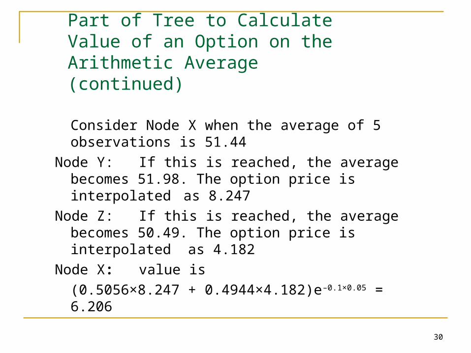
Part of Tree to Calculate Value of an Option on the Arithmetic Average (continued)

Consider Node X when the average of 5 observations is 51.44

Node Y: If this is reached, the average becomes 51.98. The option price is interpolated as 8.247

Node Z: If this is reached, the average becomes 50.49. The option price is interpolated as 4.182

Node X: value is

(0.5056×8.247 + 0.4944×4.182)e–0.1×0.05 = 6.206

31

Using Trees with Using Trees with BarriersBarriers

When trees are used to value options with barriers, convergence tends to be slow

The slow convergence arises from the fact that the barrier is inaccurately specified by the tree

32

True Barrier vs Tree Barrier for a Knockout Option: The Binomial Tree Case

Tree Barrier

True Barrier

33

Inner and Outer Barriers for Inner and Outer Barriers for Trinomial TreeTrinomial Tree

Outer barrierTrue barrier

Inner Barrier

34

Alternative Solutions Alternative Solutions toto Valuing Barrier Valuing Barrier OptionsOptions

Interpolate between value when inner barrier is assumed and value when outer barrier is assumed

Ensure that nodes always lie on the barriers

Use adaptive mesh methodology

In all cases a trinomial tree is preferable to a binomial tree

35

Modeling Two Modeling Two Correlated VariablesCorrelated Variables

APPROACHES:

1.Transform variables so that they are not correlated & build the tree in the transformed variables

2.Take the correlation into account by adjusting the position of the nodes

3.Take the correlation into account by adjusting the probabilities

Monte Carlo Simulation

Why?

36

37

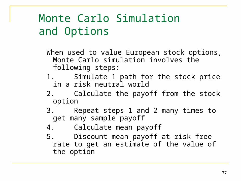
Monte Carlo Simulation and Options

When used to value European stock options,

Monte Carlo simulation involves the following steps:

1.Simulate 1 path for the stock price in a risk neutral world

2.Calculate the payoff from the stock option3.Repeat steps 1 and 2 many times to get many

sample payoff4.Calculate mean payoff5.Discount mean payoff at risk free rate to get an

estimate of the value of the option

38

Sampling Stock Price Sampling Stock Price Movements Movements

In a risk neutral world the process for a stock price is

We can simulate a path by choosing time steps of length t and using the discrete version of this

where is a random sample from (0,1)

tStSS ˆ

dS S dt S dz

39

A More Accurate ApproachA More Accurate Approach

ttetSttS

tttSttS

dzdtSd

or

is this of version discrete The

Use

2/ˆ

2

2

2

)()(

2/ˆ)(ln)(ln

2/ˆln

40

Extensions

When a derivative depends on several underlying variables we can simulate paths for each of them in a risk-neutral world to calculate the values for the derivative

41

Sampling from Normal Sampling from Normal Distribution Distribution

One simple way to obtain a sample

from (0,1) is to generate 12 random numbers between 0.0 & 1.0, take the sum, and subtract 6.0

In Excel =NORMSINV(RAND()) gives a random sample from (0,1)

42

To Obtain 2 Correlated Normal Samples

Obtain independent normal samples x1 and x2 and set

Use a procedure known as Cholesky’s decomposition when samples are required from more than two normal variables

General case

2212

11

1

xxx

43

Standard Errors in Monte Carlo Simulation

The standard error of the estimate of the option price is the standard deviation of the discounted payoffs given by the simulation trials divided by the square root of the number of observations.

44

Application of Monte Carlo Simulation

Monte Carlo simulation can deal with path dependent options, options dependent on several underlying state variables, and options with complex payoffs

It cannot easily deal with American-style options

45

Determining Greek Letters

For 1. Make a small change to asset price2. Carry out the simulation again using the

same random number streams3. Estimate as the change in the option

price divided by the change in the asset price

Proceed in a similar manner for other Greek letters

46

Variance Reduction Techniques

Antithetic variable technique Control variate technique Importance sampling Stratified sampling Moment matching Using quasi-random sequences

47

Sampling Through the Tree

Instead of sampling from the stochastic process we can sample paths randomly through a binomial or trinomial tree to value a derivative

48

Monte Carlo Simulation and American Options

Two approaches: The least squares approach The exercise boundary parameterization

approach Consider a 3-year put option where the initial

asset price is 1.00, the strike price is 1.10, the risk-free rate is 6%, and there is no income

49

Sampled Paths

Path t = 0 t =1 t =2 t =3

1 1.00 1.09 1.08 1.34

2 1.00 1.16 1.26 1.54

3 1.00 1.22 1.07 1.03

4 1.00 0.93 0.97 0.92

5 1.00 1.11 1.56 1.52

6 1.00 0.76 0.77 0.90

7 1.00 0.92 0.84 1.01

8 1.00 0.88 1.22 1.34

50

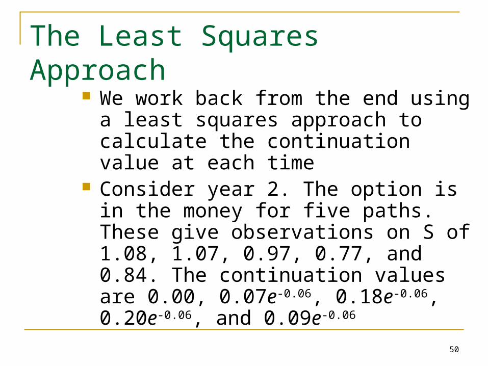
The Least Squares Approach

We work back from the end using a least squares approach to calculate the continuation value at each time

Consider year 2. The option is in the money for five paths. These give observations on S of 1.08, 1.07, 0.97, 0.77, and 0.84. The continuation values are 0.00, 0.07e-0.06, 0.18e-0.06, 0.20e-0.06, and 0.09e-0.06

51

The Least Squares Approach continued

Fitting a model of the form V=a+bS+cS2 we get a best fit relation

V=-1.070+2.983S-1.813S2

for the continuation value V This defines the early exercise decision

at

t =2. We carry out a similar analysis at t=1

52

The Least Squares Approach continued

In practice more complex functional forms can be used for the continuation value and many more paths are sampled

53

The Early Exercise Boundary Parametrization Approach We assume that the early exercise boundary can

be parameterized in some way We carry out a first Monte Carlo simulation and

work back from the end calculating the optimal parameter values

We then discard the paths from the first Monte Carlo simulation and carry out a new Monte Carlo simulation using the early exercise boundary defined by the parameter values.

54

Application to Example

We parameterize the early exercise boundary by specifying a critical asset price, S*, below which the option is exercised.

At t =1 the optimal S* for the eight paths is 0.88. At t =2 the optimal S* is 0.84

In practice we would use many more paths to calculate the S*

55

Finite Difference Methods

Finite difference methods aim to represent the differential equation in the form of a difference equation

We form a grid by considering equally spaced time values and stock price values

Define ƒi,j as the value of ƒ at time it when the stock price is jS

56

Finite Difference Methods(continued)

or

set we

In

2

11

2

2

11

2

2

11

2

222

2

2

2

1

SΔ

ƒƒƒ

S

ƒ

SΔSΔ

ƒƒ

SΔ

ƒƒ

S

ƒ

ΔS

ƒƒ

S

ƒ

rƒS

ƒSσ

S

ƒrS

t

ƒ

i,ji,ji,j

i,ji,ji,ji,j

i,ji,j

57

Implicit Finite Difference Implicit Finite Difference MethodMethod

:form the of

equations ussimultaneo solving involves This

method. difference finite implicit the obtain we

set also weIf

ƒƒcƒbƒa

tΔ

ƒƒ

t

ƒ

,jii,jji,jji,jj

i,j,ji

111

1

58

Explicit Finite DifferenceExplicit Finite Difference

ƒcƒbƒaƒ

ji,j,i

SfSf

,ji*j,ji

*j,ji

*ji,j 11111

2

1

:form the of equations solving involves This

method difference finite explicit the obtain we

point )( the at arethey as point )( the at

same the be to assumed are and If 2

59

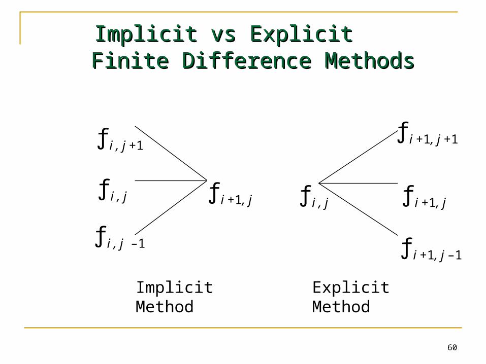
Implicit vs Explicit Finite Difference Method

The explicit finite difference method is equivalent to the trinomial tree approach

The implicit finite difference method is equivalent to a multinomial tree approach

60

Implicit vs ExplicitImplicit vs Explicit Finite Difference Methods Finite Difference Methods

ƒi , j ƒi +1, j

ƒi +1, j –1

ƒi +1, j +1

ƒi +1, jƒi , j

ƒi , j –1

ƒi , j +1

Implicit Method

Explicit Method

61

Other Points on Finite Difference Methods

It is better to have ln S rather than S as the underlying variable

Improvements over the basic implicit and explicit methods: Hopscotch method Crank-Nicolson method

Comparison of different methods

62