1 Module Ten: Planning Experiments – the general consideration and Comparative Study for more than two groups For any quantitative investigation, it usually

1

Module Ten:

Planning Experiments – the general consideration and

Comparative Study for more than two groups

For any quantitative investigation, it usually involves a variety of steps before the data is ready for analysis. It is crucial that the data for the final analysis is valid and reliable. Therefore, a scientific process for producing valid and reliable data is extremely important. Data are usually collected from either surveys or experiments. The type of studies can be loosely classified in terms of observational study and experimental study. In the first section of this module, we will discuss some general considerations of conducting an appropriate experimental study.

2

DO THE RIGHT THING!

(Planning and designing appropriate experiment)

DO THE THINGS RIGHT!

(collecting appropriate data and conducting appropriate analysis)

To plan an experimental study, here is a list of considerations that should be taken into account:

•Determine the specific objective of the experiment.

•Determine the response variables and the ways of measuring these measurements.

•Identify factors that are potentially influential to the response measurements.

•Determine which factors to vary and controlled in the experiment and which to be held at constant or it’s influence should be minimized.

•Determine the specific design and procedure for conducting the experiment.

•Determine the number of replications of the basic experiment to conduct.

•Identify and secure available resources, material and facility needed.

3

A few terms used in design of experiments

Treatments: As et of circumstances created for the experiment in response to the purpose of the study. Some times, the term factors are also used when there are more than one factor. Each factor may have two or more factor levels. For example, if we have two factors, temperature and type of material. Three levels of temperature and four types of material will be planned for the experiment. We have an factorial design with two-factors, and the total # of treatment combinations = 3x4 = 12 treatment combinations.

Experimental unit: the physical entity or subject that are exposed to the treatment.

Experimental error: describe variation among the identical and independently treated experimental units. The potential sources of variability may come from:

1. The nature variation among experimental units

2. Variability in measurement of response

3. Inability to reproduce the treatment condition exactly from one unit to the other.

4. Interaction of treatments or experimental units

5. Any other external factors that may influence the measured characteristic.

4

The experimental design techniques are implemented to answer the purpose of the study, usually involves with the investigation of some hypothesis of interest as valid and reliable as possible. That is, in any experiment, we should try to minimize the systematic bias and reduce the experimental error.

For example: here are some possible designs for designing the 3x4 (temperature, material) factorial experiment:

1. Prepare 12 experiment units, and randomly assign one unit to each treatment combination. In this assignment, there is no replication for each combination This is a 3x4 factorial design without replication. It is a completely randomoized design set up.

2. A possible design is to have two replications for each treatment combination. In order to achieve this, we will need a total of 24 experimental units. Two units are randomly assigned to each treatment combination. This is a 3x4 factorial design with 2 replications.

3. Another possible design: Factorial with Block design. In many experiments, there environmental limitations such as location, or time. Suppose there are two labs that will be conducting this experiment. Design (2) does not take this external factor into account. It is possible that each lab has different systematic error. Design two may ends up to assign A and B material, but little or no C and D material in the randomization process. This will cause a problem we call:

5

Confounding: The effect between material (A,B) and (C,D) is mixed with the Lab difference. We have no way to separate these two effects unless we can assume there is very systematic error between two labs.

One way to deal with this problem is to introducing Blocking factor. Take each lab as a block. Then, apply a completely randomized design within each Block. In the 3x4 factorial experiment, we randomly select 12 experimental units, randomly assign one to each treatment combination. And repeat the same procedure for Lab two.

Through ‘Blocking’ control, we will be able to separate the Lab effect.

4. One can conduct a 3x4 factorial with 2 replications for each lab. In this design, we can also estimate within-lab variability as well as between lab variability along with all treatment effects. However the total number of experimental units will be 3x4x2x2 = 48

6

5. There is yet another important consideration for the 3x4 factorial experiment. Within the same lab, it is possible that there is a day-to-day systematic error. If such a systematic error is huge, it means the results obtained on Monday may be significantly different from that obtained on Tuesday. The consequence is that any uncertainty measurement is time-dependent. That is not appropriate. Therefore, one can conduct an experiment to study if day-to-day variability is a concern. To plan such an experiment, we will need to repeat the same 12 treatment combinations on some randomly selected days, say three, within the time period of the experiment.

This design involves factorial experiments conducted in two labs, and the randomly selected tree days are nested within each lab.

6. There are other types of designs developed for some specific purposes. For example, fractional factorial design is usually applied to situations where we have a huge number of treatment combinations, and it takes either two much money or two much time, or the physical environment can not implement a complete experiment. As a consequence, we may plan half or even quarter of the complete factorial design. By doing so, we will not able to estimate all possible effects. Fortunately, there are some statistical and practical principles that help us to choose designs that will only sacrifice the effects that may not be significant or may not be as important. For example, if we have 8 factors, two levels for each factor. We have 28 treatment combinations. To conduct a complete factorial experiment without replication, we will need 256 experiment units. If we can conduct one quarter experiment runs (64), we still have 64 data for us to investigate and identify important factors and some interactions effects, if we plan and implement some appropriate fractional designs.

7

For the first part of the discussion, I will focus on important analysis tools that can be applied to every type of designs. The completely randomized design with one-factor will be used as the basis for this discussion.

In the previous module, we discuss how to analyze a factor with two levels. We introduce paired sample and independent sample. In this section, we extend the two group independent sample to more than two groups. This is what we usually named as one-way ANOVA technique.

Paired sample is extended using the concept of ‘Blocking’ in the general set up.

8

Local Control of Experimental Errors

In conducting an experiment, we would like to be able to make a precise and accurate comparison among treatments over a proper range of conditions. Some local control is possible for reduce or control experimental error, increase the accuracy of the observations and make valid inference for the study.

The experimenters can control:

1. Techniques – including tasks such as preparation of material, lab facility, calibration of instruments, design techniques that meet the purpose of the investigation.

2. Selection of uniform experimental units – The selection of experimental units should take into account the regular condition that encountered in the field not just try to unify the unit. For example, it is not a good idea to take consecutive units from the process for experiment, since they are dependent.

9

3. Blocking to reduce experimental error variation,

4. Recording possible covariates. In many experiments, the response variables may be affected by some other variables of the same experiment unit. These variables will also undergoing changes during the experiment and they may have direct effect to the response. For example, when studying how different amount of a chemical component affect the brightness of paper, for each paper we measure the brightness, it would be important to also measure the roughness of the paper, since the roughness of the paper also have a direct effect on the brightness. The variable, Roughness is a covariate.

5. Replications: If a treatment is applied to only one unit, we will not be able to estimate the experimental error, nor can we know if the results can be reproduced. Replications allow us to

• Demonstrate if the results can be reproduced or not,

• Estimate the experimental error,

• Increase the precision of the estimate.

The size of replication depends on (a) overall variance, (b) the size of anticipated difference between two means, © Type I error and (d) Power of test = 1- type II error. Minitab has a set of procedures for this, which will not be discussed here.

10

Why Randomization?

In the choice of experimental units and the assignment of the units to treatment, we emphasize the use of ‘randomization’.

The importance of ‘randomization’ include”

1. Random selection of experimental units makes the statistical assumption of independent valid. When two units are chosen at random, it implies what ever we will measure from the second unit is not dependent on the choice of the first unit. This is easy to understand in any survey study.

2. Random assignment of units to treatment balances the possible bias due to the units, in to prevent potential confounding effects.

11

In laboratory studies, it is often that more than two groups are to be compared. This is an extension of two-sample comparative study.

• A typical technique for analyzing comparing more than two groups is the Analysis of Variance.

• For most of comparative studies for more than two groups, the ANOVA is the first step of the analysis. ANOVA tells us if there is an overall differences among group means. AN important question after the ANOVA is to ask which group is different from which group, or if there is any identifiable pattern or trend when comparing these group means.

• For the rest of this Module, we will discuss

1. the concept behind ANOVA, how to conduct ANOVA,

2. how to perform post-hoc analysis,

3. how to set up contrasts,

4. how to identify patterns and test the significance of the existing patterns or trends.

12

Consider a laboratory study to compare the compressive strength of hydraulic cement mortars.

A study is conducted to compare the compressive strength (psi) on five different sizes of sands by using five different screens of diameters: 200 m, 400 m, 600 m, 800 m, 1000 m.

Purpose: To compare the compressive strength of concrete made of five sizes of sands, and to identify the size of sand that will result maximum compressive strength.

Design: Five sizes of sands are prepared based on the above five screen sizes. For each size of sand, 12 samples will be randomly chosen for producing specimen which will be tested. Eight ‘good’ specimen will be selected for strength testing.

Experiment: A commonly used process and formula will be applied for the experiment. The compressive strength test will be conducted four weeks after the specimen was formed. The same testing procedure will be applied to every specimen.

Measurement: The standard psi readings will be recorded along with any unusual incidents during the experiment or testing process.

13

The strength data are given in the following table(in 100 psi)

Size (max) 1 2 3 4 5 6 7 8

200m 34.5 25.6 31.3 24.9 28.0 29.4 32.8 30.4 29.61 3.35

400m 48.6 52.6 63.9 62.5 58.3 53.8 54.0 61.5 56.90 5.46

600m 57.5 59.6 48.4 56.2 53.8 52.2 47.3 45.2 52.53 5.18

800m 50.3 45.8 42.7 44.8 41.7 45.8 38.4 39.2 43.59 3.91

1000m 22.0 25.2 27.4 23.8 21.7 19.6 21.5 19.4 22.58 2.75

iy is

Questions to ask:

1. Are the mean strengths significantly different?

2. What sand size will produce the maximum strength?

3. If there is a significant difference among the five sand sizes, which one is different from which one?

4. What kind of relationship between strength and sand size can be identified?

5. In conducting the analysis we also need to conduct diagnosis of the assumptions: Normality and constant variance.

6. What should we do if the an assumption is seriously violated?

14

Statistical Model for One-Way ANOVA

An appropriate analysis and interpretation is based on an underlying statistical model to describe the response variable, y. For the concrete strength data, y is the compressive strength.

•For this case, each y observation is labeled by the sand size and the specimen within the sand type by the notation, yij , representing the ith sand size and the jth specimen within the sand size.

•For each specimen, there is a true unknown mean, denoted by

•The deviation: yij – i is the random error, denoted by ij, which is assumed to follow a normal distribution with mean 0 and s.d., .

Therefore, the statistical model describes this one factor experiment is:, 1,2, groups; j = 1,2, , r replications.

where is the random error with mean 0 and s.d., ,

and is usually assumed to be follow a normal curve.

This is the Cell Mean model. 's ari

ij i ij

ij

y i t

e the unknown

treatment (or group) means.

15

A quick check of the treatment means and within-treatment variation, the distribution for each treatment level is illustrated in the figure:

Note that: a quick eye-check indicates that the distribution of the population for each treatment level may have different mean and different variation based on the sample data. The order of the unknown treatment means is estimated by using the sample means, and the shape is assumed normal with different variations, based on the sample s.d.

•Since a typical ANOVA requires normality and equal variance, the process of the analysis should also include the diagnosis of the assumptions

•If the assumption(s) is violated, some actions should be taken before performing ANOVA table and other analysis.

•Common approaches for taking care of the violation of assumptions include

•Data transformation,

•Use techniques that are more robust to these assumptions, such as nonparametric techniques.

16

An alternative model that provides better interpretation of ANOVA is the Treatment Effect Model, which has the form:

yij = it ; j = 1,2,…, r.

The components in the model:

is the grand mean. i is the ith treatment effect = –

ij is the random error , which is independently distributed with mean 0 and s.d. Each of these components is estimated by the corresponding sample data:

i ij i

i

i i

.. ... .) ( )

e , i = 1,2,..., t ; j = 1,2, ..., r .

When replicatrions are equal, r for all i.

Total number of observations: N = r (when all r is a

(

= ˆ ˆij i ij i

r

tr

y y y y y y

t

i=1

1 1

i. ij1

..

re equal)

( ) / , the grand mean of all observations.

y ( y ) /

NOTE: The estimates are obtained by using the Least Square Method.

i

i

rt

iji jr

ij

y N

r

y

17

Treatment Specimen Observation yij Cell Mean Model Effect Model

200 1 34.5 y11

200 2 25.6 y12

…… …... …… …..

200 8 30.4 y18

400 1 48.6 y21

400 2 52.6 y22

….. ---- …… ------

---- ----- …… ------

1000 1 22.0 y51

1000 2 25.2 y52

------ ------ …… ……

1000 8 19.4 y58

Size (max) 1 2 3 4 5 6 7 8

200m 34.5 25.6 31.3 24.9 28.0 29.4 32.8 30.4 29.61 3.35

400m 48.6 52.6 63.9 62.5 58.3 53.8 54.0 61.5 56.90 5.46

600m 57.5 59.6 48.4 56.2 53.8 52.2 47.3 45.2 52.53 5.18

800m 50.3 45.8 42.7 44.8 41.7 45.8 38.4 39.2 43.59 3.91

1000m 22.0 25.2 27.4 23.8 21.7 19.6 21.5 19.4 22.58 2.75

iy is

18

The Sum of Square Decomposition provides the basis of the ANOVA Table:

2 2 2

.. . .. ..( ) ( ) ( )

SS Total = SS Treatment + SS Error

SSTO = SSTR +

ij i ijy y y y y y

SSE

Total SS = Between-Group SS + Within-Group SS

_______________________________________________________

Total D.F. = D.F. Due to Treatment + D.F. Due to Error

(N-1) = (t-1) + (N-t)

NOTE: The Within-Group S.S. is the sum of the weighted within-group variances:

The assumption of constant variance allows

2

SSE is the combined Sum of Square due to error, hence, the estimated variance can be determined

Dividing SSE by its D.F. : S /( )

us to estimate the common variance using the entire data.

SSE N t t, which is the MSE in he ANOVA table

19

The following model is a full model, in the sense that it covers the situation that the group means are different.

yij = it ; j = 1,2,…, r.

is the grand mean. i is the ith treatment effect = –

ij is the random error , which is independently distributed with mean 0 and s.d.

One of our purpose is to test if indeed the groups have different means. That is we are interested in testing a hypothesis:

0 1 2

0 1 2

: Vs. : Not all 's are all equal

Similarly, if we use the effects model, the hypothesis is

: 0 Vs. : Not all 's are all equal to zero.

t a i

t a i

H H

H H

The full model above represents the situation when Ha occurs.

When H0 occurs, the model is reduced to

yij = ij

This is usually called a reduced model.

20

Reduced Model Full Model

Treatment Specimen Observation Estimate Difference Estimate Difference

200 1 34.5 41.04

200 2 25.6 41.04 29.61 -4.01

…… …... …… …..

200 8 30.4 41.04 29.61

400 1 48.6 41.04 56.90 -8.30

400 2 52.6 41.04 56.90 -4.30

….. ---- …… ------

---- ----- …… ------

1000 1 22.0

1000 2 25.2

------ ------ …… ……

1000 8 19.4

The observed values, estimates,and deviations using full and reduced models are illustrated in the following table:

To be completed as a hands-on activity

21

A graphical presentation of the least square estimates of components in the model

20

0

40

0

60

0

80

0

10

00

20

30

40

50

60

Sand Size

Str

eng

thDotplots of Compressive Strength by Sand-Size

41.04

29.61

56.9052.53

43.59

22.58

22

ANOVA Table for One-Way Analysis

Source of Variation Degrees of Freedom

Sum of Squares

Mean Square F-value P-value

Treatment (Between Group)

t – 1 SSTR MSt = SSTR/(t-1) MSt/MSE P(F > F-value)

Error

(Within Group)

N - t SSE MSE=SSE/(N-t)

Total N - 1 SSTO

NOTE:

(1) SSTO = SSTR + SSE

(2) (2) DF Total = DF Treatment + DF Error

(3) F-test tests the hypothesis:

(4) The decision rule based on the p-value:

If p-value < , then, we conclude Ha: Not all group means are equal.

0 1 2: Vs. : Not all 's are all equalt a iH H

23

Why the F-test can be used to test the hypothesis?

One way to understand why F-test does the job we ask for is to find out the Expected Values of MSE, MSt and look at the ratio of MSt/MSE in terms of the expected values.

This can be done by hand. The modern computer technology and statistical software can actually provide the expected value of MSE and MSt. All we need to understand is about the ratio and the relationship of the ratio with F-test.

For One-factor design, the following gives the needed expected values:2

22 2 2

i

22 2

i

( )

( ) . When replications are equal to r, ( ) 1 1

The F-value = MSt/MSE tells us how large / is , which is deptermined by the .1

This is the squared tr

i i

i i

E MSE

r rE Mst E Mst

t t

r

t

eatment effect for the ith group. The larger the differences among group

means, the larger the F-value will be. Under the assumption that the samples are selected

at random from normal populations, the F-distribution can be applied to conduct an

appropriate test.

24

Analysis of the Compressive Strength of concrete made by five sand sizes

Procedure of the analysis:

1. Preparing the data: data cleaning to make sure no known errors due to sampling or other special causes.

2. Perform descriptive analysis using graphical and numerical tools.

3. Checking outliers.

4. Conduct appropriate analysis of variance., and conduct residual analysis to check if the assumptions of normality and constant variance are appropriate. If yes, go to step 5; otherwise, take proper steps to adjust data and repeat this step.

5. If the F-test shows significant, it says there exists significant differences among treatment means, go to step 6; otherwise, go to step 7.

6. Conduct appropriate multiple comparison procedures to reveal which treatment is different from which treatment or conduct trend analysis to investigate the trend/patterns between the response and the treatments.

7. Summarize and report the results in the context of the problem.

25

Size (max) 1 2 3 4 5 6 7 8

200m 34.5 25.6 31.3 24.9 28.0 29.4 32.8 30.4 29.61 3.35

400m 48.6 52.6 63.9 62.5 58.3 53.8 54.0 61.5 56.90 5.46

600m 57.5 59.6 48.4 56.2 53.8 52.2 47.3 45.2 52.53 5.18

800m 50.3 45.8 42.7 44.8 41.7 45.8 38.4 39.2 43.59 3.91

1000m 22.0 25.2 27.4 23.8 21.7 19.6 21.5 19.4 22.58 2.75

iy is

Variable Sand Size N Mean Median TrMean StDev

Strength 200 8 29.61 29.90 29.61 3.35

400 8 56.90 56.15 56.90 5.46

600 8 52.53 53.00 52.53 5.18

800 8 43.59 43.75 43.59 3.91

1000 8 22.575 21.850 22.575 2.748

Variable Sand Size SE Mean Minimum Maximum Q1 Q3

Strength 200 1.18 24.90 34.50 26.20 32.42

400 1.93 48.60 63.90 52.90 62.25

600 1.83 45.20 59.60 47.58 57.18

800 1.38 38.40 50.30 39.83 45.80

1000 0.972 19.40 27.400 20.075 24.85

26

20

0

40

0

60

0

80

0

10

00

20

30

40

50

60

Sand Size

Str

engt

h

Boxplots of Compressive Strength of Concrete by Sand Size

10

00

80

0

60

0

40

0

20

0

60

50

40

30

20

Sand Size

Str

eng

thDotplots of Compressive Strength by Sand-Size

41.04

29.61

56.9052.53

43.59

22.58

A quick check indicates:

1. Group means are very different with size = 400 the maximum.

2. Does not seem to have outliers

3. Constant variance may not hold.

4. Normality looks okay.

270 5 10 15

95% Confidence Intervals for Sigmas

Bartlett's Test

Test Statistic: 4.248

P-Value : 0.373

Levene's Test

Test Statistic: 2.059

P-Value : 0.107

Factor Levels

200

400

600

800

1000

Test for Equal Variances for Strength20 30 40 50 60

-10

-5

0

5

Fitted Value

Res

idua

l

Residuals Versus the Fitted Values(response is Strength)

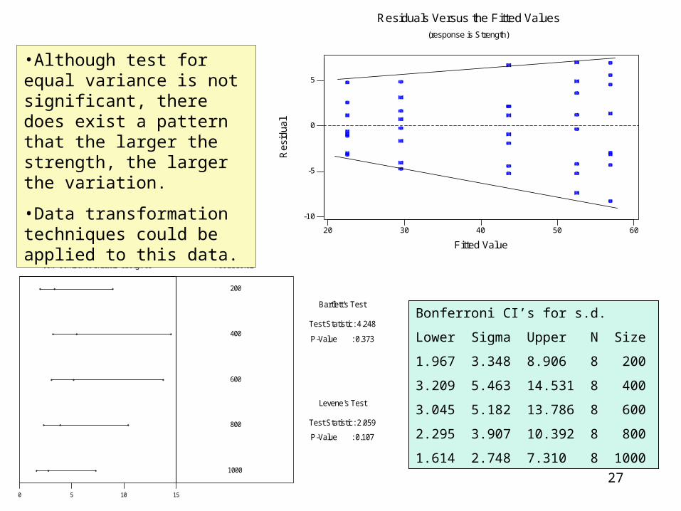
•Although test for equal variance is not significant, there does exist a pattern that the larger the strength, the larger the variation.

•Data transformation techniques could be applied to this data.

Bonferroni CI’s for s.d.

Lower Sigma Upper N Size

1.967 3.348 8.906 8 200

3.209 5.463 14.531 8 400

3.045 5.182 13.786 8 600

2.295 3.907 10.392 8 800

1.614 2.748 7.310 8 1000

28

Data Transformation for adjusting the violation of assumptions

Two important assumptions are required in ANOVA:

1. Population where we observe data should be approximately normal.

2. The within-group variances should be approximately equal.

We apply outlier detection technique, normality test and homogeneity of variance test to conduct the diagnosis.

For the Strength data, the diagnosis shows no serious violation of these assumptions. Therefore, the ANOVA results are appropriate, and we can conduct multiple comparisons or trend analysis.

However, the plot of residuals Vs. estimated response values does show a clear pattern that when the strength is larger, the variance is larger. That is there is a relation linear positive relation between variances and group means:

d

, that is

If we take a power transformation of the data: w = y , we hope to achieve the result that

does not depend on . This is achieved by examing the relatioship between and

b by y

w w w

a

1

:

After the transformation, the relationship between and is approximated by

Therfore, if we let d = 1-b, then, no longer depends on .This suggests if we can est

w

d bw

w

imate the power b,

we can obtain a good power transformation so that the new variable, w, will give us constant variance.

29

Data Transformation – Continued:

How to estimate b so that d can be determined by d = 1-b

A quick and easy approach is to fit a simple linear regression line:

i

log( ) log( ) log( )

By using the sample data, we fit the simple regression line:

log(s ) log( ) log( )

i i

i

a b

a b y

Some commonly applied power transformations are

d = 1-b yd Name Explanation

2 y2 Square Also transform skewed-to left distribution to close to normal

1 Y No transformation

½ Square Root When Y follows Poisson distribution, this will transform Y to close to normal.

0 Ln(y) Ln transformation Also transform skewed-to-right distribution to close to normal. (If y = 0, add .25 or .5 to the every observation.)

-1/2 1/ Reciprocal square root

-1 1/y Reciprocal Reexpress time to rate.

y

y

30

29.61 3.35

56.90 5.46

52.53 5.18

43.59 3.91

22.58 2.75

iy is The fitted simple regression line is:

3.0 3.5 4.0

1.0

1.1

1.2

1.3

1.4

1.5

1.6

1.7

ln(ybar)

ln(s

d)

ln(sd) = -1.251 + 0.72 ln(ybar)S = 0.0701710 R-Sq = 95.6 % R-Sq(adj) = 94.1 %

For the Compressive Strength data, we have

Therefore, an appropriate transformation is d = 1-b = 1-.72 = .28 which suggests we may apply a log transformation or a square root transformation. In the following we use the Ln transformation to re-analyze data, and compare if the results are similar or not.

31

General Linear Model: Strength versus Sand Size

Factor Type Levels Values

Sand Size fixed 5 200 400 600 800 1000

Analysis of Variance for Strength, using Adjusted SS for Tests

Source DF Seq SS Adj SS Adj MS F P

Sand Size 4 6891.8 6891.8 1723.0 94.96 0.000

Error 35 635.0 635.0 18.1

Total 39 7526.9

Unusual Observations for Strength

Obs Strength Fit SE Fit Residual St Resid

9 48.6000 56.9000 1.5060 -8.3000 -2.08R

R denotes an observation with a large standardized residual.

ANOVA Table indicates the treatment means are significantly different (p-value of the F-test = .000).

An unusual observation is located with standardized residual = -2.08. This is, however,, not a serious problem. Besides, there is no special causes for this observation. It should be kept for the entire analysis.

32

Expected Mean Squares, using Adjusted SS

Source Expected Mean Square for Each Term

1 Sand Size (2) + Q[1]

2 Error (2)

Error Terms for Tests, using Adjusted SS

Source Error DF Error MS Synthesis of Error MS

1 Sand Size 35.00 18.1 (2)

Variance Components, using Adjusted SS

Source Estimated Value

Error 18.14

the variance for Error Term , is named as the source (2)

Q[1] is the Quadratic fixed quantity due to Sand Size, the Source (1), which is

This tells us what/how we should perform the F-test.

2

1i ir

t

The source (1), Sand Size is tested by the Source (2). The DF of the Source (2) is 35, and the Mean Square for the Source (2) is 18.1.

This performs all F-tests that are meaningful and appropriate for the analysis.

In this one-way model, the only component that is purely about variation is the random error variance. It is estimated by the MS Error.

33

Least Squares Means for Strength

Sand Size Mean SE Mean

200 29.61 1.506

400 56.90 1.506

600 52.53 1.506

800 43.59 1.506

1000 22.58 1.506

•The final part of the results is the Least Square estimates of group mean for each Sand Size and the corresponding SE of each group mean.

•SE Mean measures the uncertainty of the estimated group mean.

•The Least Square Mean is the same as the sample mean of each Sand Size, when the replications are all equal, which is the case for this study, r = 8.

•The SE Mean is the estimated population s.d. divided by the square root of the number of observations that are used to compute the group mean.

The estimated common population variance is MSE, and each Least Square Mean is the mean of r = 8 strengths. Therefore, SE Mean is given by

/MSE r

/ 18.14 / 8MSE r

34 200 400 600 800 1000

25

35

45

55

Sand Size

Str

eng

th

Main Effects Plot - LS Means for StrengthAverage: 0.0000000StDev: 4.03525N: 40

Anderson-Darling Normality TestA-Squared: 0.271P-Value: 0.657

-5 0 5

.001

.01

.05

.20

.50

.80

.95

.99

.999

Pro

babi

lity

RESI1

Normal Probability Plot of the Residuals

The main effect plot shows there is a nonlinear relationship between Strength and Sand Size.

The Normality test of the residuals shows no violation of normality assumption.

35

Analysis of the Ln-Transformed Strength Data

General Linear Model: LnStrength versus Sand size


Sand size fixed 5 200 400 600 800 1000

Analysis of Variance for LnStreng, using Adjusted SS for Tests


Sand size 4 4.9715 4.9715 1.2429 113.80 0.000

Error 35 0.3822 0.3822 0.0109

Total 39 5.3537

Unusual Observations for LnStreng

Obs LnStreng Fit SE Fit Residual St Resid

35 3.31054 3.11054 0.03695 0.20001 2.05R

R denotes an observation with a large standardized residual.

NOTE: The ANOVA results are similar to the raw data. Therefore, it is recommended that we should focus on the raw data, since the values are meaningful and easier to interpret.

36

3.0 3.5 4.0

-0.2

-0.1

0.0

0.1

0.2

Fitted Value

Res

idua

lResiduals Versus the Fitted Values

(response is Ln(Strength))

Average: 0.0000000StDev: 0.0990005N: 40

Anderson-Darling Normality TestA-Squared: 0.346P-Value: 0.466

-0.1 0.0 0.1 0.2

.001

.01

.05

.20

.50

.80

.95

.99

.999

Pro

babi

lity

RESI-LN

Normal Probability Plot of the Residuals for theLN(Strength) Response Variable

The plot of Residual Vs. Fitted Value show the within-group variances are approximately the same. It is somewhat better than the raw data. The analysis results have little different. Therefore, due to the difficulty of interpreting the results, one should focus on the analysis of the raw data for this case.

The normal probability plot is almost the same as the result using the raw data.

37

Post Hoc analysis after the ANOVA

According to the ANOVA results, we conclude that the strengths of difference sand sizes are significantly different. But, we would like to take one more step to find out which one is different from which one. This is a post-hoc comparison.

Several post-hoc comparisons have been developed. Each one has its purpose. In this section, we will introduce the following types of comparisons:

1. Specific comparisons of interest – Contrasts

2. Trend analysis when the treatment levels are ordinal scales

3. Simultaneous multiple comparisons:

• Bonferroni simultaneous confidence interval

• Comparisons with a control – Dunnette’s method

• Pair-wise comparison : the Tukey’s method

38

Planning comparisons among Treatments - Contrasts

Contrast allows us to make any treatment comparison of interest.

For the Concrete Strength case, suppose we suspect that very small and very large sand sizes may result very different strength from the middle sand size. We can then set up a specific comparison for this purpose by comparing the mean of Sand Size 200 and 1000 with the mean of Sand Size 600. In terms of the notation used for population means, this is equivalent to testing the hypothesis:

Parameter

Coefficient ½ 0 -1 0 ½

Notation for coefficient c1 c2 c3 c4 c5

1 5 1 50 3 3

1 5 1 50 3 3

: Vs. :2 2

Equivalently, this hypothesis can be written as

: =0 Vs. : 02 2

a

a

H H

H H

The coefficients associated with the population means are:

39

Note: the sum of ci’s = 0: (1/ 2) 0 ( 1) 0 (1/ 2) 0ic We call the following a contrast among the treatment means:

with the property: c 0i i iC c 1 5

3

2 3 4 5

1 3 4

is a contrast.2

is a contrast

3 4 is a contrast

Examples:

Hands-on activity: Define two contrasts of interest for the concrete example. Are these two contrasts orthogonal?

In many situations, we are interested in more than two contrasts. It is important to learn the relationship between two contrasts. When two contrasts have the following relationship, we say two contrasts are orthogonal

and are two contrasts.

If 0, then contrasts C and D are orthogonal.

i i i i

i i

C c D d

c d

40

How to conduct a hypothesis test:

How to construct a confidence interval for the contrast:

0 : 0 Vs. : 0i i a i iH c H c i ic

The purpose of forming a contrast is either for testing a hypothesis or constructing a confidence interval to estimate the expanded uncertainty.

t

A common and general technique for testing a hypothesis or constructing a confidence interval for any contrast is:

1. Obtain the sample estimate of the contrast:

2. Determine and obtain the measurement uncertainty of

For this case, it is SE of , which is

3. For hypothesis test, compute t-value:

4. 100(1-)% C.I. for is

.i ic y.i ic y

.i ic y2

2. i( ) ( ) ( ) if replications, r 's all equal to r.i

i i ii

c MSESE c y MSE c

r r

.

.( )i i

i i

c yt

SE c y

i ic

. ( / 2, ) .( )i i N t i ic y t SE c y

41

Construct a 95% confidence interval for the contrast

And test the hypothesis:

1 532

1 5 1 50 3 3: =0 Vs. : 0

2 2aH H

Size (max) replication

200m 8 29.61

400m 8 56.90

600m 8 52.53

800m 8 43.59

1000m 8 22.58

iy From ANOVA table,

MSE = 18.1 and DF = 35

The Least Square Estimate of is

= (29.61+22.58)/2 – 52.53 = -26.435

SE( ) =

1 532

1 5 3( ) / 2y y y

1 5 3( ) / 2y y y 2 18.1(.25 0 1 0 .25) 1.842

8i

MSEc

r

95% CI is

95% of chance that the true difference between mean strength of sand size 600 and Sand Sizes (200, 1000) is from 2270 psi to 3018 psi.

(.025, ) 26.44 2.03(1.842) [ 30.18, 22.70]N t CC t SE

42

To test the hypothesis:

Using t-test:

P-value is 2P(t > |tobs|) = 2P(t > 14.35) =.000

We conclude the mean strength of sand sizes (200, 1000) is significantly different from the strength of size 600. Indeed, Size 600 results significantly higher strength.

1 5 1 50 3 3: =0 Vs. : 0

2 2aH H

26.4414.35

1.842obsC

Ct

SE

Hands-on Activity

1. Obtain a 90% confidence interval for the contrast , C, you set up. Interpret your confidence interval.

2. Test the hypothesis : H0: C = 0 Vs. Ha: , and interpret your result.

0C

43

A Sum of Squares Decomposition for a Contrast

A contrast consists of one degree of freedom information. In the terminology of Sum of Square, it is part of the sum of squares from the treatment effect.

Sum of Squares Due to the contrast C = can be computed from the least square means:

For the contrast, of the concrete strength example,

The Sum of Square of this one d.f. contrast is

SSC = 8 (-26.44)2/(.25+0+1+0+.25) = 3728.39

i ic 2 2

i2 2 , if r are equal.

( / )

i i i i

i i i

c y c ySSC r

c r c

1 532

Hands-on Activity

Compute the SSC for the two contrasts that you set up for this concrete strength example

44



Sand Size 4 6891.8 6891.8 1723.0 94.96 0.000

(1,5) Vs 3 1 3728.4 3728.4 3728.4 205.99 0.000

Rest 3 3163.4 3163.4 1054.5 58.26 0.000

Error 35 635.0 635.0 18.1

Total 39 7526.9

ANOVA Table with Sum of Squares Decomposition

NOTE:

•We can test a contrast using t-test, as presented before. We can also test a contrast using F-test, and include it into the ANONA table.

•The F-value = 205.99, for testing the contrast ‘(1,5) Vs 3’, must equal to the squared t-value we computed in the t-test.

That is : F = 205.99 = t2 = (-14.35)2

•If we partition the four d.f. of the treatment into four orthogonal contrasts, total of the Sum of Squares of these four orthogonal contrasts much equal to SSt. However, if the four contrasts are not orthogonal, the sum of these SS’s will be smaller than SSt.

45

Hands-on Activity

Define four meaningful contrasts, compute the corresponding sum of squares, and check if the sum of these four sum of squares equal to SSt.

The concept and technique of contrast is one of the most important and useful techniques in ANOVA technique.

46

Setting contrasts to test the trend between response and treatments

Contrast is a powerful tool for conducting many types of tests of interest. For this strength example, we may be interested in finding the relationship between strength and sand size or looking for the sand size that will produce the maximum strength.

This can be answered by using the technique of contrast.

NOTE: It is important to remember that this type of contrast is meaningful only when the level of treatment is an ordinal scale, that is, the levels are meaningful numerically.

In this strength study, the level is sand size, which is an ordinal scale of 200, 400, 600, 800, 1000.

We usually are interested in how the strength changes when the sand size increases. Contrast can be applied to answer this question.

47

How to set up contrasts for testing trends?

For the concrete example, the levels are 200, 400, 600, 800 and 1000. The following questions may be of interest:

1. Is there s linear trend of strength when sand size increases (could be positive or negative?

2. Is there a quadratic trend? (a possible maximum or a minimum strength).

3. Is there a trend that is more complicated than quadratic, such as cubic or higher?

This is a problem of fitting polynomial regression:

or can be simplified into orthogonal polynomial regression:

20 1 2

ppy x x x e

1 1 2 2

ci

where is the grand mean, P is the cth order orthogonal polynomial

for the ith level of the treatment factor.

ij i i k kiy P P P e

There is a relationship between x and Pi. Fortunately, there is a table that we can use to construct orthogonal polynomials for testing these trends.

48

Orthogonal Polynomial coefficients (Pci) for the case of five sand size

Sand size 200 400 600 800 1000

Treatment Means 29.61 56.90 52.53 43.59 22.58

Replication 8 8 8 8 8

Coefficients for Linear Trend Contrast -2 -1 0 1 2

Coefficients for Quadratic Trend Contrast 2 -1 -2 -1 2

Coefficients for Cubic Trend Contrast -1 2 0 -2 1

Coefficients for Quartic Trend Contrast 1 -4 6 -4 1

To test if there is a linear trend or a quadratic trend, we construct the contrasts:

1 1 2 3 4 5

2 1 2 3 4 5

Linear Trend contrast: = (-2) +(-1) (0) (1) (2)

Quadratic Trend contrast: = (2) +(-1) ( 2) ( 1) (2)

i i

i i

P

P

100(1-confidence interval is

T-test for testing a trend contrast is

Sum of Square due to a trend is

. ( / 2, ) .( )ci i N t ci iP y t SE P y .

.( )ci i

ci i

P yt

SE P y

2 2

i2 2 , if r are equal.

( / )

ci i ci i

ci i ci

P y P ySSC r

P r P

49

Hands-on Activity

Use the concrete strength data to

1. test the linear trend contrast,

2. construct a 95% confidence interval for the linear trend,

3. obtain the one D.F. sum of square for the linear trend,

4. repeat questions 1,2, and 3 for the quadratic trend.

50

Multiple comparisons for more than one contrast simultaneously

What is multiple comparison, why conduct multiple comparison?

We know how to conduct single contrast comparison. However, in many experiments, we are interested in testing a set of several contrasts together. We can conduct individual comparison and set the error rate at, say, 5% for each comparison.

The problem is when we take all these comparisons together, the error rate is no longer %. The probability of committing at least one Type I error will be

1-(1-)k for k multiple comparisons.

For example, If we use 5% as the error rate for each individual comparison when comparing 4 orthogonal contrasts, the probability of committing one or more type I error will be 1-(1-.05)4 = .185 , an 18.5% of chance, which is much much higher than the individual error rate of 5%.

In order to maintain the error rate of 5% for the entire set of comparisons, we need to adjust the individual error rate when we make each single comparison.

If we call individual error rate,and E for the entire set of k orthogonal comparisons, we can fix E and compute I using the following relation:

E = 1-(1- I)1/k

51

When contrasts are orthogonal, we can apply E = 1-(1- I)1/k

In many situations, the contrasts of interest may not be orthogonal. The above approach may not work. A simple approach is to use the most conservation error rate for individual contrast.

When comparing k contrasts, each with error rate I , the maximum error rate for the entire set of comparisons simultaneously is :

. Therefore, if we fix the entire error rate ,

we can choose the individual error rate to be: ,

which will guarentte the combined entire error to be no more than the fix rate of .

E I E

E

E

k

k

This is known as the Bonforroni’s multiple comparison.

Hands-on activity

Complete the following table of individual error rates when the combined entire error rate is given:

# of comparisons, k 2 3 4 5 6

Combined Error Rate, 5% 1% 5% 1% 5% 1% 5% 1% 5% 1%

Individual rate – orthogonal,

Individual rate – Bonferroni,

5

52

Bonferroni’s 100(1-) simultaneous confidence interval

for the contrast C:

( / 2, , ) , where a specific t-table for Bonferroni's CI is computed ,

and will be distributed.E k df CC t SE

Hands-on activity

Construct 95% Bonferroni’s confidence interval for the confidence interval for the following contrasts simultaneously for the Concrete Strength data:

1 5

2 3 4

3 1 5

1:

2 : 2

3 : 2 ( )

C

C

C

53

The Dunnett’s method for comparing k treatments with the control:

• 100(1-)% confidence interval for - c , I = 1,2, …, k :

Two-sided CI:

If the interval does not include Zero, the ith treatment is different from the Control; otherwise, it is NOT different from the Control.

One-sided Lower bound, if better means greater than the Control:

If the bound > 0, then, the ith treatment is better; otherwise, it is not.

One-sided upper bound, if better means less than the Control:

If the bound < 0, then the ith treatment is better (in the less sense) than the Control.

The d(,k,df) is given in a table, which will be provided in the class.

Multiple Comparison of all treatment with a Control

This type of comparison occurs often. Especially when we have a standard or a reference that is to be compared with.

( , ) ( , ) ( , , ) ( , , ) i1 2

1 1 2( ) , where ( ) , if r 's equal.

E Ei c k k k df k df

MSEy y D D d MSE d

r r r

( , )( )Ei c ky y D

( , )( )Ei c ky y D

54

Hypothesis Test about i-c based on the Dunnett’s Method

0 a 0 ( , )

0 a 0 ( , )

0 a

Two-sided Test: H : Vs H : : Reject H if | |

Right-sided Test: H : Vs H : : Reject H if ( )

Two-sided Test: H : Vs H :

E

E

i c i c i c k

i c i c i c k

i c i

y y D

y y D

0 ( , ) : Reject H if ( ) < -Ec i c ky y D

Hands-on Activity

Use the Concrete Strength data, suppose the sand size 1000 has been the common approach, since it is less expense. Conduct multiple comparisons of all treatments with the control, sand size =1000.

55

Pairwise Comparison of all treatments

When the F-test from ANOVA shows significant, a common question is ‘so which one is different from which one.’ This is a pairwise comparison. The purpose to compare every possible pairs of the treatments simultaneously, identify pairs that are significantly different.

A variety of approaches have been proposed. In this section, we will discuss the that has been shown among the best and used commonly.

The Tukey’s Method for Pairwise Comparisons

Tukey’s method is based on the Studentized range statistic:

arg argi22

2

, if r 's all equal. 1 1

2

In the case of ANOVA, s .

L est Samllest L est Samllest

i j

y y y yq

ssrr r

MSE

56

2

arg

2

arg i

1 1, or

2

, if r 's all equal.

This allows us to constrcut apirwise comparison using the critical values

of the q-statistic. A table of th

L est Samllesti j

L est Samllest

sy y q

r r

sy y q

r

( , , )e q will be provided in class.k df

From the q-statistic, we see:

Procedure of Tukey’s Method of Pairwise Comparison

100(1-)% confidence interval for j for all I < j:

( , )

( , ) ( , , ) ( , , ) i1 2

| |

1 1where HS ( ) , if r 's all equal.

2

Using the confidence interval for testing the alternative hypothesis:

E

E

i c k

k k df k df

i j

y y HSD

MSE MSED q q

r r r

( , )

0:

If | | > , then, conclude 0Ei c k i jy y HSD

57

Hands-on Activity

Conduct Pairwise Comparisons for the Concrete Strength data using Tukey’s Method

58

Using Minitab for testing contrasts, conducting trend analysis, simultaneous comparisons and pairwise comparisons


Sand size fixed 5 200 400 600 800 1000



Sand size 4 6891.8 6891.8 1723.0 94.96 0.000

Error 35 635.0 635.0 18.1

Total 39 7526.9

Sand size Mean SE Mean

200 29.61 1.506

400 56.90 1.506

600 52.53 1.506

800 43.59 1.506

1000 22.58 1.506

F-test indicates significant difference among treatments. Further analysis should be conducted

59

Tukey 95.0% Simultaneous Confidence Intervals. Response Variable Strength

All Pairwise Comparisons among Levels of Sand size

Sand size = 200 subtracted from:

Sand size Lower Center Upper -+---------+---------+---------+-----

400 21.16 27.287 33.4169 (--*--)

600 16.78 22.913 29.0419 (--*---)

800 7.85 13.975 20.1044 (--*--)

1000 -13.17 -7.038 -0.9081 (--*---)

-+---------+---------+---------+-----

-40 -20 0 20



600 -10.50 -4.37 1.75 (--*--)

800 -19.44 -13.31 -7.18 (--*--)

1000 -40.45 -34.32 -28.20 (--*--)

-+---------+---------+---------+-----

-40 -20 0 20

If an interval covers zero, it indicates no significant difference; otherwise, it is.

60



800 -15.07 -8.94 -2.81 (---*--)

1000 -36.08 -29.95 -23.82 (--*--)

-+---------+---------+---------+-----

-40 -20 0 20



1000 -27.14 -21.01 -14.88 (--*---)

-+---------+---------+---------+-----

-40 -20 0 20

61

Tukey Simultaneous Tests: Response Variable Strength

All Pairwise Comparisons among Levels of Sand size


Level Difference SE of Adjusted

Sand size of Means Difference T-Value P-Value

400 27.287 2.130 12.812 0.0000

600 22.913 2.130 10.758 0.0000

800 13.975 2.130 6.562 0.0000

1000 -7.038 2.130 -3.304 0.0176




600 -4.37 2.130 -2.05 0.2625

800 -13.31 2.130 -6.25 0.0000

1000 -34.32 2.130 -16.12 0.0000

62




800 -8.94 2.130 -4.20 0.0016

1000 -29.95 2.130 -14.06 0.0000




1000 -21.01 2.130 -9.866 0.0000

63

Dunnett 95.0% Simultaneous Confidence Intervals. Response Variable Strength

Comparisons with Control Level


Sand size Lower Center Upper ---------+---------+---------+-------

200 1.590 7.038 12.49 (----*---)

400 28.877 34.325 39.77 (----*---)

600 24.502 29.950 35.40 (----*---)

800 15.565 21.013 26.46 (----*---)

---------+---------+---------+-------

12 24 36

Dunnett Simultaneous Tests

Response Variable Strength

Comparisons with Control Level




200 7.038 2.130 3.304 0.0079

400 34.325 2.130 16.117 0.0000

600 29.950 2.130 14.062 0.0000

800 21.013 2.130 9.866 0.0000

Sand size = 1000 is the control. Each treatment is compared with the sand size = 1000. All sizes show significantly better.

64

Trend Analysis – Sum of Square Decomposition using MinitabThe regression equation is

Strength = 41.0 - 2.74 Linear - 7.23 Quadratic + 1.96 Cubic - 0.494 Quartic

Predictor Coef SE Coef T P

Constant 41.0400 0.6735 60.94 0.000

Linear -2.7388 0.4762 -5.75 0.000

Quadrati -7.2259 0.4025 -17.95 0.000

Cubic 1.9588 0.4762 4.11 0.000

Quartic -0.4945 0.1800 -2.75 0.009

S = 4.260 R-Sq = 91.6% R-Sq(adj) = 90.6%

Analysis of Variance

Source DF SS MS F P

Regression 4 6891.8 1723.0 94.96 0.000

Residual Error 35 635.0 18.1

Total 39 7526.9

Source DF Seq SS

Linear 1 600.1

Quadrati 1 5847.9

Cubic 1 306.9

Quartic 1 136.9

The Regression has 4 df, which are exactly the Treatment effects, SSt. It can be partitioned into four ‘1’ df components of trends

This analysis show that all four trend are significant, with quatratic term much more significant

65

The regression equation is

Strength = 55.5 - 2.74 Lin - 7.23 Linsq

Predictor Coef SE Coef T P

Constant 55.492 1.331 41.71 0.000

Lin -2.7388 0.6037 -4.54 0.000

Linsq -7.2259 0.5102 -14.16 0.000

S = 5.400 R-Sq = 85.7% R-Sq(adj) = 84.9%

Analysis of Variance

Source DF SS MS F P

Regression 2 6448.0 3224.0 110.56 0.000

Residual Error 37 1078.9 29.2

Lack of Fit 2 443.9 221.9 12.23 0.000

Pure Error 35 635.0 18.1

Total 39 7526.9

Source DF Seq SS

Lin 1 600.1

Linsq 1 5847.9

Variable : Lin is transformed from Sand-Size to simplify the model

Use of Lin and Linsq makes it easy for prediction:Size Lin Linsq

200 -2 4

400 -1 1

600 0 0

800 1 1

1000 2 4

Lack of Fit is the SS due to Cubic and Quartic termsPure Error is

the MSE in ANOVA

66

Unusual Observations

Obs Lin Strength Fit SE Fit Residual St Resid

11 -1.00 63.900 51.005 1.164 12.895 2.45R

12 -1.00 62.500 51.005 1.164 11.495 2.18R

Predicted Values for New Observations

New Obs Fit SE Fit 95.0% CI 95.0% PI

1 43.342 1.251 ( 40.807, 45.877) ( 32.110, 54.573)

Values of Predictors for New Observations

New Obs Lin Linsq

1 -1.50 2.25

Predicted Values for New Observations

New Obs Fit SE Fit 95.0% CI 95.0% PI

1 52.316 1.272 ( 49.739, 54.893) ( 41.075, 63.557)

Values of Predictors for New Observations

New Obs Lin Linsq

1 0.500 0.250

We conduct a prediction of strength using this quadratic model for coded sand size = -1.5 and .5. Using the coding relation, -1.5 is Sand Size = 300, and .5 is Sand size = 700

Formulae for computing the CI interval and Prediction interval can be done using matrix. It is rarely conducted by hand now a day.

67

A summary of Multiple Regression Modeling using Matrix

0 1 1 2 2

11 1 0 11

21 12

1n

, i = 1,2, ..., n

In matrix notation:

1y

1yY= X= =

1y

T

i i i k ik i

k

k

n nk k n

y x x x

x x

x x

x x

-1

he regression model is Y=X

The Least Sqaure Estimate of the model is Y=Xb + e

b is obtained by b = (X'X) '

ˆThe fitted regression model is Y=Xb

The residual due to the model is e = Y -

X Y HY

Y = Y - Xb = Y- HY = (I-H)Y

The Sum of Squares in the ANOVA table for Regression Model are:

The Sum of Square due to the random error is SSE = e'e = Y'(I-H)Y

Sum of Square due to Regression model is SSR = b'X'Y - Y'JY/n = Y'(H-J/n)Y

Total Sum of Square is Y'(I-J/n)Y

68

2

2 1

MSE = SSE/(n-k) is the estimate of the variance due to random error.

Estimated variance due to residual is s (e) = MSE(I-H)

Estimated variance due to regression coefficients, b , is s ( ) ( ' )

The

b MSE X X

h h

h h h1 2

2 1 2

ˆ mean response corresponding to a given predictors, X is y

where X is a vector with X ' = [1, x , ,...., ]

ˆEstimated variance of the mean response is s ( ) ( '( ' ) ) ' ( )

h

h hk

h h h h h

X b

x x

y MSE X X X X X s b X

h h(new)

h

2 1( )

ˆThe predicted response corresponding to a new case of predictors, X is y

Estimated variance of the predicted response corresponding to a new case, X , is

ˆs ( ) ( '( ' )

h

h new h h

X b

y MSE MSE X X X X

2 1) ' ( ) (1 '( ' ) )

If there is a need and time permits, we can make a more detailed discussion of this topic using

some applications.

h h h hMSE X s b X MSE X X X X

The ANOVA and prediction interval computations can be done much more effectively using the above matrix approach. Especially if there is no statistical software to perform these computations, and one needs to do these by hand.

69

The life time of a certain type of heater depends on the temperature the heater is set up. A lab test is conducted to determine how the different level of temperature affect the life time of the heater. The Heater has four temperature levels: 600oF, 900oF, 1200oF and 1600oF.

A total of 24 heaters are tested. Six heaters are randomly assigned to be tested at a given temperature.

The life time of each heater is recorded.

Project Activity

Test Temperature Life Time in Hours

600 2146 2865 3854 5732 5843

900 1254 1489 1732 2355 2724

1200 675 696 889 1124 1367

1600 489 552 584 674 712

Conduct an appropriate analysis including assumption diagnosis, outlier detection, possible transformation, ANOVA, post-hoc comparison, and trend analysis, where ever appropriate.

70

How to use Minitab to conduct One-way ANOVA and the related post-hoc comparisons, Sum of Square Decomposition and Trend Analysis

Create orthogonal polynomial coefficients :

Before carrying out the trend analysis, we need to create the orthogonal polynomial coefficients for each type of trend contrasts. Linear trend for five levels of treatment has the contrast coefficients: -2,-1,0,1,2 corresponding to the treatment level: 200,400,600,800 and 1000. Therefore, we need to create a column in the Minitab worksheet with values of –2 for Sand-size = 200, value –1 for sand size = 400, and so on. Steps for this are:

1. Go to Calc, choose Patterned Data, then select ‘Arbitrary Set of Numbers’.

2. In the dialog box, enter the column for ‘store patterned data ‘, and enter –2 –1 0 1 2 into ‘Arbitrary set of numbers’. Enter List each value 8 times, this is the number of replications. List whole sequence 1 time. This will create the sequence of coded values that are corresponding to the Sand-size column.

3. Repeat the same procedure in (2) for Quadratic trend coefficients: {2,-1,-2,0,1,2}, and repeat (2) for Cubic and quartic trends.

71

Steps for Analysis with post-hoc comparisons:

1. Go to Stat, choose ANOVA, select General Linear Model. (One can also use the One-Way procedure. However, there are less selections in the analysis.)

2. In the dialog box, enter response variable, Strength. Enter Model: Sand-size. If there are more than one factors, this is the box to enter the model.

Eg, for a twy-way model, if we have factors defined in c3 and c4, then. In this Model box, we can enter C3 C4 C3*C4. This means we have a model that have two factors and an interaction term. (We will discuss two-way model later).

Random Factors box is for identifying if a factor is so-called a Fix effect factor or am Random Effect Factor.

3. There are seven selections in the ANOVA dialog box.

Covariates is to identify the terms in the model that is not a treatment factor, but, is an independent variable. For example, When measuring Brightness of paper as the response variable, roughness of the paper is a covariate. In statistics, this is so called Analysis of Covariance. This occurs often in medical studies, in surveys.

Graphs is for residual analysis to check the model assumptions.

Factor Plots allow us to present graphical views of main effects and interactions.

Options is for different types of analysis. Default is what we typically choose.

72

Minitab Continued:

Results allows us to display more detailed or less detailed results. One very useful choice in this Results selection is to ‘Display Expected Mean square and variance components’. This tells us why and how to conduct appropriate F-tests. The ‘Display Least Square Means’ is also a very useful choice. It is especially useful when replications are not equal.

Comparisons provides a variety of Post-Hoc comparison, including Tukey’s Pairwise comparison, Dunnett’s comparison with control, Bonforroni’s confidence intervals.

Storage allows us to store a variety of results in the worksheet for other analysis.

Steps for conducting Trend Analysis:

This can be using the Regression Procedure. The steps are:

• Go to Stat, choose Regression, selection Regression procedure.

• In the Regression Dialog box, enter Response: Strength and Predictors: column # or variable names for the Linear, Quadratic Cubic and Quartic trends.

• There are four selections:

Graphs for residual analysis. Results for displaying results.

Options for a variety of optional analysis. One can enter a column# containing predictors for prediction mean response or new observations. This is very useful when doing calibration analysis.

Storage for storing results in worksheet.

73

A quick explanation of the difference between Fix Factor and Random Factor:

•If a the levels of the factors chosen for the experiment represent all of the possible levels for the factor, it is a Fixed factor. For example, If a heater has only three levels of temperature control, then, if we study the life time of the heater based on level of temperature control, then, the factor is a FIXED factor. Statistically, this reflects in the model set up and the Sum of Squares obtained from the ANOVA is the squared differences among factor levels.

•On the other hand, when planning a lab testing study, if we are interested in the effect of day-to-day changes, since there are unlimited numbers of days, we simply choose days at random for experiment. The levels of days chosen represent a random sample of all possible days. Therefore, Day is a RANDOM factor, and we are interested in study the variability, instead of the differences among factor levels. Statistically speaking, the sum of squares is an estimate of some function of the variability due to the different days.

(We will discuss the difference in details later).

74

75

Documents

1 Module Ten: Planning Experiments – the general consideration and Comparative Study for more than two groups For any quantitative investigation, it usually