1 Momentum Probabilities for a Single Quantum Particle in Three

European J of Physics Education Vol.4 Issue 4 2013 Riggs

1

Momentum Probabilities for a Single Quantum Particle in Three-Dimensional Regular

‘Infinite’ Wells: One Way of Promoting Understanding of Probability Densities

Peter J. Riggs

Australian National University

Australia

[email protected]

(Received: 30.04. 2013, Accepted: 28.07.2013)

Abstract

Students often wrestle unsuccessfully with the task of correctly calculating momentum probability densities and have

difficulty in understanding their interpretation. In the case of a particle in an ‘infinite’ potential well, its momentum can

take values that are not just those corresponding to the particle’s quantised energies but will be found to have values

that occur with probabilities given by applying the Born Statistical Postulate. Momentum probability densities for

several ‘infinite’ potential wells are plotted and some representative numerical values calculated and discussed.

Students will benefit from these solutions, as they will aid their understanding of momentum space descriptions of

quantum systems, momentum probability densities and their visualisation.

Keywords: Momentum probability density; ‘infinite’ wells.

Introduction

It has been observed that many students struggle with calculating momentum probability densities

and that this is compounded by a conceptual difficulty in relation to their understanding of the

interpretation of probability densities (Sadaghiani & Bao, 2006). Despite these problems, little (or

no) attention is given in introductory courses on quantum mechanics to the momentum space

description of quantum systems. A case in point is the regular ‘infinite’ potential well (also called

the “particle in a box”) which is a standard configuration space example found in the majority of

introductory courses and textbooks. In addition to its pedagogic benefits, the one-dimensional

‘infinite’ potential well can model some types of molecules, e.g. linear polyenes (Blinder, 2004).

The three-dimensional case may be used to model many more real situations such as a gas in a

sealed vessel (Eisberg, 1961; Basdevant & Dalibard, 2002), electrons in metals (Basdevant &

Dalibard, 2002; Bes, 2007), or semiconductor Nano-crystals (Kippeny et al., 2002). Students are

rarely told of the modelling uses of ‘infinite’ potential wells with some textbooks characterising

them as unrealistic (Greenhow, 1990; Griffiths, 2005). However, this is not so as there are practical

devices (e.g. ultra low temperature atom traps) that produce suitable approximations to three-

dimensional ‘infinite’ wells (Crommie et al., 1993; Henkel et al., 1994; Dowling & Gea-

Banacloche, 1995; Meyrath et al., 2005). The calculation of momentum probabilities for particles in

such wells is, therefore, no longer just an educational exercise but has real world application. It will

be shown below that, given the availability of commercial mathematical software, the production of

momentum probability density graphics and numerically computed momentum probabilities for

regular ‘infinite’ wells is very straight-forward. In addition to the solutions presented, the

preliminaries required prior to generating solutions on a computer are set out below. These will aid

students in gaining a better understanding of quantum probability densities and of momentum space

descriptions of quantum systems.

Although the quantum state inside an ‘infinite’ well is an energy eigenstate, it is not always

recognised that this state is not an eigenstate of momentum due to the wave function disappearing at

the walls of the well (as momentum eigenfunctions do not vanish (Schiff, 1968)). A consequence of


2

not being in a momentum eigenstate is that quantum mechanics predicts that measurements of the

momentum of a particle in an ‘infinite’ well will result in values that occur with probabilities given

by applying the Born Statistical Postulate. These momentum probabilities are calculated from the

wavefunction in momentum space.

Momentum Probabilities for the One-Dimensional ‘Infinite’ Well

In order to lay the groundwork for three-dimensional well, we shall first consider the one-

dimensional case. Suppose we have a one-dimensional ‘infinite’ well of length L laid along the x-

axis, as shown in Figure 1.

Figure 1: Representation of a one-dimensional ‘infinite’ well

The normalised, configuration space eigenfunctions for a trapped, spinless quantum particle inside

the well are given by:

n (2/L)1/2 sin (nx/L) e-iEnt/ℏ (1)

where n = 1, 2, 3, ... , ∞, En is the particle’s energy, and t is time. The quantum number n cannot be

zero for then n (x) 0 which would make the probability of finding the particle somewhere in the

well identically zero, contrary to the initial assumption. It easily follows from the energy

eigenfunctions (Eqn. (1)) that the quantised energies En of a trapped particle of mass m are:

En = (n2

2ℏ2/2m L2) (2)

for each value of n. The particle has kinetic energy only and the momenta corresponding to the

particle’s quantised energies are: (2mEn)½ = (nℏ/L). However, the actual values of momentum

p that would be found by measurements made on the particle inside the well will occur with a

frequency that approximates the probability Pn(p) of finding the particle in its nth eigenstate with

momentum in a range p1 to p2, where p2 > p1. This probability is given by the definite integral

(Braginsky & Khalili, 1992):

Pn(p) =

2

1

p

p n(p)

2 dp (3)


3

where n(p)2 is the momentum probability density function, with n(p) being the wavefunction in

momentum space, and √h n(p) is the Fourier integral transform of n(x) where h is Planck’s

constant. Note that the normalisation of n(p) is guaranteed due to the normalisation of n(x), by

Parseval’s theorem (Gasiorowicz, 1974). The function n(p)2 for the one-dimensional ‘infinite’

well is (Markley, 1972; Cohen-Tannoudji et al., 1977; Liang et al., 1995; Robinett, 2002):

n(p)2 = (2n

2L/ℏ) [1 – (–1)

n cos (pL/ℏ)] / [(n)

2 – (pL/ℏ)

2]

2 (4)

Since Eqn (4) will yield varying results for different values of p, measurement results are

likely to differ from the momentum corresponding to the particle’s quantised energies, i.e. other

than (nℏ/L).

Convenient graphical solutions for momentum probabilities in the one-dimensional case may

be generated by plotting the momentum probability density n(p)2 against the momentum p. Such

graphics can automatically be produced with commercial mathematical software by using the

graphing function. These graphs provide the probability that p lies in a specified momentum range

on measurement. Then, for each n, the (numerical) probability for the particle’s momentum to be

found in a given momentum range is equal to the area under the graph corresponding to that

momentum interval. These probabilities may also be accurately calculated using Eqn. (4) by means

of numerical integration methods. Although plots of n(p)2 for some small values of n have

previously appeared (e.g. Markley, 1972; Liang et al., 1995; Robinett, 1995; Robinett, 1997; Vos &

Weigold, 2002), a new (multiple) graph has been prepared using mathematical software. 1 This

appears below in Figure 2 with plots for n = 1, 5, 6, 10, and 15, where n(p)2 (as given by Eqn. (4))

versus p is graphed with the units of momentum marked on the horizontal axis in integral multiples

of (ℏ/L) = (h/2L).

Figure 2: Momentum probability density plots for the one-dimensional ‘infinite’ well

(n = 1, 5, 6, 10, 15)

1 All graphics (except Figures 1 and 3) were generated using the program Mathematica (Version 8).


4

In the ground state (n = 1), there is a single curve centred on the vertical axis. The area under this

curve is equal to unity, as required by the normalization condition. It can be seen that the

momentum found on measurement in the ground state will lie almost completely in the range:

(3ℏ/L) to + (3ℏ/L). It can also be seen that there are two large peaks for each n > 1, situated

symmetrically about the origin. These peaks are centred on momentum values that approach

(nℏ/L) for large n and become δ-functions as L → ∞ (Cummings, 1977). The large individual

peaks indicate that the most probable values of momentum for a given state lie in a narrow range

around the momentum value that corresponds to each large peak.

Probability of Zero Particle Momentum

In 1995, an article by Liang and others, it was stated that the most probable momentum in the

ground state of the one-dimensional ‘infinite’ well is zero (Liang et al., 1995). They also noted that

the probability density corresponding to zero momentum, n(0)2, has non-zero values when n is an

odd integer, which is readily seen in Fig. 2. Liang et al. claim that these non-zero values require that

there is a non-zero probability for finding the momentum of the particle to be zero in those states

where n is odd. These claims highlight an important issue that may be missed in introductory

courses. The question is, for a single, spinless quantum particle in an ‘infinite’ well – Are there

some states where zero particle momentum can have a non-zero probability?

Eqn. (2) shows the well-known result that a particle in a one-dimensional ‘infinite’ well must

have positive ground state energy, known as the zero point energy. (This is also the case for a three-

dimensional well, see Eqn. (7) below.) The zero point energy requires that the particle cannot be at

rest and if it were, then the uncertainty in momentum would equal zero, which would violate the

Uncertainty Principle (Saxon, 1968; Eisberg & Resnick, 1985; Greenhow, 1990; Auletta et al.,

2009; Zettili, 2009). Therefore, a single particle in an ‘infinite’ well cannot have zero momentum

and the probability of finding it with no momentum is zero. This zero probability result may be

shown in one dimension as follows. The uncertainty in momentum is: ( p̂ ) = [ 2p̂ 2p̂ ]½,

where p̂ is the momentum operator. Since the expectation value p̂ = 0 in an ‘infinite’ well, ( p̂ )

= 2p̂ ½ = (nℏ/L). Now given that p = 0 requires that ( p̂ ) = 0, their respective probabilities will

be proportional, i.e.

P (p = 0) P [( p̂ ) = 0] (5)

However, as ( p̂ ) = (nℏ/L) > 0 for an “infinite” well, it follows that P [( p̂ ) = 0] = 0. The

proportionality relation (5) then requires that P (p = 0) = 0.

The expectation value of momentum can be zero, of course, as p̂ is an average for the

particle’s momentum. In the example used by Liang et al., the one-dimensional ground state

probability density merely indicates that momenta values close to zero are most probable (as the

zero value of momentum is itself excluded). We also note that if a momentum range which includes

p = 0 is employed in determining probability, then a non-zero probability value for that range will

always result if n2 ≠ 0. Such an outcome does not imply that the probability of zero momentum is

non-zero.


5

Momentum Probabilities for Three-Dimensional Rectangular ‘Infinite’ Wells

Although three-dimensional ‘infinite’ potential wells can model real situations, even basic

treatments of three-dimensional wells in quantum mechanics textbooks are very infrequent. Below

we present graphical and numerical solutions of momentum probabilities for three-dimensional,

rectangular ‘infinite’ wells generated by commercially available mathematical software. Consider a

three-dimensional ‘infinite’ well with the origin of the Cartesian coordinate system being the lower,

left-hand corner of the well (as depicted in Figure 3).

Figure 3: Representation of a rectangular ‘infinite’ well

Let the sides of the well along the x, y, and z axes have lengths Lx, Ly, and Lz respectively. Since

the well has zero potential inside and ‘infinite’ potential outside, the normalised, configuration

space eigenfunctions for a quantum particle of mass m inside the well are given by:

nxn

yn

z (8/LxLyLz)

1/2 sin (nxx/Lx) sin (nyy/Ly) sin (nzz/Lz) e-iEt/ℏ (6)

Eqn. (6) is the product of three energy eigenfunctions associated with each coordinate direction

(Beckhoff, 1976), with (independent) quantum numbers nx, ny, nz = 1, 2, 3, ... , ∞. The quantised

energies of the trapped particle are given by:

E = E nxn

yn

z = [(nx

2/Lx2) + (ny

2/Ly2) + (nz

2/Lz2)] (

2ℏ

2/2m) (7)

Let the (vector) momentum of the particle be p and the three-dimensional momentum

probability density function be (p)2. This function is the product of three momentum probability

densities, x(px)2, y(py)

2, z(pz)

2, where px, py, pz are the Cartesian components of p, i.e. p =

(px2 + py

2 + pz

2)½. The three probability densities are formed from the momentum wavefunctions

x, y, z, which (in turn) are found by transforming the three configuration space eigenfunctions

associated with each coordinate direction (as found in Eqn. (6)). These probability densities each

have the same form as given by Eqn. (4). Therefore, we find the expression for (p)2 to be:

(p)2 = x(px)

2 y(py)

2 z(pz)

2 =

{(2nx2Lx/ℏ) [1 – (–1) nx cos (px Lx/ℏ)] / [(nx)

2 – (px Lx/ℏ)

2]

2}

{(2ny2Ly/ℏ) [1 – (–1) ny cos (py Ly/ℏ)] / [(ny)

2 – (py Ly/ℏ)

2]

2}


6

{(2nz2Lz/ℏ) [1 – (–1) nz cos (pz Lz/ℏ)] / [(nz)

2 – (pz Lz/ℏ)

2]

2} (8)

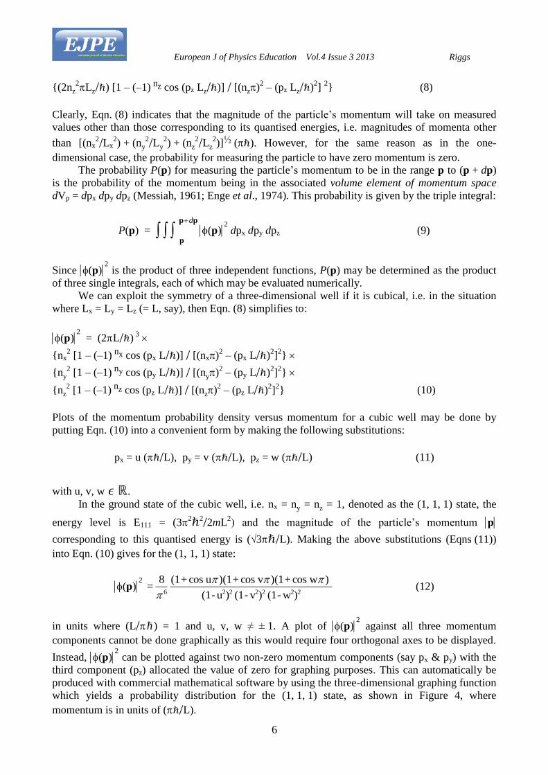
Clearly, Eqn. (8) indicates that the magnitude of the particle’s momentum will take on measured

values other than those corresponding to its quantised energies, i.e. magnitudes of momenta other

than [(nx2/Lx

2) + (ny

2/Ly2) + (nz

2/Lz2)]½ (ℏ). However, for the same reason as in the one-

dimensional case, the probability for measuring the particle to have zero momentum is zero.

The probability P(p) for measuring the particle’s momentum to be in the range p to (p + dp)

is the probability of the momentum being in the associated volume element of momentum space

dVp = dpx dpy dpz (Messiah, 1961; Enge et al., 1974). This probability is given by the triple integral:

P(p) = pp

p

d

(p)2 dpx dpy dpz (9)

Since (p)2 is the product of three independent functions, P(p) may be determined as the product

of three single integrals, each of which may be evaluated numerically.

We can exploit the symmetry of a three-dimensional well if it is cubical, i.e. in the situation

where Lx = Ly = Lz (= L, say), then Eqn. (8) simplifies to:

(p)2 = (2L/ℏ)

3

{nx2 [1 – (–1) nx cos (px L/ℏ)] / [(nx)

2 – (px L/ℏ)

2]2}

{ny2 [1 – (–1) ny cos (py L/ℏ)] / [(ny)

2 – (py L/ℏ)

2]2}

{nz2 [1 – (–1) nz cos (pz L/ℏ)] / [(nz)

2 – (pz L/ℏ)

2]

2} (10)

Plots of the momentum probability density versus momentum for a cubic well may be done by

putting Eqn. (10) into a convenient form by making the following substitutions:

px = u (ℏ/L), py = v (ℏ/L), pz = w (ℏ/L) (11)

with u, v, w ∊ ℝ.

In the ground state of the cubic well, i.e. nx = ny = nz = 1, denoted as the (1, 1, 1) state, the

energy level is E111 = (32ℏ2/2mL

2) and the magnitude of the particle’s momentum p

corresponding to this quantised energy is (√3ℏ/L). Making the above substitutions (Eqns (11))

into Eqn. (10) gives for the (1, 1, 1) state:

(p)2

2222226 )w-(1 )v-(1 )u-(1

) wcos+)(1 vcos+)(1u cos+(1

8 =

(12)

in units where (L/h ) = 1 and u, v, w ≠ ± 1. A plot of (p)2 against all three momentum

components cannot be done graphically as this would require four orthogonal axes to be displayed.

Instead, (p)2 can be plotted against two non-zero momentum components (say px & py) with the

third component (pz) allocated the value of zero for graphing purposes. This can automatically be

produced with commercial mathematical software by using the three-dimensional graphing function

which yields a probability distribution for the (1, 1, 1) state, as shown in Figure 4, where

momentum is in units of (ℏ/L).


7

Figure 4: (p)

2 vs. px, py (pz = 0) for the cubic ‘infinite’ well in the (1, 1, 1) state

Such figures are particularly useful for they provide a visual representation of the momentum

probability density in a regular, three-dimensional ‘infinite’ well and help appreciate the

distribution of probability over the chosen momentum ranges. Fig. 4 shows that the (1, 1, 1) state

has a central peak, analogous to the sole curve found in the ground state of the one-dimensional

case. This probability distribution indicates that the particle’s momentum is likely to be found with

its components each lying in the range of: – 2.0 to + 2.0. The maximum value of (p)2 is about

0.067, in units of (L/ℏ) = 1. The distribution also indicates that the measured magnitudes of

momentum are likely to be less than (√3ℏ/L). Indeed, since the probability of finding the value of

the particle’s momentum in given volume element of momentum space is largest when (p)2 is

greatest (Messiah 1961), it follows that the most probable values of the particle’s momentum in the

(1, 1, 1) state are close (but not equal) to zero.

Although momentum probabilities can be determined from such graphics, more accurate

probability values are obtainable by numerical integration. Probability values corresponding to

specific momentum ranges may be obtained by placing Eqn. (9) into a convenient form by making

the substitutions set out in Eqns (11). Integrations can then be performed numerically in order to

calculate probabilities for states of the cubic ‘infinite’ well. Upon making these substitutions,

Eqn. (9) becomes:

P(p) = 2

1

w

w

2

1

v

v

2

1

u

u

(u,v,w)2 du dv dw (13)

where the limits of integration are the intervals for each momentum component expressed in units

of (ℏ/L) = 1. Numerical integration of (p)2 allows the calculation of the probability of finding

the particle’s momentum in a particular state with its components lying in the ranges specified.

Commercial mathematical software can achieve this result by making three numerical integrations

and finding their product.

Probabilities for the (1, 1, 1) state may be obtained by integrating (p)2 as given by

Eqn. (12). Over suitably large intervals of the momentum components, the total probability in this


8

state is unity (as required by normalization). Table 1 displays a selection of a range of values of u,

v, w with the corresponding (numerically calculated) probability P(p) of finding the particle’s

momentum with its components lying in the specified ranges. 2 The range of p that corresponds to

these components is also given. Note that the probability value need not apply uniquely to the

corresponding p range (see also the discussion in Section 4).

Table 1: A selection of momentum probabilities for the cubic ‘infinite’ well in the (1, 1, 1) state

u v w P(p) p

0 — 4.0 0 — 4.0 0 — 4.0 0.124 0 — 4√3

– 1.0 — + 1.0 – 1.0 — + 1.0 – 1.0 — + 1.0 0.340 0 — √3

– 2.0 — + 2.0 – 2.0 — + 2.0 – 2.0 — + 2.0 0.913 0 — 2√3

– 5.0 — + 5.0 – 5.0 — + 5.0 – 5.0 — + 5.0 0.997 0 — 5√3

Probabilities for other desired ranges of u, v, and w are readily generated by this method.

Table 1 confirms the inference made from Fig. 4 that the momentum values likely to be measured

are those when all components lie in the range: – 2.0 to + 2.0. Note that when all three momentum

components have only positive values, the probability is significantly lower due to the

corresponding (three-dimensional) volume element of momentum space being much smaller than

for those ranges that include both positive and negative values.

The next energy level of the cubic well occurs with states for which one of the quantum

numbers is 2 and the others are 1. These states are degenerate with energy of (32ℏ

2/mL2), i.e. twice

the energy of the (1, 1, 1) state. Energy degenerate states in the cubic well are a direct result of its

symmetry and this has been suitably discussed in the literature (e.g. Saxon 1968; Beckhoff, 1976;

Greenhow 1990; Dahl, 2001; Blinder, 2004). The magnitude of the momentum corresponding to the

quantised energy is (√6ℏ/L). If we choose nx = 2 and ny = nz = 1, i.e. the (2, 1, 1) state, and make

the suggested substitutions (Eqns (11)), then Eqn. (10) becomes:

p)2

2222226 )w-(1 )v-(1 )u-(4

) wcos+)(1 vcos+)(1u cos-(1

32 =

(14)

where u ≠ ± 2 and v, w ≠ ± 1. Figure 5 is a plot of (p)2 against two non-zero components (px & py

≠ 0, pz = 0) in the (2, 1, 1) state.

2 All numerical integrations were performed with Mathematica (Version 8).


9

Figure 5: (p)

2 vs. px, py (pz = 0) for the cubic ‘infinite’ well in the (2, 1, 1) state

It can be seen from Fig. 5 that the (2, 1, 1) state has two peaks (analogous to the n = 2 state in the

one-dimensional case), which are only about two-thirds of the height of the (1, 1, 1) peak. The

maximum value of (p)2 is about 0.045, in units of (L/ℏ) = 1. The distribution indicates that the

particle’s momentum is most likely to be found with px close (or equal) to ± (1.67)(ℏ/L), and the

other components close to zero. It follows that the most probable magnitude of momentum in this

state is less than (√6ℏ/L).

Probabilities may be calculated for the (2, 1, 1) state by numerical integration using Eqn. (14),

i.e. by following the same procedure as performed above for the (1, 1, 1) state. Table 2 shows a

selection of momentum ranges with the corresponding probability P(p) of finding the particle’s

momentum with its components lying in the specified ranges. The range of p that corresponds to

these components is also given but, as previously noted, the probability value need not apply

uniquely to the corresponding p range.


u v w P(p) p

0 — 3.0 0 — 3.0 0 — 3.0 0.118 0 — 3√3

0 — 3.0 – 3.0 — + 3.0 – 3.0 — + 3.0 0.471 0 — 3√3

– 1.0 — + 1.0 – 1.0 — + 1.0 – 1.0 — + 1.0 0.067 0 — √3

– 2.0 — + 2.0 – 2.0 — + 2.0 – 2.0 — + 2.0 0.596 0 — 2√3

– 3.5 — + 3.5 – 3.5 — + 3.5 – 3.5 — + 3.5 0.977 0 — (3.5) √3

– 5.0 — + 5.0 – 5.0 — + 5.0 – 5.0 — + 5.0 0.992 0 — 5√3

Table 2 confirms the visual inference from Fig. 5 that the probability distribution falls

symmetrically into two equal parts. This can be seen from the second row where the probability is

nearly one-half for intervals that take in about half of the distribution. The low probability found

when the three momentum components each have the range of: – 1.0 to + 1.0 (third row), can be

seen in Fig. 5 to be due to this distribution having a trough.


10

The next energy level of the cubic well without degeneracy is the state in which nx = ny = nz =

2, i.e. the (2, 2, 2) state. This state has an energy of E222 = (62ℏ

2/mL2), i.e. twice the energy of the

(2, 1, 1) state. The magnitude of the momentum corresponding to the quantised energy is

(2√3ℏ/L). If we make the suggested substitutions (Eqns (11)) for the (2, 2, 2) state, then Eqn. (10)

becomes:

(p)2

2222226 )w-(4 )v-(4 )u-(4

) wcos-)(1 vcos-)(1u cos-(1

512 =

(15)

where u , v, w ≠ ± 2. Figure 6 is a graph of the (2, 2, 2) state where (p)2 is plotted against the

components px & py with pz given a constant non-zero value. This is necessary as assigning pz = 0

would yield (p)2 = 0 (as may be seen from Eqn. (15)). In Fig. 6, the (constant) value for w is

chosen to give the same scaling for (p)2 as used for previous figures to allow comparison between

the figures.

Figure 6: (p)

2 vs. px, py (pz = constant) for the cubic ‘infinite’ well in the (2, 2, 2) state

It can be seen from Fig. 6 that the (2, 2, 2) state has four peaks positioned symmetrically about the

origin (analogous to the n = 4 state in the one-dimensional case), which are about one-quarter of the

height of the (2, 1, 1) peaks. This distribution also shows that the maximum value of (p)2 is about

0.012, in units of (L/ℏ) = 1, and that the particle’s momentum is most likely to be found with all

momentum components near or equal to ± (1.9)(ℏ/L). It follows that the most probable magnitude

of momentum in this state is slightly less than (2√3ℏ/L).

Probabilities may be calculated for the (2, 2, 2) state by numerical integration using Eqn. (15).

Table 3 shows a selection of momentum ranges with the corresponding probability P(p) of finding

the particle’s momentum with its components lying in the specified ranges. The range of p that

corresponds to these components is also given (previous comments regarding p apply).


11


u v w P(p) p

0 — 3.5 0 — 3.5 0 — 3.5 0.120 0 — (3.5) √3

0 — 3.5 – 3.5 — + 3.5 – 3.5 — + 3.5 0.479 0 — (3.5) √3

– 1.0 — + 1.0 – 1.0 — + 1.0 – 1.0 — + 1.0 0.0026 0 — √3

– 2.0 — + 2.0 – 2.0 — + 2.0 – 2.0 — + 2.0 0.253 0 — 2√3

– 3.5 — + 3.5 – 3.5 — + 3.5 – 3.5 — + 3.5 0.958 0 — (3.5) √3

– 5.0 — + 5.0 – 5.0 — + 5.0 – 5.0 — + 5.0 0.983 0 — 5√3

Table 3 (first and second rows) confirms the visual inference from Fig. 6 that the probability

distribution falls symmetrically into four equal parts. It can also be seen from Fig. 6 that the low

probability found when all three momentum components each have the range: – 1.0 to + 1.0 (third

row) is due to two central troughs in the distribution.

Probabilities of Measuring Specific Magnitudes of Particle Momenta

There are a few comments to be made on the probabilities of measured particle momenta in three-

dimensional, rectangular ‘infinite’ wells that will assist in understanding their significance.

First, as should be obvious from entries in Tables 2 – 4, the ranges of p are indifferent to

whether the ranges of the momentum components cover both positive and negative values or not. In

Table 4, for example, the first row has each component with the range: 0 — + 3.5, and the fifth row

has each component with the range: – 3.5 — + 3.5. Despite having very different probabilities

(0.120 and 0.958 respectively), both entries in the table have the same range of p. Second, the arrangement of detectors in a given experimental set-up will be a primary

determining factor as to what probabilities should be expected. If, for instance, measurements are

made which cover all of a cubic ‘infinite’ well (e.g. the sides, top and bottom of an atom trap) then

the probabilities given in Tables 2 – 4 will be applicable. If the arrangement of detectors is such that

only the momentum in a particular direction is measured then this obviously needs to be taken into

account and the expected probabilities will be lower.

Third, it is regularly the case that measurements of a particle’s momentum are only

measurements of the magnitude of the total momentum p (or of other quantities, e.g. particle

speed, from which p may be deduced) rather than measurements of the momentum components.

Eqn. (8) shows that because (p)2 depends explicitly on the components of p (rather than on p

itself), different values of (p)2 can arise for the same p depending on what individual values px,

py, and pz take. When very different values of (p)2 occur for the same value of p, one of the

(p)2 values will be at least an order of magnitude larger than the others and therefore the smaller

values of (p)2 will have a negligible contribution to the probabilities.

Concluding Remarks

A selection of momentum probability densities for three-dimensional regular ‘infinite’ potential

wells were provided and plotted. Representative numerical values of momentum probabilities also

were calculated and discussed. The techniques employed in this paper can be easily extended to

states of the cubic ‘infinite’ well with higher quantum numbers than the states examined and

(somewhat laboriously) to rectangular ‘infinite’ wells with unequal side lengths. The results and


12

techniques presented should assist students in gaining a better understanding momentum probability

densities and the utilisation of momentum space descriptions of quantum systems.

These results and techniques might be implemented, for example, by designing class exercises

that require students to:

Derive the momentum probability density function (Eqn. (4)) given the normalised,

configuration space eigenfunctions (Eqn. (1)) for a one-dimensional ‘infinite’ well;

Using the graphing tool in commercial mathematical software, plot graphs of momentum

probability density versus momentum for various values of the quantum number n;

Find the numerical probabilities for the particle’s momentum to be found in specified

momentum ranges by measuring areas under various curves in the plotted graphs;

Compare some of these probability values with those found by manually integrating simple

one-dimensional cases;

Generalise the one-dimensional momentum probability density function to its three-

dimensional form (Eqn. (8));

Describe how the three-dimensional probability density relates to momentum space;

By making suitable substitutions of variables, find a form of the three-dimensional

probability density function that is practical for graphing purposes;

Using the three-dimensional graphing tool in commercial mathematical software, plot

graphs of momentum probability densities against momentum components for various three-

dimensional ‘infinite’ wells;

Suggest a technique by which numerical integration might be performed for three-

dimensional cases that have been graphed;

Perform the suggested numerical integrations using commercial mathematical software and

relate the results to the plotted graphs.

References

Auletta, G., Fortunato, M. and Parisi, G. (2009). Quantum Mechanics. Cambridge: Cambridge

University Press.

Basdevant, J. L., Dalibard, J. (2002). Quantum Mechanics. Berlin: Springer.

Beckhoff, F. J. (1976). Elements of Quantum Theory (2nd

edition). Reading, MA.: Addison-Wesley.

Bes, D.R. (2007). Quantum Mechanics: A Modern and Concise Introductory Course. Berlin:

Springer.

Blinder, S.M. (2004). Introduction to Quantum Mechanics in Chemistry, Materials Science, and

Biology. Amsterdam: Elsevier.

Braginsky, V.B. and Khalili, F.Y. (ed. K.S. Thorne) (1992). Quantum Measurement. Cambridge:

Cambridge University Press.

Cohen-Tannoudji, C., Diu, B. and Laloe, F. (1977). Quantum Mechanics. New York: Wiley.

Crommie, M.F., Lutz, C.P., Eigler, D.M. (1993). Confinement of Electrons to Quantum Corrals on

a Metal Surface. Science, 262, 218-220.

Cummings, F.E. (1977). The Particle in a Box is not simple. American Journal of Physics, 63 (2),

158-160.

Dahl, J.P. (2001). Introduction to the Quantum World of Atoms and Molecules. Singapore: World

Scientific.

Dowling, J.P. and Gea-Banacloche, J. (1995). Schrödinger modal structure of cubical, pyramidal,

and conical, evanescent light-wave gravitational atom traps. Physical Review A, 52, 3997-

4003.

Eisberg, R.M. (1961). Fundamentals of Modern Physics. New York: Wiley.

Eisberg, R. and Resnick, R. (1985). Quantum Physics of Atoms, Molecules, Solids, Nuclei, and

Particles (2nd

edition). New York: Wiley.


13

Enge, H.A., Wehr, M.R. and Richards, J.A. (1974). Introduction to Atomic Physics. Reading, MA:

Addison-Wesley.

Gasiorowicz, S. (1974). Quantum Physics. New York: Wiley.

Greenhow, R.C. (1990). Introductory Quantum Mechanics: A Computer Illustrated Text Bristol &

New York: Adam Hilger.

Griffiths, D.J. (2005). Introduction to Quantum Mechanics. Upper Saddle N.J.: Pearson.

Henkel, C., Courtois, J. Y., Kaiser, R., Westbrook, C. and Aspect, A. (1994). Phase shifts of atomic

de Broglie waves at an evanescent wave mirror. Laser Physics, 4 (5), 1042-1049.

Kippeny, T., Swafford, L.A. and Rosenthal, S.J. (2002). Semiconductor Nanocrystals: A Powerful

Visual Aid for Introducing the Particle in a Box. Journal of Chemical Education, 79 (9),

1094-1100.

Liang, Y. Q., Zhang, H. and Dardenne, Y.X. (1995). Momentum Distributions for a Particle in a

Box. Journal of Chemical Education, 72 (2), 148-151.

Markley, F.L. (1972). Probability Distributions of Momenta in an Infinite Square-Well Potential.

American Journal of Physics. 40 (Oct.), 1545-1546.

Messiah, A. (1961). Quantum Mechanics (Vol. 1) Amsterdam: North Holland.

Meyrath, T.P., Schreck, F., Hanssen, J.L., Chu, C.-S. and Raisin, M.G. (2005). Bose-Einstein

Condensate in a Box. Physical Review A, 71, 041604 (R).

Robinett, R.W. (1995). Quantum and Classical Probability Distributions for Position and

Momentum. American Journal of Physics, 63 (9), 823-832.

Robinett, R.W. (1997). Quantum Mechanics: Classical Results, Modern Systems and Visualized

Examples. Cambridge: Cambridge University Press.

Robinett, R.W. (2002). Visualizing Classical and Quantum Probability Densities for Momentum

Using Variations on Familiar One-dimensional Potentials. European Journal of Physics 23,

165-174.

Sadaghiani, H., Bao, L. (2006). Student Difficulties in Understanding Probability in Quantum

Mechanics. In: P. Heron, L. McCullough and J. Marx (Eds), 2005 Physics Education

Research Conference: AIP Conference Proceedings 818 (pp.61-64). American Institute of

Physics. Downloadable at: extras.springer.com/2006/978-0-7354-0311-

6/cdr_pdfs_indexed_stage4_copyr_61_1.pdf

Saxon, D.S. (1968). Elementary Quantum Mechanics. San Francisco: Holden-Day.

Schiff, L.I. (1968). Quantum Mechanics. Tokyo: McGraw-Hill Kogakusha.

Vos, M. and Weigold, E. (2002). Particle-in-a-box momentum densities compared with electron

momentum spectroscopy measurements. Journal of Electron Spectroscopy and Related

Phenomena, 123, 333-344.

Zettili, N. (2009). Quantum Mechanics: Concepts and Applications. Chichester, UK: Wiley.

Documents

1 Momentum Probabilities for a Single Quantum Particle in Three