1

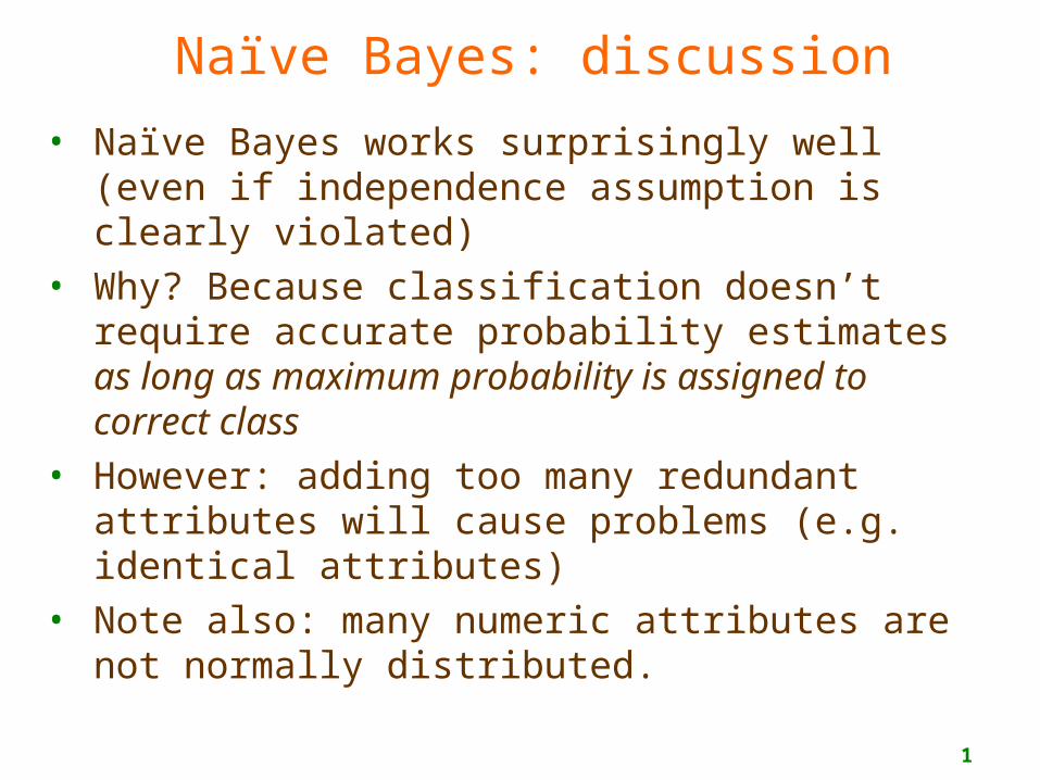
Naïve Bayes: discussion

• Naïve Bayes works surprisingly well (even if independence assumption is clearly violated)

• Why? Because classification doesn’t require accurate probability estimates as long as maximum probability is assigned to correct class

• However: adding too many redundant attributes will cause problems (e.g. identical attributes)

• Note also: many numeric attributes are not normally distributed.

2

Decision trees

• another statistical, supervised learning technique

• builds a model from training data – the model is a decision tree.

• internal nodes query the attributes

• leaf nodes announce the class of the instance

3

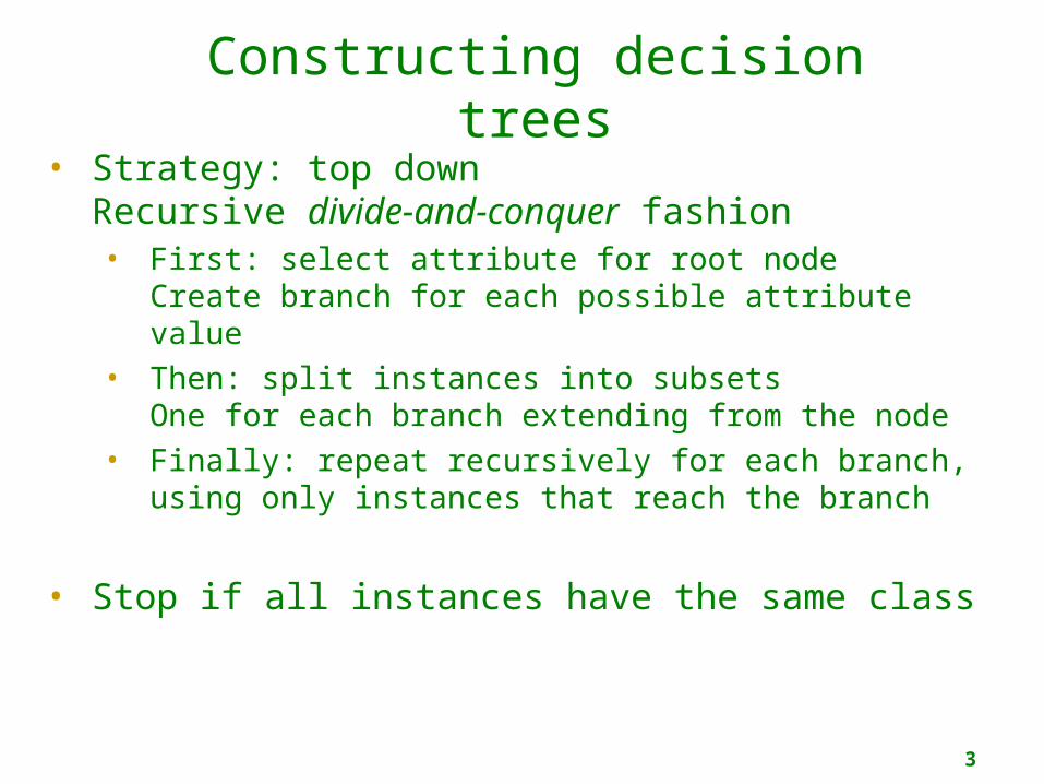
Constructing decision trees

• Strategy: top downRecursive divide-and-conquer fashion• First: select attribute for root node

Create branch for each possible attribute value• Then: split instances into subsets

One for each branch extending from the node• Finally: repeat recursively for each branch,

using only instances that reach the branch

• Stop if all instances have the same class

4

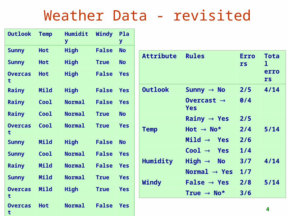
Weather Data - revisited

Attribute Rules Errors

Total errors

Outlook Sunny No 2/5 4/14

Overcast Yes

0/4

Rainy Yes 2/5

Temp Hot No* 2/4 5/14

Mild Yes 2/6

Cool Yes 1/4

Humidity High No 3/7 4/14

Normal Yes 1/7

Windy False Yes 2/8 5/14

True No* 3/6

Outlook Temp Humidity

Windy

Play

Sunny Hot High False No

Sunny Hot High True No

Overcast

Hot High False Yes

Rainy Mild High False Yes

Rainy Cool Normal False Yes

Rainy Cool Normal True No

Overcast

Cool Normal True Yes

Sunny Mild High False No

Sunny Cool Normal False Yes

Rainy Mild Normal False Yes

Sunny Mild Normal True Yes

Overcast

Mild High True Yes

Overcast

Hot Normal False Yes

Rainy Mild High True No

5

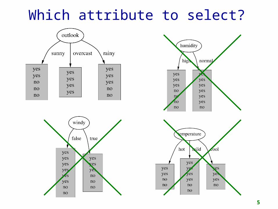
Which attribute to select?

6

Criterion for attribute selection

o Which is the best attribute?o Want to get the smallest treeo Heuristic: choose the attribute that produces

the “purest” nodes

o Popular impurity criterion: information gaino Information gain increases with the average

purity of the subsets

o Strategy: choose attribute that gives greatest information gain

7

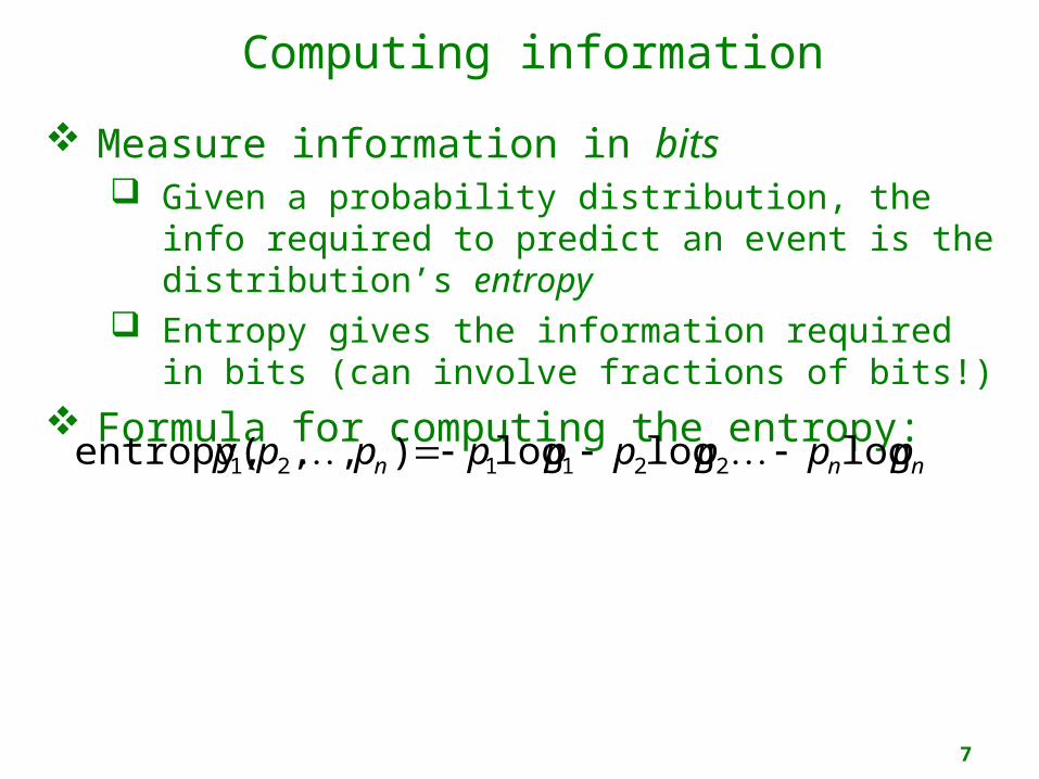
Computing information

Measure information in bits Given a probability distribution, the info

required to predict an event is the distribution’s entropy

Entropy gives the information required in bits (can involve fractions of bits!)

Formula for computing the entropy:

entropy(p1, p2,, pn ) p1logp1 p2logp2 pnlogpn

Entropy measure: some examples

As the data become purer and purer, the entropy value becomes smaller and smaller. This is useful to us!

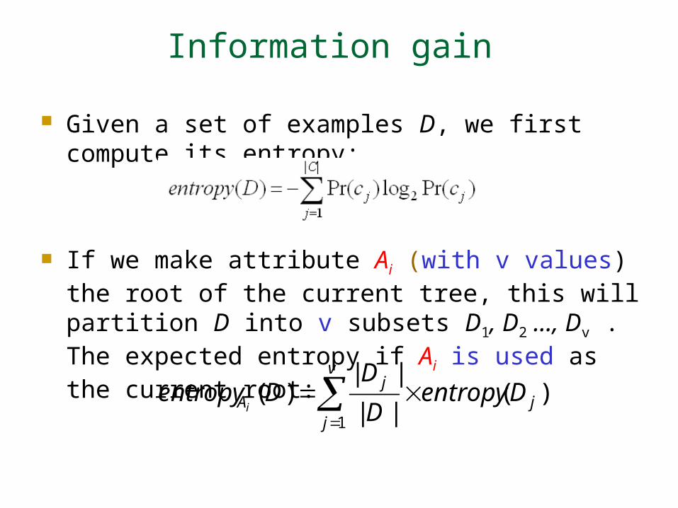
Information gain

Given a set of examples D, we first compute its entropy:

If we make attribute Ai (with v values) the root of the current tree, this will partition D into v subsets D1, D2 …, Dv . The expected entropy if Ai is used as the current root:

v

jj

jA Dentropy

D

DDentropy

i

1

)(||

||)(

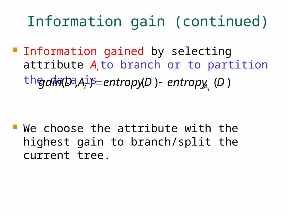
Information gain (continued)

Information gained by selecting attribute Ai

to branch or to partition the data is

We choose the attribute with the highest gain to branch/split the current tree.

)()(),( DentropyDentropyADgainiAi

11

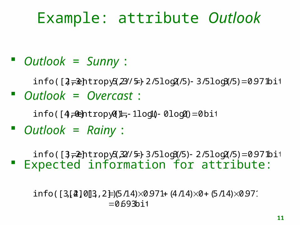
Example: attribute Outlook

Outlook = Sunny :

Outlook = Overcast :

Outlook = Rainy :

Expected information for attribute:

bits 971.0)5/3log(5/3)5/2log(5/25,3/5)entropy(2/)info([2,3]

bits 0)0log(0)1log(10)entropy(1,)info([4,0]

bits 971.0)5/2log(5/2)5/3log(5/35,2/5)entropy(3/)info([3,2]

971.0)14/5(0)14/4(971.0)14/5([3,2])[4,0],,info([3,2] bits 693.0

12

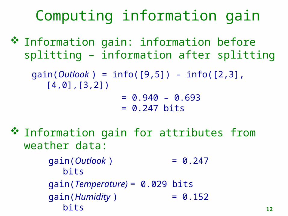
Computing information gain

Information gain: information before splitting – information after splitting

Information gain for attributes from weather data:

gain(Outlook ) = 0.247 bitsgain(Temperature) = 0.029 bitsgain(Humidity ) = 0.152 bitsgain(Windy ) = 0.048 bits

gain(Outlook ) = info([9,5]) – info([2,3],[4,0],[3,2]) = 0.940 – 0.693 = 0.247 bits

13

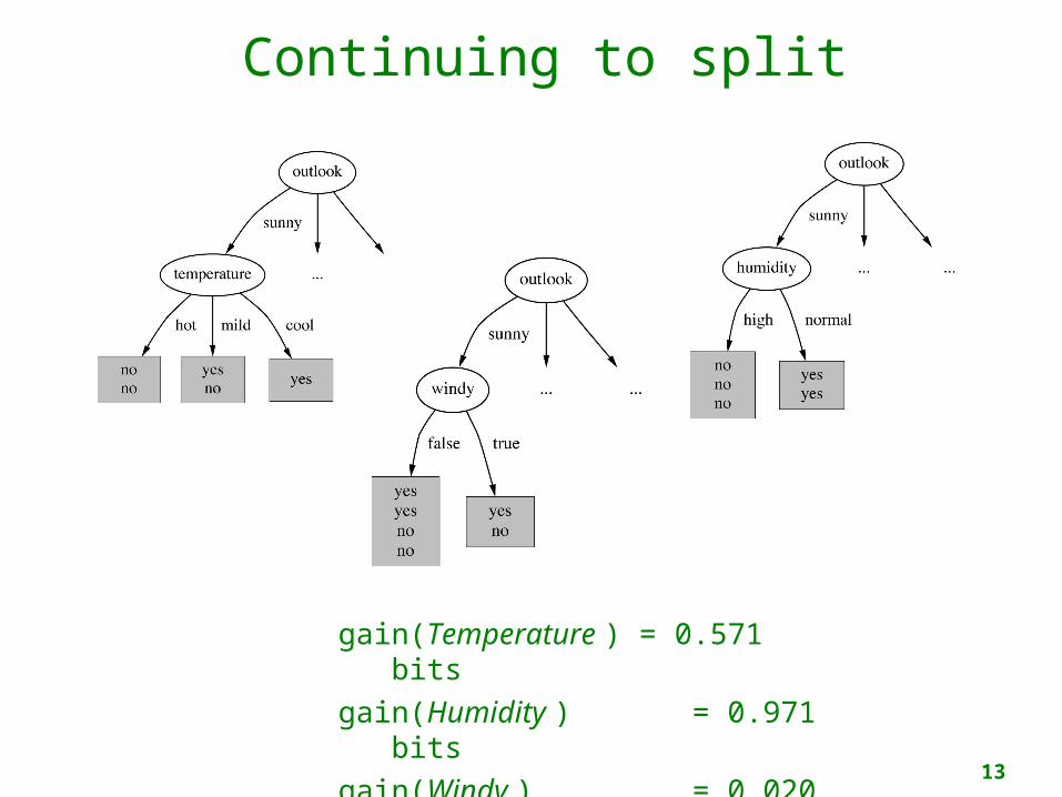
Continuing to split

gain(Temperature ) = 0.571 bitsgain(Humidity ) = 0.971

bitsgain(Windy ) = 0.020

bits

14

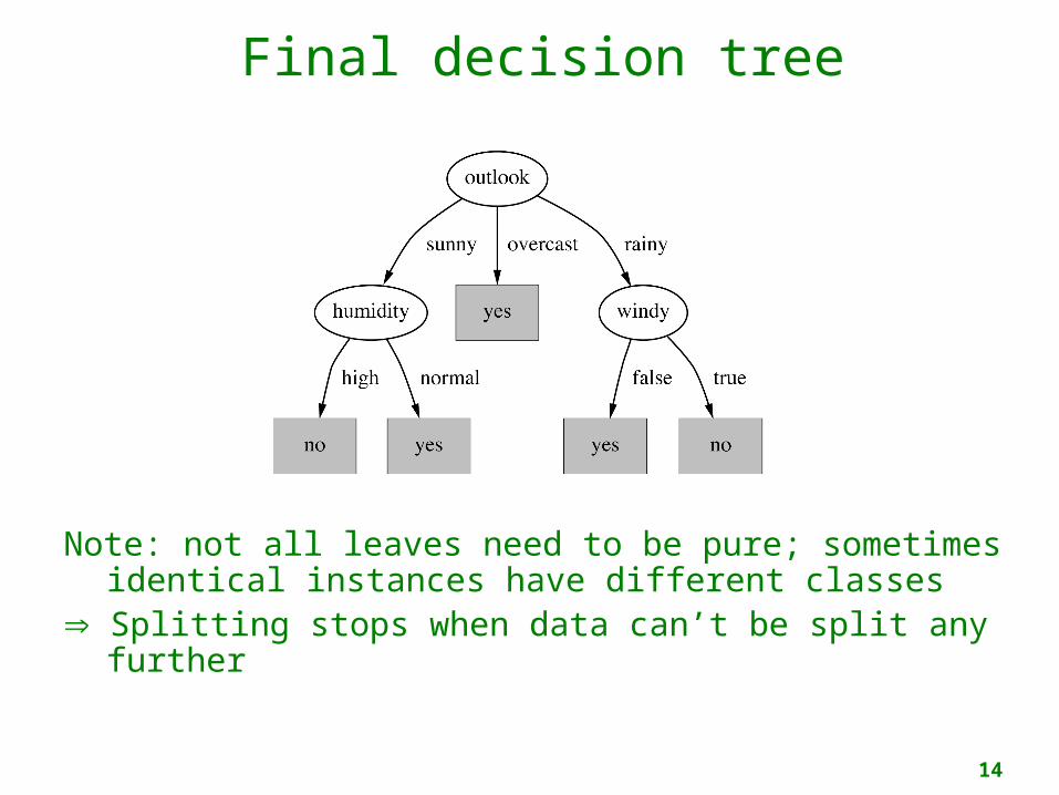
Final decision tree

Note: not all leaves need to be pure; sometimes identical instances have different classes

Splitting stops when data can’t be split any further

15

Another example

Age Yes No entropy(Di)young 2 3 0.971middle 3 2 0.971old 4 1 0.722

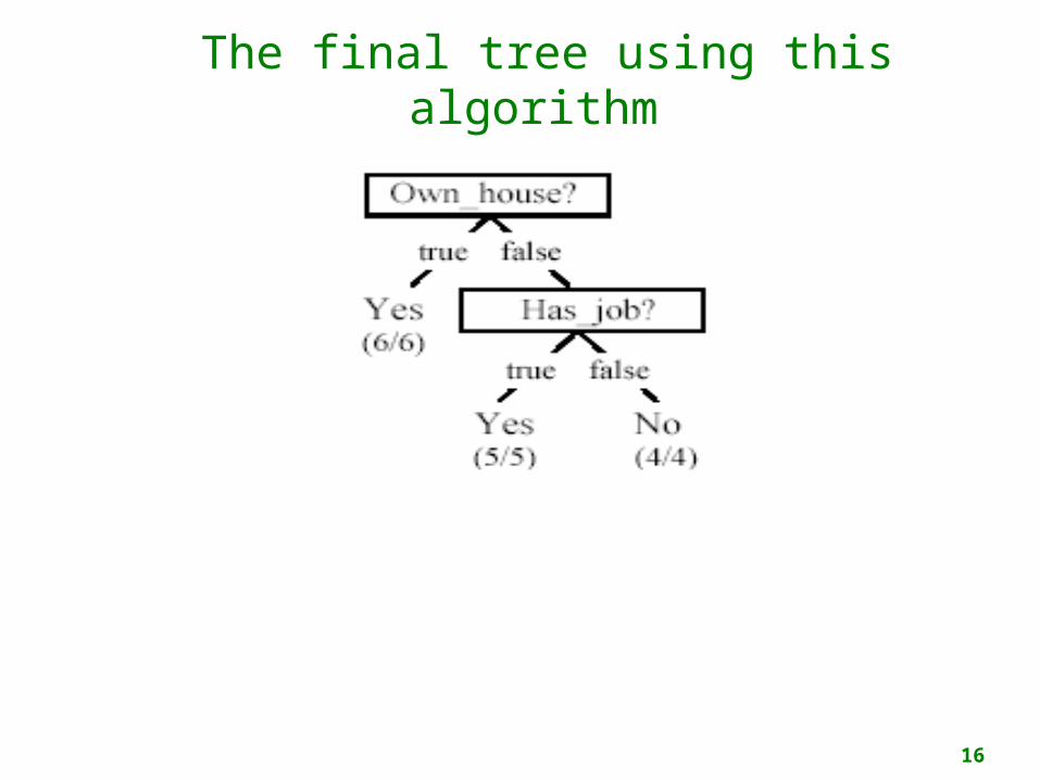
Own_house is the best choice for the root.

971.015

9log

15

9

15

6log

15

6)( 22 Dentropy

551.0

918.015

90

15

6

)(15

9)(

15

6)( 21_

DentropyDentropyDentropy houseOwn

888.0

722.015

5971.0

15

5971.0

15

5

)(15

5)(

15

5)(

15

5)( 321

DentropyDentropyDentropyDentropy Age

16

The final tree using this algorithm

17

Another example - information theory

There are 7 coins of which one of them is heavier or lighter than the other.

The rest are all of identical weight. All the coins look alike and we want to identify the odd

coin by weighing on a scale by comparing the weights of one group of coins against another group.

Consider the following options for the first weighing: (a) weighing coins 1, 2, 3 vs. 4, 5, 6 (b) weighing coins 1, 2 vs. 3, 4.

What are the reductions in the entropies associated with the two options?

18 18

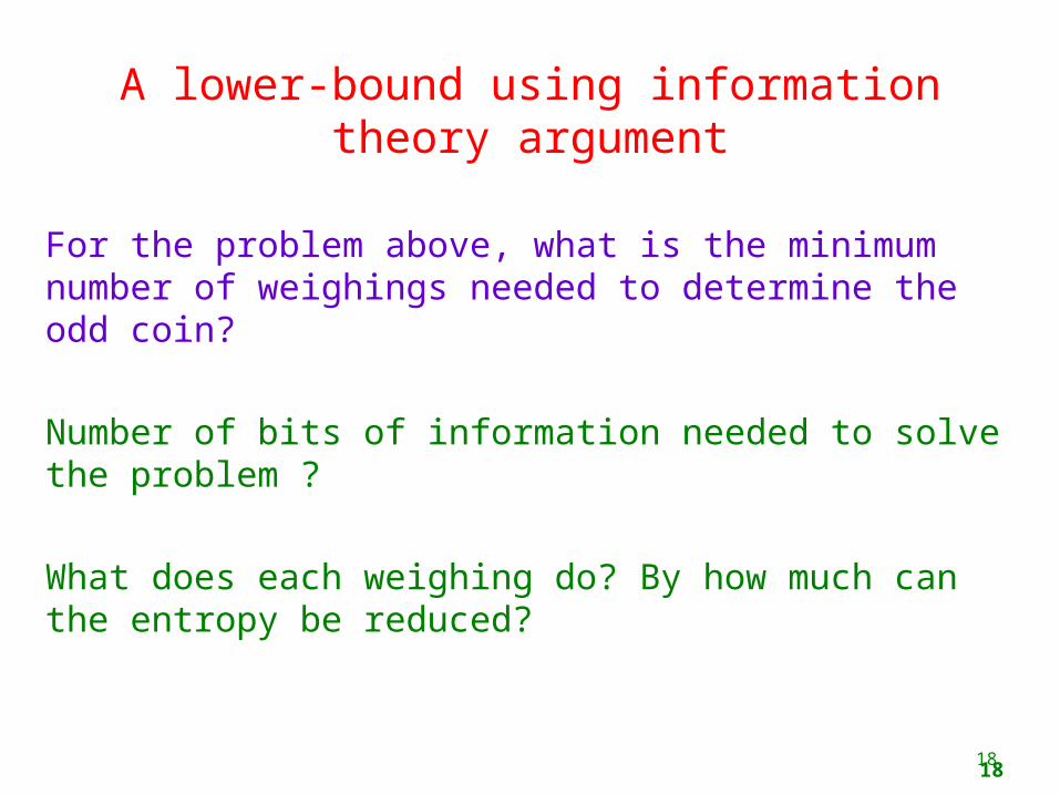
A lower-bound using information theory argument

For the problem above, what is the minimum number of weighings needed to determine the odd coin?

Number of bits of information needed to solve the problem ?

What does each weighing do? By how much can the entropy be reduced?

19

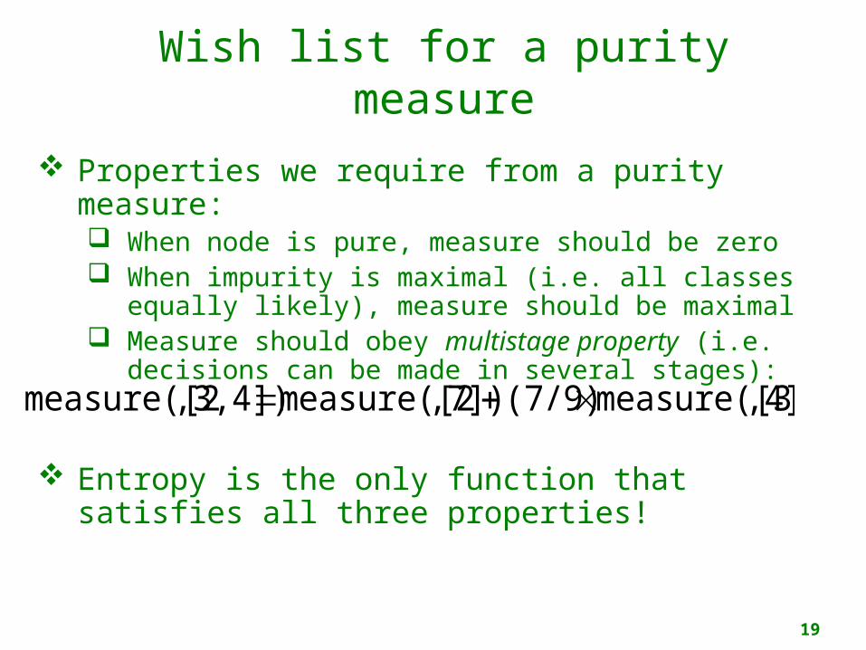
Wish list for a purity measure

Properties we require from a purity measure: When node is pure, measure should be zero When impurity is maximal (i.e. all classes

equally likely), measure should be maximal Measure should obey multistage property (i.e.

decisions can be made in several stages):

Entropy is the only function that satisfies all three properties!

,4])measure([3(7/9),7])measure([2,3,4])measure([2

20

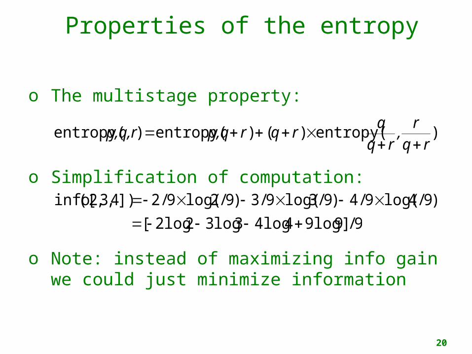
Properties of the entropy

o The multistage property:

o Simplification of computation:

o Note: instead of maximizing info gain we could just minimize information

)entropy()()entropy()entropy(rqr

,rqq

rqrp,qp,q,r

)9/4log(9/4)9/3log(9/3)9/2log(9/2])4,3,2([info 9/]9log94log43log32log2[

21

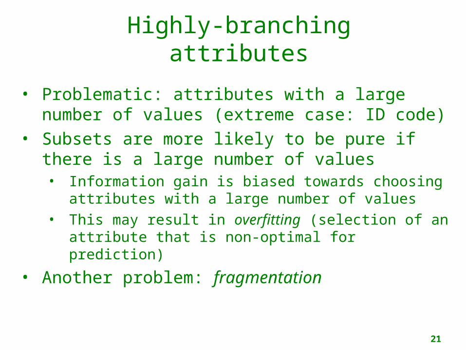
Highly-branching attributes

• Problematic: attributes with a large number of values (extreme case: ID code)

• Subsets are more likely to be pure if there is a large number of values• Information gain is biased towards choosing

attributes with a large number of values• This may result in overfitting (selection of an

attribute that is non-optimal for prediction)

• Another problem: fragmentation

22

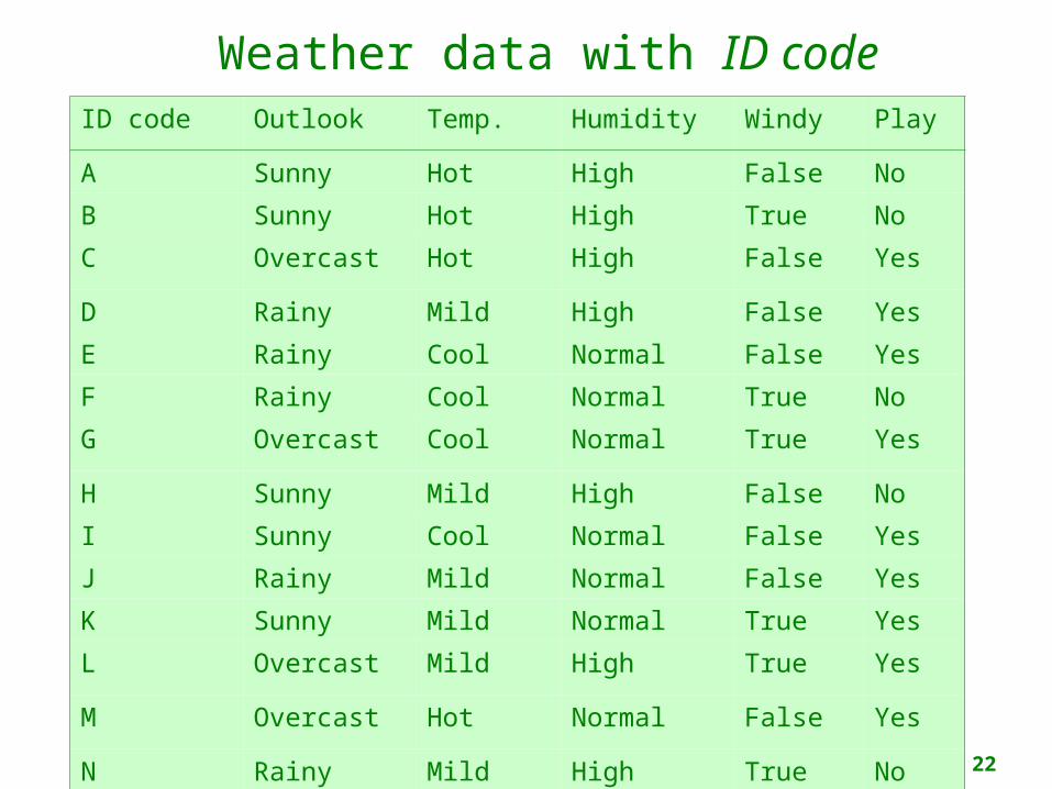
Weather data with ID codeID code Outlook Temp. Humidity Windy Play

A Sunny Hot High False No

B Sunny Hot High True No

C Overcast Hot High False Yes

D Rainy Mild High False Yes

E Rainy Cool Normal False Yes

F Rainy Cool Normal True No

G Overcast Cool Normal True Yes

H Sunny Mild High False No

I Sunny Cool Normal False Yes

J Rainy Mild Normal False Yes

K Sunny Mild Normal True Yes

L Overcast Mild High True Yes

M Overcast Hot Normal False Yes

N Rainy Mild High True No

23

Tree stump for ID code attribute

Entropy of split:

Information gain is maximal for ID code (namely 0.940 bits)

info("ID code") info([0,1]) info([0,1]) info([0,1]) 0 bits

24

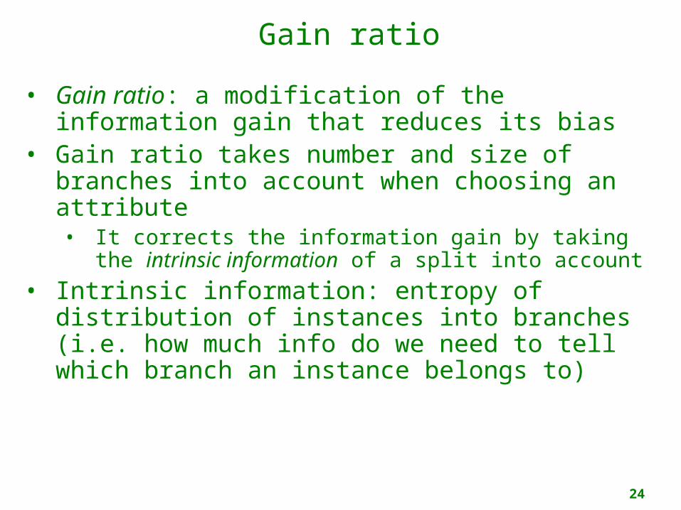
Gain ratio

• Gain ratio: a modification of the information gain that reduces its bias

• Gain ratio takes number and size of branches into account when choosing an attribute• It corrects the information gain by taking the

intrinsic information of a split into account

• Intrinsic information: entropy of distribution of instances into branches (i.e. how much info do we need to tell which branch an instance belongs to)

25

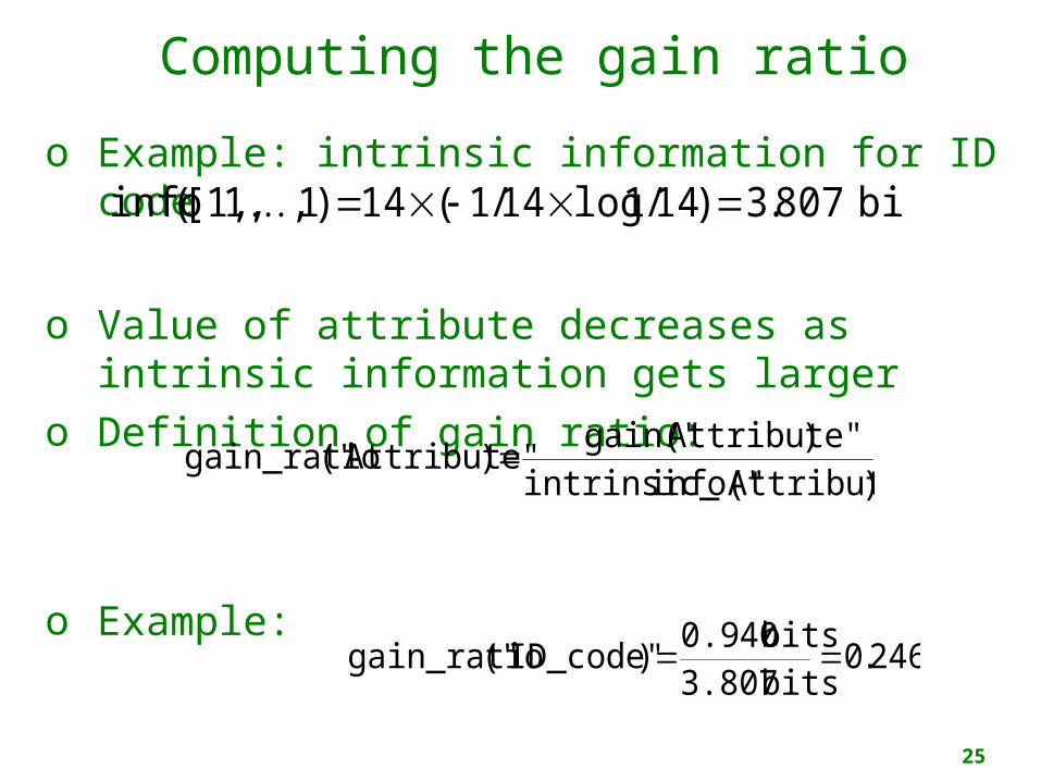
Computing the gain ratio

o Example: intrinsic information for ID code

o Value of attribute decreases as intrinsic information gets larger

o Definition of gain ratio:

o Example:

info([1,1,,1) 14 ( 1/14 log1/14) 3.807 bits

)Attribute"info("intrinsic_)Attribute"gain("

)Attribute"("gain_ratio

246.0bits 3.807bits 0.940

)ID_code"("gain_ratio

26

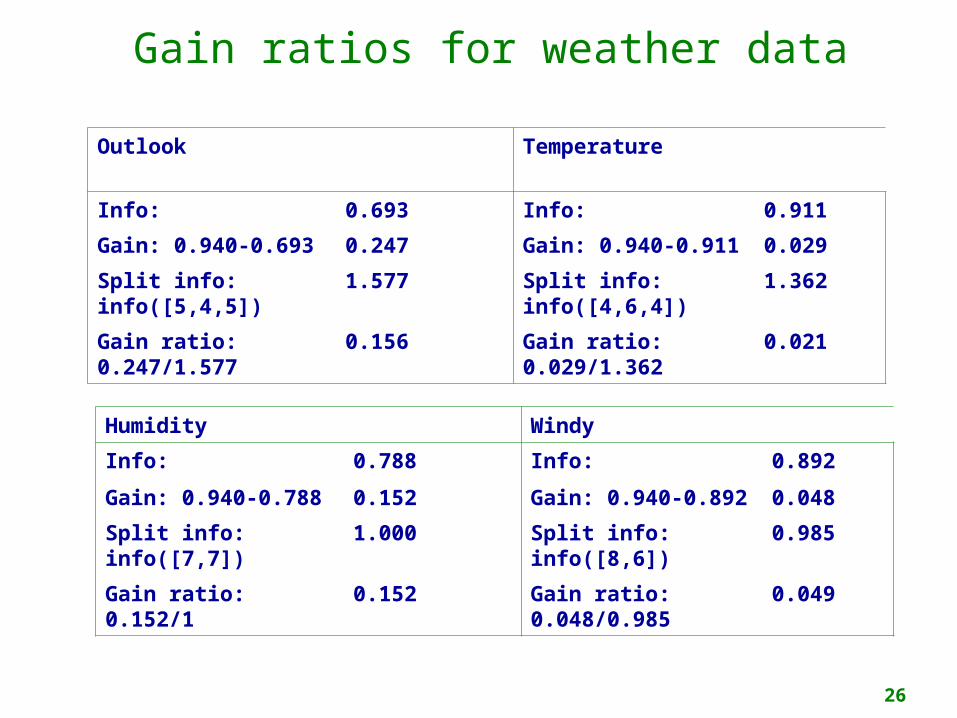
Gain ratios for weather data

Outlook Temperature

Info: 0.693 Info: 0.911

Gain: 0.940-0.693 0.247 Gain: 0.940-0.911 0.029

Split info: info([5,4,5])

1.577 Split info: info([4,6,4])

1.362

Gain ratio: 0.247/1.577

0.156 Gain ratio: 0.029/1.362

0.021

Humidity Windy

Info: 0.788 Info: 0.892

Gain: 0.940-0.788 0.152 Gain: 0.940-0.892 0.048

Split info: info([7,7])

1.000 Split info: info([8,6])

0.985

Gain ratio: 0.152/1 0.152 Gain ratio: 0.048/0.985

0.049

27

More on the gain ratio

o “Outlook” still comes out topo However: “ID code” has greater gain ratio

o Standard fix: ad hoc test to prevent splitting on that type of attribute

o Problem with gain ratio: it may overcompensateo May choose an attribute just because its

intrinsic information is very lowo Standard fix: only consider attributes with

greater than average information gain

28

Discussion

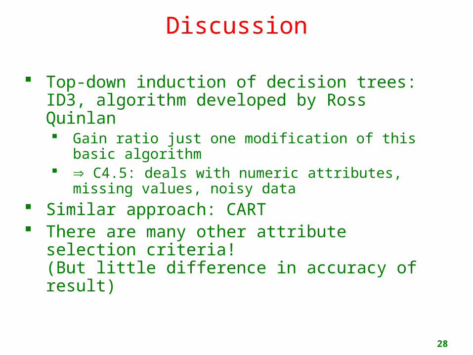
Top-down induction of decision trees: ID3, algorithm developed by Ross Quinlan Gain ratio just one modification of this basic

algorithm C4.5: deals with numeric attributes,

missing values, noisy data Similar approach: CART There are many other attribute selection

criteria!(But little difference in accuracy of result)

29

Covering algorithms

• Convert decision tree into a rule set• Straightforward, but rule set overly complex• More effective conversions are not trivial

• Instead, can generate rule set directly• for each class in turn find rule set that covers

all instances in it(excluding instances not in the class)

• Called a covering approach:• at each stage a rule is identified that “covers”

some of the instances

30

Example: generating a rule

y

x

a

b b

b

b

b

bb

b

b b bb

bb

aa

aa

ay

a

b b

b

b

b

bb

b

b b bb

bb

a a

aa

a

x1·2

y

a

b b

b

b

b

bb

b

b b bb

bb

a a

aa

a

x1·2

2·6

If x > 1.2then class = a

If x > 1.2 and y > 2.6then class = a

If truethen class = a

Possible rule set for class “b”:

Could add more rules, get “perfect” rule set

If x 1.2 then class = bIf x > 1.2 and y 2.6 then class = b

31

Rules vs. treeso Corresponding decision tree:

(produces exactly the same predictions)

o But: rule sets can be more perspicuous when decision trees suffer from replicated subtrees

o Also: in multiclass situations, covering algorithm concentrates on one class at a time whereas decision tree learner takes all classes into account

32

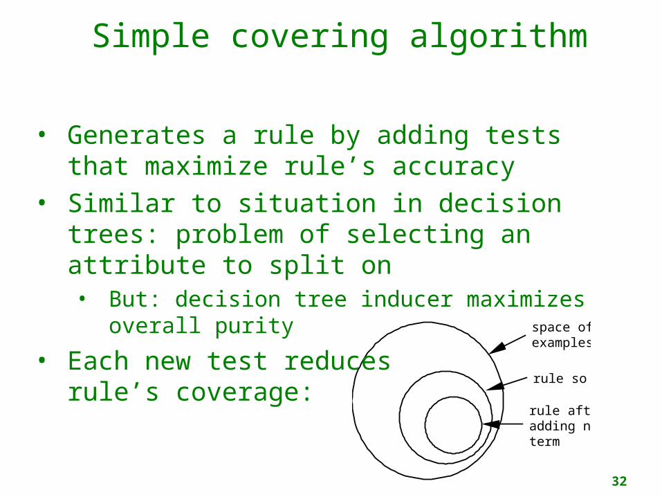
space of examples

rule so far

rule after adding new term

Simple covering algorithm

• Generates a rule by adding tests that maximize rule’s accuracy

• Similar to situation in decision trees: problem of selecting an attribute to split on• But: decision tree inducer maximizes

overall purity

• Each new test reducesrule’s coverage:

33

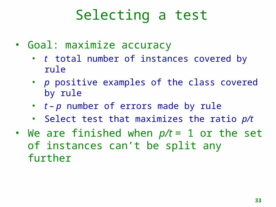
Selecting a test

• Goal: maximize accuracy• t total number of instances covered by rule• p positive examples of the class covered by

rule• t – p number of errors made by rule• Select test that maximizes the ratio p/t

• We are finished when p/t = 1 or the set of instances can’t be split any further

34

Example: contact lens data

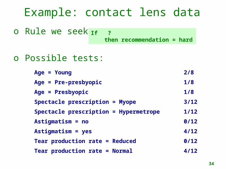
o Rule we seek:

o Possible tests:

Age = Young 2/8

Age = Pre-presbyopic 1/8

Age = Presbyopic 1/8

Spectacle prescription = Myope 3/12

Spectacle prescription = Hypermetrope 1/12

Astigmatism = no 0/12

Astigmatism = yes 4/12

Tear production rate = Reduced 0/12

Tear production rate = Normal 4/12

If ? then recommendation = hard

35

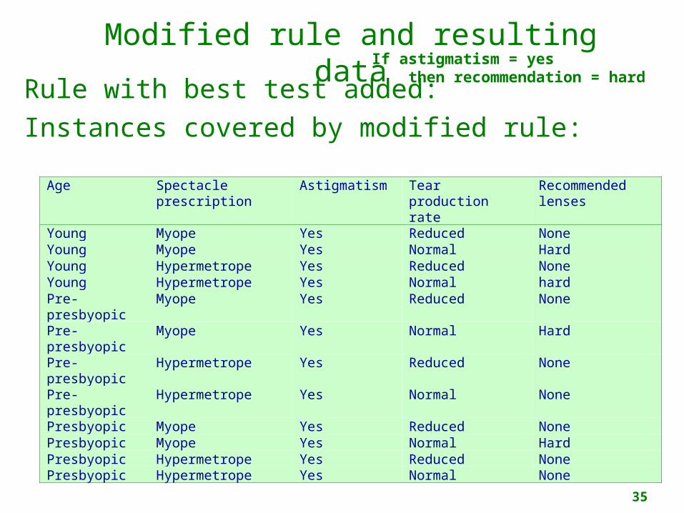
Modified rule and resulting data

Rule with best test added:Instances covered by modified rule:

Age Spectacle prescription

Astigmatism Tear production rate

Recommended lenses

Young Myope Yes Reduced NoneYoung Myope Yes Normal HardYoung Hypermetrope Yes Reduced NoneYoung Hypermetrope Yes Normal hardPre-presbyopic

Myope Yes Reduced None

Pre-presbyopic

Myope Yes Normal Hard

Pre-presbyopic

Hypermetrope Yes Reduced None

Pre-presbyopic

Hypermetrope Yes Normal None

Presbyopic Myope Yes Reduced NonePresbyopic Myope Yes Normal HardPresbyopic Hypermetrope Yes Reduced NonePresbyopic Hypermetrope Yes Normal None

If astigmatism = yes then recommendation = hard

36

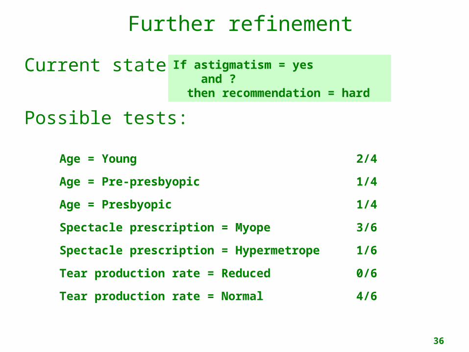
Further refinement

Current state:

Possible tests:

Age = Young 2/4

Age = Pre-presbyopic 1/4

Age = Presbyopic 1/4

Spectacle prescription = Myope 3/6

Spectacle prescription = Hypermetrope 1/6

Tear production rate = Reduced 0/6

Tear production rate = Normal 4/6

If astigmatism = yes and ? then recommendation = hard

37

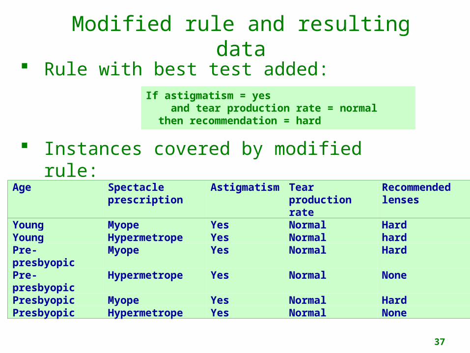
Modified rule and resulting data

Rule with best test added:

Instances covered by modified rule:

Age Spectacle prescription

Astigmatism

Tear production rate

Recommended lenses

Young Myope Yes Normal HardYoung Hypermetrope Yes Normal hardPre-presbyopic

Myope Yes Normal Hard

Pre-presbyopic

Hypermetrope Yes Normal None

Presbyopic Myope Yes Normal HardPresbyopic Hypermetrope Yes Normal None

If astigmatism = yes and tear production rate = normal then recommendation = hard

38

Further refinement

o Current state:

o Possible tests:

o Tie between the first and the fourth testo We choose the one with greater coverage

Age = Young 2/2

Age = Pre-presbyopic 1/2

Age = Presbyopic 1/2

Spectacle prescription = Myope 3/3

Spectacle prescription = Hypermetrope 1/3

If astigmatism = yes and tear production rate = normal and ?then recommendation = hard

39

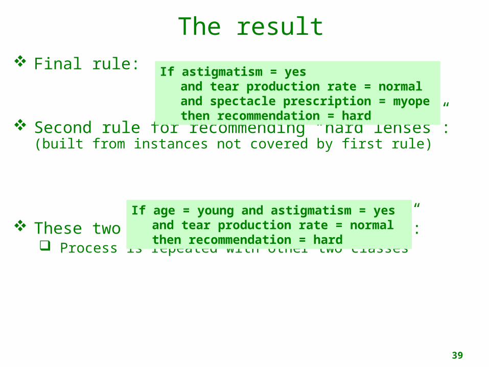
The result Final rule:

Second rule for recommending “hard lenses”:(built from instances not covered by first rule)

These two rules cover all “hard lenses”: Process is repeated with other two classes

If astigmatism = yesand tear production rate = normaland spectacle prescription = myopethen recommendation = hard

If age = young and astigmatism = yesand tear production rate = normalthen recommendation = hard