1

Nonlinear Camera Response Functions and ImageDeblurring: Theoretical Analysis and Practice

Yu-Wing Tai1 Xiaogang Chen2,5 Sunyeong Kim1 Seon Joo Kim3 Feng Li4

Jie Yang2 Jingyi Yu5 Yasuyuki Matsushita6 Michael S. Brown71KAIST, 2Shanghai Jiao Tong University, 3Yonsei University, 4MERL,

5University of Delaware, 6MSRA, 7National University of Singapore

Abstract— This paper investigates the role that nonlinearcamera response functions (CRFs) have on image deblurring. Wepresent a comprehensive study to analyze the effects of CRFs onmotion deblurring. In particular, we show how nonlinear CRFscan cause a spatially invariant blur to behave as a spatiallyvarying blur. We prove that such nonlinearity can cause largeerrors around edges when directly applying deconvolution toa motion blurred image without CRF correction. These errorsare inevitable even with a known point spread function (PSF)and with state-of-the-art regularization based deconvolution al-gorithms. In addition, we show how CRFs can adversely affectPSF estimation algorithms in the case of blind deconvolution. Tohelp counter these effects, we introduce two methods to estimatethe CRF directly from one or more blurred images when the PSFis known or unknown. Our experimental results on synthetic andreal images validate our analysis and demonstrate the robustnessand accuracy of our approaches.

Index Terms— Nonlinear Camera Response Functions (CRFs),Motion Deblurring, CRF Estimation

I. I NTRODUCTION

Image deblurring is a long standing computer vision problemfor which the goal is to recover a sharp image from a blurredimage. Mathematically, the problem is formulated as:

B = I ⊗K + n, (1)

whereB is the captured blurred image,I is the latent image,Kis the point spread function (PSF),⊗ is the convolution operator,andn represents image noise.

One common assumption in most previous algorithms that isoften overlooked is that the imageB in Equation (1) respondsin a linear fashion with respect to irradiance,i.e., the final imageintensity is proportional to the amount of light received by thesensor. This assumption is valid when we capture an image in aRAW format. However, when capturing an image using a commonconsumer level camera or camera on a mobile device, there is anonlinear camera response function(CRF) that maps the sceneirradiance to intensity. CRFs vary among different camera man-ufacturers and models due to design factors such as compressingthe scene’s dynamic range or to simulate conventional irradianceresponses of film [15], [33]. Taking this nonlinear response intoaccount, the imaging process of Equation (1) can be consideredas:

B = f(I ⊗K + n), (2)

wheref(·) is the CRF. To remove the effect of the nonlinear CRFfrom image deblurring, the imageB has to be first linearizedby the inverse CRF,i.e., f−1. After deconvolution, the CRF is

applied again to restore the original intensity which leads to thefollowing process:

I = f(f−1(B)⊗K−1), (3)

where K−1 is inverse filter which denotes the deconvolutionprocess.

Contributions This paper offers two contributions with regardsto CRFs and their role in image deblurring. First, we providea systematic analysis of the effect that a CRF has on theblurring process and show how a nonlinear CRF can make aspatially invariant blur behave as a spatially varying blur aroundedges. We prove that such nonlinearity can cause abrupt ringingartifacts around edges which are non-uniform. In addition, theseartifacts are difficult to eliminated by regularization. Our analysisalso shows that PSF estimation for various blind deconvolutionalgorithms are adversely affected by the nonlinear CRF.

Along with the theoretical analysis, we further introduce twoalgorithms to estimate the CRF from one or more images: thefirst method is based on a least-square formation when the PSF isknown; the second method is formulated as a rank minimizationproblem when the PSF is unknown. Both of these approachesexploit the relationship between the blur profile about edges ina linearized image and the PSF. While our estimation methodscannot compete with well-defined radiometric calibration methodsbased on calibration patterns or multiple exposures, they areuseful to produce a sufficiently accurate CRF for improvingdeblurring results.

Shorter versions of this work appeared in [22], [7]. This paperunifies these two concurrent independent works with more in-depth discussion and analysis of the role of CRF in deblur-ring, and additional experiments. In addition, a new sectionthat analyzes the effectiveness of gamma curve correction intraditional deblurring methods, and the limitations of the proposedalgorithms are presented in Section VII-A.

The remainder of our paper is organized as follow: In Sec-tion II, we review related works in motion deblurring and CRFestimation. Our theoretical analysis about the blur inconsistencyintroduced by a nonlinear CRF is presented in Section III, fol-lowed by the analysis on the deconvolution artifacts and PSF es-timation errors in Section IV. Our two algorithms which estimatethe nonlinear CRF from motion blurred image(s) with knownand unknown PSF are presented in Section V. In Section VI,we present our experimental results. Section VII-A providesadditional discussion about the effectiveness of gamma curvecorrection. Finally, we conclude our work in Section VIII.

2

I I. RELATED WORK

Image deblurring is a classic problem with well-studied ap-proaches including Richardson-Lucy [35], [40] and Wiener de-convolution [48]. Recently, several different directions were in-troduced to enhance the performance of deblurring. These includemethods that use image statistics [14], [29], [18], [6], sparsityor sharp edge prediction [30], [20], [8], [2], [50], [26], [45],multiple images or hybrid imaging systems [1], [39], [9], [51],[5], [42], [43], and new blur models that account for cameramotion [44], [46], [47], [19], [17]. The vast majority of thesemethods, however, do not consider the nonlinearity in the imagingprocess due to CRFs.

The goal of radiometric calibration is to compute a CRFfrom a given set of images or a single image. The most accu-rate radiometric calibration algorithms use multiple images withdifferent exposures [12], [4], [37], [13], [15], [21], [24], [34],[28]. Our work is more related to single-image based radiometriccalibration techniques [32], [33], [38], [36], [49]. In [32], the CRFis computed by observing the color distributions of local edgeregions: the CRF is computed as the mapping that transformsnonlinear distributions of edge colors into linear distributions.This idea is further extended to deal with a single gray-scaleimage using histograms of edge regions in [33]. In [49], a CRFis estimated by temporally mixing of a step edge within a singlecamera exposure by the linear motion blur of a calibration pattern.Unlike [49], however, our method deals with uncontrolled blurredimages.

To the best of our knowledge, there are only a handful ofprevious works that consider CRFs in the context of imagedeblurring. Examples include the work by Ferguset al. [14],where images are first linearized by an inverse gamma-correctionwith γ = 2.2. Real world CRFs, however, are often drasticallydifferent from gamma curves [15], [31]. Another example by Luetal. [34] involves reconstructing a high dynamic range image froma set of differently exposed and possibly motion blurred images.Work by Cho et al. [10] discussed nonlinear CRFs as a causefor artifacts in deblurring, but provided little insight into whysuch artifacts arise. Their work suggested to avoid this by usinga pre-calibrated CRF or the camera’s RAW output. While a pre-calibrated CRF is undoubtedly the optimal solution, the CRF maynot always be available. Moreover, work by Chakrabartiet al. [3]suggests that a CRF may be scene dependent when the camera isin “ auto mode”. Furthermore, work by Kimet al. [23] showedthat the CRF for a given camera may vary for different camerapicture styles (e.g., landscape, portrait, etc).

Our work aims to provide more insight into the effect thatCRFs have on the image deblurring process. In addition, we seekto provide a method to estimate a CRF from a blurred input imagein the face of a missing or unreliable pre-calibrated CRF.

III. B LUR INCONSISTENCY DUE TO NONLINEARCRF

We first study the role of the CRF in the image blurring process.We denote byf as the nonlinear CRF,f−1 as the inverse off ,I as the blur-free intensity image,I as the irradiance image ofI, i.e., I = f(I), B as the observed motion blurred image withB = f(I ⊗ K + n). To focus our analysis, we follow previouswork by assuming that the PSF is spatially invariant and the imagenoise is negligible (i.e., n ≈ 0).

We analyze the blur inconsistency introduced by a nonlinearCRF by measuring:

Γ = B − B (4)

whereB = I⊗K which denotes the conventional intensity basedblurring process. Note thatI is used instead ofI in B. Our goalin here is to understand where the intensity based convolutionmodel would introduce errors when CRF correction is excluded.

Claim 1. In uniform intensity regions,Γ = 0 .Proof: Since pixels within the blur kernel region have uniformintensity, we havef−1(I) ⊗ K = f−1(I) = f−1(I ⊗ K).Therefore,

B = f(f−1(I)⊗K) = f(f−1(I ⊗K)) = B, (5)

thusΓ = 0.Claim 1 applies to any CRF (both linear or nonlinear). This

implies that a nonlinear CRF will not affect deblurring qualityfor uniform intensity regions.

Claim 2. If the blur kernelK is small and the CRFf issmooth,Γ ≈ 0 in low frequency regions.Proof: Let I = I + ∆I be a local patch covered by the blurkernel K. The termI is the average intensity within the patchand∆I is the deviation fromI. In low frequency regions,∆I issmall.

Next, we apply the first-order Taylor series expansion tof−1(I)⊗K as:

f−1(I +∆I)⊗K ≈ f

−1(I)⊗K + (f ′−1(I) ·∆I)⊗K, (6)

wheref ′−1 is the first order derivative off−1. SinceI is uniform,we havef−1(I) ⊗ K = f−1(I) and f ′−1(I) is constant in thelocal neighborhood. Thus, Equation (6) can be approximated as:

f−1(I) + f

′−1(I) ·∆I ⊗K. (7)

Similarly, by using the first-order Taylor series expansion, wehave

f−1(I ⊗K) = f

−1(I ⊗K +∆I ⊗K)

≈ f−1(I ⊗K) + f

′−1(I ⊗K) · (∆I ⊗K)(8)

= f−1(I) + f

′−1(I) ·∆I ⊗K. (9)

Therefore,

B = f(f−1(I)⊗K) ≈ f(f−1(I ⊗K)) = B, (10)

i.e., Γ ≈ 0.Claim 2 holds only for small kernels. When the kernel size

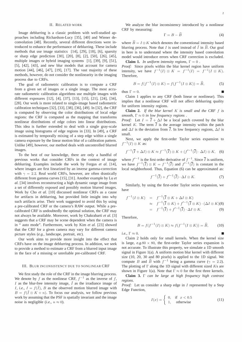
is large,e.g.80 × 80, the first-order Taylor series expansion isnot accurate. To illustrate this property, we simulate a 1D smoothsignal in Figure 1(a). A uniform motion blur kernel with differentsize (10, 20, 30 and 80 pixels) is applied to the 1D signal. WecomputeB and B with f−1 being a gamma curve (γ = 2.2).The plotting ofΓ along the 1D signal with different sizedKs areshown in Figure 1(a). Note thatΓ ≈ 0 for the first three kernels.

Claim 3. Γ can be large at high frequency high contrastregions.Proof: Let us consider a sharp edge inI represented by a StepEdge Function,

I(x) =

{0, if x < 0.5

1, otherwise(11)

3

(a) (b) (c)

0

0.3

smooth signalΓ(length=10)Γ(length=20)Γ(length=30)Γ(length=80)

0

1.0

sharp signalΓ(length=10)Γ(length=20)Γ(length=30)Γ(length=80)

0 300 0 500

Fig. 1. Illustration of blur inconsistencyΓ. A gamma curve withγ = 2.2 is used to simulatef−1 across all sub-figures. (a):Γ is computed along a1D smooth signal with four different uniform motion blur kernels of size 10, 20, 30 and 80 pixels. (b) The first two rows show the latent pattern and thecorresponding irradiance-based motion blurred pattern respectively. The bottom row shows the measuredΓ which varies across different edge strength. (c)Plotting ofΓ in (b) with different kernel sizes.

0 0.15 0.3 0.45 0.6 0.75 0.90

0.15

0.3

0.45

0.6

0.75

0.9

irradiance

intensity

Fig. 2. The left panel shows 188 CRF curves of real cameras fromDoRF[15]. Nearly all curves appear concave.

Sincef−1 has boundaryf−1(0) = 0 and f−1(1) = 1 [15], wehavef−1(I) = I. Therefore,

B = f(f−1(I)⊗K) = f(I ⊗K) = f(B), (12)

Hence,Γ = f(B)− B.In this example,Γ(x) measures howf(x) deviates from the

linear functiony(x) = x. In other words,Γ(x) → 0, iff f(x) → x.However, practical CRFsf are highly nonlinear [15], [23].

To validate Claim 3, we simulate a 1D signal of sharp edgeswith different gradient magnitudes and measure the blur inconsis-tencyΓ as shown in Figure 1(b). The first row is the original clearsignal. The second row is the blur signalB where the blur kernelsize is 20 pixels. The third row shows theΓ which is non-zeroaround edge regions and theΓ increase as the gradient magnitudesget larger. To further analyze the effect of kernel size on sharpsignals, we plotΓ with four different sized kernels in Figure 1(c).Notice that the area of non-zeroΓ increase with kernel size sincethe blurry edge gets larger. Also, the magnitude ofΓ depends onedge magnitude but it does not depends on kernel size.

Theorem 1. Let Imin and Imax be the local minimum andmaximum pixel intensities in a local neighborhood covered bykernelK in imageI. If f−1 is convex, then the Blur Inconsistencyis bounded by0 ≤ Γ ≤ Imax − Imin.Proof: Considerf−1(I)⊗K as a convex combination of pixels

from f−1(I) sinceK contains only zero or positive values. Iff−1 is convex, we can use the Jensen’s inequality to obtain

f−1(I)⊗K ≥ f

−1(I ⊗K). (13)

Further, since the CRFf is a monotonically increasing [12], [37],we have:

B = f(f−1(I)⊗K) ≥ f(f−1(I ⊗K)) = B, (14)

i.e., Γ ≥ 0.Next, we derive the upper bound ofΓ. SinceI⊗K ≤ Imax and

f−1 is monotonically increasing (asf−1 is inverse off andf ismonotonically increasing),f−1(I)⊗K ≤ f−1(Imax). Therefore,we have,

B = f(f−1(I)⊗K) ≤ f(f−1(Imax)) = Imax. (15)

Likewise, we can also deriveB = I⊗K ≥ Imin. Combining thiswith Equation (14) and Equation (15), we have:Imin ≤ B ≤

B ≤ Imax. Therefore,

0 ≤ Γ ≤ Imax − B ≤ Imax − Imin. (16)

Theorem 1 explains the phenomenon in Figure 1: when thegradient magnitude of an edge is large, the upper-bound ofΓ

will be large. On the other hand, in low contrast regions, theupper boundImax − Imin is small and so isΓ. Thus,B can bewell approximated byB.

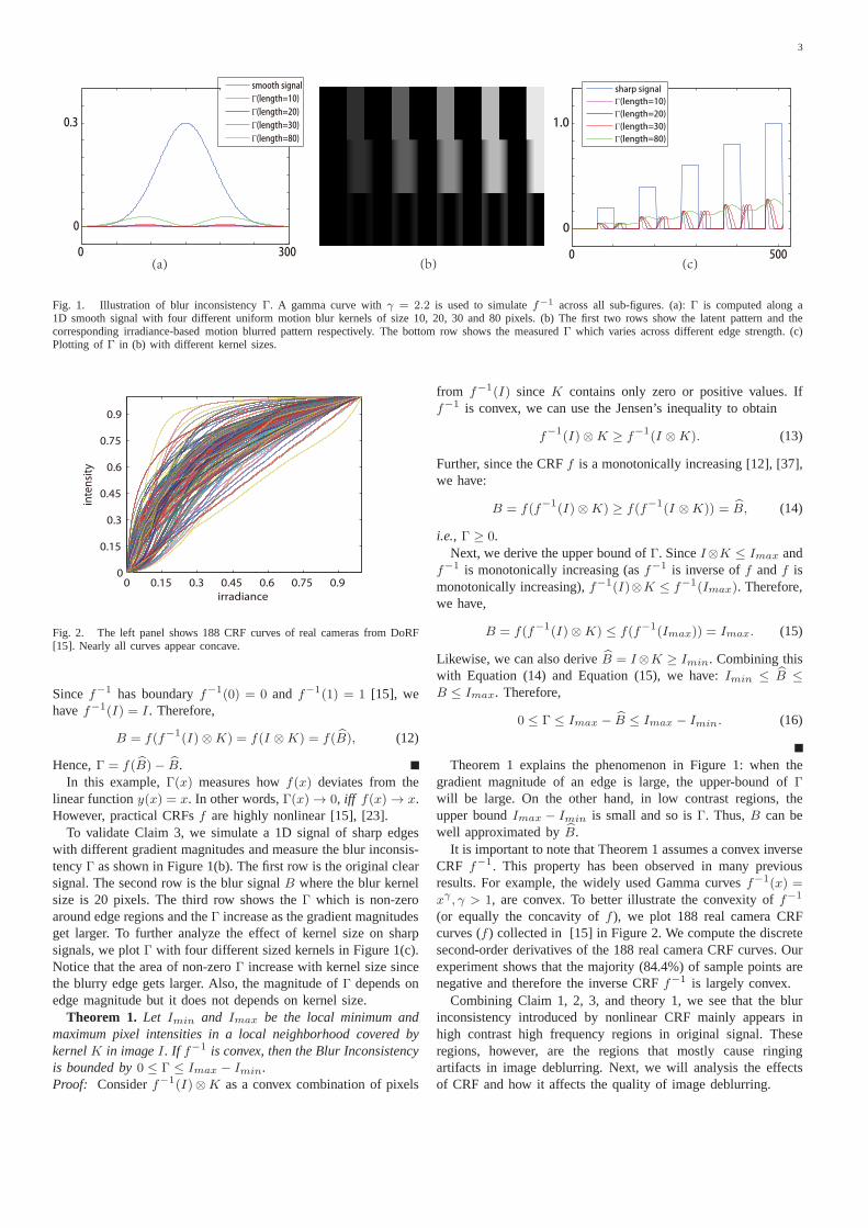
It is important to note that Theorem 1 assumes a convex inverseCRF f−1. This property has been observed in many previousresults. For example, the widely used Gamma curvesf−1(x) =

xγ , γ > 1, are convex. To better illustrate the convexity off−1

(or equally the concavity off), we plot 188 real camera CRFcurves (f) collected in [15] in Figure 2. We compute the discretesecond-order derivatives of the 188 real camera CRF curves. Ourexperiment shows that the majority (84.4%) of sample points arenegative and therefore the inverse CRFf−1 is largely convex.

Combining Claim 1, 2, 3, and theory 1, we see that the blurinconsistency introduced by nonlinear CRF mainly appears inhigh contrast high frequency regions in original signal. Theseregions, however, are the regions that mostly cause ringingartifacts in image deblurring. Next, we will analysis the effectsof CRF and how it affects the quality of image deblurring.

4

0 50 100 150 200 250 3000

1

PSF

0

1

0 50 100 150 200 250 300

0 50 100 150 200 250 300

0

1

0 50 100 150 200 250 3000

1

PSF

−1

0

1

0 50 100 150 200 250 300

0 50 100 150 200 250 300

0

1

0 50 100 150 200 250 3000

1

PSF

0

1

0 50 100 150 200 250 300

0 50 100 150 200 250 300

0

1

0 50 100 150 200 250 3000

1

PSF

−1

0

1

0 50 100 150 200 250 300

0 50 100 150 200 250 300

0

1

Linear CRF (kernel A) Nonlinear CRF (kernel A) Linear CRF (kernel B) Nonlinear CRF (kernel B)

Wiener Filter Result Wiener Filter Result

With Regularization

(a) (b) (c) (d)

(e) (f) (g) (h)

(i) (j) (k) (l)

With Regularization

PSF PSF PSF PSF

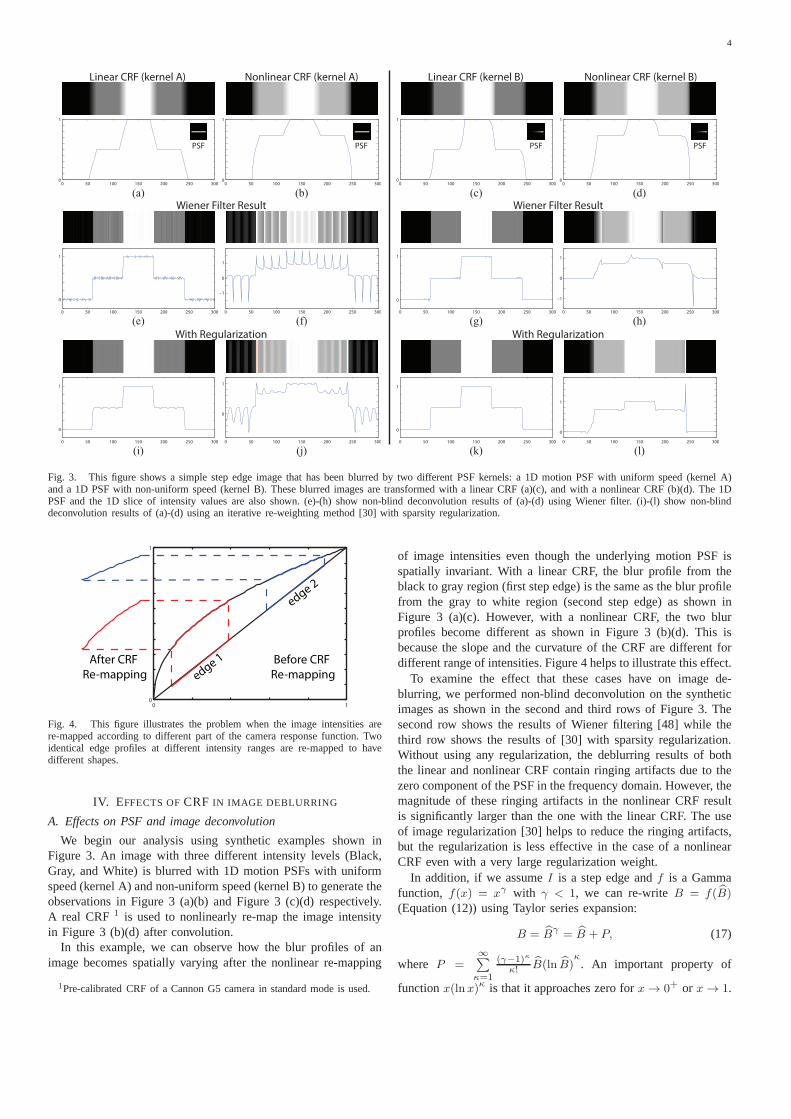
Fig. 3. This figure shows a simple step edge image that has been blurred by two different PSF kernels: a 1D motion PSF with uniform speed (kernel A)and a 1D PSF with non-uniform speed (kernel B). These blurred images are transformed with a linear CRF (a)(c), and with a nonlinear CRF (b)(d). The 1DPSF and the 1D slice of intensity values are also shown. (e)-(h) show non-blind deconvolution results of (a)-(d) using Wiener filter. (i)-(l) show non-blinddeconvolution results of (a)-(d) using an iterative re-weighting method [30] with sparsity regularization.

0 10

1

After CRF

Re-mapping

Before CRF

Re-mappingedge 1

edge 2

Fig. 4. This figure illustrates the problem when the image intensities arere-mapped according to different part of the camera response function. Twoidentical edge profiles at different intensity ranges are re-mapped to havedifferent shapes.

IV. EFFECTS OFCRF IN IMAGE DEBLURRING

A. Effects on PSF and image deconvolution

We begin our analysis using synthetic examples shown inFigure 3. An image with three different intensity levels (Black,Gray, and White) is blurred with 1D motion PSFs with uniformspeed (kernel A) and non-uniform speed (kernel B) to generate theobservations in Figure 3 (a)(b) and Figure 3 (c)(d) respectively.A real CRF1 is used to nonlinearly re-map the image intensityin Figure 3 (b)(d) after convolution.

In this example, we can observe how the blur profiles of animage becomes spatially varying after the nonlinear re-mapping

1Pre-calibrated CRF of a Cannon G5 camera in standard mode is used.

of image intensities even though the underlying motion PSF isspatially invariant. With a linear CRF, the blur profile from theblack to gray region (first step edge) is the same as the blur profilefrom the gray to white region (second step edge) as shown inFigure 3 (a)(c). However, with a nonlinear CRF, the two blurprofiles become different as shown in Figure 3 (b)(d). This isbecause the slope and the curvature of the CRF are different fordifferent range of intensities. Figure 4 helps to illustrate this effect.

To examine the effect that these cases have on image de-blurring, we performed non-blind deconvolution on the syntheticimages as shown in the second and third rows of Figure 3. Thesecond row shows the results of Wiener filtering [48] while thethird row shows the results of [30] with sparsity regularization.Without using any regularization, the deblurring results of boththe linear and nonlinear CRF contain ringing artifacts due to thezero component of the PSF in the frequency domain. However, themagnitude of these ringing artifacts in the nonlinear CRF resultis significantly larger than the one with the linear CRF. The useof image regularization [30] helps to reduce the ringing artifacts,but the regularization is less effective in the case of a nonlinearCRF even with a very large regularization weight.

In addition, if we assumeI is a step edge andf is a Gammafunction, f(x) = xγ with γ < 1, we can re-writeB = f(B)

(Equation (12)) using Taylor series expansion:

B = Bγ = B + P, (17)

where P =∞∑κ=1

(γ−1)κ

κ! B(ln B)κ. An important property of

functionx(lnx)κ is that it approaches zero forx → 0+ or x → 1.

5

⊗1

K−

1B K

−⊗B

++

P

B ⊗1

K−

Fig. 5. Given an invertible filter, the ringing artifacts of a step edge is causedby the deconvolution of blur inconsistencyP introduced by nonlinear CRFin Equation (18).

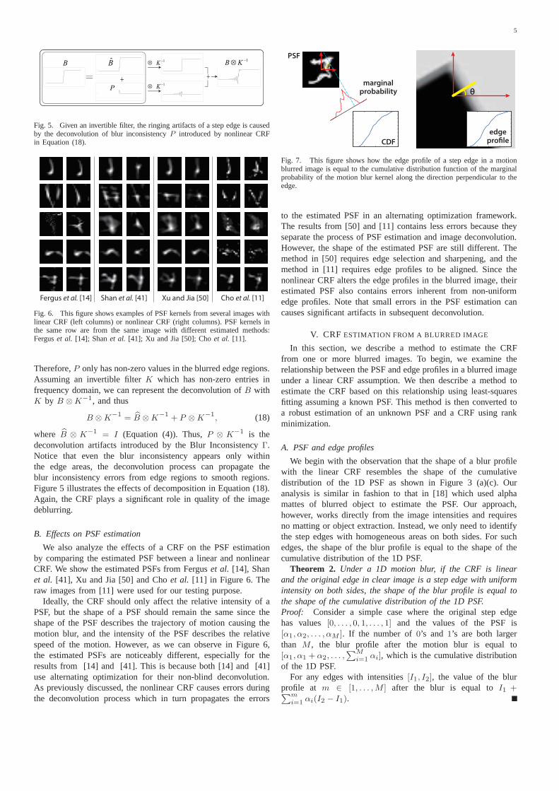
Fergus et al. [14] Shan et al. [41] Xu and Jia [50] Cho et al. [11]

Fig. 6. This figure shows examples of PSF kernels from several images withlinear CRF (left columns) or nonlinear CRF (right columns). PSF kernels inthe same row are from the same image with different estimated methods:Ferguset al. [14]; Shanet al. [41]; Xu and Jia [50]; Choet al. [11].

Therefore,P only has non-zero values in the blurred edge regions.Assuming an invertible filterK which has non-zero entries infrequency domain, we can represent the deconvolution ofB withK by B ⊗K−1, and thus

B ⊗K−1 = B ⊗K

−1 + P ⊗K−1

, (18)

where B ⊗ K−1 = I (Equation (4)). Thus,P ⊗ K−1 is thedeconvolution artifacts introduced by the Blur InconsistencyΓ.Notice that even the blur inconsistency appears only withinthe edge areas, the deconvolution process can propagate theblur inconsistency errors from edge regions to smooth regions.Figure 5 illustrates the effects of decomposition in Equation (18).Again, the CRF plays a significant role in quality of the imagedeblurring.

B. Effects on PSF estimation

We also analyze the effects of a CRF on the PSF estimationby comparing the estimated PSF between a linear and nonlinearCRF. We show the estimated PSFs from Ferguset al. [14], Shanet al. [41], Xu and Jia [50] and Choet al. [11] in Figure 6. Theraw images from [11] were used for our testing purpose.

Ideally, the CRF should only affect the relative intensity of aPSF, but the shape of a PSF should remain the same since theshape of the PSF describes the trajectory of motion causing themotion blur, and the intensity of the PSF describes the relativespeed of the motion. However, as we can observe in Figure 6,the estimated PSFs are noticeably different, especially for theresults from [14] and [41]. This is because both [14] and [41]use alternating optimization for their non-blind deconvolution.As previously discussed, the nonlinear CRF causes errors duringthe deconvolution process which in turn propagates the errors

θ

θ

PSF

marginalprobability

edgepro leCDF

Fig. 7. This figure shows how the edge profile of a step edge in a motionblurred image is equal to the cumulative distribution function of the marginalprobability of the motion blur kernel along the direction perpendicular to theedge.

to the estimated PSF in an alternating optimization framework.The results from [50] and [11] contains less errors because theyseparate the process of PSF estimation and image deconvolution.However, the shape of the estimated PSF are still different. Themethod in [50] requires edge selection and sharpening, and themethod in [11] requires edge profiles to be aligned. Since thenonlinear CRF alters the edge profiles in the blurred image, theirestimated PSF also contains errors inherent from non-uniformedge profiles. Note that small errors in the PSF estimation cancauses significant artifacts in subsequent deconvolution.

V. CRF ESTIMATION FROM A BLURRED IMAGE

In this section, we describe a method to estimate the CRFfrom one or more blurred images. To begin, we examine therelationship between the PSF and edge profiles in a blurred imageunder a linear CRF assumption. We then describe a method toestimate the CRF based on this relationship using least-squaresfitting assuming a known PSF. This method is then converted toa robust estimation of an unknown PSF and a CRF using rankminimization.

A. PSF and edge profiles

We begin with the observation that the shape of a blur profilewith the linear CRF resembles the shape of the cumulativedistribution of the 1D PSF as shown in Figure 3 (a)(c). Ouranalysis is similar in fashion to that in [18] which used alphamattes of blurred object to estimate the PSF. Our approach,however, works directly from the image intensities and requiresno matting or object extraction. Instead, we only need to identifythe step edges with homogeneous areas on both sides. For suchedges, the shape of the blur profile is equal to the shape of thecumulative distribution of the 1D PSF.

Theorem 2. Under a 1D motion blur, if the CRF is linearand the original edge in clear image is a step edge with uniformintensity on both sides, the shape of the blur profile is equal tothe shape of the cumulative distribution of the 1D PSF.Proof: Consider a simple case where the original step edgehas values[0, . . . , 0, 1, . . . , 1] and the values of the PSF is[α1, α2, . . . , αM ]. If the number of0’s and 1’s are both largerthan M , the blur profile after the motion blur is equal to[α1, α1 + α2, . . . ,

∑Mi=1 αi], which is the cumulative distribution

of the 1D PSF.For any edges with intensities[I1, I2], the value of the blur

profile at m ∈ [1, . . . ,M ] after the blur is equal toI1 +∑mi=1 αi(I2 − I1).

6

Theorem 2 is valid under the assumptions that the motionblurred image does not contain any noise or quantization error.

In the case of a 2D PSF, Theorem 2 still holds when the edgeis a straight line. In this case, the 1D PSF becomes the marginalprobability of the 2D PSF projected onto the line perpendicularto the edge direction as illustrated in Figure 7.

B. CRF approximation with a known PSF

Considering that the shape of blurred edge profiles are equal tothe shape of the cumulative distribution of the PSF2 if the CRFis linear. Given that we know the PSF, we can compute the CRFas follows:

argming(·)

E1∑

j=1

M∑

m=1

wj

(g(Ij(m))− lj

wj−

m∑

i=1

αi

)2

+

E2∑

j=1

M∑

m=1

wj

(g(Ij(m))− lj

wj−

M∑

i=m

αi

)2

, (19)

whereg(·) = f−1(·) is the inverse CRF function,E1 andE2 arethe numbers of selected blurred edge profiles from dark to brightregions and from bright region to dark regions, respectively.

The variableslj andwj are the minimum intensity value andthe intensity range (intensity difference between the maximumand the minimum intensity values) of the blurred edge profilesafter applying the inverse CRF. Blur profiles that span a widerintensity range are weighted more because their wider dynamicrange covers a larger portion ofg(·), and therefore provide moreinformation about the shape ofg(·). We filtered out the edgeswith wj < 0.1 since according to our blur inconsistency analysisin Section III, these low contrast edges does not provide muchinformation for PSF estimation.

We follow the method in [49] and model the inverse CRFg(·) using a polynomial of degreed = 5 with coefficientsap,i.e., g(I) =

∑dp=0 apI

p. The optimization is subject to boundaryconstraintsg(0) = 0 andg(1) = 1, and a monotonicity constraintthat enforces the first derivative ofg(·) to be non-negative. Ourgoal is to find the coefficientsap such that the following objectivefunction is minimized:

argminap

E1∑

j=1

M∑

m=1

wj

(∑dp=0 apIj(m)p − lj

wj−

m∑

i=1

αi

)2

+

E2∑

j=1

M∑

m=1

wj

(∑dp=0 apIj(m)p − lj

wj−

M∑

i=m

αi

)2

+λ1

a

20 +

(d∑

p=0

ap − 1

)2

+λ2

L∑

r=1

H

(d∑

p=0

ap

((r − 1

L

)p−(r

L

)p))

, (20)

whereH is the Heviside step function for enforcing the mono-tonicity constraint,i.e., H = 1 if g(r) < g(r − 1), or H = 0

otherwise andL is the maximum intensity level,e.g.255 for 8-bit color depth. The weights are fixed toλ1 = 100 and λ2 =

2For simplicity, we assume that the PSF is 1D, and it is well aligned with theedge orientation. If the PSF is 2D, we can compute the marginal probabilityof the PSF.

10, which control the boundary constraint and the monotonicconstraint, respectively. The solution of Equation (20) can beobtained by a simplex search method of Lagariaset al. [27]3.

C. CRF estimation with unknown PSF

Using the cumulative distribution of the PSF can reliablyestimate the CRF under ideal conditions. However, the PSF isusually unknown in practice. As we have studied in Section IV-B,nonlinear CRF affects the accuracy of the PSF estimation, whichin turn will affect our CRF estimation described in Section V-B.In this section, we introduce a CRF estimation method withoutexplicitly computing the PSF.

As previously discussed, we want to find an inverse responsefunction g(·) that makes the blurred edge profiles have the sameshape after applying the inverse CRF. This can be achieved byminimizing the distance between each blur profile to the averageblur profile:

argming(·)

E1∑

j=1

M∑

m=1

wj

(g(Ij(m))− lj

wj− A1(m)

)2

+

E2∑

j=1

M∑

m=1

wj

(g(Ij(m))− lj

wj− A2(m)

)2

, (21)

whereA1(m) =∑E1

k=1wk

W g(Ik(m)) is the weighted average blurprofile, andW =

∑E1

l=1 wl is a normalization factor.Using the constraint in Equation (21), we can compute the

CRF, however, this approach is unreliable not only because theconstraint in Equation (21) is weaker than the constraint inEquation (19), but the nature of least-squares fitting is sensitiveto outliers. To avoid these problems, we generalize our methodto robust estimation via rank minimization.

Recall that the edge profiles should have the same shape afterapplying the inverse CRF. This means that if the CRF is linear, theedge profiles are linearly dependent with each other, and hencethe observation matrix of edge profiles form a rank-1 matrix foreachgroup of edge profiles:

g(M)=

g(I1(1))− l1 · · · g(I1(M))− l1...

.. ....

g(IE1(1))− lE1

· · · g(IE1(M))− lE1

, (22)

whereM is length of edge profiles, andE1 is the number ofobserved edge profiles grouped according to the orientation ofedges. Now, we transform the problem into a rank minimizationproblem which finds a functiong(·) that minimizes the rank ofthe observation matrixM of edge profiles. Since the CRF is thesame for the whole image, we define our objective function forrank minimization as follow:

argming(·)

K∑

k=1

wkrank(g(Mk)), (23)

whereK is total number of observation matrix (total number ofgroup of edge profiles),wk is a weight given to each observationmatrix. We assign larger weight to the observation matrix thatcontains more edge profiles. Note that Equation (23) is alsoapplicable to multiple images since the observation matrix is builtindividually for each edge orientation and for each input image.

3fminsearch function in Matlab.

7

0 50 100 150 200 250 3000

1

PSF

0 50 100 150 200 250 3000

1

PSF

0 50 100 150 200 250 3000

1

PSF

0 50 100 150 200 250 3000

1

PSF

0 50 100 150 200 250 3000

1

PSF

(a) (b) (c) (d) (e)

0 0.2 0.4 0.6 0.8 10

0.1

0.2

0.3

0.4

0.5

0.6

0.7

0.8

0.9

1

Ground Truth

With Observation Matrix (Eq. 6) &

Rank Minimization (Eq. 10)

With known PSF (Eq. 4)

0 0.2 0.4 0.6 0.8 10

0.1

0.2

0.3

0.4

0.5

0.6

0.7

0.8

0.9

1

Ground Truth

With Observation Matrix (Eq. 6) &

Rank Minimization (Eq. 10)

With known PSF (Eq. 4)

0 0.2 0.4 0.6 0.8 10

0.1

0.2

0.3

0.4

0.5

0.6

0.7

0.8

0.9

1

Ground Truth

With Observation Matrix (Eq. 6) &

Rank Minimization (Eq. 10)

With known PSF (Eq. 4)

0 0.2 0.4 0.6 0.8 10

0.1

0.2

0.3

0.4

0.5

0.6

0.7

0.8

0.9

1

Ground Truth

With Observation Matrix (Eq. 6) &

Rank Minimization (Eq. 10)

With known PSF (Eq. 4)

0 0.2 0.4 0.6 0.8 10

0.1

0.2

0.3

0.4

0.5

0.6

0.7

0.8

0.9

1

Ground Truth

With Observation Matrix (Eq. 6) &

Rank Minimization (Eq. 10)

With known PSF (Eq. 4)

(f) (g) (h) (i) (j)

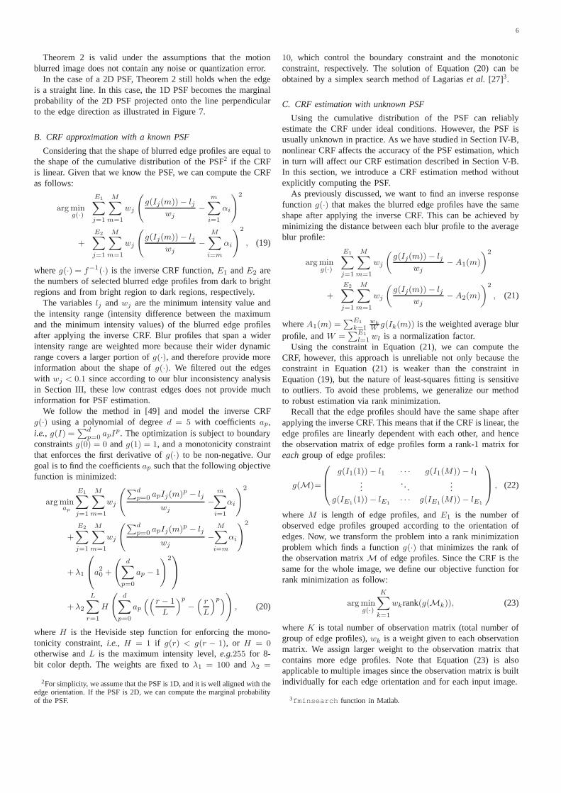
Fig. 8. We test the robustness of our CRF estimation method under different configurations. (a) Blur profiles with different intensity ranges, (b) edges in theoriginal image contains mixed intensities (edge width is equal to 3 pixels), (c) Gaussian noise (σ = 0.02) is added according to Equation (2), (d) the unionof intensity range of all blur profiles does not cover the whole CRF curve. (e) Blur profiles of (a), (b), (c), (d). The original image (black lines), the blurredimage with linear CRF (red lines), and the blurred image with nonlinear CRF (blue lines) are shown on top of each figure in (a)-(d). (f)-(i) the correspondingestimated inverse CRF using our methods with (a)-(d). (j) the corresponding estimated inverse CRF with multiple images in (e).

We evaluate the rank of matrixM by measuring the ratio ofits singular values:

argming(·)

K∑

k=1

wk

Ek∑

j=2

σkj

σk1, (24)

whereσkj are the singular values ofg(M)k. If the observationmatrix is rank-1, only the first singular values is nonzero andhence minimizes Equation (24). In our experiments, we foundthat Equation (24) can be simplified to just measuring the ratioof the first two singular values:

argming(·)

K∑

k=1

wkσk2σk1

. (25)

Combining the monotonic constraint, the boundary constraintand the polynomial function constraint from Equation (20), weobtain our final objective function:

argminap

K∑

k=1

wkσk2σk1

+ λ1

a

20 +

(d∑

p=0

ap − 1

)2 (26)

+λ2

L∑

r=1

H

(d∑

p=0

ap

((r − 1

L

)p−(r

L

)p))

.

Equation (26) can be solved effectively using nonlinear least-squares fitting4.

D. Implementation issues for 2D PSF

Our two proposed methods for CRF estimation are based on the1D blur profile analysis. Since, in practice, PSFs are 2D in nature,we need to group image edges with similar orientation and selectvalid edge samples for building the observation matrix. We usethe method in [11] to select the blurred edges. The work in [11]filtered edge candidates by keeping only high contrast straight-lineedges. A user parameter controls the minimum length of straight-line edges which depends on the size of the PSF. We refer to [11]

4lsqnonlin function in Matlab.

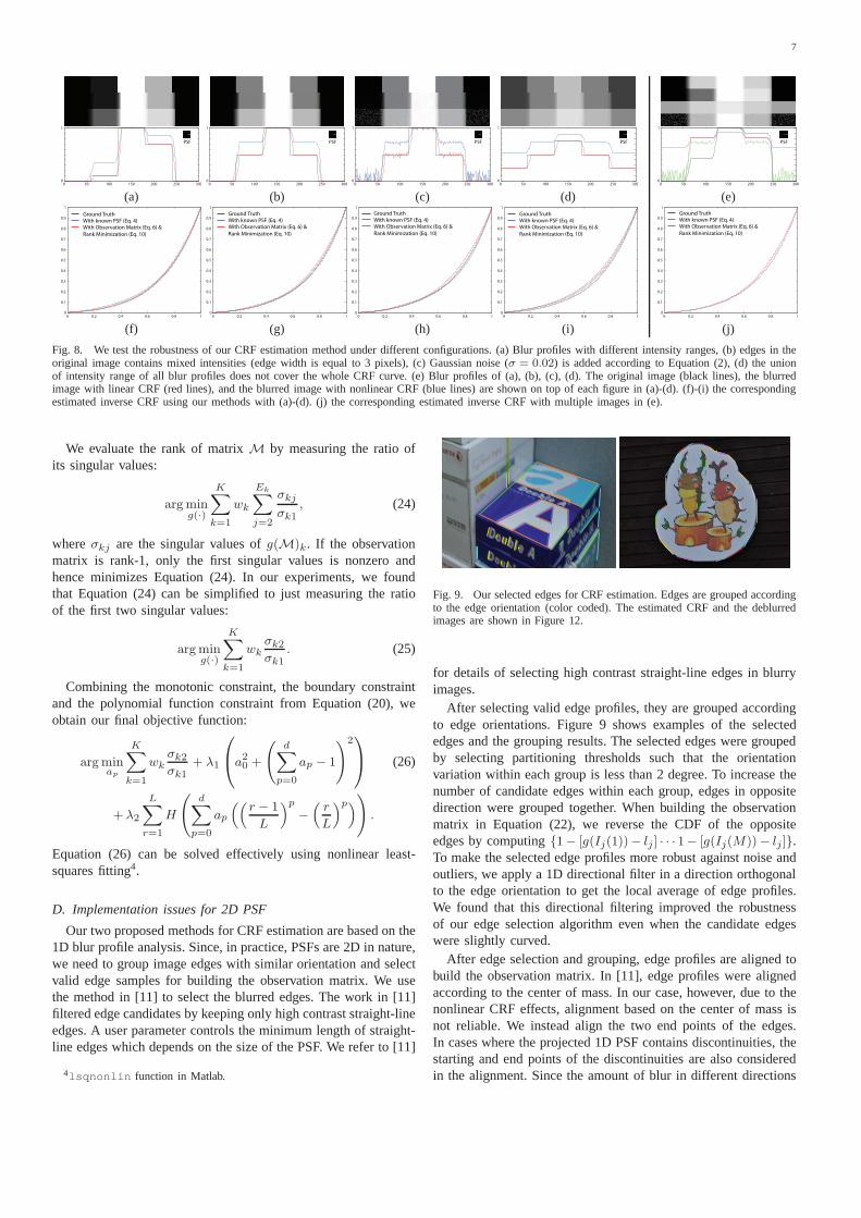
Fig. 9. Our selected edges for CRF estimation. Edges are grouped accordingto the edge orientation (color coded). The estimated CRF and the deblurredimages are shown in Figure 12.

for details of selecting high contrast straight-line edges in blurryimages.

After selecting valid edge profiles, they are grouped accordingto edge orientations. Figure 9 shows examples of the selectededges and the grouping results. The selected edges were groupedby selecting partitioning thresholds such that the orientationvariation within each group is less than 2 degree. To increase thenumber of candidate edges within each group, edges in oppositedirection were grouped together. When building the observationmatrix in Equation (22), we reverse the CDF of the oppositeedges by computing{1− [g(Ij(1))− lj ] · · · 1− [g(Ij(M))− lj ]}.To make the selected edge profiles more robust against noise andoutliers, we apply a 1D directional filter in a direction orthogonalto the edge orientation to get the local average of edge profiles.We found that this directional filtering improved the robustnessof our edge selection algorithm even when the candidate edgeswere slightly curved.

After edge selection and grouping, edge profiles are aligned tobuild the observation matrix. In [11], edge profiles were alignedaccording to the center of mass. In our case, however, due to thenonlinear CRF effects, alignment based on the center of mass isnot reliable. We instead align the two end points of the edges.In cases where the projected 1D PSF contains discontinuities, thestarting and end points of the discontinuities are also consideredin the alignment. Since the amount of blur in different directions

8

(a)

ISO: 100

T: 1/4 s

ISO: 100

T: 1/4 s

ISO: 3200

T: 1/80 s

ISO: 200

T: 1/5 s

(b)

0 0.2 0.4 0.6 0.8 10

0.2

0.4

0.6

0.8

1

image intensity

irra

dia

nce

Our estimated curveChart valuesCurve fitted by Chart valuesInverse Gamma−Correction

(d)

0 0.2 0.4 0.6 0.8 10

0.2

0.4

0.6

0.8

1

image intensity

irra

dia

nce

Our estimated curveChart valuesCurve fitted by Chart valuesInverse Gamma−Correction

(e)

0 0.2 0.4 0.6 0.8 10

0.2

0.4

0.6

0.8

1

image intensity

irra

dia

nce

Our estimated curveChart valuesCurve fitted by Chart valuesInverse Gamma−Correction

(f)

ISO: 3200

T: 1/125 s

ISO: 200

T: 1/10 s

(c)

Canon 400D Canon 60D Nikon D3100

Fig. 10. CRF estimation on real images. The top row shows the sharp/blurred pairs. The bottom row shows our recovered the CRF (in blue) and the groundtruth CRF (in red) obtained by acquiring the MacBeth’s chart (in green).

varies according to the shape of the PSF, we give a larger weightto the directions with longer edge profiles as they provide moreinformation about the CRF than sharp edges. When dealing withmultiple images, the same weighting scheme applies where alarger weight is given to a more blurry edge profile.

Our rank minimization using nonlinear least-squares fitting issensitive to the initial estimation of the CRF. In our implemen-tation, we use the average CRF profile from the database ofresponse functions (DoRF) created by Grossberg and Nayar [16]as our initial guess. The DoRF database contains 201 measuredfunctions which allows us to obtain a good local minima inpractice.

VI. EXPERIMENTAL RESULTS

In this section, we evaluate the performance of our CRFestimation method using both synthetic and real examples. Inthe synthetic examples, we test our algorithm under differentconditions in order to better understand the behaviors and thelimitations of our method. In the real examples, we evaluate ourmethod by comparing the amount of ringing artifacts with andwithout CRF intensity correction to demonstrate the effectivenessof our algorithm and the importance of CRF in the context ofimage deblurring.

A. Synthetic examples

Figure 8 shows the performance of our CRF estimation underdifferent conditions. We first test the effects of the intensity rangeof the blur profiles in Figure 8 (a). In a real application, it isuncommon that all edges will have a similar intensity range. These

intensity range variations can potentially affect the estimated CRFas low dynamic range edges usually contain larger quantizationerrors. As shown in Figure 8 (f), our method is reasonably robustto these intensity range variations.

Our method assumes that the original edges are step edges.In practice, there may be color mixing effect even for an edgethat is considered as a sharp edge. In our experiments, we findthat the performance of our approach degrades quickly if the stepedge assumption is violated. However, as shown in Figure 8 (g),our approach is still effective if the color mixing effects is lessthan 3 pixel wide given a PSF with size 15. The robustness ofour method when edge color mixing is present depends on thesize of the PSF with our approach being more effective for largerPSFs.

Noise is inevitable even when the ISO of a camera is high.We test the robustness of our method against image noise inFigure 8 (c). We add Gaussian noise to Equation (2) wherethe noise is added after the convolution process but before theCRF mapping. As can be observed in Figure 8 (h), the noiseaffects the accuracy of our method. In fact, using the model inEquation (2), we can observe that the noise has also capturedsome characteristics of the CRF. The magnitude of noise in thedarker region is larger than the magnitude of noise in the brighterregion. Such information may even be useful and combined intoour framework to improve the performance of our algorithm asdiscussed in [36].

We test the sensitivity of our algorithm when the union of blurprofiles does not cover the whole range of CRF. As can be seenin Figure 8 (i), our method still gives reasonable estimations. Thisis because the polynomial and monotonicity constraint assist in

9

Gamma 2.2Linear CRF Our CRF

[ Krishnan and Fergus NIPS 2009 ]

[ Levin et al. Siggraph 2007 ]

[ Xu and Jia ECCV 2010 ]

Ground Truth

Input

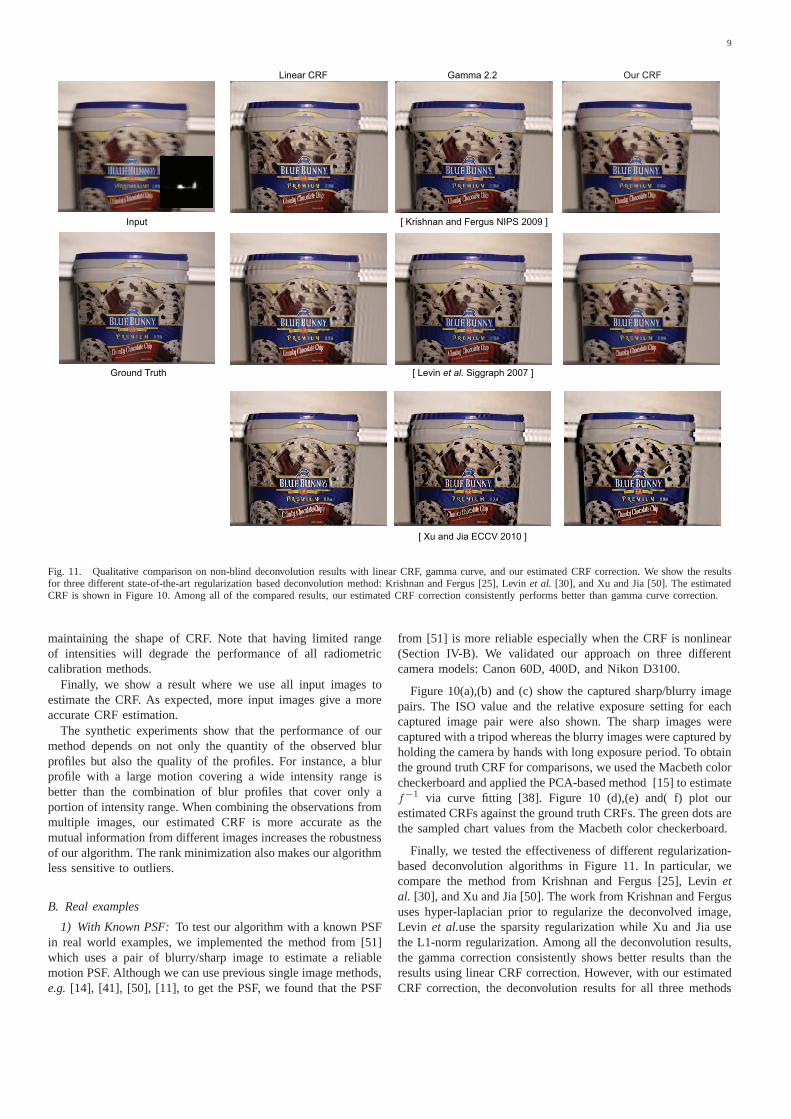
Fig. 11. Qualitative comparison on non-blind deconvolutionresults with linear CRF, gamma curve, and our estimated CRF correction. We show the resultsfor three different state-of-the-art regularization based deconvolution method: Krishnan and Fergus [25], Levinet al. [30], and Xu and Jia [50]. The estimatedCRF is shown in Figure 10. Among all of the compared results, our estimated CRF correction consistently performs better than gamma curve correction.

maintaining the shape of CRF. Note that having limited rangeof intensities will degrade the performance of all radiometriccalibration methods.

Finally, we show a result where we use all input images toestimate the CRF. As expected, more input images give a moreaccurate CRF estimation.

The synthetic experiments show that the performance of ourmethod depends on not only the quantity of the observed blurprofiles but also the quality of the profiles. For instance, a blurprofile with a large motion covering a wide intensity range isbetter than the combination of blur profiles that cover only aportion of intensity range. When combining the observations frommultiple images, our estimated CRF is more accurate as themutual information from different images increases the robustnessof our algorithm. The rank minimization also makes our algorithmless sensitive to outliers.

B. Real examples

1) With Known PSF:To test our algorithm with a known PSFin real world examples, we implemented the method from [51]which uses a pair of blurry/sharp image to estimate a reliablemotion PSF. Although we can use previous single image methods,e.g. [14], [41], [50], [11], to get the PSF, we found that the PSF

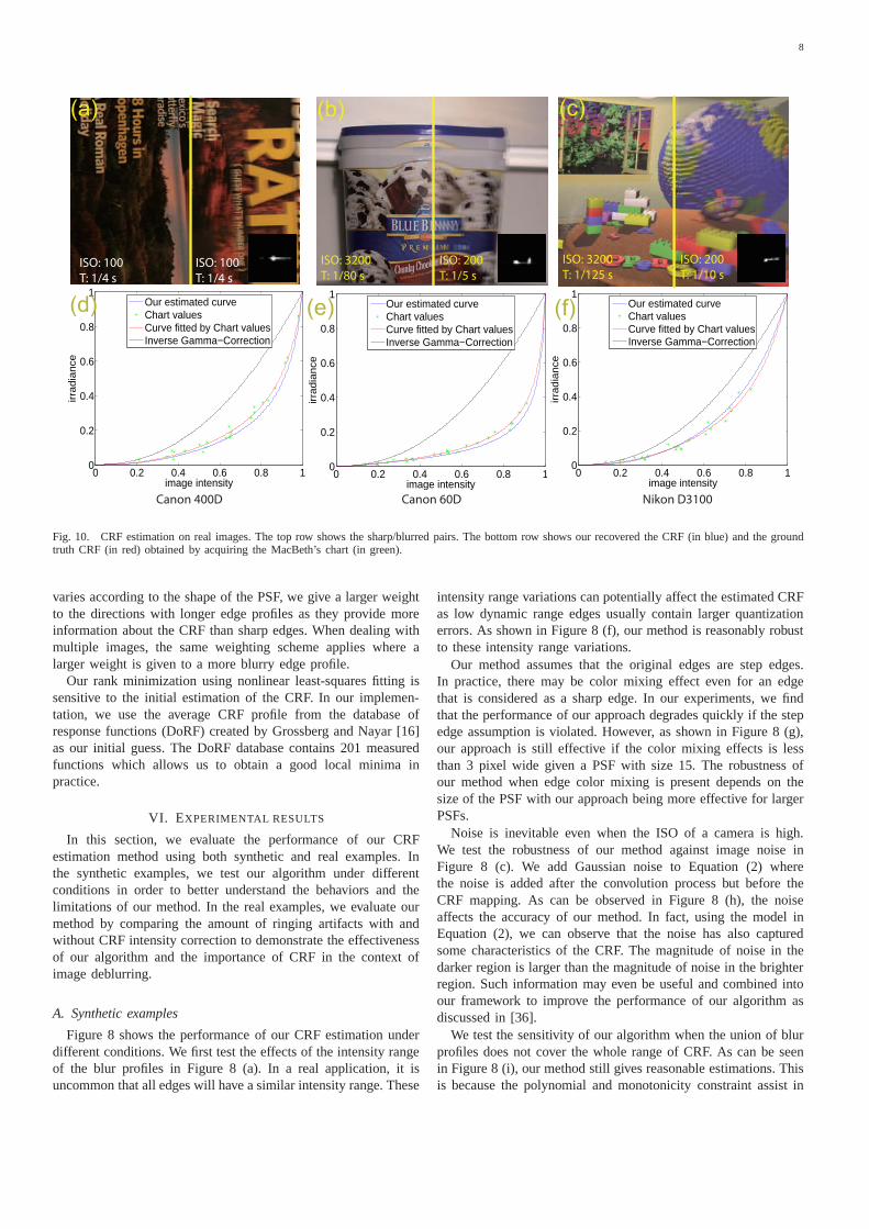
from [51] is more reliable especially when the CRF is nonlinear(Section IV-B). We validated our approach on three differentcamera models: Canon 60D, 400D, and Nikon D3100.

Figure 10(a),(b) and (c) show the captured sharp/blurry imagepairs. The ISO value and the relative exposure setting for eachcaptured image pair were also shown. The sharp images werecaptured with a tripod whereas the blurry images were captured byholding the camera by hands with long exposure period. To obtainthe ground truth CRF for comparisons, we used the Macbeth colorcheckerboard and applied the PCA-based method [15] to estimatef−1 via curve fitting [38]. Figure 10 (d),(e) and( f) plot ourestimated CRFs against the ground truth CRFs. The green dots arethe sampled chart values from the Macbeth color checkerboard.

Finally, we tested the effectiveness of different regularization-based deconvolution algorithms in Figure 11. In particular, wecompare the method from Krishnan and Fergus [25], Levinetal. [30], and Xu and Jia [50]. The work from Krishnan and Fergususes hyper-laplacian prior to regularize the deconvolved image,Levin et al.use the sparsity regularization while Xu and Jia usethe L1-norm regularization. Among all the deconvolution results,the gamma correction consistently shows better results than theresults using linear CRF correction. However, with our estimatedCRF correction, the deconvolution results for all three methods

10

0 0.2 0.4 0.6 0.8 10

0.1

0.2

0.3

0.4

0.5

0.6

0.7

0.8

0.9

1

Our Estimated CRF

with Single Image

Our Estimated CRF

with multiple Images

Inverse Gamma-Correction

Ground Truth

0 0.2 0.4 0.6 0.8 10

0.1

0.2

0.3

0.4

0.5

0.6

0.7

0.8

0.9

1

Our Estimated CRF

with Single Image

Our Estimated CRF

with multiple Images

Ground Truth

Inverse Gamma-Correction

0 0.2 0.4 0.6 0.8 10

0.1

0.2

0.3

0.4

0.5

0.6

0.7

0.8

0.9

1

Our Estimated CRF

with Single Image

Our Estimated CRF

with multiple Images

Ground Truth

Inverse Gamma-Correction

0 0.2 0.4 0.6 0.8 10

0.1

0.2

0.3

0.4

0.5

0.6

0.7

0.8

0.9

1

Our Estimated CRF

with Single Image

Our Estimated CRF

with multiple Images

Inverse Gamma-Correction

Ground Truth

(a) (b) (c) (d)

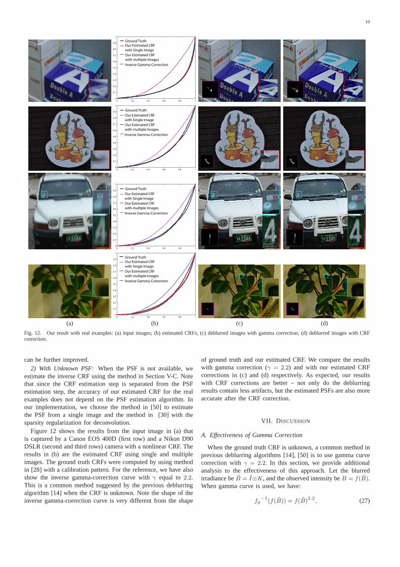
Fig. 12. Our result with real examples: (a) input images; (b) estimated CRFs; (c) deblurred images with gamma correction; (d) deblurred images with CRFcorrection.

can be further improved.2) With Unknown PSF:When the PSF is not available, we

estimate the inverse CRF using the method in Section V-C. Notethat since the CRF estimation step is separated from the PSFestimation step, the accuracy of our estimated CRF for the realexamples does not depend on the PSF estimation algorithm. Inour implementation, we choose the method in [50] to estimatethe PSF from a single image and the method in [30] with thesparsity regularization for deconvolution.

Figure 12 shows the results from the input image in (a) thatis captured by a Canon EOS 400D (first row) and a Nikon D90DSLR (second and third rows) camera with a nonlinear CRF. Theresults in (b) are the estimated CRF using single and multipleimages. The ground truth CRFs were computed by using methodin [28] with a calibration pattern. For the reference, we have alsoshow the inverse gamma-correction curve withγ equal to2.2.This is a common method suggested by the previous deblurringalgorithm [14] when the CRF is unknown. Note the shape of theinverse gamma-correction curve is very different from the shape

of ground truth and our estimated CRF. We compare the resultswith gamma correction (γ = 2.2) and with our estimated CRFcorrections in (c) and (d) respectively. As expected, our resultswith CRF corrections are better – not only do the deblurringresults contain less artifacts, but the estimated PSFs are also moreaccurate after the CRF correction.

VII. D ISCUSSION

A. Effectiveness of Gamma Correction

When the ground truth CRF is unknown, a common method inprevious deblurring algorithms [14], [50] is to use gamma curvecorrection withγ = 2.2. In this section, we provide additionalanalysis to the effectiveness of this approach. Let the blurredirradiance beB = I⊗K, and the observed intensity beB = f(B).When gamma curve is used, we have:

fg−1(f(B)) = f(B)2.2, (27)

11

0 0.2 0.4 0.6 0.8 10

0.1

0.2

0.3

0.4

0.5

0.6

0.7

0 0.2 0.4 0.6 0.8 10

0.1

0.2

0.3

0.4

0.5

0.6

0.7

(a) (b)

Fig. 13. The error curves of DoRF CRFs when (a) gamma curve (γ = 2.2)and (b) linear CRF are used to approximate the ground truth CRFs. Thehorizontal axis denotes theB values, and the vertical axis denotes the errorτ(B). The colors of these curves represent different underlying CRFs. Thecentral dark curve shows the meanτ for all the 188 real CRFs.

0 100 200 300 400 5000

0.2

0.4

0.6

0.8

1

0 100 200 300 400 500−0.2

0

0.2

0.4

0.6

0.8

1

1.2

0 100 200 300 400 500−0.2

0

0.2

0.4

0.6

0.8

1

1.2

0 100 200 300 400 500−0.2

0

0.2

0.4

0.6

0.8

1

1.2

0 100 200 300 400 5000

0.2

0.4

0.6

0.8

1

0 100 200 300 400 500−0.2

0

0.2

0.4

0.6

0.8

1

1.2

(a) (b) (c)

Fig. 14. We tested the effectiveness of gamma correction on synthetic exam-ple. (a) Input synthetic signal. Deconvolution with gamma curve correctionusing (b) wiener filter, and (c) sparsity regularization [30]. As discussed inSection IV, the ringing artifacts are mainly caused by the blur inconsistency.The gamma curve correction cannot fully eliminate blur inconsistency espe-cially for edges with high contrast.

wherefg(x) = x1/2.2 denotes the gamma curve CRF. Thus, theabsolute error introduced by the curve can be measured by:

τ (B) = |f(B)2.2 − B|. (28)

As discussed previously in Section III and Section IV, errors inthe CRF estimation will be directly transferred to the deblurredimage leading to large ringing artifacts that cannot fully besuppressed by regularization.

In order to show the magnitude of the approximation errors,we measure the differences between the gamma curve and the188 real CRF database [15] presented in Figure 2. Figure 13(a)shows the approximation errors of the gamma curve. The centraldark curve shown in the figure represents the mean of the errorτ (B) for all the 188 real CRF curves. Note that most part of theerror curves have errors larger than 0.1 which is10% of intensityrange. Some curves even have errors as large as0.6. For thereference, we also show the approximation errors if a linear CRFis used in Figure 13(b). Although the gamma curve has smallererrors compared to the linear CRF, gamma curve is insufficientto represent the real-world CRFs as noted in previous work [15],[31], [23].

Next, we use the synthetic examples in Figure 3 to analyzethe effectiveness of gamma curve correction in the non-blinddeconvolution. Figure 14 shows the result. The gamma curvecorrection can reduce errors compared to the results using the lin-

(a) Blurred image

(c) deblurred result with

gamma correction

(e) error map of (c)

(b) inverse CRFs

(f ) error map of (d)

0 0.2 0.4 0.6 0.8 10

0.2

0.4

0.6

0.8

1

Estimated curveGround truth curveGamma curve

(d) deblurred result with

our estimated CRF correction

Fig. 15. (a) Input blurred Image. (b) The inverse CRFs. Note the gammacurve with γ = 2.2 is closed to the inverse of mean CRFs. (c) Deblurredimage with gamma curve correction. (d) Deblurred image with our estimatedinverse CRF correction. (e) Error maps using gamma correction. (f) Errormaps using our estimated CRF correction.

ear correction, and the ringing artifacts are further reduced whena regularization-based deconvolution is used. Yet, as illustratedin Figure 14, it cannot completely remove the ringing artifactscaused by the blur inconsistency from nonlinear CRF.

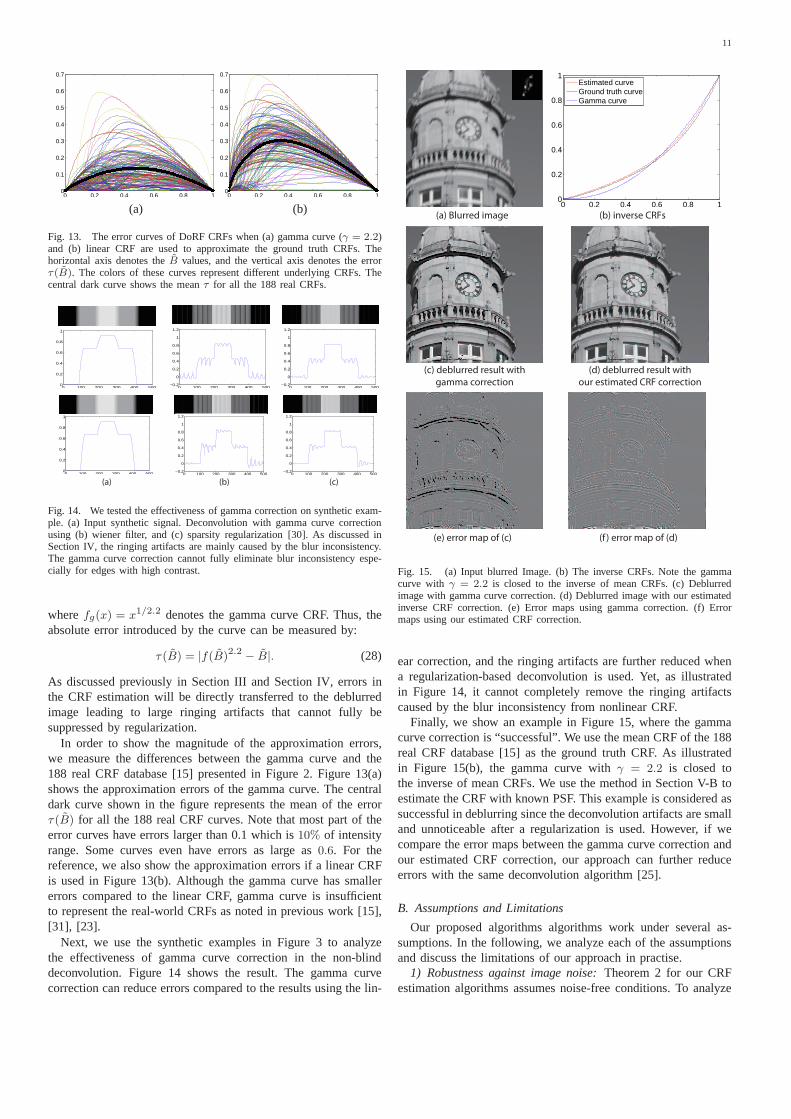
Finally, we show an example in Figure 15, where the gammacurve correction is “successful”. We use the mean CRF of the 188real CRF database [15] as the ground truth CRF. As illustratedin Figure 15(b), the gamma curve withγ = 2.2 is closed tothe inverse of mean CRFs. We use the method in Section V-B toestimate the CRF with known PSF. This example is considered assuccessful in deblurring since the deconvolution artifacts are smalland unnoticeable after a regularization is used. However, if wecompare the error maps between the gamma curve correction andour estimated CRF correction, our approach can further reduceerrors with the same deconvolution algorithm [25].

B. Assumptions and Limitations

Our proposed algorithms algorithms work under several as-sumptions. In the following, we analyze each of the assumptionsand discuss the limitations of our approach in practise.

1) Robustness against image noise:Theorem 2 for our CRFestimation algorithms assumes noise-free conditions. To analyze

12

0 0.2 0.4 0.6 0.8 10

0.2

0.4

0.6

0.8

1

Sigma 5Sigma 15Sigma 25Ground truth

0 0.2 0.4 0.6 0.8 10

0.2

0.4

0.6

0.8

1

Sigma 5Sigma 15Sigma 25Ground truth

0 5 10 15 20 250

0.005

0.01

0.015

0.02

noise variance (sigma)

RM

SE

of t

he e

stim

ated

CR

F

Canon400D CRFNikonD3100 CRF

Fig. 16. The estimated CRF under different noise level. (a) Canon400D.(b) Nikon D3100. (c) Plot of RMSE of the estimated CRF against differentamount of noise.

0 0.2 0.4 0.6 0.8 10

0.2

0.4

0.6

0.8

1

Ground truthOursGamma 2.2

(a) Input (b) with gamma 2.2

(d) Estimated CRF

0 0.5 1

(e) error map of (b) (f ) error map of (c)

(c) with our CRF

Fig. 17. Failure case. Our algorithm fails to estimate accurate CRF whenthe intensity range of input image is narrow. Yet, the deblurred result is stillbetter than the gamma curve with less ringing artifacts.

the robustness of our algorithms against image noise, we generatea set of synthetic blurry and noisy images with different amount ofGaussian noise. The ground truth image in Figure 15 and the CRFcurves of Canon400D and Nikon D3100 were used to producethe synthetic inputs. Figure 16 shows the plot of RMSE of theestimated CRF (with unknown PSF) against different amount ofnoise. Our CRF estimation algorithm is robust to image noisethanks to the usage of rank minimization optimization and thedirectional filtering in the edge selection step.

2) Spatially varying blur: Our CRF estimation algorithmsassume spatially invariant motion blur. When facing spatiallyvarying motion blur or defocus blur with different depth layers,the blind CRF estimation algorithm with unknown PSF will breakdown since the observation matrix is no longer a rank-1 matrix.In such scenario, only the CRF estimation algorithm with knownPSF can be used providing that the local PSF can be obtainedaccurately. The blur inconsistency analysis, however, should stillhold which claims that the irradiance of the blurry image shouldbe linearized before deblurring in order to avoid ringing artifactscaused by non-linear CRF.

3) Failure Cases:We finally provide a failure case in Figure 17where the CRF estimation fails due to the narrow intensityrange of the input image. The estimated CRF deviates from theground truth CRF especially for the area that is not covered bythe intensity range of input image. However, when comparingdeblurring results using a gamma curve, our result is still betterwith less ringing artifacts. As discussed earlier, the goal ofthis paper is to provide a method to handle nonlinear CRF indeblurring problem when the ground truth CRF is not accessible.In some cases, even an incorrectly estimated CRF may produce

better deblurring results than not performing linearization at all.The blur inconsistency analysis in Section III assumes a convex

CRF. In practice, there are camera models where the CRF isnon-convex in shape especially for the blue channel. We testedour algorithms for non-convex CRF using synthetic examples.However, we found that our estimated CRFs for unknown PSF arenot as accurate as the convex cases. One possible explanation isthat the non-convex CRFs deviate enough from the mean CRF tocause the nonlinear least-squares fitting in the rank minimizationto converge to an incorrect local minima.

We have also tested our algorithms for highly textured im-ages where straight-line edges are very limited. Both algorithmsfailed since the edge detection algorithm fail to detect straight-line edges. We consider this is a fundamental limitation to ouralgorithms.

VIII. C ONCLUSION

This paper offers two contributions targeting image deblurringin the face of nonlinear CRFs. First, we have presented an analysison the role that nonlinear CRFs play in image deblurring. Weprove that the blur inconsistency introduced by nonlinear CRFcan caused notable ringing artifacts in the deconvolution processwhich cannot be completely ameliorated by image regularization.Such blur inconsistency is spatially varying and it depends onedge sharpness, edge intensity range, and image brightness. Wehave also demonstrated how the nonlinear CRF adversely affectsPSF estimation for several state-of-the-art techniques.

In Section V, we prove how the shape of edge projectionsresemble the cumulative distribution function of 1D PSFs forlinear CRFs. This theorem was used to formulate two CRFestimation strategies for when the motion blur PSF kernel isknown or not known. In the latter case, we show how rankminimization can be used to provide a robust estimation. Wedo note that our approach is sensitive to the quality of theselected blur profiles. The requirement of straight line sharp edgesalso places a limitation to our current solution. To this end, wehave also provided a multiple image solution in case a motionblurred image does not contains sufficient edge profiles for CRFestimation.

Experimental results in real examples demonstrated the impor-tance of intensity linearization in the context of image deblurring.In addition, we have analyzed the effectiveness of gamma curvecorrection which is commonly used in previous deblurring algo-rithms [14], [50]. The shape of gamma curve withγ = 2.2 is closeto the inverse of mean CRFs. Therefore, in most cases, gammacurve correction is more effective than linear CRFs. However,when compared to the results with our estimated CRF corrections,gamma curve correction is still insufficient especially when theCRF is largely deviate from the mean CRFs.

IX. A CKNOWLEDGEMENT

This work was funded in part by the National ResearchFoundation (NRF) of Korea (2012-0003359), Microsoft ResearchAsia under the KAIST-Microsoft Research Collaboration Center(KMCC), Natural Science Foundation (China) (Nos:61273258,61105001), the Committee of Science and Technology, Shanghai(No. 11530700200), National Science Foundation (US) undergrants IIS-CAREER-0845268 and IIS-RI-1016395, the Air ForceOffice of Science Research under the YIP Award, and the Singa-pore A*STAR PSF grant (Proj No. 1121202020).

13

REFERENCES

[1] M. Ben-Ezra and S. Nayar. Motion-based Motion Deblurring.IEEETrans. PAMI, 26(6):689–698, Jun 2004.

[2] J. Cai, H. Ji, C. Liu, and Z. Shen. Blind motion deblurring from a singleimage using sparse approximation. InCVPR, 2009.

[3] A. Chakrabarti, D. Scharstein, and T. Zickler. ”an empirical cameramodel for internet color vision”. InBMCV, 2009.

[4] Y. Chang and J. Reid. Rgb calibration for color image-analysis inmachine vision.IEEE Trans. Image Processing, 5(10):14141422, 1996.

[5] J. Chen and C. K. Tang. Robust dual motion deblurring. InCVPR,2008.

[6] X. Chen, X. He, J. Yang, and Q. Wu. An effective document imagedeblurring algorithm. InCVPR, 2011.

[7] X. Chen, F. Li, J. Yang, and J. Yu. A theoretical analysis of cameraresponse functions in image deblurring. InECCV, 2012.

[8] S. Cho and S. Lee. Fast motion deblurring. InACM SIGGRAPH ASIA,2009.

[9] S. Cho, Y. Matsushita, and S. Lee. Removing non-uniform motion blurfrom images. InICCV, 2007.

[10] S. Cho, J. Wang, and S. Lee. Handling Outliers in Non-blind ImageDeconvolution. InICCV, 2011.

[11] T.-S. Cho, S. Paris, B. Freeman, and B. Horn. Blur kernel estimationusing the radon transform. InCVPR, 2011.

[12] P. Debevec and J. Malik. Recovering high dynamic range radiance mapsfrom photographs. InACM SIGGRAPH, 1997.

[13] H. Farid. Blind inverse gamma correction.IEEE Trans. ImageProcessing, 10(10):14281433, 2001.

[14] R. Fergus, B. Singh, A. Hertzmann, S. T. Roweis, and W. T. Freeman.Removing camera shake from a single photograph.ACM Trans. Graph.,25(3), 2006.

[15] M. Grossberg and S. Nayar. Modeling the space of camera responsefunctions. IEEE Trans. PAMI, 26(10), 2004.

[16] M. D. Grossberg and S. K. Nayar. What is the space of camera responsefunctions? InCVPR, 2003.

[17] M. Hirsch, C. Schuler, S. Harmeling, and B. Scholkopf. Fast removalof non-uniform camera shake. InICCV, 2011.

[18] J. Jia. Single image motion deblurring using transparency. InCVPR,2007.

[19] N. Joshi, S. Kang, L. Zitnick, and R. Szeliski. Image deblurring withinertial measurement sensors.ACM Trans. Graph., 29(3), 2010.

[20] N. Joshi, R. Szeliski, and D. Kriegman. Psf estimation using sharp edgeprediction. InCVPR, 2008.

[21] S. Kim, J. Frahm, and M. Pollefeys. Radiometric calibration withillumination change for outdoor scene analysis. InCVPR, 2008.

[22] S. Kim, Y.-W. Tai, S. Kim, M. S. Brown, and Y. Matsushita. Nonlinearcamera response functions and image deblurring. InCVPR, 2012.

[23] S. J. Kim, H. T. Lin, Z. Lu, S. Susstrunk, S. Lin, and M. S. Brown. A newin-camera imaging model for color computer vision and its application.In IEEE Trans. PAMI, 2012.

[24] S. J. Kim and M. Pollefeys. Robust radiometric calibration andvignetting correction.IEEE Trans. PAMI, 30(4), 2008.

[25] D. Krishnan and R. Fergus. Fast image deconvolution using hyper-laplacian priors. InNIPS, 2009.

[26] D. Krishnan, T. Tay, and R. Fergus. Blind deconvolution using anormalized sparsity measure. InCVPR, 2011.

[27] J. Lagarias, J. Reeds, M. Wright, and P. Wright. Convergence propertiesof the nelder-mead simplex method in low dimensions.SIAM Journalof Optimization, 9(1):112–147, 1998.

[28] J.-Y. Lee, B. Shi, Y. Matsushita, I. Kweon, and K. Ikeuchi. Radiometriccalibration by transform invariant low-rank structure. InCVPR, 2011.

[29] A. Levin. Blind motion deblurring using image statistics. InNIPS, 2006.[30] A. Levin, R. Fergus, F. Durand, and W. T. Freeman. Image and depth

from a conventional camera with a coded aperture.ACM Trans. Graph.,26(3), 2007.

[31] H. Lin, S. J. Kim, S. Susstrunk, and M. S. Brown. Revisiting radiometriccalibration for color computer vision. InICCV, 2011.

[32] S. Lin, J. Gu, S. Yamazaki, and H.-Y. Shum. Radiometric calibrationfrom a single image. InCVPR, 2004.

[33] S. Lin and L. Zhang. Determining the radiometric response functionfrom a single grayscale image. InCVPR, 2005.

[34] P.-Y. Lu, T.-H. Huang, M.-S. Wu, Y.-T. Cheng, and Y.-Y. Chuang. Highdynamic range image reconstruction from hand-held cameras. InCVPR,2009.

[35] L. Lucy. An iterative technique for the rectification of observeddistributions. Astron. J., 79, 1974.

[36] Y. Matsushita and S. Lin. Radiometric calibration from noise distribu-tions. In CVPR, 2007.

[37] T. Mitsunaga and S. Nayer. Radiometric self calibration. InCVPR,1999.

[38] T.-T. Ng, S.-F. Chang, and M.-P. Tsui. Using geometry invariants forcamera response function estimation. InCVPR, 2007.

[39] A. Rav-Acha and S. Peleg. Two motion blurred images are better thanone. PRL, 26:311–317, 2005.

[40] W. Richardson. Bayesian-based iterative method of image restoration.J. Opt. Soc. Am., 62(1), 1972.

[41] Q. Shan, J. Jia, and A. Agarwala. High-quality motion deblurring froma single image.ACM Trans. Graph., 2008.

[42] Y.-W. Tai, H. Du, M. Brown, and S. Lin. Image/video deblurring usinga hybrid camera. InCVPR, 2008.

[43] Y.-W. Tai, H. Du, M. S. Brown, and S. Lin. Correction of spatiallyvarying image and video motion blur using a hybrid camera.IEEETrans. PAMI, 32(6):1012–1028, 2010.

[44] Y.-W. Tai, N. Kong, S. Lin, and S. Shin. Coded exposure imaging forprojective motion deblurring. InCVPR, 2010.

[45] Y.-W. Tai and S. Lin. Motion-aware noise filtering for deblurring ofnoisy and blurry images. InCVPR, 2012.

[46] Y.-W. Tai, P. Tan, and M. Brown. Richardson-lucy deblurring for scenesunder projective motion path.IEEE Trans. PAMI, 33(8):1603–1618,2011.

[47] O. Whyte, J. Sivic, A. Zisserman, and J. Ponce. Non-uniform deblurringfor shaken images. InCVPR, 2010.

[48] N. Wiener. Extrapolation, interpolation, and smoothing of stationarytime series.New York: Wiley, 1949.

[49] B. Wilburn, H. Xu, and Y. Matsushita. Radiometric calibration usingtemporal irradiance mixtures. InCVPR, 2008.

[50] L. Xu and J. Jia. Two-phase kernel estimation for robust motiondeblurring. InECCV, 2010.

[51] L. Yuan, J. Sun, L. Quan, and H. Shum. Image deblurring withblurred/noisy image pairs.ACM Trans. Graph., 26(3), 2007.

Yu-Wing Tai received the BEng (first class hon-ors) and MS degrees in compute science from theHong Kong University of Science and Technology(HKUST) in 2003 and 2005 respectively, and thePhD degree from the National University of Sin-gapore (NUS) in June 2009. He joined the Ko-rea Advanced Institute of Science and Technology(KAIST) as an assistant professor in Fall 2009. Heregularly serves on the program committees for themajor Computer Vision conferences (ICCV, CVPR,and ECCV). His research interests include computer

vision and image/video processing. He is a member of the IEEE.

Xiaogang Chenis currently a PhD student in the In-stitute of Image Processing and Pattern Recognition,Shanghai Jiao Tong University. His research interestsinclude image and video processing, and computervision. He is a student member of the IEEE.

Sunyeong Kim received the BS and MS degrees inComputer Science from Korea Advanced Instituteof Science and Technology (KAIST) in 2010 and2012 respectively. She is currently pursuing the PhDdegree in KAIST. Her research interests includecomputer vision and image/video processing, espe-cially in computational photography. She is a studentmember of the IEEE.

14

Seon Joo Kimreceived the BS and MS degrees fromYonsei University, Seoul, Korea, in 1997 and 2001.He received the PhD degree in computer sciencefrom the University of North Carolina at ChapelHill in 2008. He is an assistant professor at theDepartment of Computer Science, Yonsei Universitysince March 2013. His research interests includecomputer vision, computer graphics/computationalphotography, and HCI/visualization. He is a memberof the IEEE.

Feng Li received his BE from the Departmentof Electrical Engineering, Fuzhou University, in2003, MS from the Institute of Pattern Recogni-tion, Shanghai Jiaotong University, in 2006, andhis PhD from the Department of Computer andInformation Sciences, University of Delaware, in2011. He joined Mitsubishi Electric Research Labsas a visiting research scientist in November 2011.His research interests include multi-camera systemdesign and applications, fluid surface reconstructionand medical imaging. He is a member of the IEEE.

Jie Yang received his PhD in computer science fromthe University of Hamburg, Germany. He is nowa professor and director of the Institute of ImageProcessing and Pattern Recognition, Shanghai JiaoTong University. He has led more than 30 nationaland ministry scientific research projects in imageprocessing, pattern recognition, data amalgamation,data mining, and artificial intelligence.

Jingyi Yu is an Associate Professor in the Depart-ment of Computer& Information Sciences and theDepartment of Electrical& Computer Engineeringat the University of Delaware. He received his B.S.from Caltech in 2000 and Ph.D. from MIT in 2005.His research interests span a range of topics in com-puter vision and computer graphics, especially oncomputational cameras and displays. He has servedas a Program Chair of OMNIVIS 11, a GeneralChair of Projector-Camera Systems 08, and an Areaand Session Chair of ICCV 11. He is a recipient of

both the NSF CAREER Award and the AFOSR YIP Award.

Yasuyuki Matsushita received his B.S., M.S. andPh.D. degrees in EECS from the University of Tokyoin 1998, 2000, and 2003, respectively. He joinedMicrosoft Research Asia in April 2003. He is a LeadResearcher in Visual Computing Group. His areasof research are photometric methods in computervision. He is on the editorial board member of IEEETransactions on Pattern Analysis and Machine Intel-ligence (TPAMI), International Journal of ComputerVision (IJCV), IPSJ Journal of Computer Vision andApplications (CVA), The Visual Computer Journal,

and Encyclopedia of Computer Vision. He served/is serving as a Program Co-Chair of PSIVT 2010, 3DIMPVT 2011, and ACCV 2012. He is appointedas a Guest Associate Professor at Osaka University (April 2010-), VisitingAssociate Professor at National Institute of Informatics (April 2011-) andTohoku University (April 2012-), Japan. He is a senior member of IEEE.

Michael S. Brown obtained his BS and PhD inComputer Science from the University of Kentuckyin 1995 and 2001 respectively. He is currently anAssociate Professor and Assistant Dean (ExternalRelations) in the School of Computing at the Na-tional University of Singapore. Dr. Browns researchinterests include computer vision, image processingand computer graphics. He has served as an areachair for CVPR, ICCV, ECCV, and ACCV and iscurrently an associate editor for the IEEE Transac-tions on Pattern Analysis and Machine Intelligence

(TPAMI).