Embed Size (px)
Citation preview

1
ISABE-2007-1210
Numerical Simulation of the Distortion Generated by Crosswind Inlet Flows
Y.Colina, B.Aupoixb, J.F. Boussugea, P. Chanezc
aCERFACS, CFD Team, 42 Av. G. Coriolis, 31057 Toulouse Cedex, France bONERA DMAE, 2 Av. Edouard Belin, 31055 Toulouse, France
cSNECMA, Villaroche, 77550 Moissy-Cramayel, France
Abstract
The study is motivated by the need of engine designers to have a robust, accurate and efficient tool capable of simulating complex flows around and inside an isolated, or close to the ground, nacelle in a crosswind. The code has to compute both incompressible and transonic zones and consequently a low-speed preconditioning method is required. Such separated flows exhibit considerable hysteresis in the separation and reattachment processes into the intake. This phenomenon was successfully solved by using dual time stepping integration. Lastly, nine turbulence models frequently employed for aeronautical flows have been compared to assess their predictive accuracy in computing complex three-dimensional separated flows. The models considered are the algebraic model of Baldwin and Lomax; both basic and rotation-curvature corrected versions of the Spalart-Allmaras one-equation models; k-l and three different k-ω models; the nonlinear eddy-viscosity model of Wallin and Johansson; and the differential Reynolds stress model of Speziale, Sarkar and Gatski. It is found that the one-equation model of Spalart-Allmaras, the k-ω SST model of Menter and the model of Wallin are the only models able to predict separated flow at high subsonic engine mass flowrate. Nomenclature A Jacobian matrix of the convective flux c speed of sound D Jameson artificial dissipation flux F flux tensor f,g,h convective fluxes fv,gv,hv viscous fluxes IDC circumferential distortion index k turbulent kinetic energy M Mach number M is Isentropic Mach number M lim Limit Mach number
Mr Reference Mach number MFR global mass flowrate (kg/s) MFRloc local mass flowrate nradius number of crowns P fan plane average pressure (Pa) Pi average pressure on i-th crown (Pa) Ri i-th crown radius Si i-th crown section U Euler symmetrizing variables vector W state vector in conservative variables β Mr scaling factor δ Weiss-Smith parameter ε Preconditioning parameter ΓW generic preconditioner in conservative form Γ preconditioner in Euler symmetrizing form γ specific-heat ratio ρ density σpgr pressure gradient free parameter ω specific turbulent dissipation Introduction
Nacelles design must fulfill geometrical constraints and engine requirements. One of the engine requirements is focused notably on the homogeneity of the flow in front of the fan which is quantified by the distortion levels of the total pressure in this plane. Airplane on the ground with crosswind is a critical case for the nacelle design. Subsonic or supersonic separations occur in the inlet, according to the engine mass flowrate. The resulting heterogeneity of the flow may account for the outbreak of aerodynamic instabilities of the fan blades and, if the distortion is large enough, the fan might stall. CERFACS, in collaboration with Snecma and ONERA, is working on the numerical simulation of such inlet flows with crosswind in order to predict distortion levels. Such crosswind flows exhibit three distinctive features challenging from a numerical and a modelling point of view.
Firstly, this application is featured by the cohabitation of incompressible and transonic areas

2
around the inlet lip. Indeed the infinite crosswind velocity varies between 15 and 30 kt which yield Mach numbers of the order of 10-2 whereas the Mach number may be superior to unity at the inlet lip. It turns out that the convergence of the pseudo-unsteady methods applied to the system of the Euler or Navier- Stokes equations in compressible flow is degraded at low velocities. This performance loss is due to the large disparity between the fast acoustic modes and the slow convective modes. Local preconditioning procedures [1-5] in which the time derivatives of the compressible equations are altered to control the eigenvalues and to accelerate convergence have been used.
The second flow feature of this application is the considerable hysteresis phenomenon occurring in the separation and reattachment processes as the engine mass flowrate evolves in the subsonic range. This behaviour has been experimentally highlighted by Raynal [6] or Quémard et al. [7]. They indicate that large hysteresis can be observed when testing model intakes by varying angle of attack. Recently, Hall and Hynes [8] carefully measured the hysteresis associated with separation and reattachment and showed that it is particularly sensitive to fan operating point and the location of the ground plane. At present there are few theoretical bases for analyzing aerodynamic hysteresis and it remains a difficult phenomenon to examine numerically. This phenomenon has been successfully reproduced in this study by using dual time stepping integration.
Lastly, crosswind intake flows feature complex three-dimensional separations starting from the leading edge of the nacelle down to the fan. Fast and accurate computations are required by engineers in nacelle design context. Therefore computational predictions for such flows are obtained by solving the Reynolds-averaged Navier-Stokes (RANS) equations in combination with eddy-viscosity turbulence models and Reynolds stress models. Studies of the predictive capabilities of turbulence models for the computation of adverse-pressure-gradient flows are mainly conducted for two-dimensional separated flows. Therefore, nine models are considered to assess their efficiency in computing separated intake flows for different engine mass flowrates in the subsonic range. Spalart-Allmaras, k-ω BSL and SST by Menter are the only models considered to evaluate the fan distortion, caused by the intake shock wave in the supersonic range.
The present work thus aims to assess some numerical tools along with first- and second-order turbulence modelling to compute crosswind inlet flows at low-Mach numbers along with separation hysteresis phenomena.
The first two sections deal with the test case and the numerical method. Numerical techniques are briefly described such as local preconditioning for low Mach numbers, DTS time integration and boundary conditions. In a third part, the implementation of turbulence models in the code is briefly described. The three last sections present results of simulations of the subsonic and supersonic separations, along with the resulting total pressure distortion in the fan plane, which concludes on the efficiency of turbulence modelling. Part I: Problem description and experimental setup Experimental facility
In order to characterize the intake separation area and to quantify the heterogeneity of the flow in front of the fan plane, Snecma intensively used experimental tests. The experimental setup tested at the F1 ONERA Fauga wind tunnel is illustrated in Fig. 1. The nacelle is set vertically and different crosswind velocities (from 15 to 30 kts) are considered for the entire engine flowrate range
Steady total pressure probes are allocated in the fan plane on eight arms at five different radii illustrated in Fig. 2. The probe locations are summarized in Tab. 1 and give some information about the spatial evolution of pressure distribution. Distortion levels definition
The influence of the total pressure distortion is generally studied with the introduction of the circumferential distortion index (IDC) to characterize the heterogeneity of the flow. This coefficient is defined as
IDC =nradius−1
MAXi=1
(
0.5
[
(Pi − Pmini)
P+
(Pi+1 − Pmini+1)
P
])
(1)
where P is the average pressure and Pmini the minimal pressure of the i-th crown. This index is devoted to assess the effect of the intake flow on the stability of the fan and enables to define surge margin.
The experiment conducted by ONERA consists of measuring the distortion in the fan plane as the mass flowrate (MFR) increases. Then the evolution of the distortion in terms of the flowrate may be represented, as depicted in Fig. 3. At low MFR, subsonic separation takes place in the intake. As MFR increases, the separation extent tends to reduce but total pressure losses become higher, resulting in IDC increase. At intermediate MFR, the boundary

3
Fig. 1 Crosswind tests at the F1 ONERA Fauga wind tunnel.
R3
θ
R5 R4 R2 R1
Fig. 2 Distortion measuring system.
Crown i Si/Stot Ri/Rext
1 0.1 0.3162 2 0.3 0.5477 3 0.5 0.7071 4 0.7 0.8367 5 0.9 0.9487
Table 1 Location of the crowns
1500MFR/MFR
max (engine scale) in kg/s
0
0.05
0.1
0.15
0.2
0.25
0.3
IDC
max
(C
ircum
fere
ntia
l dis
tort
ion
inde
x)
Subsonic separation
Reattachment
Supersonic separationMFR increase
MFR decrease
Hysteresis region
25
34
48
1/3 2/3
Fig. 3 Evolution of IDC versus mass flowrate.
layer reattaches in the diffuser which leads to the IDC drop. The flow is homogeneous in front of the fan plane and this flowrate range defines the working range. Then, at high MFR, the flow becomes supersonic on the lip and brings about a shock wave associated with strong total pressure losses, which explains the sudden increase of the IDC coefficient. This shock wave may induce a separation of the boundary layer: the resulting high heterogeneity of the flow causes aerodynamic instabilities responsible for strong vibrations which can damage the fan blades or lead to surge. Part II: Governing equations and numerical methods Navier-Stokes equations
The governing equations are the unsteady compressible Navier-Stokes equations which describe the conservation of mass, momentum and energy of the flow field. In conservative form, they can be expressed in three-dimensional Cartesian coordinates (x,y,z) as:
∂W
∂t+ divF = 0
(2)
where is the flux tensor. f, g, h are the inviscid fluxes and fv, gv, hv are the viscous fluxes. For Reynolds-Averaged Navier-Stokes equations (RANS) the turbulent fluxes are modelled with classical eddy viscosity assumptions or assessed with second-order closure models. Flow solver
The code used to solve this system of equation is the elsA software developed by ONERA and CERFACS (Cambier [9]). This numerical code is a powerful tool to compute a wide category of aerodynamics problems, for turbomachinery, aircraft or automotive. It solves the compressible Navier-Stokes equations using a finite volume method with
F = (f − fv, g − gv, h − hv)

4
various spatial discretization schemes like Jameson’s central difference scheme [10], Roe’s scheme [11] or HLLC scheme [12]. elsA is used for design at Airbus and Snecma.
Low speed preconditioning techniques
Preconditioning techniques involve the alteration of the time-derivatives used in time-marching CFD methods with the primary objective of enhancing their convergence. The original motivation for the development of these techniques arose from the need to efficiently compute low speed compressible flows. At low Mach numbers, the performances of traditional time-marching algorithms suffer because of the wide disparity that exists between the particle and acoustic wave speeds. Preconditioning methods introduce artificial time-derivatives which alter the acoustic waves so that they travel at speeds that are comparable in magnitude to the particle waves. Thereby good convergence characteristics may be obtained at all speeds. The alteration of the propagation velocities is done by multiplying the time-derivative of Eq.(2) by a preconditioning matrix ΓW as follows:
ΓW
∂W
∂t+ divF = 0
(3)
A generic Weiss-Smith/Choi-Merkle preconditioner based on Merkle/Weiss workgroups [1,4,5] was implemented and validated in elsA. Using the Euler symmetrizing variables dU=[dp/ρc, du, dv, dw, dS], the preconditioner can be written as follows:
Γ =
1ε 0 0 0 δ
ρc
0 1 0 0 00 0 1 0 00 0 0 1 00 0 0 0 1
(4)
where ε is the preconditioning parameter and δ is a free parameter varying from 0 to 1. For δ=0, the preconditioner is the Weiss-Smith preconditioner, which is a member of Turkel’s family. The preconditioning parameter is initially defined as:
ε = Min(1, Max(M2lim, M2)) (5)
Where Mlim is set to 10-5 to prevent singularities at solid walls and the above formulation yields ε=1 for Mach numbers greater than one.
It turns out that the use of preconditioning techniques greatly reduces the robustness of the flow solver. Numerical test cases show that the preconditioning parameter ε is the critical factor
influencing robustness issues. The determination of ε is implemented as follows:
ε = Min(1, Max(M2lim, M2, σpgr
|∆p|
ρc2, βM2
r , M2is))
(6)
where the limiting factor is introduced to avoid large pressure fluctuations in the vicinity of stagnation points [13]. The limitation is suggested by Turkel [14] to reduce preconditioning for viscous-dominated flows in boundary layers. Such regions are indeed dominated by diffusion processes and the formulation (5) for ε may lead to too large time steps in this region. Mr is usually taken as the inflow Mach number so that ε becomes constant in the boundary layer region. β ≈ 3-5 depending up on mass flowrates. The problematic of this restriction is the prescription of the reference Mach number. For crosswind inlet flows, the boundary layer expands at very low Mach numbers whereas it develops at much higher Mach numbers in the intake. This is why a restriction based on isentropic Mach number has been introduced with
M2
is =2
γ − 1
[
(
pt∞
p
)γ−1
γ
− 1
]
(7)
Given the fact that the normal pressure gradient is zero in the boundary layer, Mis is pretty constant in this region and is equal to the Mach number at the boundary layer interface. Artificial dissipation models
The use of preconditioning does not only reduce the stiffness of the system of equations; it also improves accuracy at low speeds. Turkel et al. [15] showed that the loss of accuracy of the original convective schemes is due to an ill-conditioning of artificial dissipation fluxes which become extremely large for very low velocities. The modification of the fluxes required to take into account the new characteristics of the preconditioned system results in a well conditioned dissipation formulation and ensures reliable accuracy. In the present work, the scalar artificial dissipation of Jameson et al., Roe and HLLC schemes have been modified.
The artificial dissipation flux D of Jameson et al. consists of a blend of second- and fourth-order differences. Within the finite volume method D is defined at the interface i+1/2 as:
Di+1/2 = ǫ
(2)i+1/2(Wi+1 − Wi)
−ǫ(4)i+1/2(Wi+2 − 3Wi+1 + 3Wi − Wi−1)
(8)
The coefficients ε(2) and ε(4) are used to locally adapt the dissipative flux and are directionally scaled
σpgr|∆p|
ρc2
βM2r

5
by the scaling factor ri+1/2:
ε(2)i+1/2 = k(2) ri+1/2 νi+1/2
ε(4)i+1/2 = max(0 , k(4) ri+1/2 − ε
(2)i+1/2)
(9)
The scaling factor ri+1/2 is calculated as the average of the spectral radii at the cell face
ri+1/2 =1
2(λ(Γ−1
W A)Ii + λ(Γ−1
W A)Ii+1)
(10)
where λ(ΓW-1A) is the spectral radius of the
preconditioned Jacobian matrix. The order of magnitude of the factor ri+1/2 is now the flow velocity and not the speed of sound as in the original model. However, as explained above, the preconditioning parameter ε has been reduced in the boundary layer for stiffness issues, which may account for high values of artificial dissipation close to the wall. Thus the strategy consists of damping the artificial dissipation D near the wall by multiplying this flux by (M/Mis)
2. The modification of Roe and HLLC scheme
follows the procedure described in [16] and [17] respectively. Numerical studies showed that the use of such upwind schemes led to too much dissipative solutions, notably predicting reattachment mass flowrates which are much lower than the one inferred from experimental data. Numerical computations presented below are based on preconditioned Jameson scheme along with artificial dissipation damping.
Hysteresis simulation: unsteady time integration
As pointed out above, crosswind inlet flows exhibit considerable hysteresis in the separation and reattachment processes as the engine mass flowrate evolves. As illustrated in Fig. 3, when the flow is separated, increasing the mass flowrate tends to reduce the separated area, bringing the flowfield closer to reattachment. Once the flow is reattached, if the mass flowrate is reduced, separation occurs at a much lower flowrate than that required for reattachment. At present, theoretical bases for analyzing aerodynamic hysteresis are not well developed and it remains a difficult phenomenon to investigate numerically.
In our study, it turns out that steady computations failed to yield steady distortion in fan plane. Indeed these methods, involving local time stepping or preconditioning procedures alter time derivatives of the original equations. The loss of time consistency in the hysteresis region may account for the inefficiency of these methods.
On the contrary, unsteady time integration techniques such as Gear or Dual Time Stepping (DTS) methods were successful in converging to a
steady separated solution. Time marching algorithm for the inner loop is a backward Euler scheme with a 4 steps LU-SSOR decomposition. Fig. 4 shows the hysteresis phenomenon simulation realized with DTS time integration and the k-ω BSL model of Menter. The simulation is done by running a series of increasing MFR simulations until reattachment of the flow. Then a series of decreasing MFR simulations is done until separation of the flow. This technique enables to capture the two possible states of the flow field for a given flowrate.
Boundary conditions for nacelle flows
For powered nacelle simulations and to control the intake flow rate of the nacelle, two different options for specifying fan plane boundary conditions are implemented.
The first one is to specify the global mass flux MFR at the fan plane:
MFR =
∫
fan
ρ~q · ~ndS
(11)
where is the velocity vector. From this specified value, a local mass flux MFRloc may be calculated for each node of the fan plane by homothety:
MFRloc =
(
MFR
MFRsch
)
ρsch~q sch · ~n
(12)
where the superscript sch denotes the flow variables estimated by the numerical scheme. The integration of this equation over the fan plane surface clearly verifies Eq. (11). The advantage of this formulation is that it allows us to simulate a specific MFR and to compare it directly with experimental data. However, the lack of robustness of this condition, especially in the initial phase of a simulation, makes it difficult to use.
The second option is thus to specify the constant static pressure p at the fan face. This formulation is
1000MFR/MFR
max (engine scale) in kg/s
0
0.05
0.1
0.15
0.2
IDC
max
(C
ircum
fere
ntia
l dis
tort
ion
inde
x)
DTS integration-MFR increaseDTS integration-MFR decrease
Subsonic separation
Reattachment
Experiment-MFR increaseExperiment-MFR decrease
1/3 2/3
Fig. 4 Hysteresis simulation with DTS integration technique.
~q

6
more robust than the mass flux one; however some uncertainty remains to simulate a specific mass flowrate. Besides, this condition is dependent on the numerical scheme and model used, which yield different boundary layer thicknesses –thus different flow rates– for the same outlet static pressure.
Part III: Investigated models In the present study, we mainly focus on eddy-
viscosity transport models (EVMs). Indeed these models are presently very popular in computational fluid-dynamics applications. They have a major advantage in their simplicity and practical usability and constitute the aerospace industry’s “work horses”. However, some weaknesses are still unresolved with EVMs. Indeed, the Boussinesq hypothesis directly relates the turbulent shear stress to the mean velocity strain rate tensor. Therefore it cannot account for any history effects. It also assumes an isotropic character for the eddy viscosity and is unable to reproduce stress anisotropy [18]. These shortcomings may be particularly penalizing for highly separated flows. For such flows, normal tensions differ completely from those arising in an attached boundary layer. History effects strongly affect the turbulence and the mean strain rate relaxes very rapidly but not the Reynolds stresses. This is why Differential Reynolds Stress Models (DRSMs) may be attractive for such applications. They yield superior predictions of nonequilibrium flows and account for the effects of stress anisotropy, streamline curvature and flow rotation [19]. The weak point of the presently tested DRSM model is the wall region treatment, which diminishes the inherent superiority of DRSMs compared to EVMs.
A total of nine different models is considered. They range from the algebraic Baldwin-Lomax model [20] over the Baseline Spalart-Allmaras [21] (SA) and Spalart-Allmaras with rotation and curvature correction [22] one-equation models to the k-l model of Smith [23] and three different two-equation k-ω models (k-ω 1988 by Wilcox [24], k-ω BSL and SST by Menter [25]). In addition, the Speziale-Sarkar-Gatski (SSG) DRSM [27] along with the nonlinear explicit algebraic Reynolds-stress model (EARSM) proposed by Wallin and Johansson [26] are also investigated. We have not included a classical k-ε model in our study because its deficiencies for predicting aerodynamic flows with adverse pressure gradients are well known [29-30].
All models are applied in the version proposed by the referenced authors except for the EARSM of Wallin and Johansson and the DRSM models. The reader may refer to the cited literature for details of
Model Reference Baldwin-Lomax (BL) Spalart-Allmaras (SA) Spalart-Allmaras RC (SARC) k-l Smith k-ω 1988 by Wilcox k-ω BSL by Menter k-ω SST by Menter EARSM of Wallin and Johansson DRSM of Speziale, Sarkar and Gatski
[20] [21] [22] [23] [24] [25] [25]
[26,27] [28]
Table 2 Turbulence investigated models the models. Comments are made in the following about how models are implemented in elsA and used in this study.
The k-ω model of Wilcox corresponds to the 1988 version of the model. Zheng limiter has been applied to provide a lower bound for the specific dissipation ω and hence resolve the sensitivity of the k- ω model to the level of ω in the external flow.
The Wallin-Johansson model applies a non linear constitutive relation for computing the eddy viscosity consisting of functionals of Sij and Ωij. The version used here relies on the k-kL model developed at ONERA [27] for the computation of k and L, which are used to scale the terms in the constitutive relation. The main advantage of this model over the linear one is its ability to predict anisotropy of normal Reynolds stresses.
Lastly, the DRSM model considered is based on the SSG model (Speziale et al.), extended to the wall region by Chen et al. [31]. Chen et al. model uses a transport equation for the turbulent kinetic energy dissipation rate, which has been shown to degrade numerical stability. The specific dissipation equation Menter’s BSL model has been preferred. Moreover, the use of the specific dissipation is well known to improve predictions of flows submitted to positive pressure gradients. The complete model description can be found in the FLOMANIA book [32].
Part IV: Simulation of subsonic separation and reattachment
The configuration provided by Snecma consists of the Lara nacelle tested at the F1 ONERA wind tunnel. The computational domain, illustrated in Fig. 1, is designed to match the wind tunnel facilities. A crosswind velocity of 30 kt (corresponding to a Mach number of 0.04) and a Reynolds number of 4.5 106 are considered while an outflow condition is imposed downstream of the fan plane using a constant static pressure lower than the freestream one. The simulation is conducted by running a series of increasing MFR until reattachment of the flow.

7
Fig. 5 Partial view of the 3D Lara nacelle mesh. Fig. 6 2D cut in xOz plane.
Meshing strategy
The mesh is generated using ICEM-CFD software and a global view of the nacelle is represented in Fig. 5. Fig. 6 shows parts of the C-mesh around the nacelle, which is suitable to treat boundary layer separation. In order to avoid interaction of the separation in the intake with the boundary condition, the outlet condition is imposed far more inside the inlet than in the wind tunnel test.
The fine Euler mesh is a structured multi-block mesh with 32 blocks and contains about 3.5 million grid points. The viscous grid is generated by remeshing the Euler grid close to the walls such that the first cell height in wall unit, based upon the internal Reynolds number, is lower than unity. The simulation of a large range of flowrates leads to generate a specific viscous mesh for each MFR. Sensitivity study showed that at least 40 points are required in the wall normal direction resulting in a final viscous mesh with 5.2 million grid points.
Results and discussion
All the models listed on Table 2 have been tested on the Lara nacelle to assess their ability to predict accurate solution as the flow separates. The results are presented for two engine mass flowrates corresponding respectively to points 25 and 34 of the experiment as illustrated in Fig. 3. Firstly, wall isentropic Mach number distributions are computed at four angular positions 0o, 45o, 90o and 135o as illustrated in Fig. 7(a) for both external and internal flows. The crosswind direction follows the y-axis direction. Besides, total pressure drops are plotted in terms of the circumferential angle θ as described in Fig. 7(b) and yield details on the three-dimensional separation extent.
Figure 10 compares the models listed on table 2 at PT25, where a massive separation takes place as illustrated in Fig. 8. Fig. 10(b) shows that the separation extends from θ=0o to 180o, with quite weak pressure drops of about 5% which result in a
y
z
-0.2 0 0.2
-0.2
-0.1
0
0.1
0.2
Pi
0.720.710.700.690.690.680.670.660.650.640.640.630.620.61
R4R4
R3
R2
R1
Fig. 7 Repartition of the probes to extract (a) wall isentropic Mach and (b) fan plane total pressure distributions.
Fan plane location
0o
45o
90o
135o
(a) (b)
8
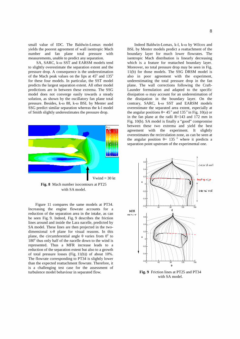
small value of IDC. The Baldwin-Lomax model yields the poorest agreement of wall isentropic Mach number and fan plane total pressure with measurements, unable to predict any separation.
SA, SARC, k-ω SST and EARSM models tend to slightly overestimate the separation extent and the pressure drop. A consequence is the underestimation of the Mach peak values on the lips at 45o and 135o for these four models. In particular, the SST model predicts the largest separation extent. All other model predictions are in between these extrema. The SSG model does not converge easily towards a steady solution, as shown by the oscillatory fan plane total pressure. Besides, k-ω 88, k-ω BSL by Menter and SSG predict similar separation whereas the k-l model of Smith slightly underestimates the pressure drop.
Figure 11 compares the same models at PT34. Increasing the engine flowrate accounts for a reduction of the separation area in the intake, as can be seen Fig. 9. Indeed, Fig. 9 describes the friction lines around and inside the Lara nacelle, predicted by SA model. These lines are then projected in the two-dimensional x-θ plane for visual reasons. In this plane, the circumferential angle θ varies from 0o to 180o thus only half of the nacelle down to the wind is represented. Thus a MFR increase leads to a reduction of the separation extent but also to a growth of total pressure losses (Fig. 11(b)) of about 10%. The flowrate corresponding to PT34 is slightly lower than the expected reattachment flowrate. Therefore, it is a challenging test case for the assessment of turbulence model behaviour in separated flow.
Indeed Baldwin-Lomax, k-l, k-ω by Wilcox and BSL by Menter models predict a reattachment of the boundary layer for much lower flowrates. The isentropic Mach distribution is linearly decreasing which is a feature for reattached boundary layer. Moreover, no total pressure drop may be seen in Fig. 11(b) for those models. The SSG DRSM model is also in poor agreement with the experiment, underestimating the total pressure drop in the fan plane. The wall corrections following the Craft-Launder formulation and adapted to the specific dissipation ω may account for an underestimation of the dissipation in the boundary layer. On the contrary, SARC, k-ω SST and EARSM models overestimate the separated area extent, especially at the angular positions θ= 45 o and 135 o in Fig. 10(a) or in the fan plane at the radii R=143 and 172 mm in Fig. 10(b). SA model is finally a “good” compromise between these two extrema and yield the best agreement with the experiment. It slightly overestimates the recirculation zone, as can be seen at the angular position θ= 135 o where it predicts a separation point upstream of the experimental one.
Fig. 9 Friction lines at PT25 and PT34
with SA model.
Fig. 8 Mach number isocontours at PT25 with SA model.
Vwind = 30 kt

9
-0.2 0 0.2x
0
0.1
0.2
0.3
0.4
0.5
Mis
Expe.BLk-lk-ω 88
0o
-0.2 0 0.2x
0
0.1
0.2
0.3
0.4
0.5
Mis
45o
-0.2 0 0.2x
0
0.1
0.2
0.3
0.4
0.5
Mis
90o
-0.2 0 0.2x
0
0.1
0.2
0.3
0.4
0.5
Mis
135o
0 90 180 270 360 θ
0.85
0.9
0.95
1
1.05
Pt
Expe.BLk-lk-ω 88
R = 92mm
0 90 180 270 360θ
0.85
0.9
0.95
1
1.05
Pt
R = 111mm
0 90 180 270 360θ
0.85
0.9
0.95
1
1.05
Pt
R = 143mmm
0 90 180 270 360θ
0.85
0.9
0.95
1
1.05
Pt
R = 172mm
-0.2 0 0.2x
0
0.1
0.2
0.3
0.4
0.5
Mis
Expe.SASARC
0o
-0.2 0 0.2x
0
0.1
0.2
0.3
0.4
0.5
Mis
45o
-0.2 0 0.2x
0
0.1
0.2
0.3
0.4
0.5
Mis
90o
-0.2 0 0.2x
0
0.1
0.2
0.3
0.4
0.5
Mis
135o
0 90 180 270 360 θ
0.85
0.9
0.95
1
1.05
Pt
Expe.SASARC
R = 92mm
0 90 180 270 360θ
0.85
0.9
0.95
1
1.05
Pt
R = 111mm
0 90 180 270 360θ
0.85
0.9
0.95
1
1.05
Pt
R = 143mmm
0 90 180 270 360θ
0.85
0.9
0.95
1
1.05
Pt
R = 172mm
-0.2 0 0.2x
0
0.1
0.2
0.3
0.4
0.5
Mis
Expe.Menter BSLMenter SST
0o
-0.2 0 0.2x
0
0.1
0.2
0.3
0.4
0.5
Mis
45o
-0.2 0 0.2x
0
0.1
0.2
0.3
0.4
0.5
Mis
90o
-0.2 0 0.2x
0
0.1
0.2
0.3
0.4
0.5
Mis
135o
0 90 180 270 360 θ
0.85
0.9
0.95
1
1.05
Pt
Expe.Menter BSLMenter SST
R = 92mm
0 90 180 270 360θ
0.85
0.9
0.95
1
1.05P
tR = 111mm
0 90 180 270 360θ
0.85
0.9
0.95
1
1.05
Pt
R = 143mmm
0 90 180 270 360θ
0.85
0.9
0.95
1
1.05
Pt
R = 172mm
-0.2 0 0.2x
0
0.1
0.2
0.3
0.4
0.5
Mis
Expe.DRSMEARSM
0o
-0.2 0 0.2x
0
0.1
0.2
0.3
0.4
0.5
Mis
45o
-0.2 0 0.2x
0
0.1
0.2
0.3
0.4
0.5
Mis
90o
-0.2 0 0.2x
0
0.1
0.2
0.3
0.4
0.5
Mis
135o
0 90 180 270 360 θ
0.85
0.9
0.95
1
1.05
Pt
Expe.DRSMEARSM
R = 92mm
0 90 180 270 360θ
0.85
0.9
0.95
1
1.05
Pt
R = 111mm
0 90 180 270 360θ
0.85
0.9
0.95
1
1.05
Pt
R = 143mmm
0 90 180 270 360θ
0.85
0.9
0.95
1
1.05
Pt
R = 172mm
(a) (b)
Fig. 10 Wall isentropic Mach (a) and fan plane total pressure (b) distributions at PT25.

10
-0.2 0 0.2x
0
0.2
0.4
0.6
0.8
1
Mis
Expe.BLk-lk-ω 88
0o
-0.2 0 0.2x
0
0.2
0.4
0.6
0.8
1
Mis
45o
-0.2 0 0.2x
0
0.2
0.4
0.6
0.8
1
Mis
90o
-0.2 0 0.2x
0
0.2
0.4
0.6
0.8
1
Mis
135o
0 90 180 270 360 θ
0.85
0.9
0.95
1
1.05
Pt
Expe.BLk-lk-ω 88
R = 92mm
0 90 180 270 360θ
0.85
0.9
0.95
1
1.05
Pt
R = 111mm
0 90 180 270 360θ
0.85
0.9
0.95
1
1.05
Pt
R = 143mmm
0 90 180 270 360θ
0.85
0.9
0.95
1
1.05
Pt
R = 172mm
-0.2 0 0.2x
0
0.2
0.4
0.6
0.8
1
Mis
Expe.SASARC
0o
-0.2 0 0.2x
0
0.2
0.4
0.6
0.8
1
Mis
45o
-0.2 0 0.2x
0
0.2
0.4
0.6
0.8
1
Mis
90o
-0.2 0 0.2x
0
0.2
0.4
0.6
0.8
1
Mis
135o
0 90 180 270 360 θ
0.85
0.9
0.95
1
1.05
Pt
Expe.SASARC
R = 92mm
0 90 180 270 360θ
0.85
0.9
0.95
1
1.05
Pt
R = 111mm
0 90 180 270 360θ
0.85
0.9
0.95
1
1.05
Pt
R = 143mmm
0 90 180 270 360θ
0.85
0.9
0.95
1
1.05
Pt
R = 172mm
-0.2 0 0.2x
0
0.2
0.4
0.6
0.8
1
Mis
Expe.Menter BSLMenter SST
0o
-0.2 0 0.2x
0
0.2
0.4
0.6
0.8
1
Mis
45o
-0.2 0 0.2x
0
0.2
0.4
0.6
0.8
1
Mis
90o
-0.2 0 0.2x
0
0.2
0.4
0.6
0.8
1
Mis
135o
0 90 180 270 360 θ
0.85
0.9
0.95
1
1.05
Pt
Expe.Menter BSLMenter SST
R = 92mm
0 90 180 270 360θ
0.85
0.9
0.95
1
1.05P
t
R = 111mm
0 90 180 270 360θ
0.85
0.9
0.95
1
1.05
Pt
R = 143mmm
0 90 180 270 360θ
0.85
0.9
0.95
1
1.05
Pt
R = 172mm
-0.2 0 0.2x
0
0.2
0.4
0.6
0.8
1
Mis
Expe.DRSMEARSM
0o
-0.2 0 0.2x
0
0.2
0.4
0.6
0.8
1
Mis
45o
-0.2 0 0.2x
0
0.2
0.4
0.6
0.8
1
Mis
90o
-0.2 0 0.2x
0
0.2
0.4
0.6
0.8
1
Mis
135o
0 90 180 270 360 θ
0.85
0.9
0.95
1
1.05
Pt
Expe.DRSMEARSM
R = 92mm
0 90 180 270 360θ
0.85
0.9
0.95
1
1.05
Pt
R = 111mm
0 90 180 270 360θ
0.85
0.9
0.95
1
1.05
Pt
R = 143mmm
0 90 180 270 360θ
0.85
0.9
0.95
1
1.05
Pt
R = 172mm
(a) (b)
Fig. 11 Wall isentropic Mach (a) and fan plane total pressure (b) distributions at PT34.

11
Part V: Simulation of supersonic separation
In the present study, we only focus on the SA, k-ω BSL and SST models by Menter. The results are presented for the engine mass flowrate corresponding to the point 48 of the experiment as illustrated in Fig. 3. For such a MFR, the flow becomes supersonic on the lip and accounts for a shock wave at this location. This shock wave then induces a separation of the boundary layer in the intake, as shown in Fig. 12. The flow becomes highly heterogeneous in front of the fan plane, which explains the sudden increase of the IDC coefficient.
Fig. 12 Mach number contours at PT48 with SA model.
The challenge for the eddy-viscosity models is to predict the correct position of the shock wave along with an accurate description of the resulting separation. Figure 13 compares wall isentropic Mach number distributions and fan plane total pressure distributions for SA, BSL and SST models at PT48. It turns out that these three models behave similarly as in the subsonic case. Indeed, BSL model does not predict any separation area downstream the shock wave. However , it is the only model to predict the
slight recompression at the angular position θ= 135 o. On the contrary, SA and SST models overestimate the recirculation area extent, which results in an overestimation of the fan plane total pressure drop. Part VI: Fan plane distortion
To summarize the efficiency of the different turbulence models presented above, the IDC coefficient is plotted in Fig. 14 in the subsonic and supersonic range for an increasing MFR. The Baldwin-Lomax, k-l, k-ω 1988 by Wilcox, k-ω BSL by Menter and DRSM by SSG models predict reattachment mass flowrates which are much lower than the one inferred from experimental data (k-ω by Wilcox and DRSM are not represented for clarity reasons but yield similar IDC than k-ω BSL by Menter). The Spalart-Allmaras, k-ω SST and EARSM models on the contrary predict a separation zone that extends further than in the experiment, which may account for the failure of reattached flow prediction (EARSM is also not represented but gives nearly similar IDC than SA). It should be noticed that all models –when they predict a separation zone– yield similar fan plane distortion levels. The main difference among them is in the MFR reattachment prediction.
Conclusion
A method to compute crosswind inlet flows at low Mach numbers has been presented. The stress is put on three distinctive flow features. Firstly the cohabitation of incompressible zones outside the nacelle along with compressible ones in the intake has been computed using a generic Weiss – Smith /
-0.2 0 0.2x
0
0.5
1
1.5
2
Mis
Expe.SAMenter BSLMenter SST
0o
-0.2 0 0.2x
0
0.5
1
1.5
2
Mis
45o
-0.2 0 0.2x
0
0.5
1
1.5
2
Mis
90o
-0.2 0 0.2x
0
0.5
1
1.5
2
Mis
135o
0 90 180 270 360 θ
0.5
0.6
0.7
0.8
0.9
1
Pt
Expe.SAMenter BSLMenter SST
R = 92mm
0 90 180 270 360θ
0.5
0.6
0.7
0.8
0.9
1
Pt
R = 111mm
0 90 180 270 360θ
0.5
0.6
0.7
0.8
0.9
1
Pt
R = 143mmm
0 90 180 270 360θ
0.5
0.6
0.7
0.8
0.9
1
Pt
R = 172mm
Fig. 13 Wall isentropic Mach and fan plane total pressure distributions at PT48.
Vwind = 30 kt
Fig. 12 Mach number contours at PT48 with SA model.

12
1500MFR/MFR
max (engine scale) in kg/s
0
0.1
0.2
0.3
0.4
IDC
max
(C
ircum
fere
ntia
l dis
tort
ion
inde
x)Expe.Baldwin-Lomaxk-l SmithSpalart-AllmarasMenter BSLMenter SST
Subsonic separation
Reattachment
Supersonic separation
1/3 2/3
Fig. 14 Estimation of IDC with increasing MFR for a 30kt crosswind speed.
Choi-Merkle preconditioner. The computation of the preconditioning parameter turned out to be essential for ensuring a robust tool capable of simulating such flows. Then, the hysteresis phenomenon occurring in the separation and reattachment process was successfully solved by using Dual Time Stepping integration techniques. Last, assessment of turbulence-model performance was pursued for the prediction of intake separation. For this purpose, a comparative study of seven eddy-viscosity turbulence models along with the EARSM of Wallin-Johansson and SSG DRSM was performed.
It was found that none of these models was fully satisfactory. Baldwin-Lomax, k-l, k-ω, BSL and DRSM models predict flow reattachment at much lower MFR than inferred from experimental data. Both basic and rotation-curvature corrected versions of the Spalart-Allmaras one-equation models, SST and EARSM models are more accurate in separated flow regions but they fail to predict boundary-layer reattachment.
Acknowledgments
This investigation was supported by Snecma on behalf of Safran group. The authors would like to thank K.Zeggai from Snecma to provide interesting discussions and support for computing nacelle flows. The method described in this study has been applied
to assess technical decisions made in the frame of the EC funded ADVACT program.
Bibliography [1] Choi,Y.H. and Merkle C.L.: The Application of
Preconditioning in Viscous Flows, Journal of
Computational Physics, vol.105, pp.207―223,
(1993).
[2] Van Leer, B., Lee, W.T. and Roe, P.: Characteristic
Time-Stepping or Local Preconditioning of the Euler
Equations, AIAA paper 91-1552, (1991).
[3] Turkel, E., Radespiel, R. and Kroll, N.: Assessment
of Preconditioning Methods for Multidimensional
Aerodynamics, Computers & Fluids, vol.26,
pp.613―634, (1997).
[4] Weiss, J.M. and Smith, W.A.: Preconditioning
Applied to Variable and Constant Density Flows,
AIAA Journal, vol.33, no.11, pp.2050―2057, (1995).
[5] Venkateswaran, S. and Merkle, L.: Analysis of
Preconditioning Methods for the Euler and Navier-
Stokes Equations, von Karman Institute for Fluid
Dynamics, Lecture Series 1999-03, (1999).
[6] Raynal, J.C.: Lara Laminar Flow Nacelle Off-Design
Performance Tests in the ONERA F1 Wind Tunnel,
Test Report 4365AY178G, ONERA, Toulouse,
France, (1994).

13
[7] Quemard, C., Garcon, F. and Raynal, J.C.: High
Reynolds Number Air Intake Tests in the ONERA F1
Wind Tunnel, TP 1996-213, ONERA, Toulouse,
France, (1996).
[8] Hall, C.A. and Hynes, T. P.: Measurements of Intake
Separation Hysteresis in a Model Fan and Nacelle
Rig, Journal of Propulsion and Power, vol.22, no.4,
pp.872-879, (2006).
[9] L. Cambier and M. Gazaix: An Efficient Object-
Oriented Solution to CFD Complexity, AIAA paper
2002-0108, (2002).
[10] Jameson, A., Schmidt, R. F. and Turkel, E.:
Numerical Solutions of the Euler Equations by Finite
Volume Methods Using Runge-Kutta Time Stepping,
AIAA paper 81-1259, (1981).
[11] Roe, P.L.: Approximate Riemann Solvers, Parameter
Vectors and Difference Schemes, Journal of
Computational Physics, vol.43, pp.357―372, (1981).
[12] Toro, E.F., Spruce, M. and Speares, W.: Restoration
of the Contact Surface in the HLL-Riemann Solver,
Shock Waves, vol.4, pp.25―34, (1994).
[13] Darmofal, D.L. and Siu, K.: A Robust Multigrid
Algorithm for the Euler Equations with Local
Preconditioning and Semi-Coarsening, Journal of
Computational Physics, vol.151, pp.728―756,
(1999).
[14] Turkel, E.: Preconditioning Techniques in
Computational Fluid Dynamics, Annual Review of
Fluid Mechanics, vol.31, pp.385―416. (1999).
[15] Turkel, E., Fiterman, A. and van Leer, B.:
Preconditioning and the Limit to the Incompressible
Flow Equations, ICASE Report 93-42, (1993).
[16] Viozat, C.: Calcul d’Écoulements Stationnaires et
Instationnaires à Petit Nombre de Mach, et en
Maillages Étirés, Ph.D. Thesis, Nice-Sophia Antipolis
University, (1998).
[17] Luo, H., Baum J.D. and Lohner, R.: Extension of
HLLC Scheme for Flows at All Speeds, AIAA Paper
03-3840, (2003).
[18] Aupoix, B.: Introduction to turbulence modelling,
von Karman Institute for Fluid Dynamics, Lecture
Series, (2004).
[19] Hanjalic, K.: Advanced Turbulence Closure Models:
a View of Current Status and Future Prospects, J. Heat
Fluid Flow, vol.15, pp.178―203, (1992).
[20] Baldwin, B.S. and Lomax, H.: Thin Layer
Approximation and Algebraic Model for Separated
Turbulent Flows, AIAA paper 78-257, (1978).
[21] Spalart, P.R. and Allmaras, S.R.: A One-Equation
Turbulence Transport Model for aerodynamic flows,
AIAA Paper 92-0439, (1992).
[22] Spalart, P.R. and Shur, M.: On the Sensitization of
Turbulence Models to Rotation and Curvature,
Aerospace Science and Technology, vol.5,
pp.297―302, (1997).
[23] Smith, B.R.: A Near Wall Model for the k-l Two
Equation Turbulence Model, AIAA Paper 94-2386,
(1994).
[24] Wilcox, D.C.: Reassessment of the Scale-
Determining Equation for Advanced Turbulence
Models, AIAA Journal, vol.26, no.11,
pp.1299―1310, (1988).
[25] Menter, F.R.: Two-Equation Eddy-Viscosity
Turbulence Models for Engineering Applications,
AIAA Journal, vol.32, no.8, pp.1598―1605, (1994).
[26] Wallin, S. and Johansson A.V.: An Explicit Algebraic
Reynolds Stress Model for Incompressible and
Compressible Turbulent Flows, Journal of Fluid
Mechanics, vol.403, pp.89―132, (2000).
[27] Bezard, H. and Daris T.: Calibrating the Length Scale
Equation with an Explicit Algebraic Reynolds Stress
Constitutive Relation, Engineering Turbulence
Modelling and Measurements (ETMM6), pp.77―86,
Elsevier, (2005).
[28] Speziale, C.G., Sarkar, S. and Gatski .: Modelling the
Pressure-Strain Correlation of Turbulence: An
Invariant Dynamical Systems Approach, Journal of
Fluid Mechanics, vol.227, pp.245―272, (1991).
[29] Rodi, W. and Sheuerer G.: Scrutinizing the k-ε
Turbulence Model under Adverse Pressure Gradient
Conditions, Journal of Fluids Engineering, vol.108,
pp.174―179, (1986).
[30] Huang, P.G. and Bradshaw, P.: The Law of the Wall
for Turbulent Flows in Pressure Gradients, AIAA
Journal, vol.33, pp.624―632,(1995).
[31] Chen, H.C., Yang, Y.J. and Han, J.C.: Computations
of heat transfer in rotating two-pass square channels
by a second moment closure, International Journal of
Heat and Mass Transfer, vol 43, pp.
1603―1616,(2000).
[32] Haase, C.W., Aupoix, B., Bunge and Schwanborn
Eds., D.: FLOMANIA - A European Initiative on
Flow Physics Modelling Notes on Numerical Fluid
Mechanics and Multidisciplinary Design, vol. 94,
Springer, 2006