Embed Size (px)
Citation preview

1 of 49
Key Concepts Underlying DQOs and VSP
DQO Training Course Day 1
Module 3
120 minutes(75 minute lunch break)
Presenter: Sebastian Tindall

2 of 49
Key Points
Have fun while learning key statistical concepts using hands-on illustrations
This module prepares the way for a more in-depth look at the DQO Process and the use of VSP

3 of 49
TheBigPicture
Decision Error
Sampling Cost
Remediation Cost
Health Risk
Waste Disposal
CostCompliance
Schedule

4 of 49
Sampling and
Analyses Cost
Unnecessary Disposal and/or
Cleanup Cost
$ $
Sampling and
Analyses Cost
Threatto Public Health
and Environment
$ $
PRP 1 Focus Regulatory 1 Focus
Managing Uncertainty is a Balancing Act

5 of 49
Balance in Sampling Design
The statistician’s aim in designing surveys and experiments is to meet a desired degree of reliability at the lowest possible cost under the existing budgetary, administrative, and physical limitations within which the work must be conducted. In other words, the aim is efficiency--the most information (smallest error) for the money.
Some Theory of Sampling,
Deming, W.E., 1950

6 of 49
Our Methodology:Use Hands-On Illustrations of...
Basic statistical concepts needed for VSP and the DQO Process
Using...Visual Sample
Plan

7 of 49
Our Methodology:Use Hands-On Illustrations of...
Basic statistical concepts needed for VSP and the DQO Process
Using Coin flips– Pennies
Demo #1 Demo #2
– Quarter

8 of 49
How Many SamplesShould We Take?
5?
50?

9 of 49
How Many Times Should I Flip a Coin Before I Decide it is
Contaminated (Biased Tails)?
One tail, 50% Six tails, 1.6%
Two tails, 25% Seven tails, 0.8%
Three tails, 12.5% Eight tails, 0.4%
Four tails, 6% Nine tails, 0.2%
Five tails, 3% Ten tails, 0.1%

10 of 49
Football Field
One-AcreFootball Field
30'0"

11 of 49
Example Problem A 1-acre field was contaminated with mill
tailings in the 1960s Cleanup standard:
– “The true mean 226Ra concentration in the upper 6” of soil must be less than 6.0 pCi/g.”
There is a good chance that actual true mean 226Ra concentration is between 4.0 and 6.0 pCi/g

12 of 49
Example Problem (cont.)
Historical data suggest a standard deviation of 1.6 pCi/g
It costs $1000 to collect, process, and analyze one sample
The maximum sampling budget is $5,000

13 of 49
Simplified Decision Process
Take some number of samples Find the sample average 226Ra concentration in
our samples If we pass the appropriate QA/G-9 test, decide
the site is clean If we fail the appropriate QA/G-9 test, decide
the site is dirty

14 of 49
Marbles
9Black
8Blue
7Dark Yellow
6Red
5Green
4White
33ClearClear
Ra-226, pCi/gColor

15 of 49
Example of Ad Hoc Sampling Design and the Results
Suppose we choose to take 5 samples for various reasons: low cost, tradition, convenience, etc.
Need volunteer to do the sampling Need volunteer to record results We will follow QA/G-9 One-Sample t-Test
directions using an Excel spreadsheet

16 of 49
One-Sample t-Test Equation from EPA’s Practical Methods
for Data Analysis, QA/G-9
Calculated t = (sample mean - AL) ------------------------ std. dev/sqrt(n)
If calculated t is less than table value, decide site is clean

17 of 49

18 of 49
True Mean 226Ra Concentration
Action Level
X
2 3 4 5 6 7 8
X
X
X
4 - 6 = -2
5 - 6 = -1
Comparing UCL to Action Level is Like Student’s t-Test
7 - 6 = 1
8 - 6 = 2
UCL = 4
UCL = 5
UCL = 7
UCL = 8

19 of 49
Learn the Jargon
• t-test• UCL - upper confidence
limit• AL - action level• N - target population• n - population units
sampled - population mean• x - sample mean - population standard
deviation• s - sample standard
deviation
• Frequency distribution• Histograms• H0 - null hypothesis - Alpha error rate - Beta error rate• Gray Region• LBGR - width of Gray Region• Coefficient of Variation• Relative Standard Deviation

20 of 49
t-testCalculated t = (sample mean - AL)
------------------------
If calculated t is less than table value, decide site is clean
) /s( n

21 of 49
Upper Confidence Limit, UCLFor a 95% UCL and assuming sufficient n:If you repeatedly calculate sample means for many independent random sampling events from a population, in the long run, you would be correct 95% of the time in claiming that the true mean is less than or equal to the 95% UCL of all those sampling events.
Note: Different s will produce different UCLs
)]s/(*df,1t[ nUCL X
X
)]s/(*1
Z[ nUCL X

22 of 49
Upper Confidence Limit, UCL
More commonly, but some experts dislike: For a single, one-sided UCL, you are 95% confident that the true mean is less than or equal to your calculated UCL.(The true mean is bracketed by, in our case, is usually zero) and the UCL.)
(See Hahn and Meeker in Statistical Intervals A Guide for Practitioners, p. 31).

23 of 49
Action Level
A measurement threshold value of the Population Parameter (e.g., true mean) that provides the criterion for choosing among alternative actions.

24 of 49
NTarget Population: The set of N population units about which inferences will be made
Population Units: The N objects (environmental units) that make up the target or sampled population
nThe number of population units selected and measured is n

25 of 49
10 x 10 FieldPopulation = All 100 Population Units

26 of 49
10 x 10 FieldPopulation = All 100 Population Units
Sample = 5 Population Units
1.5
1.5
2.3
1.7
1.9

27 of 49
Population Mean
The average of all N population units
i = 1
N
XiN
1
Sample Mean
The average of the n population units actually measuredX
n
1 n
i = 1
XiX

28 of 49
Population Standard Deviation
The average deviation of all N population units from the population mean
N
Xi
N
i
2
1
Sample Standard Deviations
The “average” deviation of the n measured units from the sample mean
1
2
1
n
XXs
i
n
i
29 of 49
Spatial Distribution - Football Field

30 of 49
Probability Density Function

31 of 49
SHOW Histogram File

32 of 49
SHOW VDT Step by Step
Histogram File

33 of 49
The Null HypothesisH0
The initial assumption about how the true mean relates to the action level
Example: The site is dirty. (We’ll assume this for the rest of this
discussion)
0H : Action Level

34 of 49
The Alternate HypothesisHA
The alternative hypothesis isaccepted only when there is
overwhelming proof that the Null condition is false.
H : Action LevelA

35 of 49
The Alpha Error Rate (on Type 1 or False + errors)
The chance of deciding that a dirty site is clean when the true mean is greater than or equal to
the action level
Null Hypothesis = Site is Dirty

36 of 49
A false positive decision or Type 1 error occurs when a decision-maker rejects the null hypothesis (calls it false) when H0 is actually true. The size of the error is expressed as a probability, usually referred to as Alpha ( This error occurs when the data (sample result x-bar or UCL) indicates that the site is clean when the true mean is actually at or above the Action Level. In other words, the Alpha error is the probability that your sample result is below the Action Level when the true means is actually at or above the Action Level. That probability is usually set to between 1-5%.
(Null Hypothesis = Site is Dirty)
The Alpha Error Rate (on Type 1 or False + Errors)
α
37 of 49
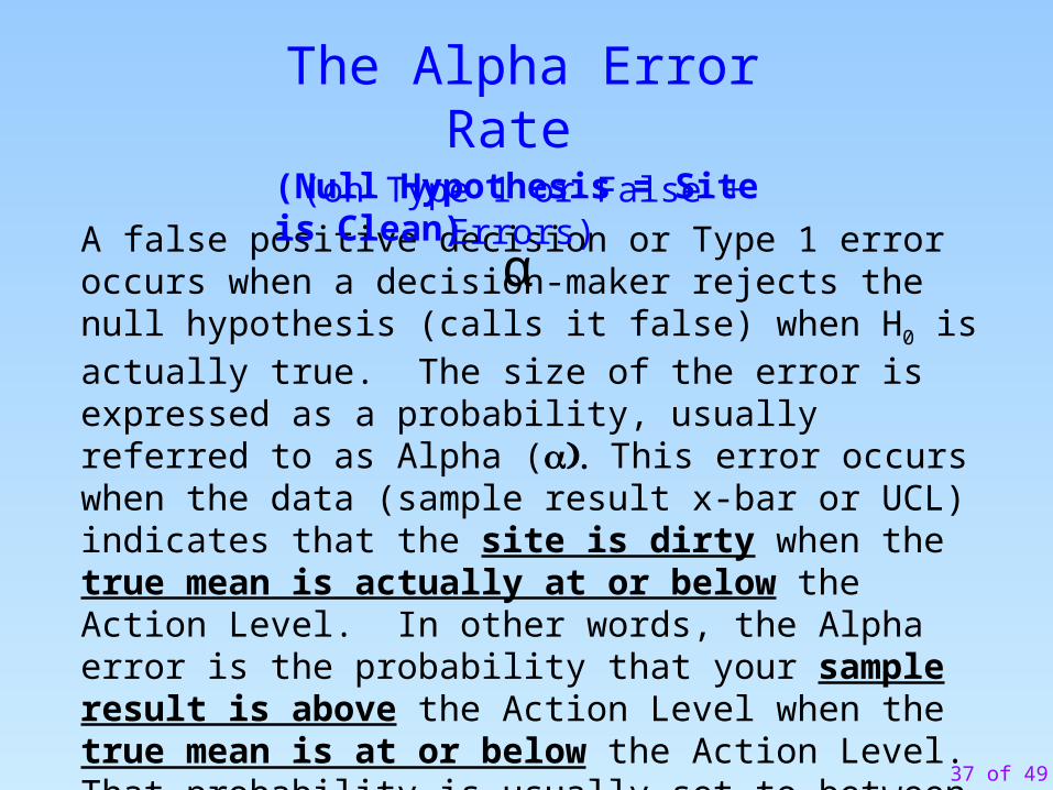
A false positive decision or Type 1 error occurs when a decision-maker rejects the null hypothesis (calls it false) when H0 is actually true. The size of the error is expressed as a probability, usually referred to as Alpha ( This error occurs when the data (sample result x-bar or UCL) indicates that the site is dirty when the true mean is actually at or below the Action Level. In other words, the Alpha error is the probability that your sample result is above the Action Level when the true mean is at or below the Action Level. That probability is usually set to between 5-1%.
(Null Hypothesis = Site is Clean)
The Alpha Error Rate (on Type 1 or False + Errors)
α

38 of 49
The Beta Error Rate (on Type 2 or False - errors)
The chance of deciding a clean site is dirty when the true mean is equal to the lower
bound of the gray region (LBGR)
Null Hypothesis = Site is Dirty

39 of 49
A false negative decision or Type 2 error occurs when a decision-maker accepts the null hypothesis (calls it true) when H0 is actually false. The size of the error is expressed as a probability, usually referred to as Beta (β This error occurs when the data (sample result x-bar or UCL) indicates that the site is dirty when the true mean is actually below the Action Level. In other words, the Beta error is the probability that your sample result is at or above the Action Level when the true mean is actually below the Action Level. That probability is negotiated and set to between 1-50%.
(Null Hypothesis = Site is Dirty)
The Beta Error Rate (on Type 2 or False – Errors)
β

40 of 49
A false negative decision or Type 2 error occurs when a decision-maker accepts the null hypothesis (calls it true) when H0 is actually false. The size of the error is expressed as a probability, usually referred to as Beta (β This error occurs when the data (sample result x-bar or UCL) indicates that the site is clean when the true mean is actually above the Action Level. In other words, the Beta error is the probability that your sample result is at or below the Action Level when the true mean is actually above the Action Level. That probability is negotiated and set to between 1-20%.
(Null Hypothesis = Site is Clean)
The Beta Error Rate (on Type 2 or False – Errors)
β

41 of 49
Evaluate Alpha & Beta Errors
True Mean Concentration
0 ∞100
Action Level
75
LBGR
µ:α
AlphaError
BetaError
µ:β
42 of 49
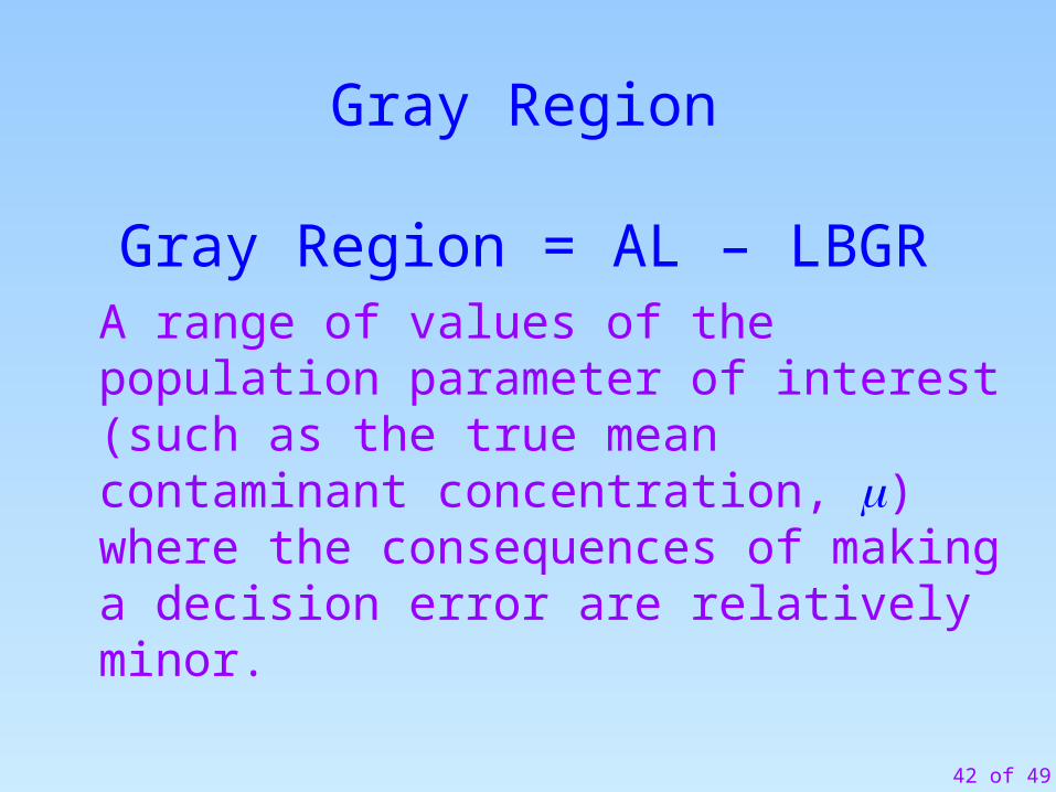
A range of values of the population parameter of interest (such as the true mean contaminant concentration, ) where the consequences of making a decision error are relatively minor.
Gray Region
Gray Region = AL – LBGR

43 of 49
The Gray Region is bounded on one side by the action level, and on the other side by the parametervalue where the consequences of decision error beginsto be significant. This point is labeled LBGR, whichstands for Lower Bound of the Gray Region.
Gray Region & LBGR
Gray Region = AL – LBGR

44 of 49
=AL – Width of GR = AL – LBGR
The Lower Bound of the Gray Region () is defined as the hypothetical true mean
concentration where the site should be declared clean with a reasonably high probability.
(Null Hypothesis = Site is Dirty)
The Width of Gray Region

45 of 49
= – AL Width of GR = UBGR – AL
The Upper Bound of the Gray Region ()
is defined as the hypothetical true mean concentration where the site should be declared
dirty with a reasonably high probability.
(Null Hypothesis = Site is Clean)
The Width of Gray Region

46 of 49
Coefficient of Variation:
CV = s / x-barIf CV > 1, not Normal
Relative Standard Deviation:
RSD (%) = CV * 100If RSD > 100%, not Normal

47 of 49
SHOW VST Filefor
Coefficient of Variationand
RSD

48 of 49
Decisions about population parameters, such as the true mean, , and the true standard deviation, , are based on statistics such as the sample mean, , and the sample standard deviation, s. Since these decisions are based on incomplete information, they will be in error.
Summary
X
49 of 49
End of Module 3
Thank you
Questions?
We will now take a 75 minute lunch break.
Please be back in 1 hour and 15 minutes.