Embed Size (px)
Citation preview

1
Overview of Query Evaluation
Chapter 12
2
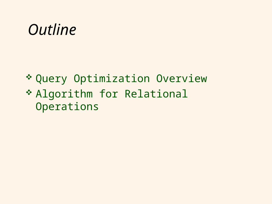
Outline
Query Optimization Overview Algorithm for Relational Operations
3
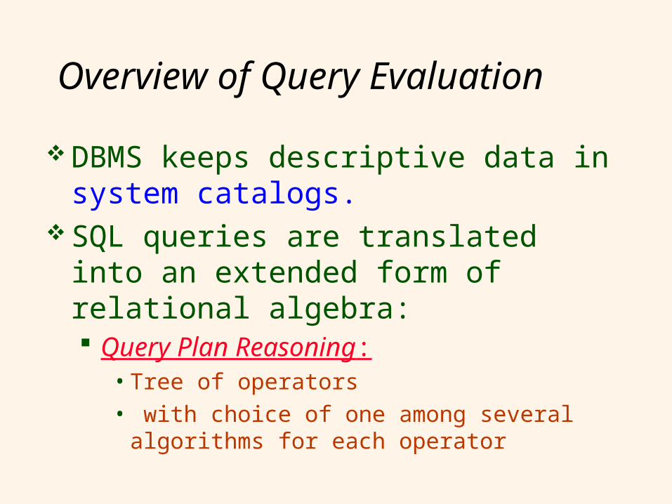
Overview of Query Evaluation
DBMS keeps descriptive data in system catalogs.
SQL queries are translated into an extended form of relational algebra: Query Plan Reasoning:
• Tree of operators• with choice of one among several
algorithms for each operator

Query Plan Evaluation
Reserves Sailors
sid=sid
bid=100 rating > 5
sname Query Plan Execution:
•Each operator typically implemented using a `pull’ interface
•when an operator is `pulled’ for next output tuples, it `pulls’ on its inputs and computes them.
5
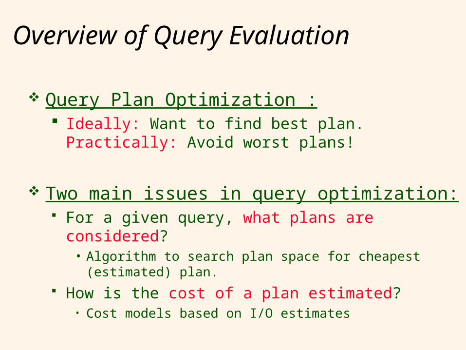
Overview of Query Evaluation
Query Plan Optimization : Ideally: Want to find best plan.
Practically: Avoid worst plans!
Two main issues in query optimization: For a given query, what plans are considered?
• Algorithm to search plan space for cheapest (estimated) plan.
How is the cost of a plan estimated?• Cost models based on I/O estimates
9
Query Processing
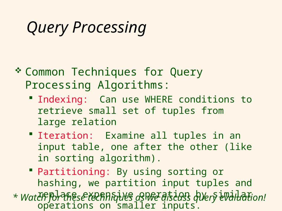
Common Techniques for Query Processing Algorithms: Indexing: Can use WHERE conditions to
retrieve small set of tuples from large relation Iteration: Examine all tuples in an input
table, one after the other (like in sorting algorithm).
Partitioning: By using sorting or hashing, we partition input tuples and replace expensive operation by similar operations on smaller inputs.* Watch for these techniques as we discuss query evaluation!
10
Access Paths
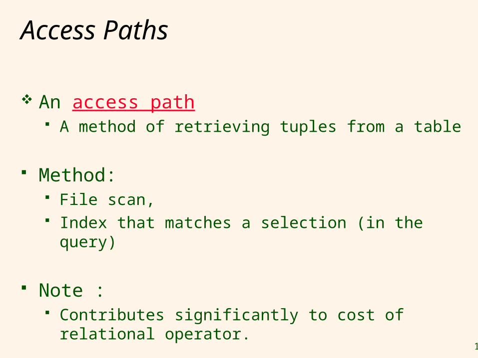
An access path A method of retrieving tuples from a table
Method: File scan, Index that matches a selection (in the query)
Note : Contributes significantly to cost of relational
operator.
11
Matching an Access Path
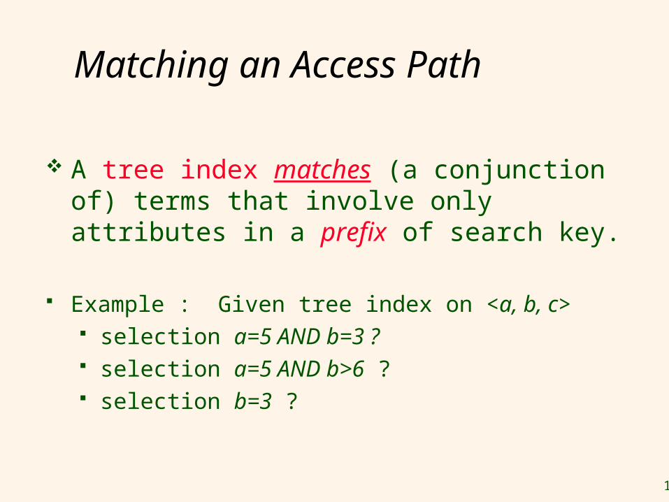
A tree index matches (a conjunction of) terms that involve only attributes in a prefix of search key.
Example : Given tree index on <a, b, c> selection a=5 AND b=3 ? selection a=5 AND b>6 ? selection b=3 ?
12
Matching an Access Path
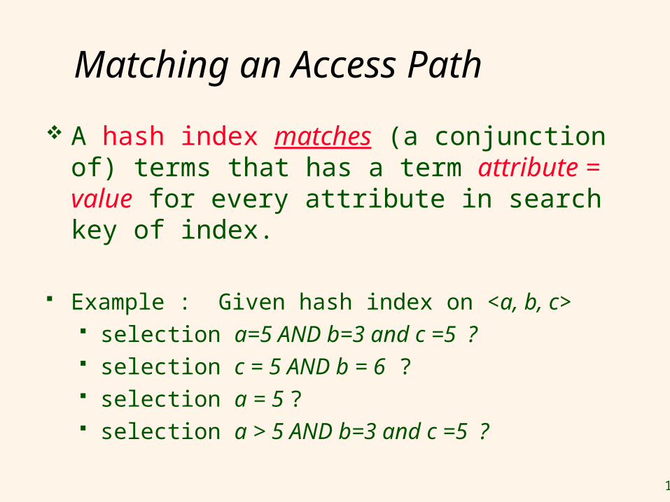
A hash index matches (a conjunction of) terms that has a term attribute = value for every attribute in search key of index.
Example : Given hash index on <a, b, c> selection a=5 AND b=3 and c =5 ? selection c = 5 AND b = 6 ? selection a = 5 ? selection a > 5 AND b=3 and c =5 ?

14
Query Evaluation of Selection
15
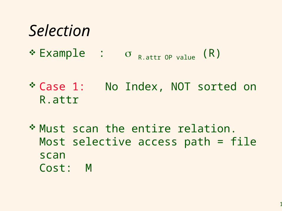
Selection Example : R.attr OP value (R)
Case 1: No Index, NOT sorted on R.attr
Must scan the entire relation.Most selective access path = file scanCost: M
16
Selection
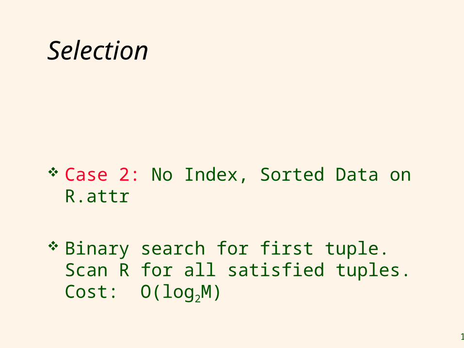
Case 2: No Index, Sorted Data on R.attr
Binary search for first tuple.Scan R for all satisfied tuples.Cost: O(log2M)
17
Selection Using B+ tree index
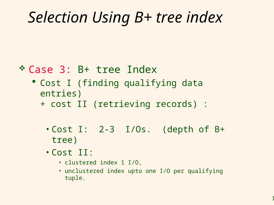
Case 3: B+ tree Index Cost I (finding qualifying data entries)
+ cost II (retrieving records) :
• Cost I: 2-3 I/Os. (depth of B+ tree)• Cost II:
• clustered index 1 I/O, • unclustered index upto one I/O per qualifying tuple.
18
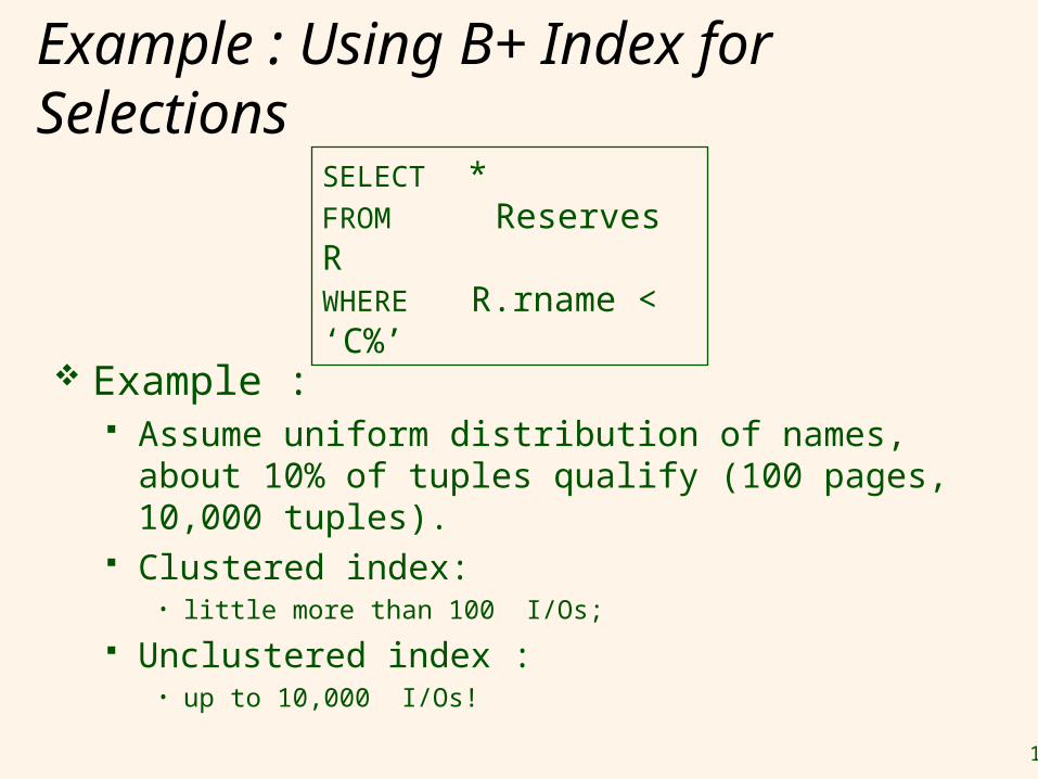
Example : Using B+ Index for Selections
Example : Assume uniform distribution of names, about
10% of tuples qualify (100 pages, 10,000 tuples).
Clustered index: • little more than 100 I/Os;
Unclustered index :• up to 10,000 I/Os!
SELECT *FROM Reserves RWHERE R.rname < ‘C%’
19
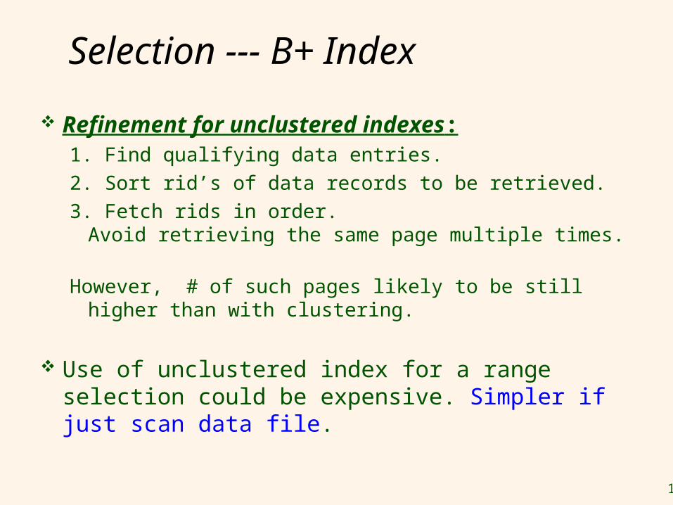
Selection --- B+ Index
Refinement for unclustered indexes: 1. Find qualifying data entries.2. Sort rid’s of data records to be retrieved.3. Fetch rids in order.
Avoid retrieving the same page multiple times.
However, # of such pages likely to be still higher than with clustering.
Use of unclustered index for a range selection could be expensive. Simpler if just scan data file.
20
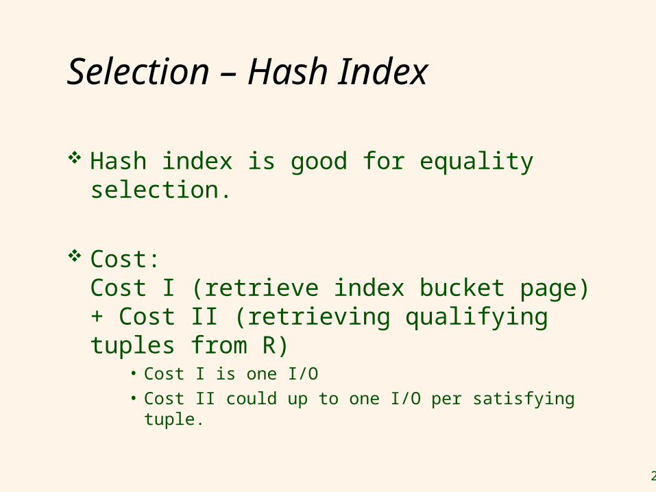
Selection – Hash Index
Hash index is good for equality selection.
Cost: Cost I (retrieve index bucket page) + Cost II (retrieving qualifying tuples from R)
• Cost I is one I/O• Cost II could up to one I/O per satisfying tuple.
21
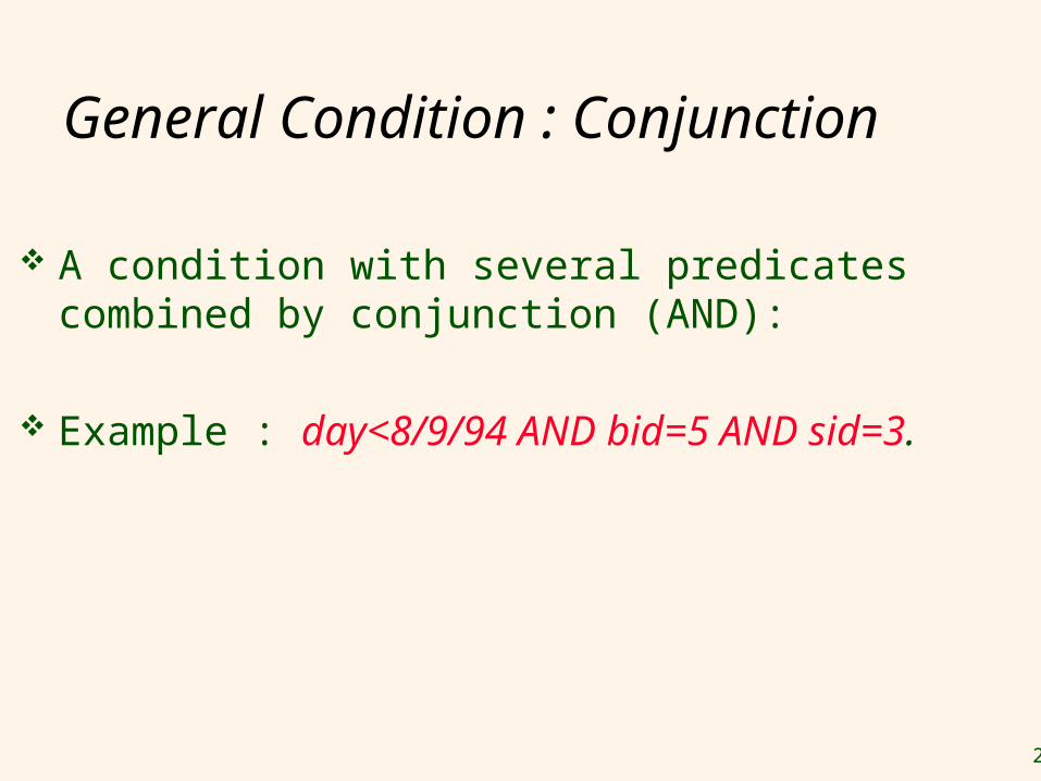
General Condition : Conjunction
A condition with several predicates combined by conjunction (AND):
Example : day<8/9/94 AND bid=5 AND sid=3.
22
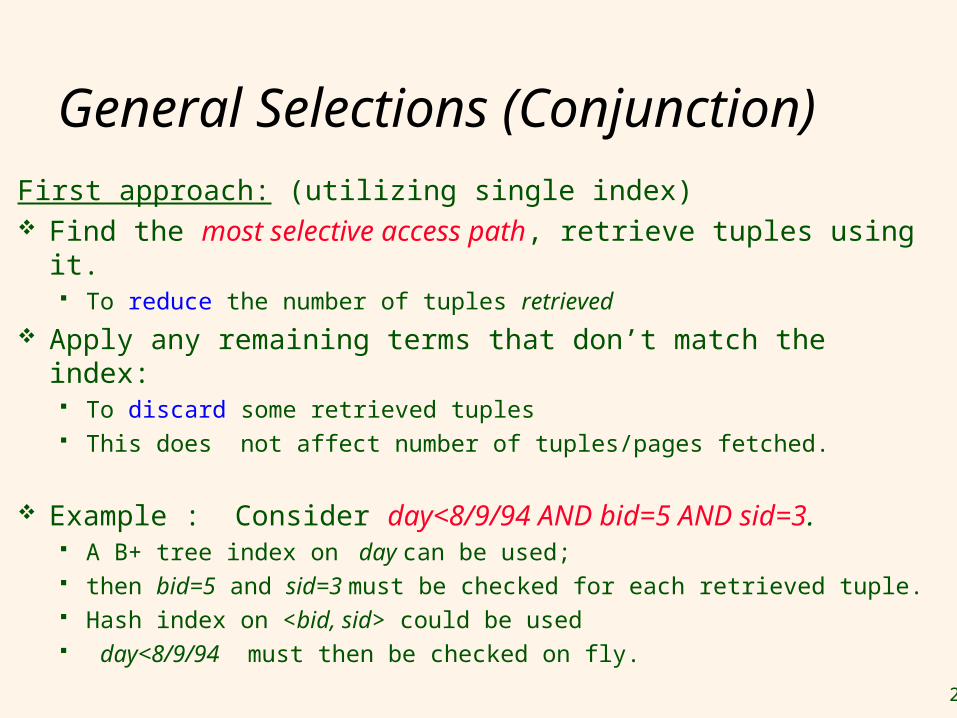
General Selections (Conjunction)
First approach: (utilizing single index) Find the most selective access path, retrieve tuples
using it. To reduce the number of tuples retrieved
Apply any remaining terms that don’t match the index: To discard some retrieved tuples This does not affect number of tuples/pages fetched.
Example : Consider day<8/9/94 AND bid=5 AND sid=3. A B+ tree index on day can be used; then bid=5 and sid=3 must be checked for each retrieved tuple. Hash index on <bid, sid> could be used day<8/9/94 must then be checked on fly.
23
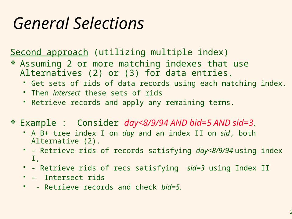
General Selections
Second approach (utilizing multiple index) Assuming 2 or more matching indexes that use
Alternatives (2) or (3) for data entries. Get sets of rids of data records using each matching index. Then intersect these sets of rids Retrieve records and apply any remaining terms.
Example : Consider day<8/9/94 AND bid=5 AND sid=3. A B+ tree index I on day and an index II on sid, both Alternative
(2). - Retrieve rids of records satisfying day<8/9/94 using index I, - Retrieve rids of recs satisfying sid=3 using Index II - Intersect rids - Retrieve records and check bid=5.
24
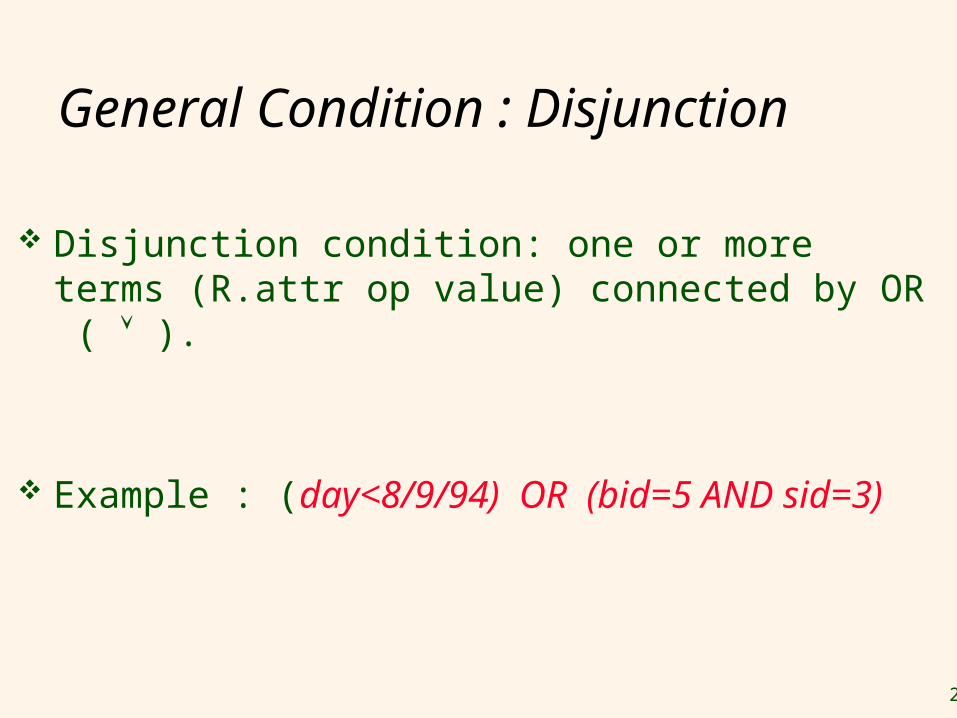
General Condition : Disjunction
Disjunction condition: one or more terms (R.attr op value) connected by OR ( ).
Example : (day<8/9/94) OR (bid=5 AND sid=3)
25
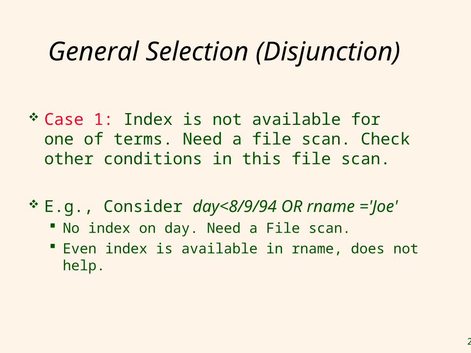
General Selection (Disjunction)
Case 1: Index is not available for one of terms. Need a file scan. Check other conditions in this file scan.
E.g., Consider day<8/9/94 OR rname ='Joe' No index on day. Need a File scan. Even index is available in rname, does not
help.
26
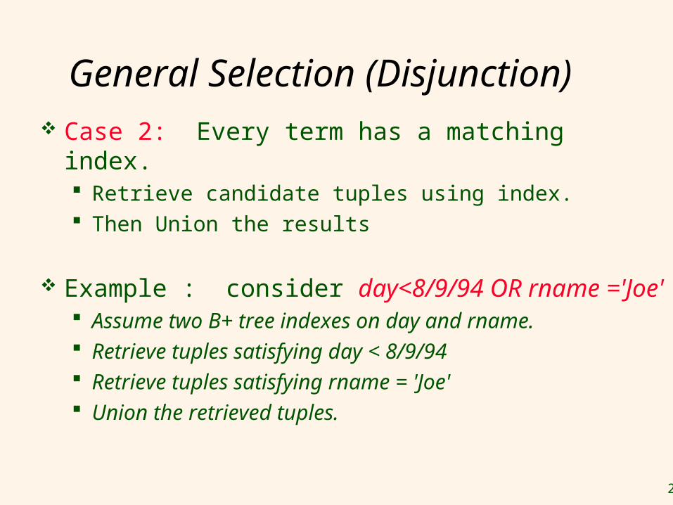
General Selection (Disjunction)
Case 2: Every term has a matching index. Retrieve candidate tuples using index. Then Union the results
Example : consider day<8/9/94 OR rname ='Joe' Assume two B+ tree indexes on day and rname. Retrieve tuples satisfying day < 8/9/94 Retrieve tuples satisfying rname = 'Joe' Union the retrieved tuples.

27
Query Evaluation of Projection
28
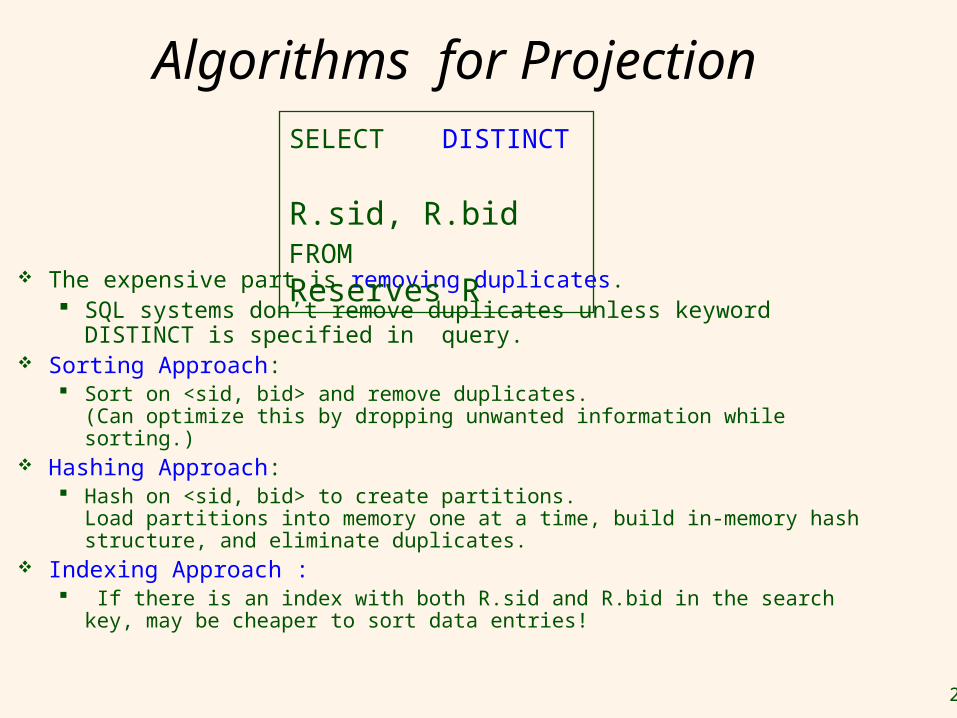
Algorithms for Projection
The expensive part is removing duplicates. SQL systems don’t remove duplicates unless keyword DISTINCT
is specified in query. Sorting Approach:
Sort on <sid, bid> and remove duplicates. (Can optimize this by dropping unwanted information while sorting.)
Hashing Approach: Hash on <sid, bid> to create partitions.
Load partitions into memory one at a time, build in-memory hash structure, and eliminate duplicates.
Indexing Approach : If there is an index with both R.sid and R.bid in the search key, may be
cheaper to sort data entries!
SELECT DISTINCT R.sid, R.bidFROM Reserves R

29
Query Evaluation of Joins
30
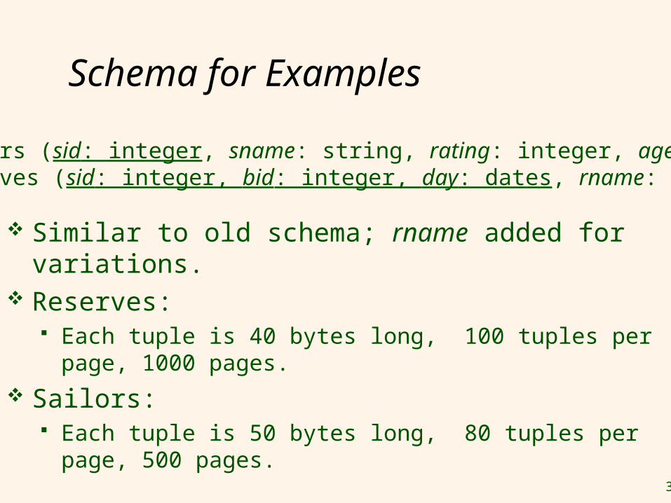
Schema for Examples
Similar to old schema; rname added for variations.
Reserves: Each tuple is 40 bytes long, 100 tuples per page,
1000 pages. Sailors:
Each tuple is 50 bytes long, 80 tuples per page, 500 pages.
Sailors (sid: integer, sname: string, rating: integer, age: real)Reserves (sid: integer, bid: integer, day: dates, rname: string)
31
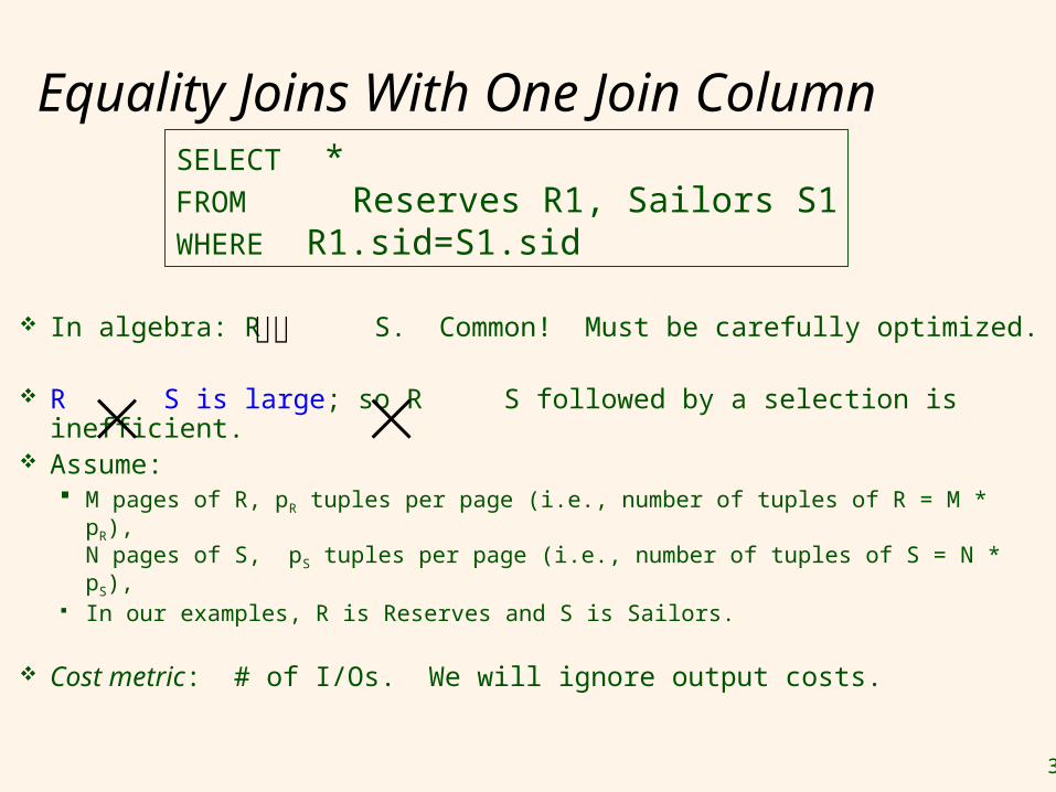
Equality Joins With One Join Column
In algebra: R S. Common! Must be carefully optimized.
R S is large; so R S followed by a selection is inefficient. Assume:
M pages of R, pR tuples per page (i.e., number of tuples of R = M * pR), N pages of S, pS tuples per page (i.e., number of tuples of S = N * pS),
In our examples, R is Reserves and S is Sailors.
Cost metric: # of I/Os. We will ignore output costs.
SELECT *FROM Reserves R1, Sailors S1WHERE R1.sid=S1.sid
32
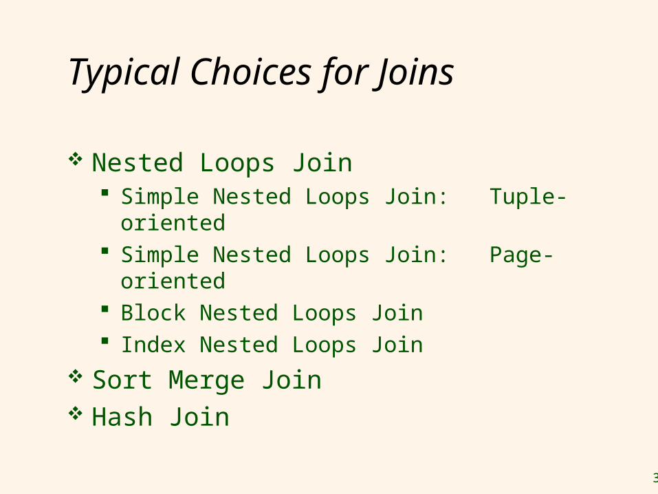
Typical Choices for Joins
Nested Loops Join Simple Nested Loops Join: Tuple-oriented Simple Nested Loops Join: Page-oriented Block Nested Loops Join Index Nested Loops Join
Sort Merge Join Hash Join
33
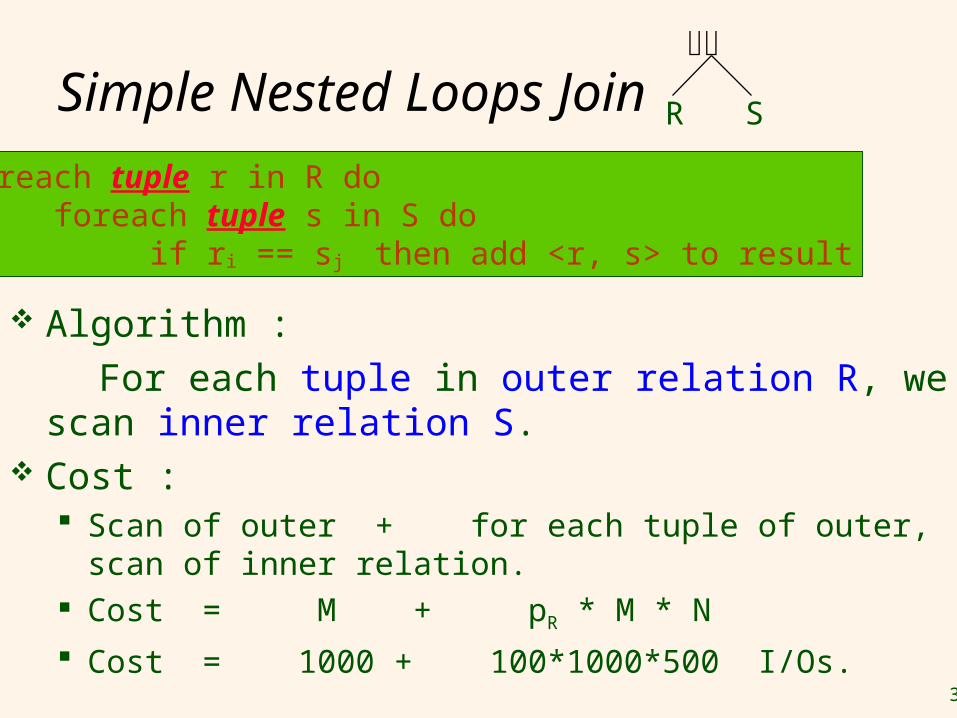
Simple Nested Loops Join
Algorithm : For each tuple in outer relation R, we scan
inner relation S. Cost :
Scan of outer + for each tuple of outer, scan of inner relation.
Cost = M + pR * M * N Cost = 1000 + 100*1000*500 I/Os.
foreach tuple r in R doforeach tuple s in S do
if ri == sj then add <r, s> to result
R S
34
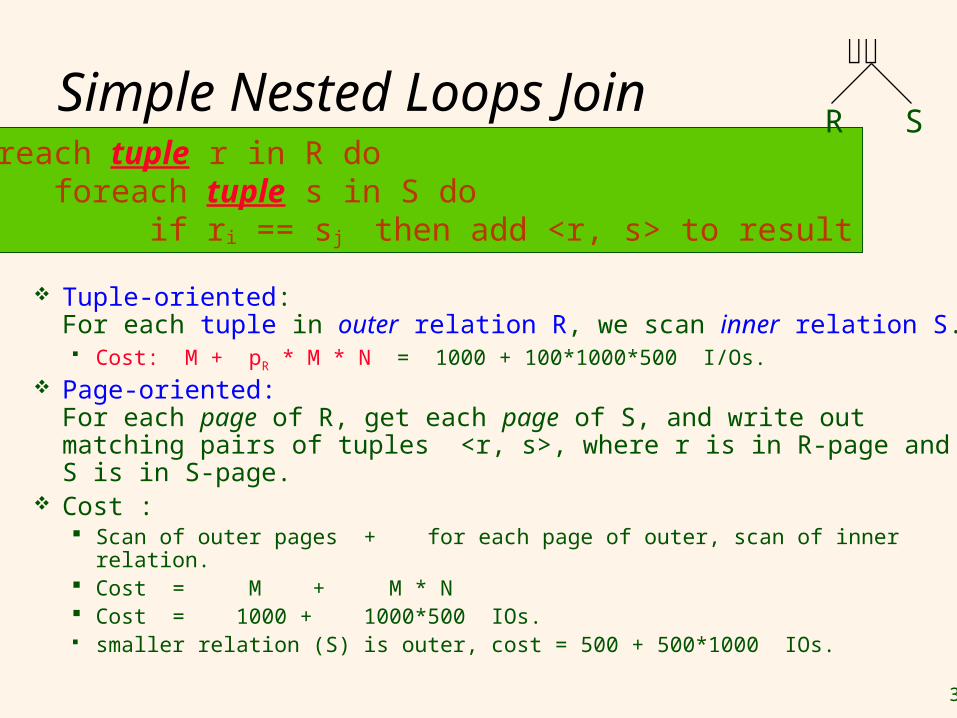
Simple Nested Loops Join
Tuple-oriented: For each tuple in outer relation R, we scan inner relation S. Cost: M + pR * M * N = 1000 + 100*1000*500 I/Os.
Page-oriented: For each page of R, get each page of S, and write out matching pairs of tuples <r, s>, where r is in R-page and S is in S-page.
Cost : Scan of outer pages + for each page of outer, scan of inner relation. Cost = M + M * N Cost = 1000 + 1000*500 IOs. smaller relation (S) is outer, cost = 500 + 500*1000 IOs.
foreach tuple r in R doforeach tuple s in S do
if ri == sj then add <r, s> to result
R S
35
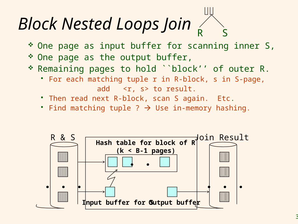
Block Nested Loops Join One page as input buffer for scanning inner S, One page as the output buffer, Remaining pages to hold ``block’’ of outer R.
For each matching tuple r in R-block, s in S-page, add <r, s> to result. Then read next R-block, scan S again. Etc. Find matching tuple ? Use in-memory hashing.
. . .
. . .
R & SHash table for block of R
(k < B-1 pages)
Input buffer for S Output buffer
. . .
Join Result
R S
36
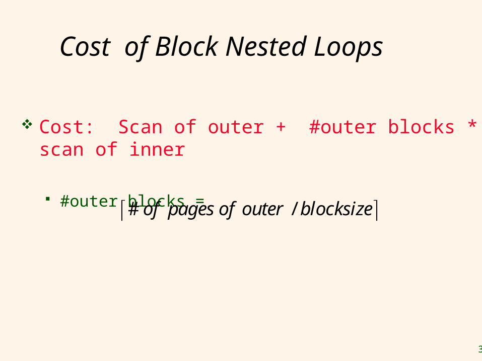
Cost of Block Nested Loops
Cost: Scan of outer + #outer blocks * scan of inner
#outer blocks = # /of pages of outer blocksize
37
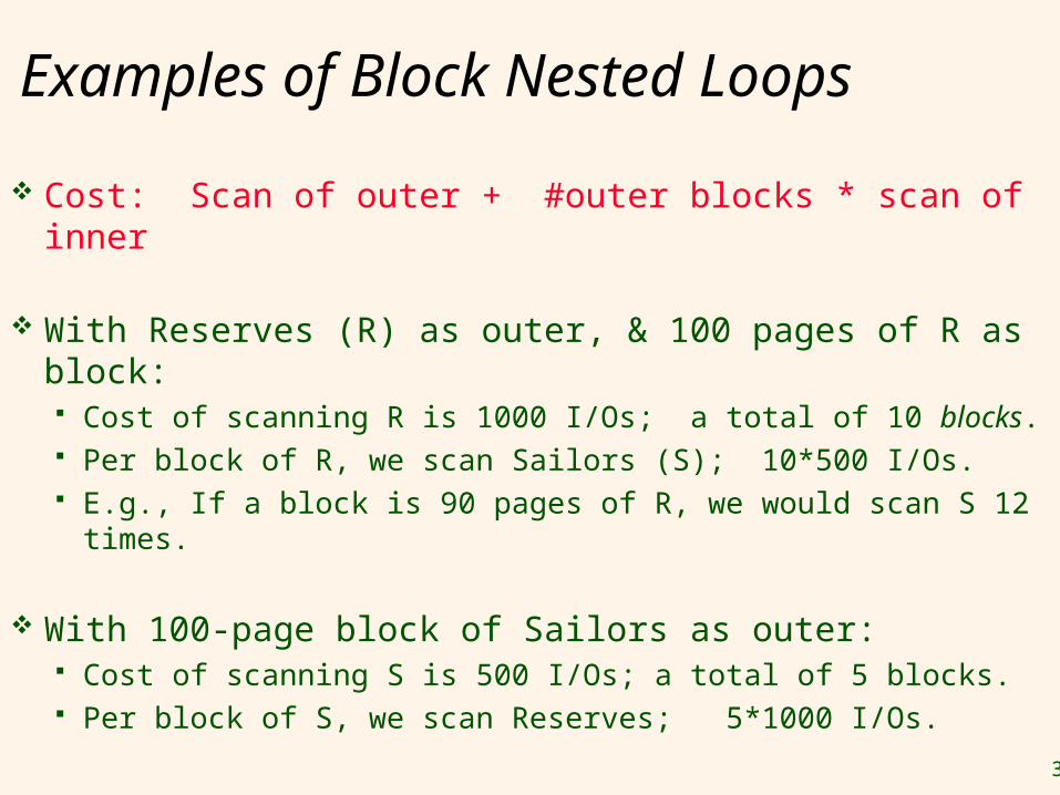
Examples of Block Nested Loops Cost: Scan of outer + #outer blocks * scan of inner
With Reserves (R) as outer, & 100 pages of R as block: Cost of scanning R is 1000 I/Os; a total of 10 blocks. Per block of R, we scan Sailors (S); 10*500 I/Os. E.g., If a block is 90 pages of R, we would scan S 12 times.
With 100-page block of Sailors as outer: Cost of scanning S is 500 I/Os; a total of 5 blocks. Per block of S, we scan Reserves; 5*1000 I/Os.
38
Examples of Block Nested Loops
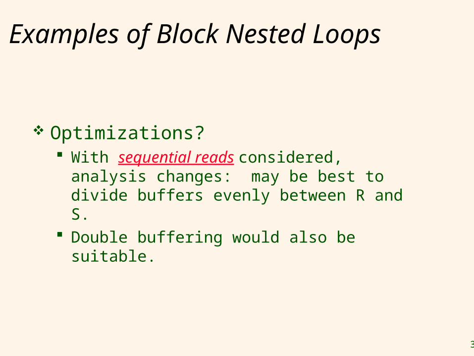
Optimizations? With sequential reads considered,
analysis changes: may be best to divide buffers evenly between R and S.
Double buffering would also be suitable.
40
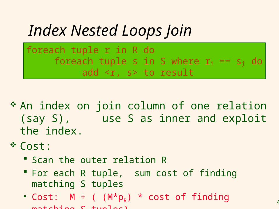
Index Nested Loops Join
An index on join column of one relation (say S), use S as inner and exploit the index.
Cost: Scan the outer relation R For each R tuple, sum cost of finding matching S
tuples Cost: M + ( (M*pR) * cost of finding matching S
tuples)
foreach tuple r in R doforeach tuple s in S where ri == sj do
add <r, s> to result
41
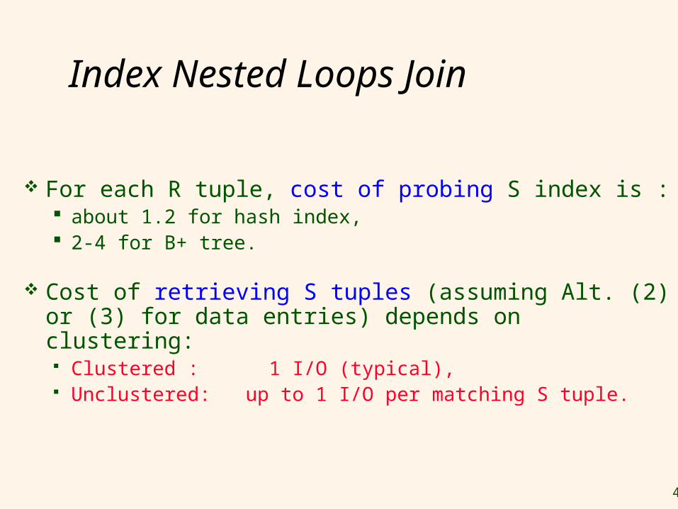
Index Nested Loops Join
For each R tuple, cost of probing S index is : about 1.2 for hash index, 2-4 for B+ tree.
Cost of retrieving S tuples (assuming Alt. (2) or (3) for data entries) depends on clustering: Clustered : 1 I/O (typical), Unclustered: up to 1 I/O per matching S tuple.
43
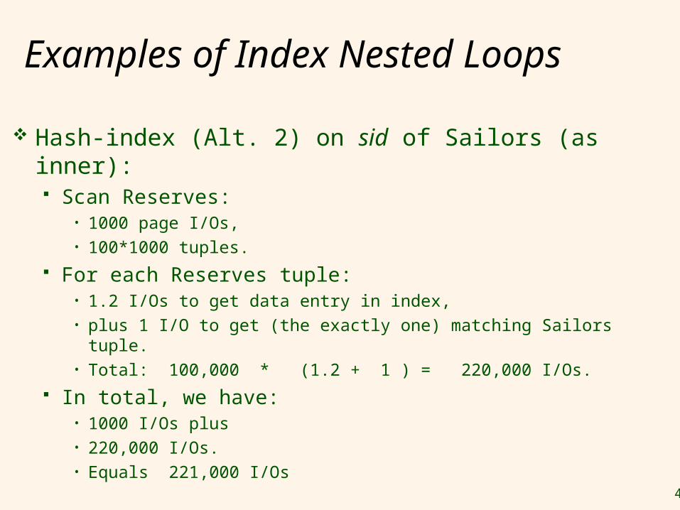
Examples of Index Nested Loops
Hash-index (Alt. 2) on sid of Sailors (as inner): Scan Reserves:
• 1000 page I/Os, • 100*1000 tuples.
For each Reserves tuple: • 1.2 I/Os to get data entry in index, • plus 1 I/O to get (the exactly one) matching Sailors tuple. • Total: 100,000 * (1.2 + 1 ) = 220,000 I/Os.
In total, we have:• 1000 I/Os plus • 220,000 I/Os.• Equals 221,000 I/Os
44
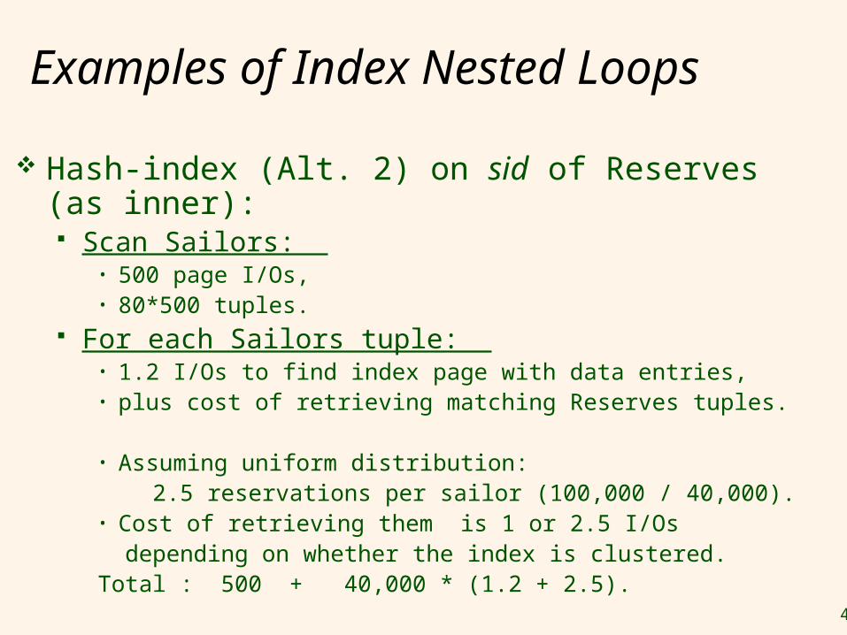
Examples of Index Nested Loops
Hash-index (Alt. 2) on sid of Reserves (as inner): Scan Sailors:
• 500 page I/Os, • 80*500 tuples.
For each Sailors tuple: • 1.2 I/Os to find index page with data entries, • plus cost of retrieving matching Reserves tuples.
• Assuming uniform distribution: 2.5 reservations per sailor (100,000 / 40,000). • Cost of retrieving them is 1 or 2.5 I/Os depending on whether the index is clustered.Total : 500 + 40,000 * (1.2 + 2.5).

46
Simple vs. Index Nested Loops Join Assume: M Pages in R, pR tuples per page,
N Pages in S, pS tuples per page,B Buffer Pages.
Nested Loops Join Simple Nested Loops Join
• Tuple-oriented: M + pR * M * N• Page-oriented: M + M * N• Smaller as outer helps.
Block Nested Loops Join• M + N*M/(B-2) • Dividing buffer evenly between R and S helps.
Index Nested Loops Join• M + ( (M*pR) * cost of finding matching S tuples) • cost of finding matching S tuples = cost of Probe + cost of
retrieving With unclustered index, if number of matching inner
tuples for each outer tuple is small, cost of INLJ is much smaller than SNLJ.
47
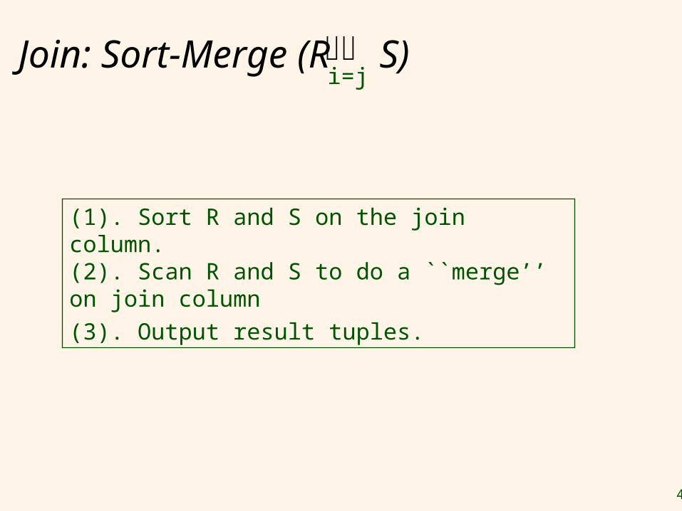
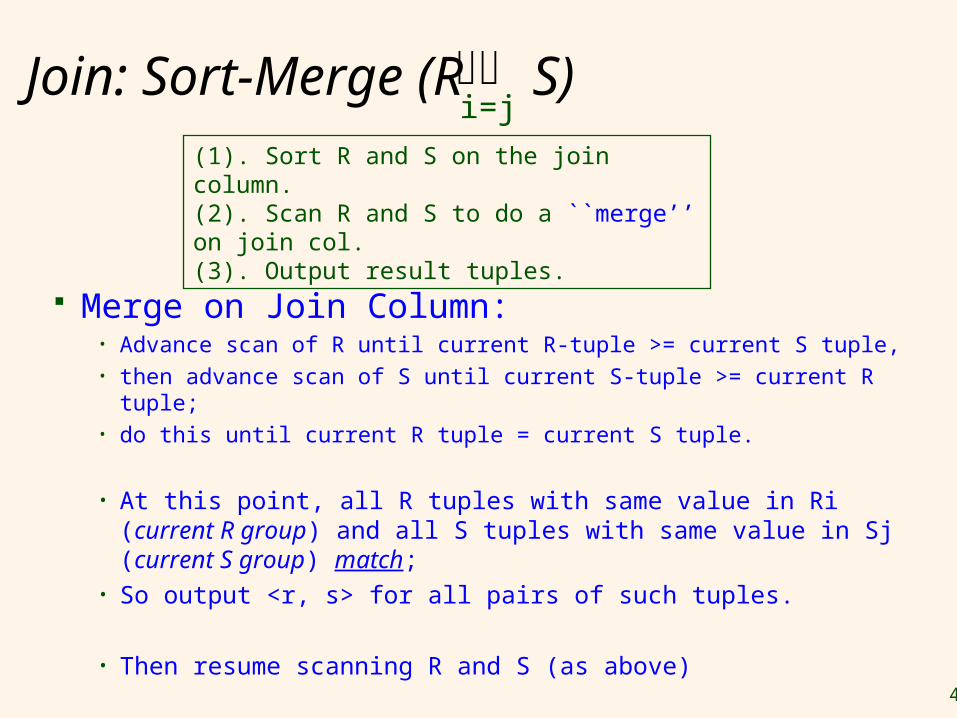
Join: Sort-Merge (R S)i=j
(1). Sort R and S on the join column.(2). Scan R and S to do a ``merge’’ on join column(3). Output result tuples.
48
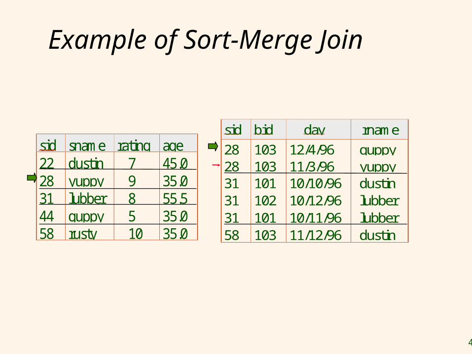
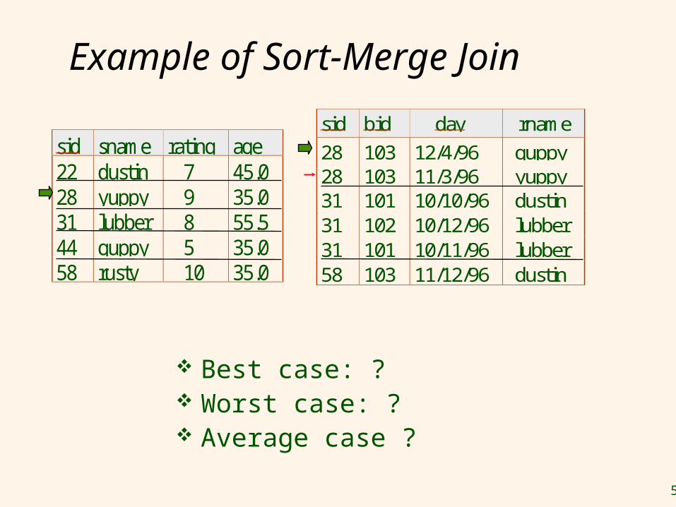
Example of Sort-Merge Join
sid sname rating age22 dustin 7 45.028 yuppy 9 35.031 lubber 8 55.544 guppy 5 35.058 rusty 10 35.0
sid bid day rname
28 103 12/4/96 guppy28 103 11/3/96 yuppy31 101 10/10/96 dustin31 102 10/12/96 lubber31 101 10/11/96 lubber58 103 11/12/96 dustin
49
Join: Sort-Merge (R S)
Merge on Join Column:• Advance scan of R until current R-tuple >= current S tuple, • then advance scan of S until current S-tuple >= current R tuple; • do this until current R tuple = current S tuple.
• At this point, all R tuples with same value in Ri (current R group) and all S tuples with same value in Sj (current S group) match;
• So output <r, s> for all pairs of such tuples.
• Then resume scanning R and S (as above)
i=j
(1). Sort R and S on the join column.(2). Scan R and S to do a ``merge’’ on join col.(3). Output result tuples.
50
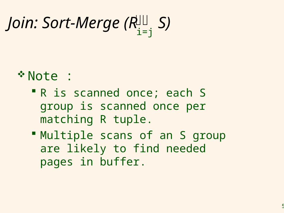
Join: Sort-Merge (R S)
Note : R is scanned once; each S group is
scanned once per matching R tuple.
Multiple scans of an S group are likely to find needed pages in buffer.
i=j
52
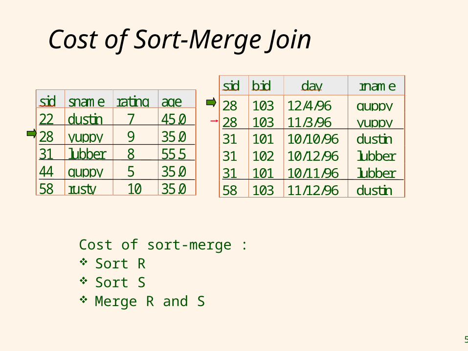
Cost of Sort-Merge Join
Cost of sort-merge : Sort R Sort S Merge R and S
sid sname rating age22 dustin 7 45.028 yuppy 9 35.031 lubber 8 55.544 guppy 5 35.058 rusty 10 35.0
sid bid day rname
28 103 12/4/96 guppy28 103 11/3/96 yuppy31 101 10/10/96 dustin31 102 10/12/96 lubber31 101 10/11/96 lubber58 103 11/12/96 dustin
53
Example of Sort-Merge Join
Best case: ? Worst case: ? Average case ?
sid sname rating age22 dustin 7 45.028 yuppy 9 35.031 lubber 8 55.544 guppy 5 35.058 rusty 10 35.0
sid bid day rname
28 103 12/4/96 guppy28 103 11/3/96 yuppy31 101 10/10/96 dustin31 102 10/12/96 lubber31 101 10/11/96 lubber58 103 11/12/96 dustin

54
Cost of Sort-Merge Join Best Case Cost: (M+N)
Already sorted. The cost of scanning, M+N
Worst Case Cost: M log M + N log N + (M+N) Many pages in R in same partition. ( Worst, all of them). The pages for this partition in S don’t fit into RAM. Re-scan S is
needed. Multiple scan S is expensive!
Note: Guarantee M+N if key-FK join, or no duplicates.
R S
55
Cost of Sort-Merge Join
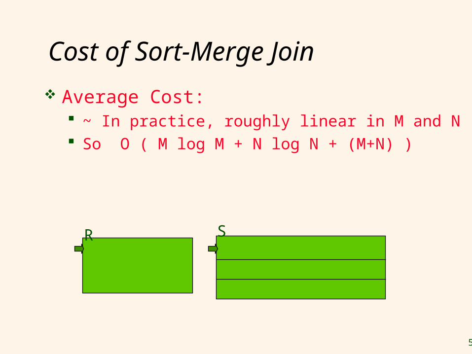
Average Cost: ~ In practice, roughly linear in M and N So O ( M log M + N log N + (M+N) )
R S

56
Comparison with Sort-Merge Join
Average Cost: O(M log M + N log N + (M+N))
Assume B = {35, 100, 300}; and R = 1000 pages, S = 500 pages
Sort-Merge Join both R and S can be sorted in 2 passes, logM = log N = 2 total join cost: 2*2*1000 + 2*2*500 +
(1000 + 500) = 7500.
Block Nested Loops Join: 2500 ~ 15000
57
Refinement of Sort-Merge Join
IDEA : Combine the merging phases when sorting R
( or S) with the merging in join algorithm.
58
Refinement of Sort-Merge Join
IDEA : Combine the merging phases when sorting R ( or S) with the merging in join algorithm. If we do the following: perform Pass 0 of sort on R;
perform Pass 0 of sort on S; merge and join on the fly – the total IO cost for join is 3 (M + N)
When is the above possible? When M/B + N/B + 1 <= B; In other words when B (B – 1) >= (M + N)(The above expression is modified from that in the book)
Cost: 3 (M + N) as follows• (read+write R and S in Pass 0) • + (read R and S in merging pass and join on fly)• + (writing of result tuples).
In example, cost goes down from 7500 to 4500 I/Os.
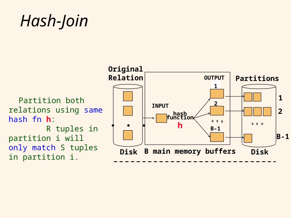
Hash-Join
Partition both relations using same hash fn h: R tuples in partition i will only match S tuples in partition i. B main memory buffers DiskDisk
Original Relation OUTPUT
2INPUT
1
hashfunction
h B-1
Partitions
1
2
B-1
. . .
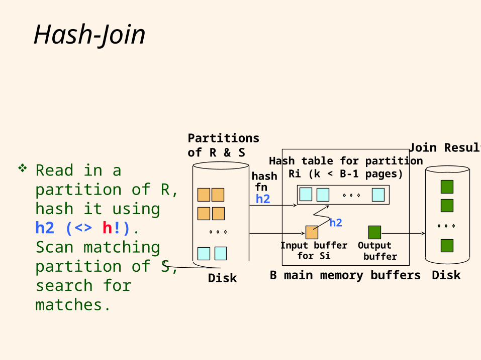
Hash-Join
Read in a partition of R, hash it using h2 (<> h!). Scan matching partition of S, search for matches.
Partitionsof R & S
Input bufferfor Si
Hash table for partitionRi (k < B-1 pages)
B main memory buffersDisk
Output buffer
Disk
Join Result
hashfnh2
h2
62
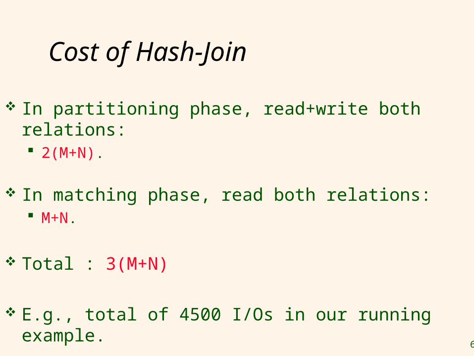
Cost of Hash-Join
In partitioning phase, read+write both relations: 2(M+N).
In matching phase, read both relations: M+N.
Total : 3(M+N)
E.g., total of 4500 I/Os in our running example.
63
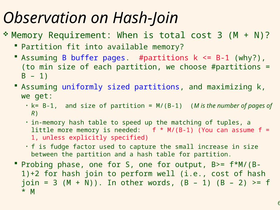
Observation on Hash-Join Memory Requirement: When is total cost 3 (M + N)?
Partition fit into available memory? Assuming B buffer pages. #partitions k <= B-1 (why?),
(to min size of each partition, we choose #partitions = B – 1)
Assuming uniformly sized partitions, and maximizing k, we get:
• k= B-1, and size of partition = M/(B-1) (M is the number of pages of R)
• in-memory hash table to speed up the matching of tuples, a little more memory is needed: f * M/(B-1) (You can assume f = 1, unless explicitly specified)
• f is fudge factor used to capture the small increase in size between the partition and a hash table for partition.
Probing phase, one for S, one for output, B>= f*M/(B-1)+2 for hash join to perform well (i.e., cost of hash join = 3 (M + N)). In other words, (B – 1) (B – 2) >= f * M
64
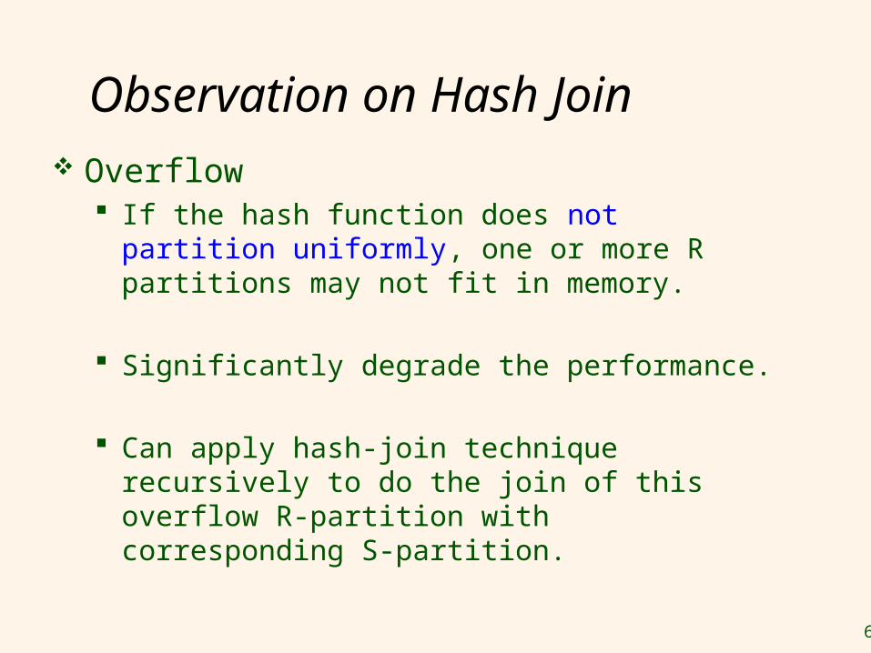
Observation on Hash Join Overflow
If the hash function does not partition uniformly, one or more R partitions may not fit in memory.
Significantly degrade the performance.
Can apply hash-join technique recursively to do the join of this overflow R-partition with corresponding S-partition.

65
Hybrid Hash-Join Idea: Do not write one of the partitions of R and
S to disk. When is it possible? We can keep one of the
partitions of the smaller relation always in memory.
B >= f * M/k (buffers for keeping a partition) + (k – 1) (keep 1 page in buffer for each of the remaining partitions)
+ 1 (1 page in buffer for reading in S (or later R)) + 1 (1 output page when reading in R)
Remember: k = number of partitions i.e., (B – (k + 1)) >= f * M/k Choose such an appropriate k (or number of partitions)
66
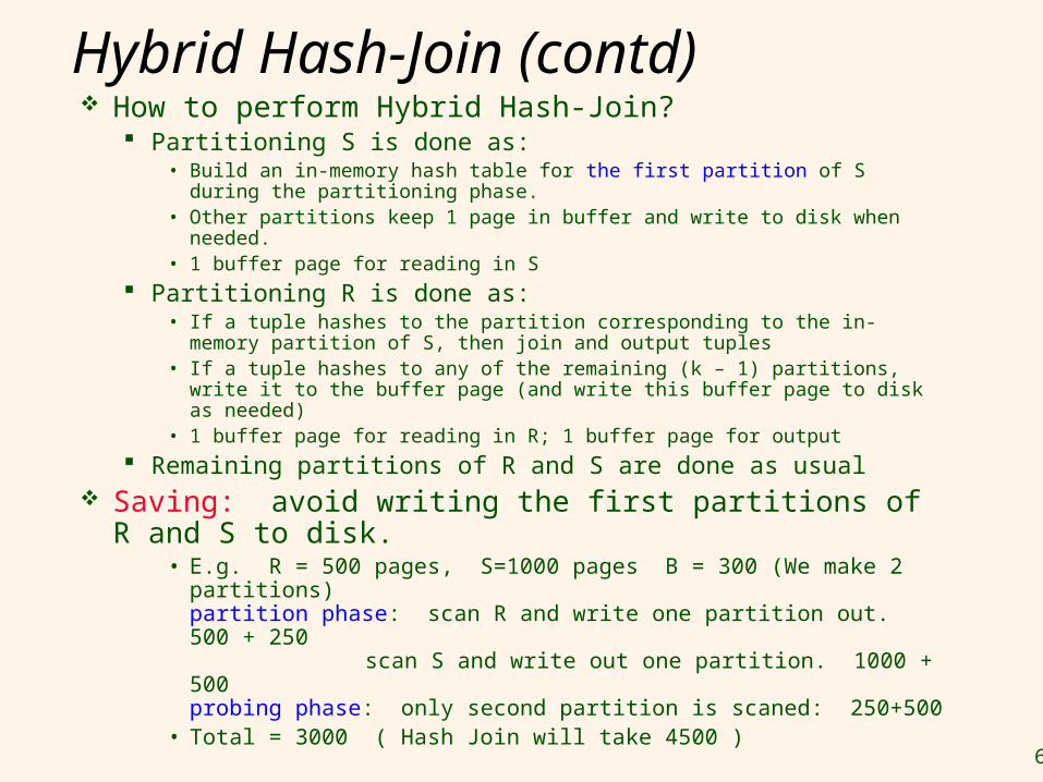
Hybrid Hash-Join (contd) How to perform Hybrid Hash-Join?
Partitioning S is done as:• Build an in-memory hash table for the first partition of S during the
partitioning phase.• Other partitions keep 1 page in buffer and write to disk when needed.• 1 buffer page for reading in S
Partitioning R is done as:• If a tuple hashes to the partition corresponding to the in-memory
partition of S, then join and output tuples• If a tuple hashes to any of the remaining (k – 1) partitions, write it to
the buffer page (and write this buffer page to disk as needed)• 1 buffer page for reading in R; 1 buffer page for output
Remaining partitions of R and S are done as usual Saving: avoid writing the first partitions of R and S
to disk. • E.g. R = 500 pages, S=1000 pages B = 300 (We make 2
partitions)partition phase: scan R and write one partition out. 500 + 250
scan S and write out one partition. 1000 + 500probing phase: only second partition is scaned: 250+500
• Total = 3000 ( Hash Join will take 4500 )
68
Hash-Join vs. Sort-Merge Join
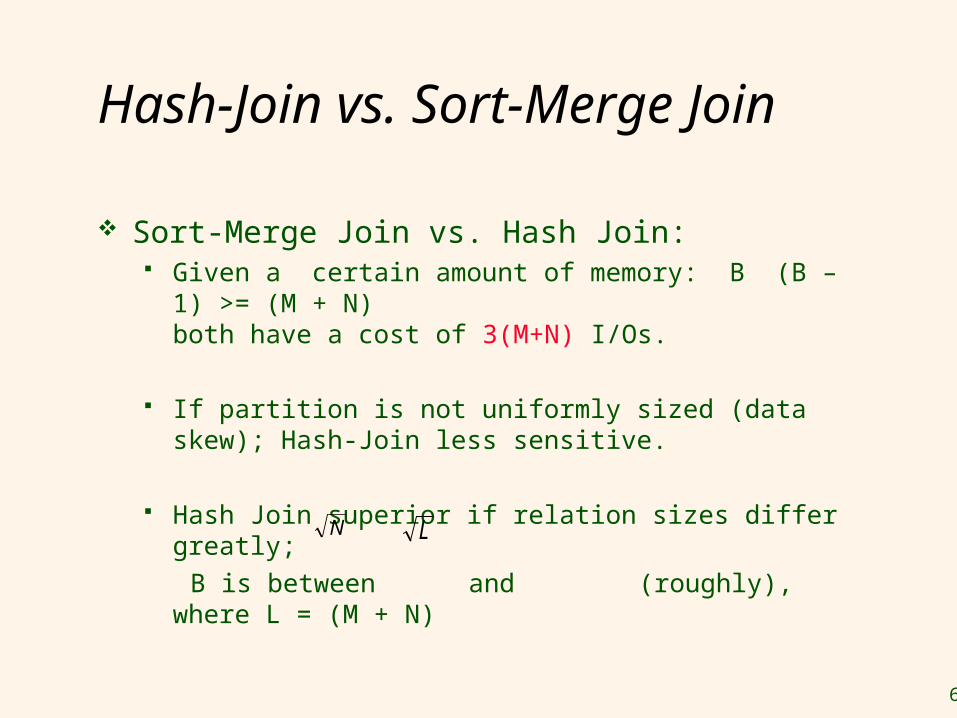
Sort-Merge Join vs. Hash Join: Given a certain amount of memory: B (B – 1) >=
(M + N) both have a cost of 3(M+N) I/Os.
If partition is not uniformly sized (data skew); Hash-Join less sensitive.
Hash Join superior if relation sizes differ greatly; B is between and (roughly), where L = (M +
N)
N L
69
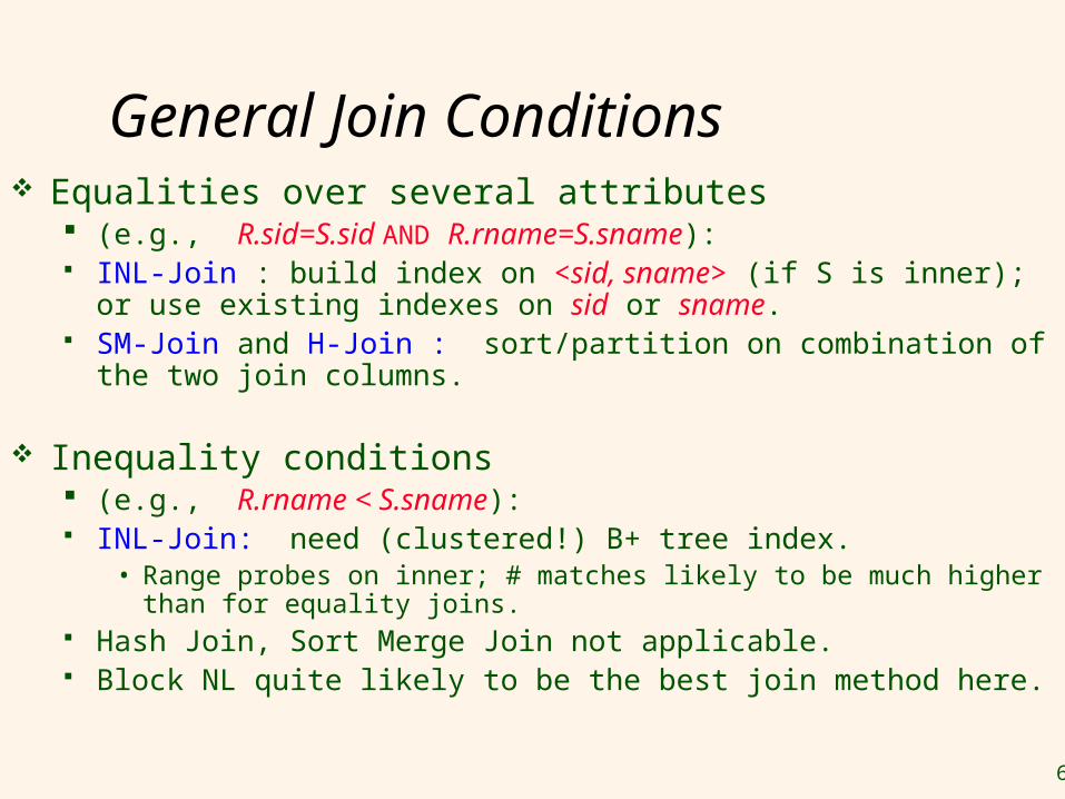
General Join Conditions Equalities over several attributes
(e.g., R.sid=S.sid AND R.rname=S.sname): INL-Join : build index on <sid, sname> (if S is inner); or use
existing indexes on sid or sname. SM-Join and H-Join : sort/partition on combination of the two
join columns.
Inequality conditions (e.g., R.rname < S.sname): INL-Join: need (clustered!) B+ tree index.
• Range probes on inner; # matches likely to be much higher than for equality joins.
Hash Join, Sort Merge Join not applicable. Block NL quite likely to be the best join method here.
70
Summary
There are several alternative evaluation algorithms for each relational operator.
71
Conclusion
Not one method wins !
Optimizer must assess situation to select best possible candidate