1 Peak-to-Average Power Ratio (PAPR) One of the main problems in OFDM system is large PAPR /PAR(increased complexity of the ADC and DAC, and reduced efficiency

1

Peak-to-Average Power Ratio (PAPR)

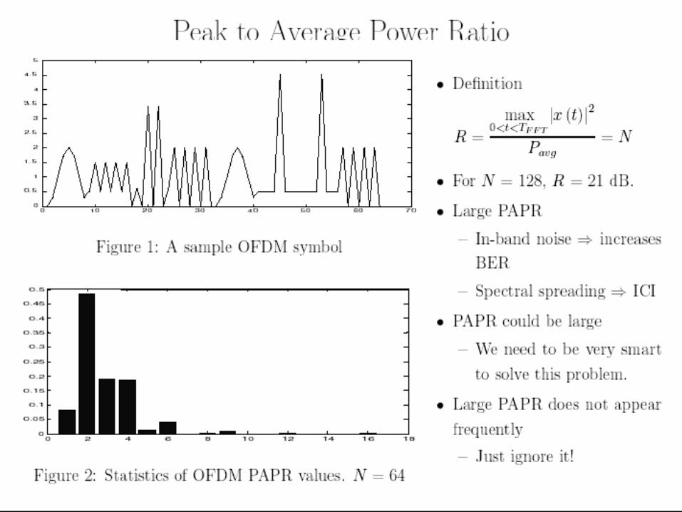
One of the main problems in OFDM system is large PAPR /PAR(increased complexity of the ADC and DAC, and reduced efficiency of RF power amplifier, and etc.)

An OFDM signal consists of a number of independently modulated subcarriers, which can give a large PAPR /PAR when added up coherently.

2

3

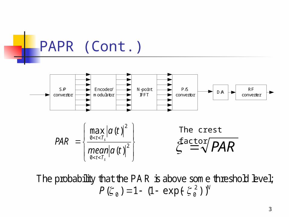
PAPR (Cont.)

S/Pconvertor

Encoder/modulator

N-pointIFFT

P/Sconvertor

D/ARF

converter

2

0

2

0

)(

)(max

tamean

taPAR

s

s

Tt

Tt

PAR

The crest factor

The probability that the PAR is above some threshold level; NP ))exp(1(1)( 2

00

4

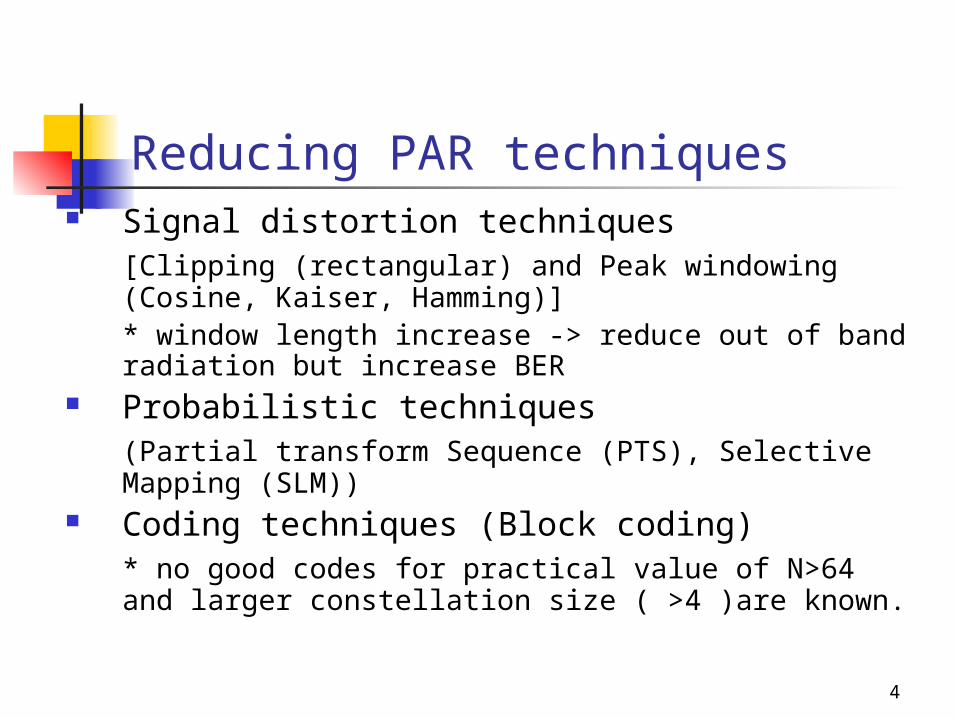
Reducing PAR techniques Signal distortion techniques

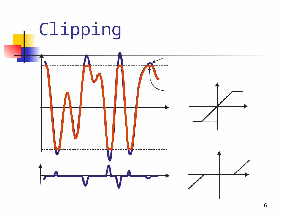
[Clipping (rectangular) and Peak windowing (Cosine, Kaiser, Hamming)]* window length increase -> reduce out of band radiation but increase BER

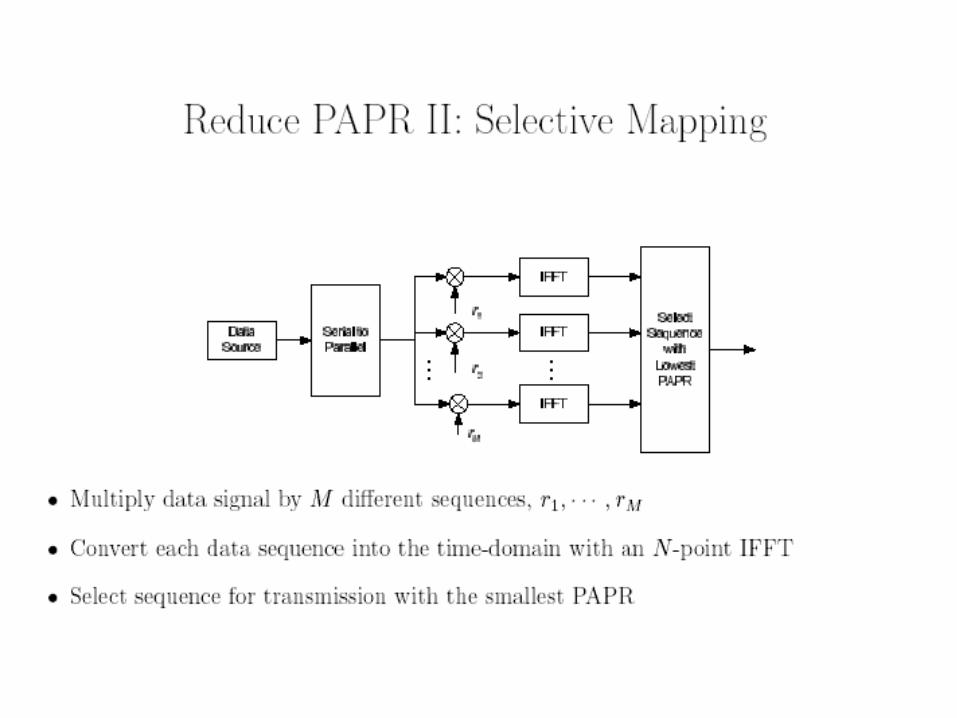
Probabilistic techniques(Partial transform Sequence (PTS), Selective Mapping (SLM))

Coding techniques (Block coding)* no good codes for practical value of N>64 and larger constellation size ( >4 )are known.

5

6

Clipping

7

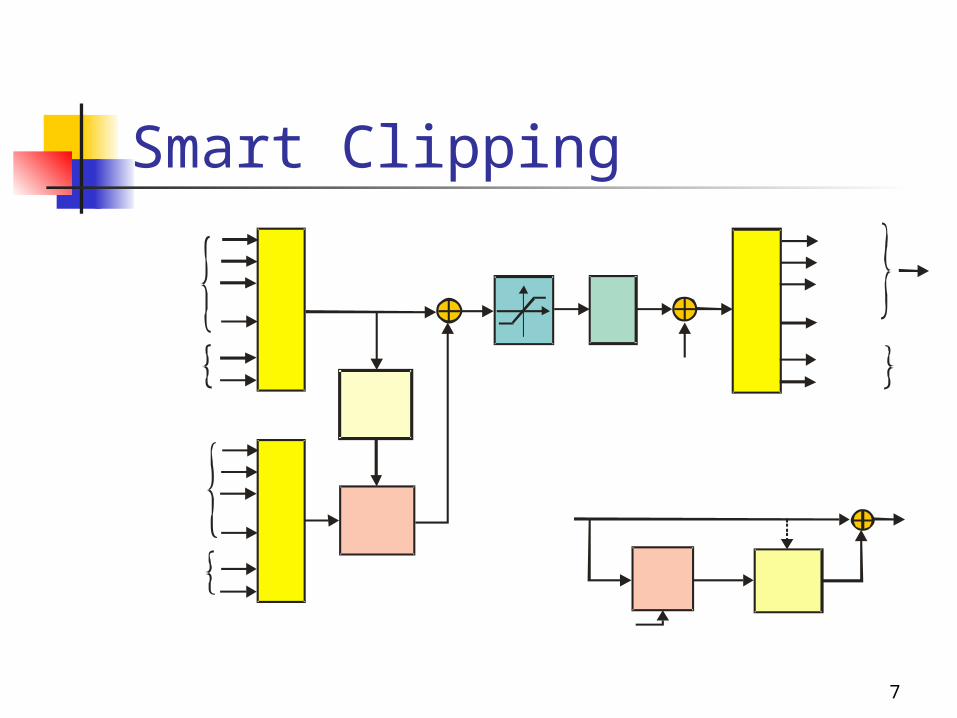
Smart Clipping

8

9

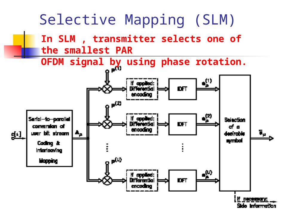
Selective Mapping (SLM)In SLM , transmitter selects one of the smallest PAROFDM signal by using phase rotation.

10

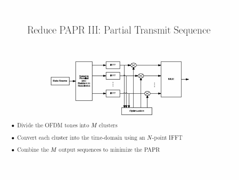
11

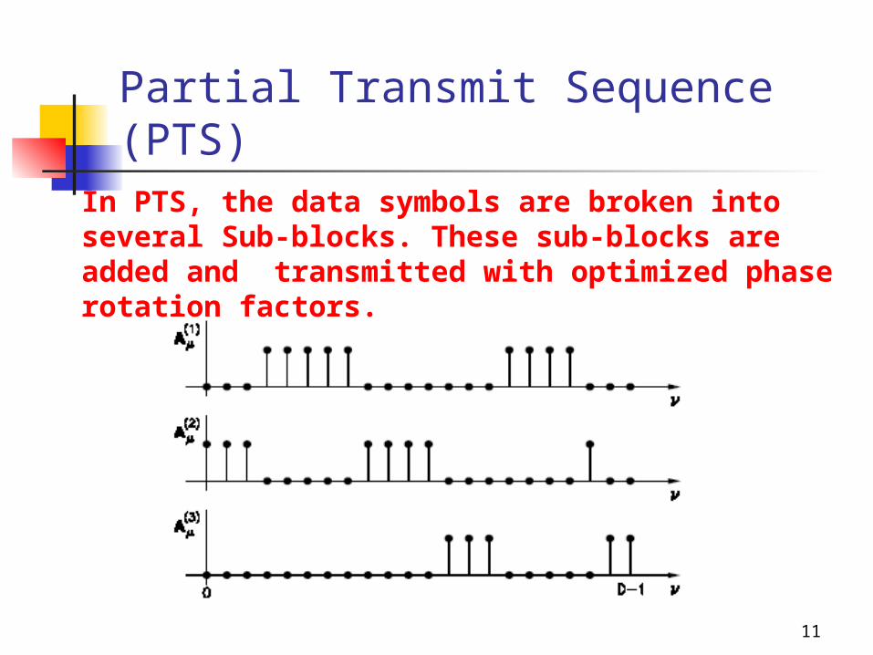
Partial Transmit Sequence (PTS)In PTS, the data symbols are broken into several Sub-blocks. These sub-blocks are added and transmitted with optimized phase rotation factors.

12

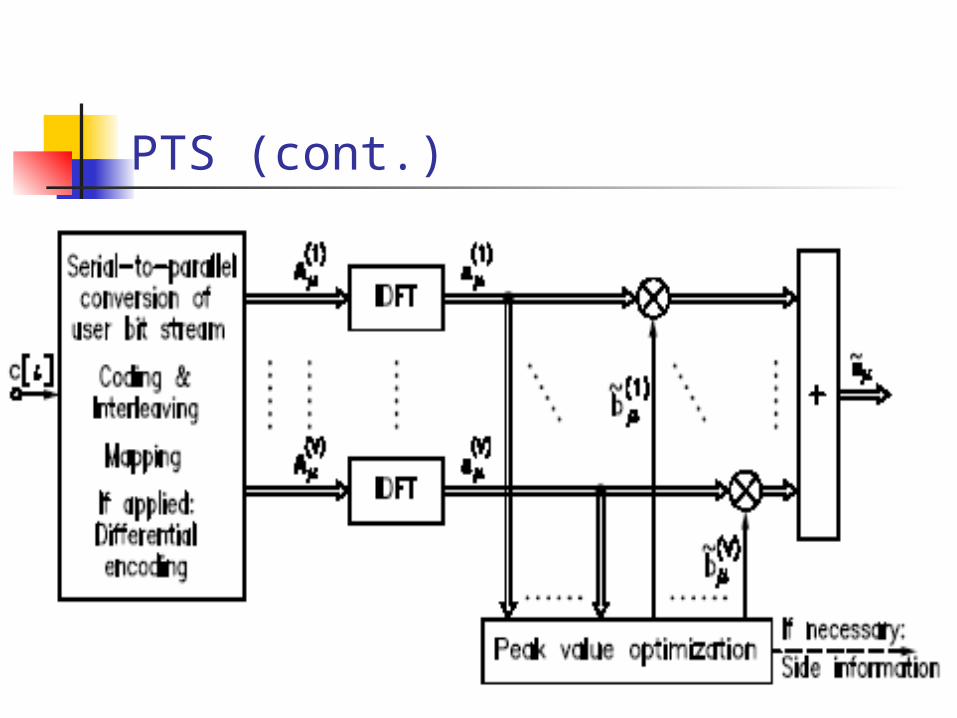
PTS (cont.)

13

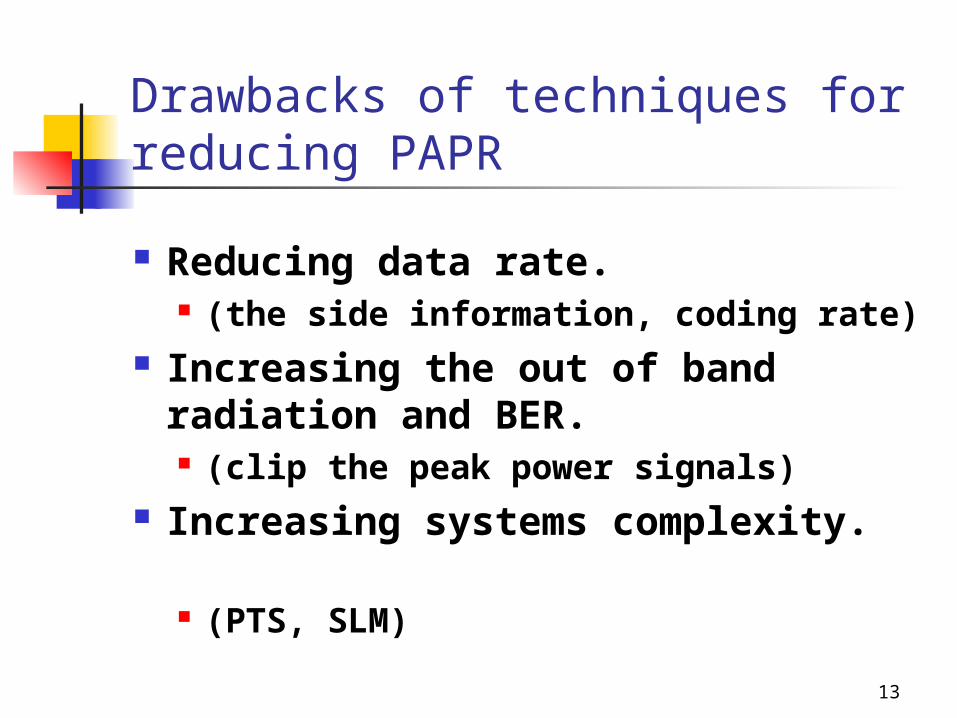
Drawbacks of techniques for reducing PAPR

Reducing data rate.

(the side information, coding rate) Increasing the out of band

radiation and BER. (clip the peak power signals)

Increasing systems complexity.

(PTS, SLM)

14

15

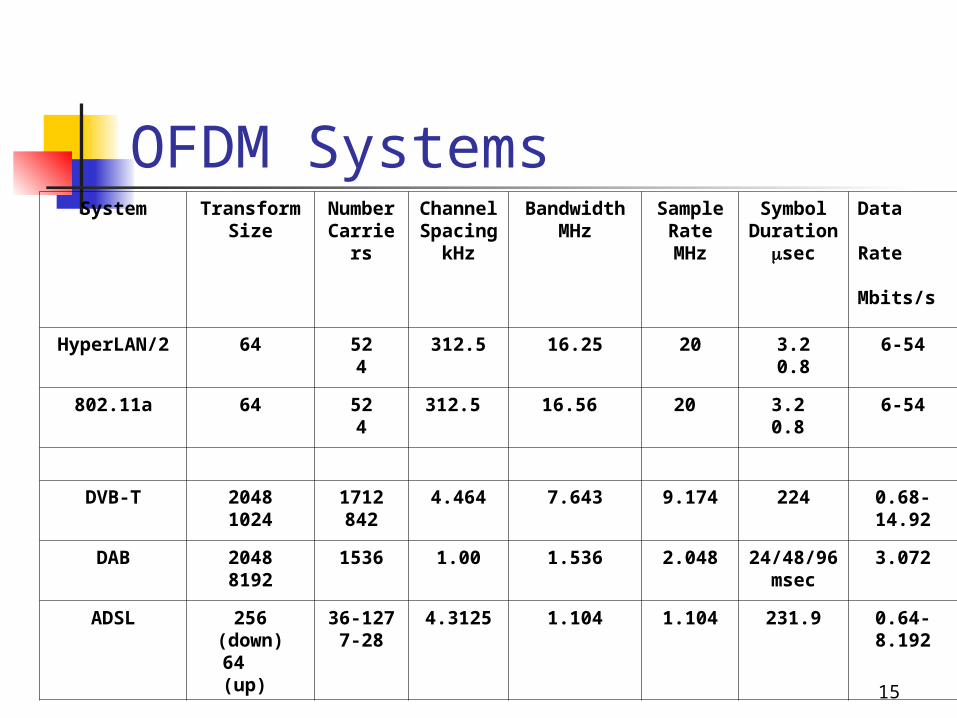
OFDM SystemsSystem Transform

SizeNumberCarriers

ChannelSpacing

kHz

BandwidthMHz

SampleRateMHz

SymbolDuration

sec

Data

Rate

Mbits/s

HyperLAN/2 64 524

312.5 16.25 20 3.20.8

6-54

802.11a 64 524

312.5 16.56 20 3.2 0.8

6-54

DVB-T 20481024

1712842

4.464 7.643 9.174 224 0.68-14.92

DAB 20488192

1536 1.00 1.536 2.048 24/48/96msec

3.072

ADSL 256 (down)64 (up)

36-1277-28

4.3125 1.104 1.104 231.9 0.64-8.192

16

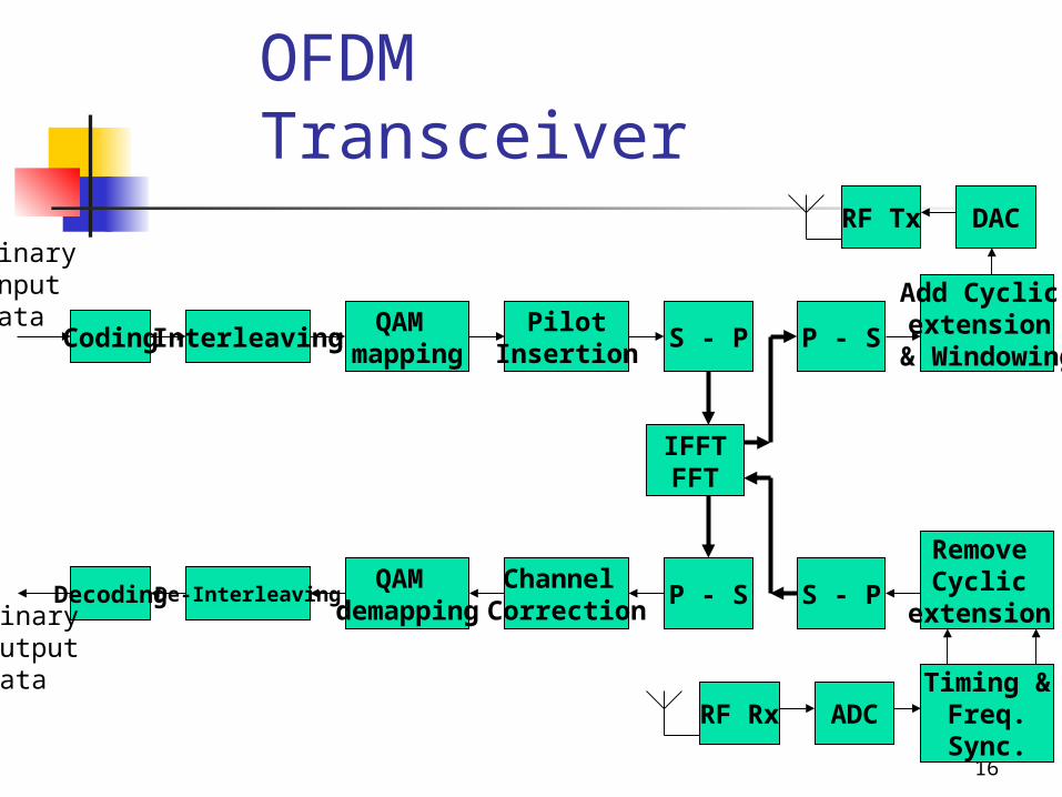
OFDM Transceiver

Coding

Binary Input Data

InterleavingQAM

mappingPilot

InsertionS - P

IFFTFFT

DecodingDe-InterleavingQAM

demappingChannel

CorrectionP - S

Binary Output Data

S - P

P - S

Add Cyclic extension

& Windowing

DACRF Tx

Remove Cyclic

extension

Timing &Freq.Sync.

ADCRF Rx

17

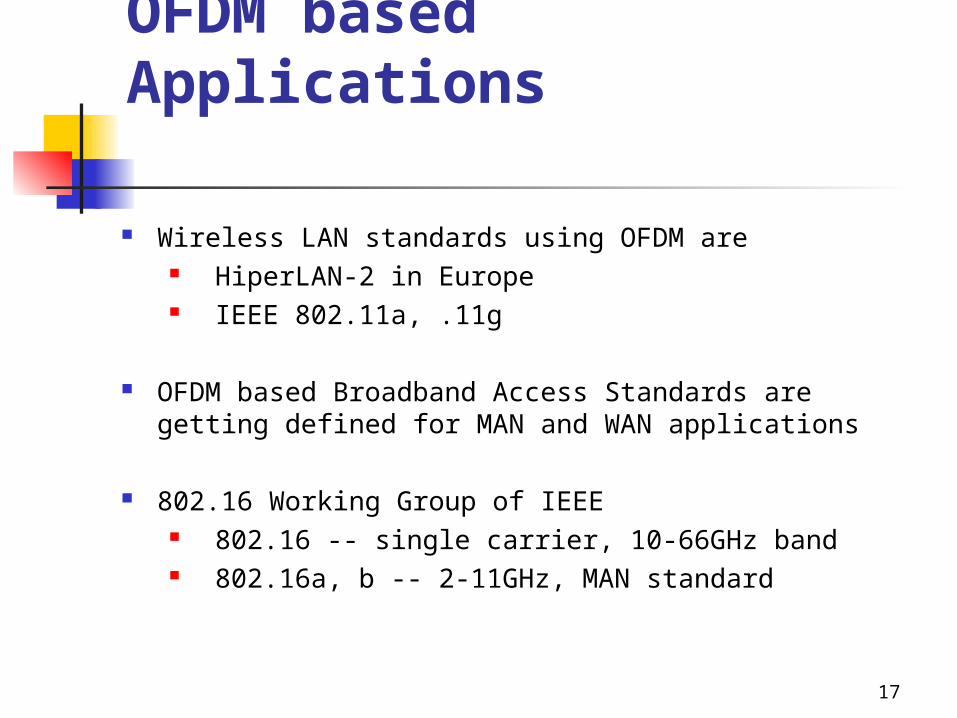
OFDM based Applications

Wireless LAN standards using OFDM are HiperLAN-2 in Europe IEEE 802.11a, .11g

OFDM based Broadband Access Standards are getting defined for MAN and WAN applications

802.16 Working Group of IEEE 802.16 -- single carrier, 10-66GHz band 802.16a, b -- 2-11GHz, MAN standard

18

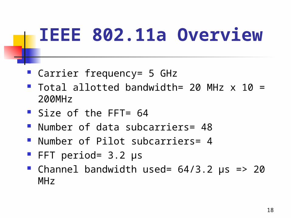
IEEE 802.11a Overview

Carrier frequency= 5 GHz Total allotted bandwidth= 20 MHz x 10 =

200MHz Size of the FFT= 64 Number of data subcarriers= 48 Number of Pilot subcarriers= 4 FFT period= 3.2 µs Channel bandwidth used= 64/3.2 µs => 20

MHz

19

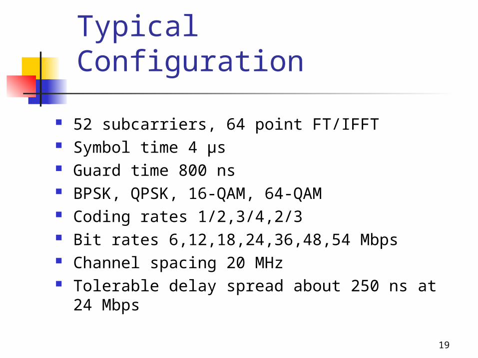
Typical Configuration

52 subcarriers, 64 point FT/IFFT Symbol time 4 µs Guard time 800 ns BPSK, QPSK, 16-QAM, 64-QAM Coding rates 1/2,3/4,2/3 Bit rates 6,12,18,24,36,48,54 Mbps Channel spacing 20 MHz Tolerable delay spread about 250 ns at 24

Mbps

20

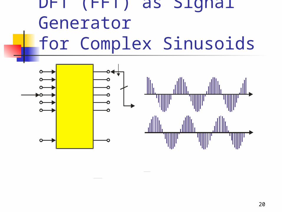
DFT (FFT) as Signal Generatorfor Complex Sinusoids

21

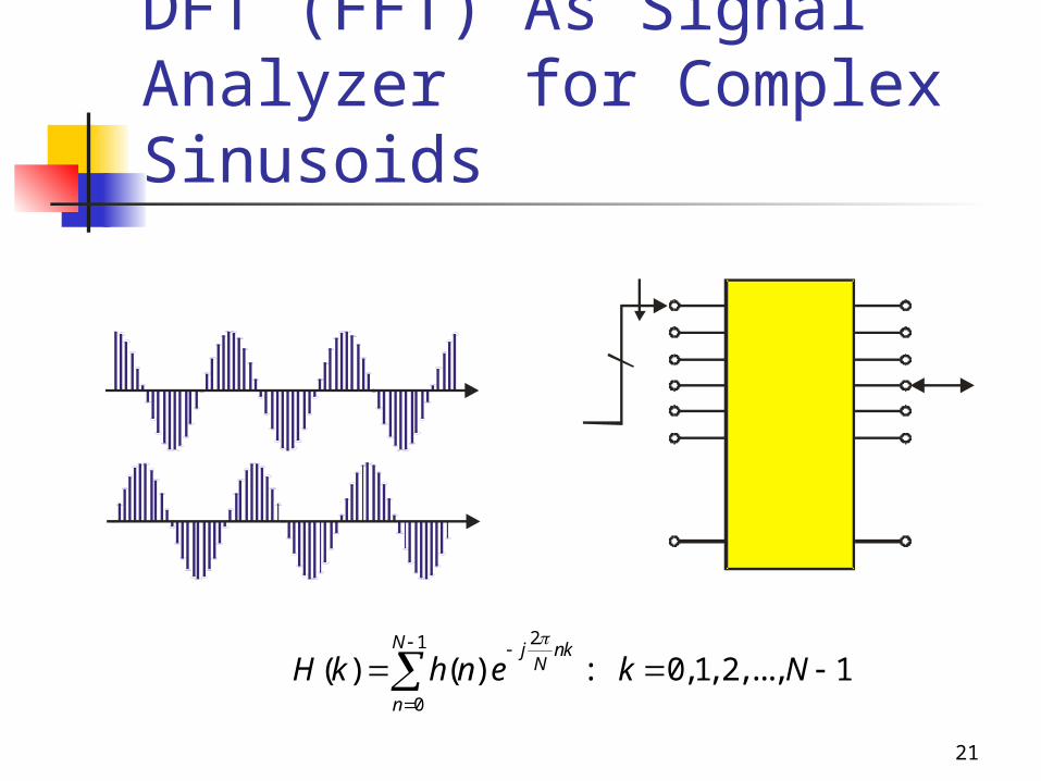
DFT (FFT) As Signal Analyzer for Complex Sinusoids

1,...,2,1,0:)()(1

0

2

NkenhkH

N

n

nkNj

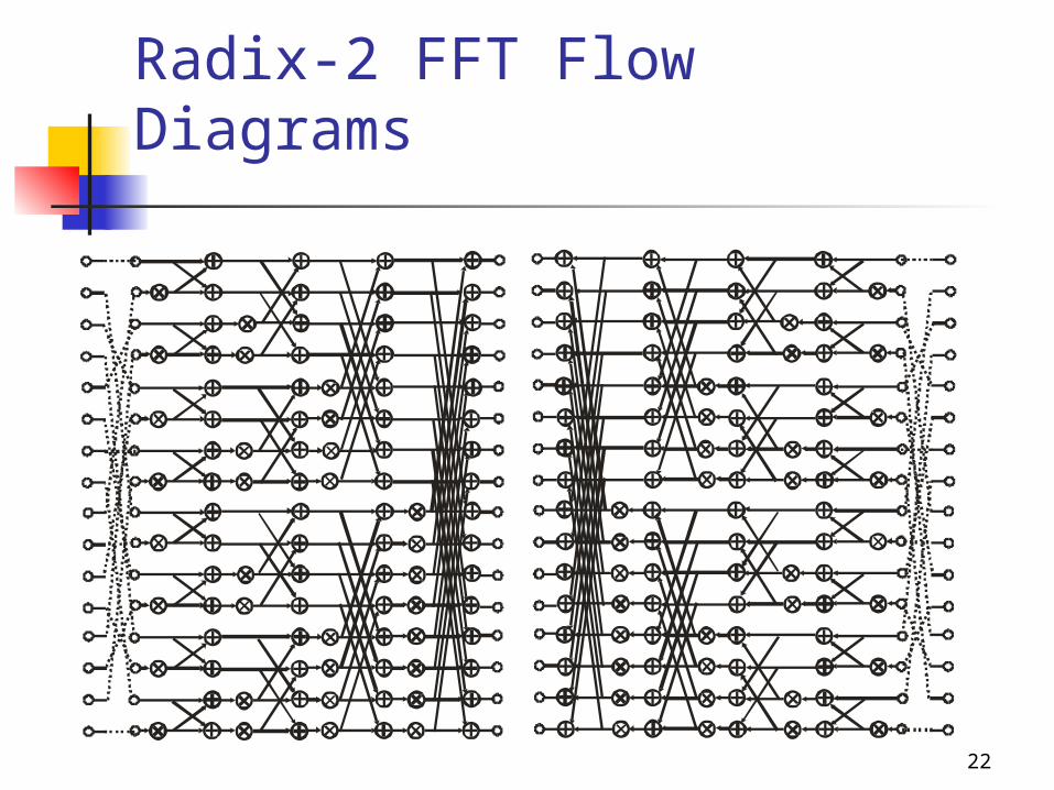
22

Radix-2 FFT Flow Diagrams

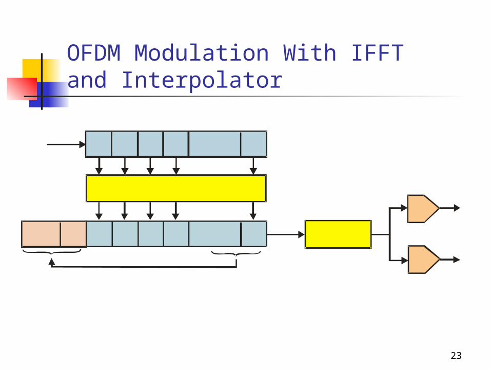
23

OFDM Modulation With IFFTand Interpolator

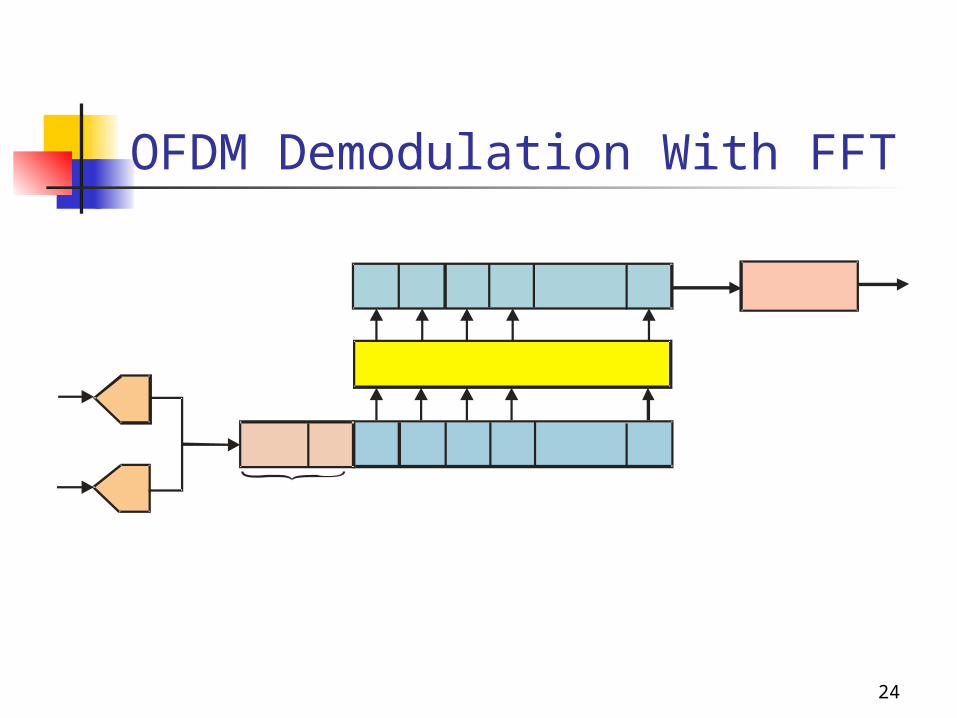
24

OFDM Demodulation With FFT

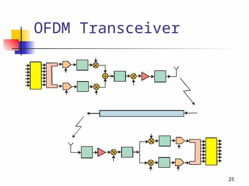
25

OFDM Transceiver

26

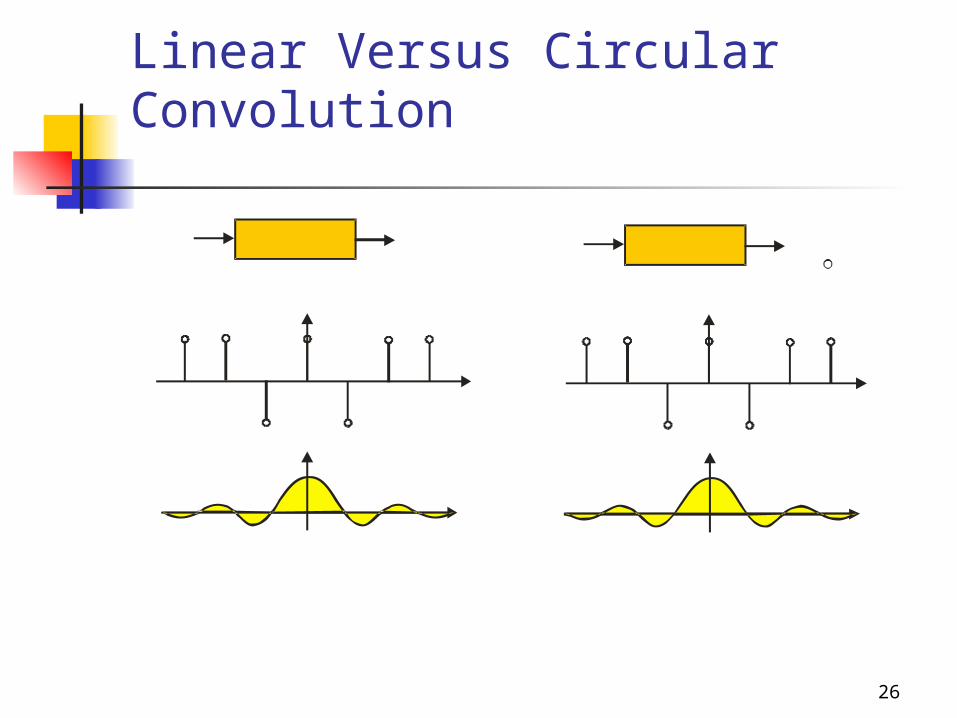
Linear Versus Circular Convolution

27

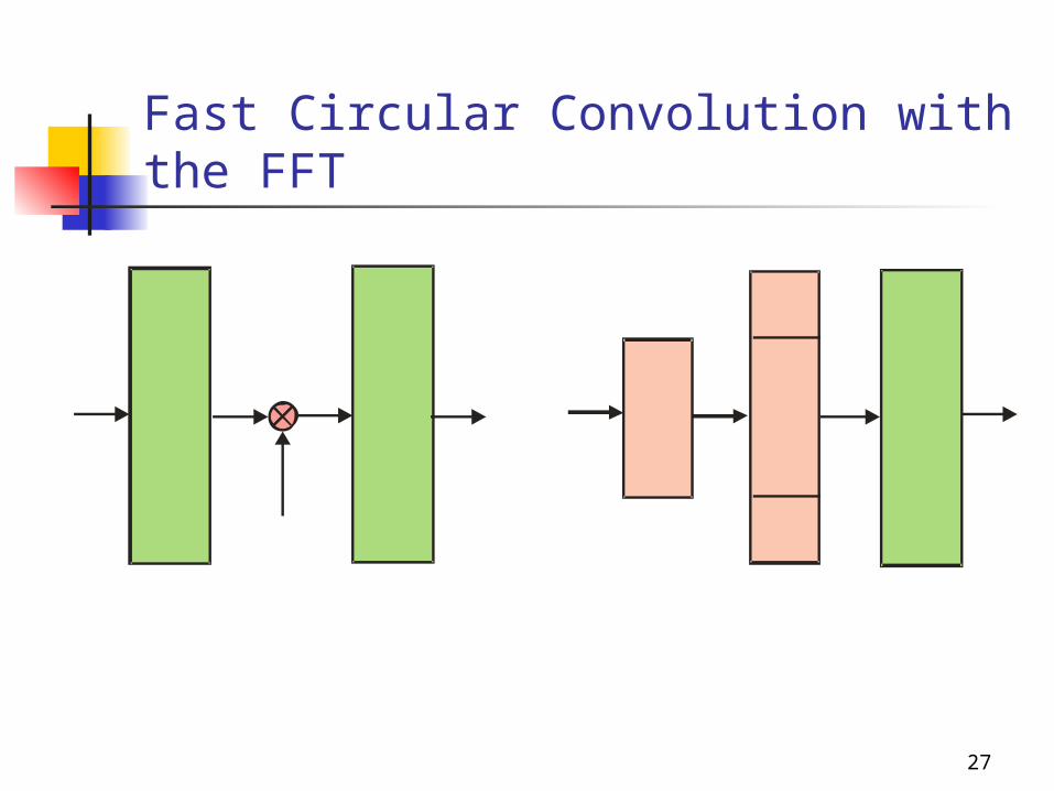
Fast Circular Convolution with the FFT

28

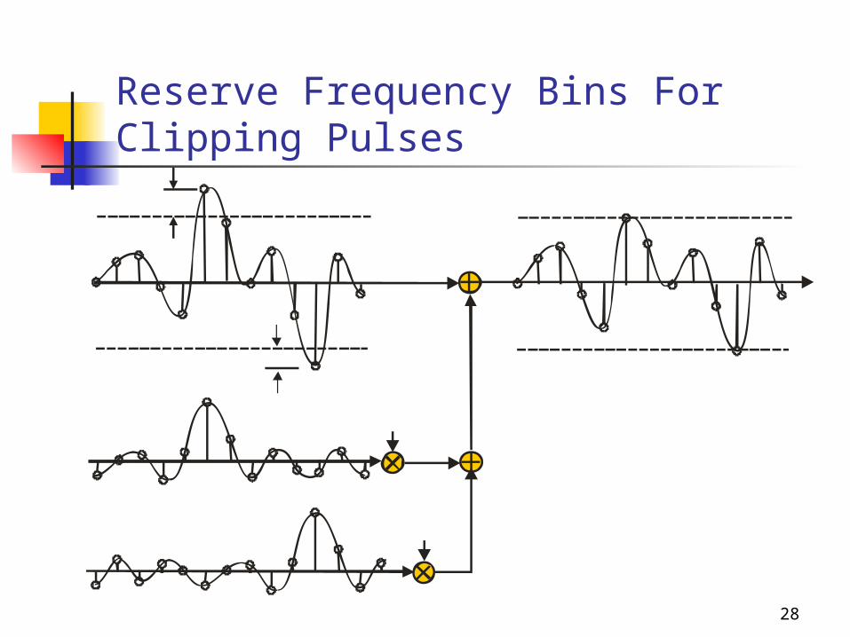
Reserve Frequency Bins For Clipping Pulses

29

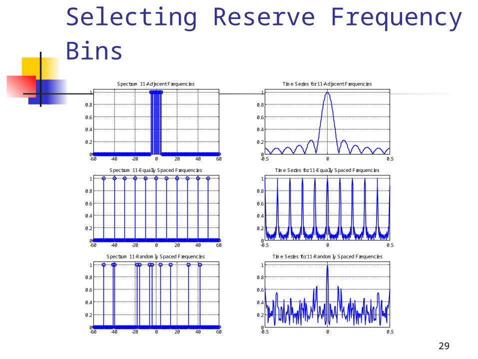
Selecting Reserve Frequency Bins

-60 -40 -20 0 20 40 600

0.2

0.4

0.6

0.8

1

Spectrum 11-Adjacent Frequencies

-0.5 0 0.50

0.2

0.4

0.6

0.8

1

Time Series for 11-Adjacent Frequencies

-60 -40 -20 0 20 40 600

0.2

0.4

0.6

0.8

1

Spectrum 11-Equally Spaced Frequencies

-0.5 0 0.50

0.2

0.4

0.6

0.8

1

Time Series for 11-Equally Spaced Frequencies

-60 -40 -20 0 20 40 600

0.2

0.4

0.6

0.8

1

Spectrum 11-Randomly Spaced Frequencies

-0.5 0 0.50

0.2

0.4

0.6

0.8

1

Time Series for 11-Randomly Spaced Frequencies

30

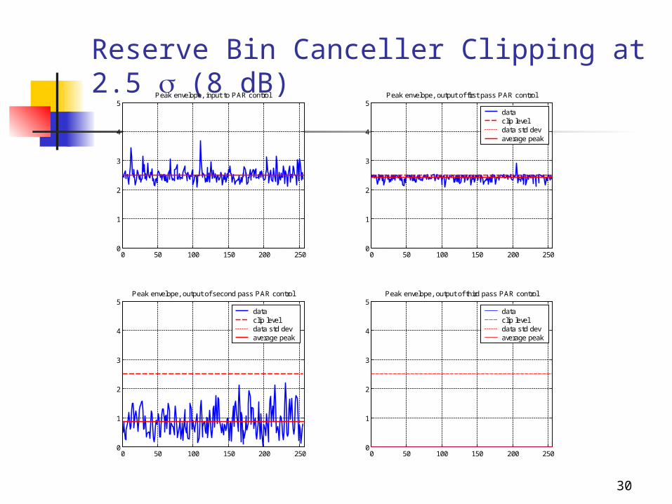
Reserve Bin Canceller Clipping at 2.5 (8 dB)

0 50 100 150 200 2500

1

2

3

4

5Peak envelope, input to PAR control

0 50 100 150 200 2500

1

2

3

4

5Peak envelope, output of first pass PAR control

dataclip leveldata std devaverage peak

0 50 100 150 200 2500

1

2

3

4

5Peak envelope, output of second pass PAR control


0 50 100 150 200 2500

1

2

3

4

5Peak envelope, output of third pass PAR control


31

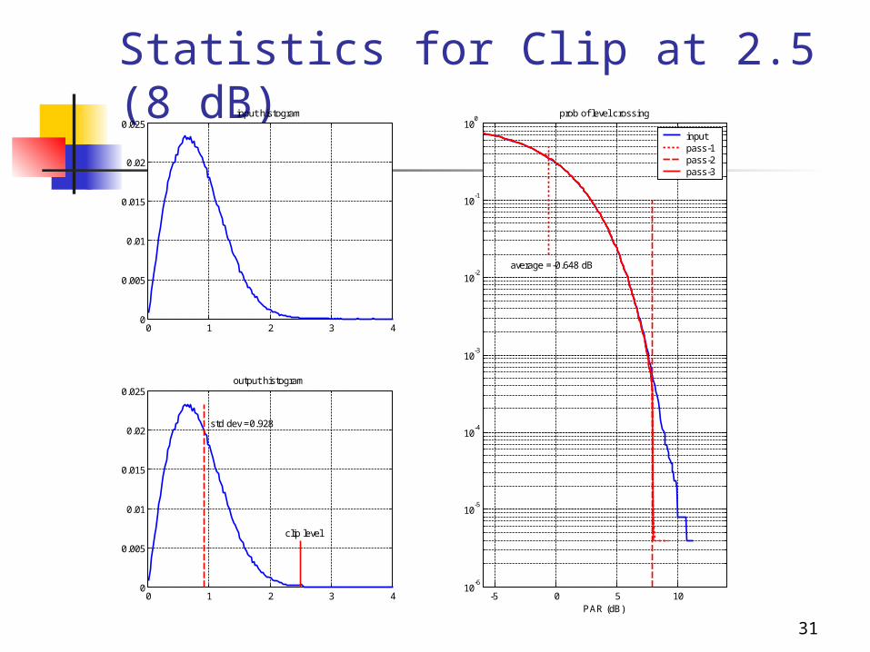
Statistics for Clip at 2.5 (8 dB)

0 1 2 3 40

0.005

0.01

0.015

0.02

0.025input histogram

0 1 2 3 40

0.005

0.01

0.015

0.02

0.025

std dev =0.928

clip level

output histogram

-5 0 5 1010

-6

10-5

10-4

10-3

10-2

10-1

100

average =-0.648 dB

prob of level crossing

PAR (dB)

inputpass-1pass-2pass-3

32

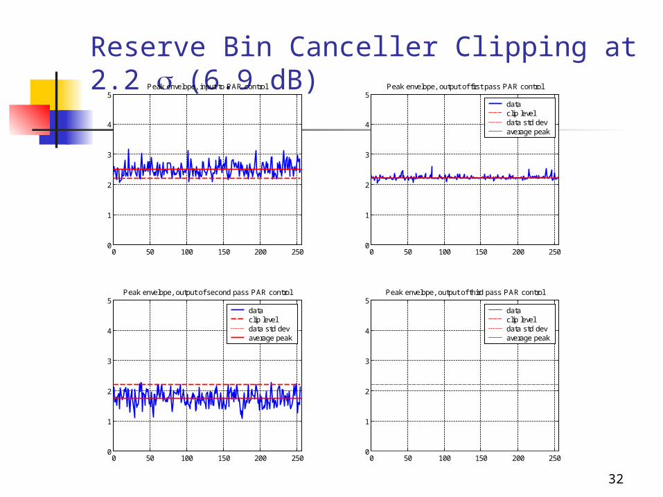
Reserve Bin Canceller Clipping at 2.2 (6.9 dB)

0 50 100 150 200 2500

1

2

3

4


0 50 100 150 200 2500

1

2

3

4



0 50 100 150 200 2500

1

2

3

4



0 50 100 150 200 2500

1

2

3

4



33

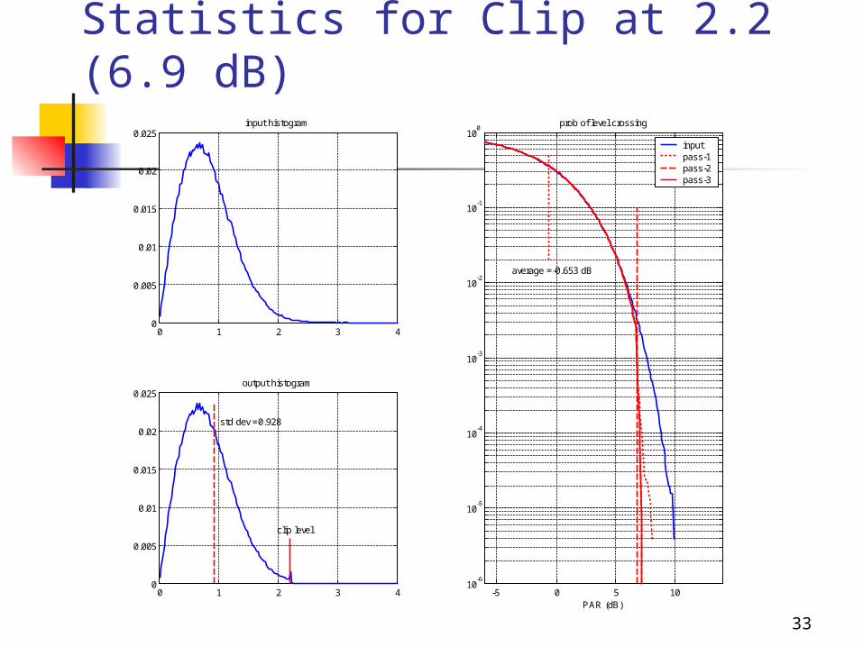
Statistics for Clip at 2.2 (6.9 dB)

0 1 2 3 40

0.005

0.01

0.015

0.02


0 1 2 3 40

0.005

0.01

0.015

0.02

0.025

std dev =0.928

clip level

output histogram

-5 0 5 1010

-6

10-5

10-4

10-3

10-2

10-1

100

average =-0.653 dB


PAR (dB)


34

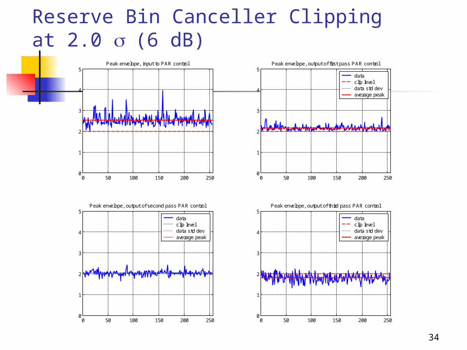
Reserve Bin Canceller Clipping at 2.0 (6 dB)

0 50 100 150 200 2500

1

2

3

4


0 50 100 150 200 2500

1

2

3

4



0 50 100 150 200 2500

1

2

3

4



0 50 100 150 200 2500

1

2

3

4



35

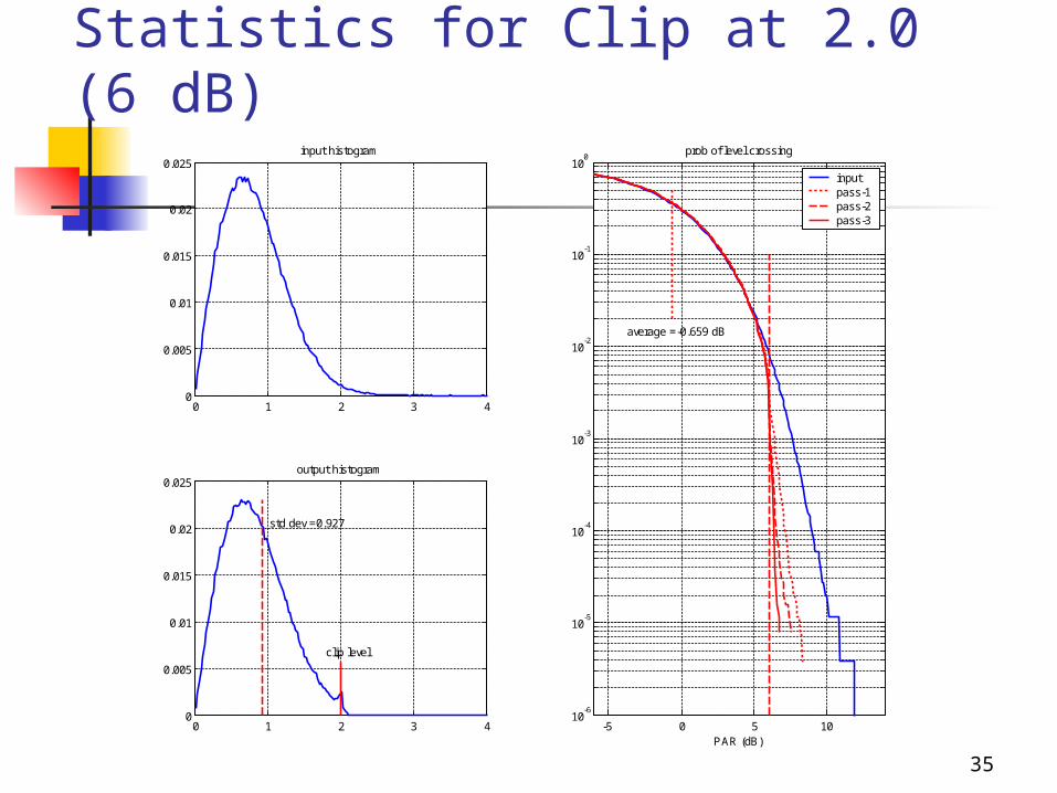
Statistics for Clip at 2.0 (6 dB)

0 1 2 3 40

0.005

0.01

0.015

0.02


0 1 2 3 40

0.005

0.01

0.015

0.02

0.025

std dev =0.927

clip level

output histogram

-5 0 5 1010

-6

10-5

10-4

10-3

10-2

10-1

100

average =-0.659 dB


PAR (dB)


Documents

1 Peak-to-Average Power Ratio (PAPR) One of the main problems in OFDM system is large PAPR /PAR(increased complexity of the ADC and DAC, and reduced efficiency