1

Pertemua 19 Regresi Linier

:

2

Outline Materi : Koefisien korelasi dan determinasi Persamaan regresi Regresi dan peramalan

3

Simple Correllation and Linear Regression

• Types of Regression Models

• Determining the Simple Linear Regression Equation

• Measures of Variation

• Assumptions of Regression and Correlation

• Residual Analysis

• Measuring Autocorrelation

• Inferences about the Slope

4

Simple Correlation and…

• Correlation - Measuring the Strength of the Association

• Estimation of Mean Values and Prediction of Individual Values

• Pitfalls in Regression and Ethical Issues

(continued)

5

Purpose of Regression Analysis

• Regression Analysis is Used Primarily to Model Causality and Provide Prediction– Predict the values of a dependent (response)

variable based on values of at least one independent (explanatory) variable

– Explain the effect of the independent variables on the dependent variable

6

Types of Regression Models

Positive Linear Relationship

Negative Linear Relationship

Relationship NOT Linear

No Relationship

7

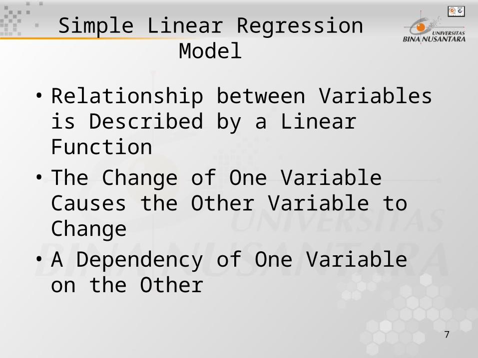
Simple Linear Regression Model

• Relationship between Variables is Described by a Linear Function

• The Change of One Variable Causes the Other Variable to Change

• A Dependency of One Variable on the Other

8

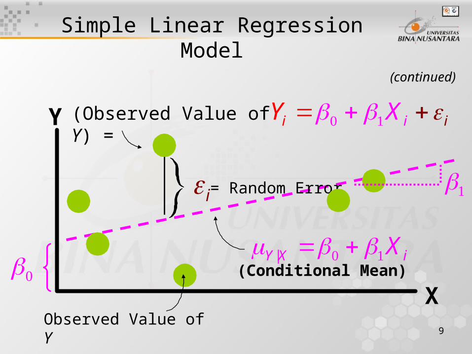
PopulationRegressionLine (Conditional Mean)

Simple Linear Regression Model

Population regression line is a straight line that describes the dependence of the average value (conditional mean)average value (conditional mean) of one variable on the other

Population Y Intercept

Population SlopeCoefficient

Random Error

Dependent (Response) Variable

Independent (Explanatory) Variable

ii iY X

|Y X

(continued)

9

Simple Linear Regression Model

(continued)

ii iY X

= Random Error

Y

X

(Observed Value of Y) =

Observed Value of Y

|Y X iX

i

(Conditional Mean)

10

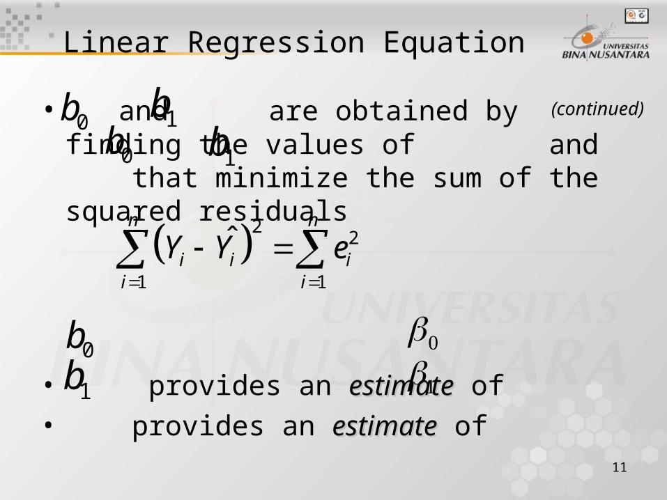
Sample regression line provides an estimateestimate of the population regression line as well as a predicted value of Y

Linear Regression Equation

Sample Y Intercept

SampleSlopeCoefficient

Residual0 1i iib bY X e

0 1Y b b X Simple Regression Equation (Fitted Regression Line, Predicted Value)

11

Linear Regression Equation

• and are obtained by finding the values of and that minimize the sum of the squared residuals

• provides an estimateestimate of

• provides an estimateestimate of

0b 1b0b 1b

0b

1b

(continued)

22

1 1

ˆn n

i i ii i

Y Y e

12

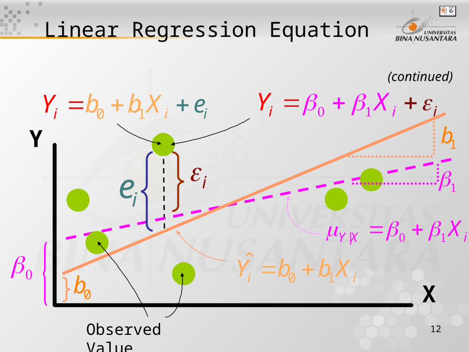
Linear Regression Equation

(continued)

Y

XObserved Value

|Y X iX

i

ii iY X

0 1i iY b b X

ie

0 1i iib bY X e 1b

0b

13

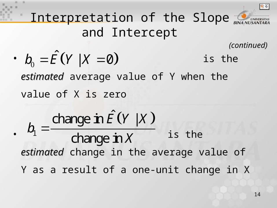
Interpretation of the Slopeand Intercept

• is the average value of Y

when the value of X is zero

• measures the

change in the average value of Y as a

result of a one-unit change in X

| 0E Y X

1

change in |

change in

E Y X

X

14

Interpretation of the Slopeand Intercept

• is the estimatedestimated average

value of Y when the value of X is zero

• is the

estimatedestimated change in the average value of Y

as a result of a one-unit change in X

(continued)

ˆ | 0b E Y X

1

ˆchange in |

change in

E Y Xb

X

15

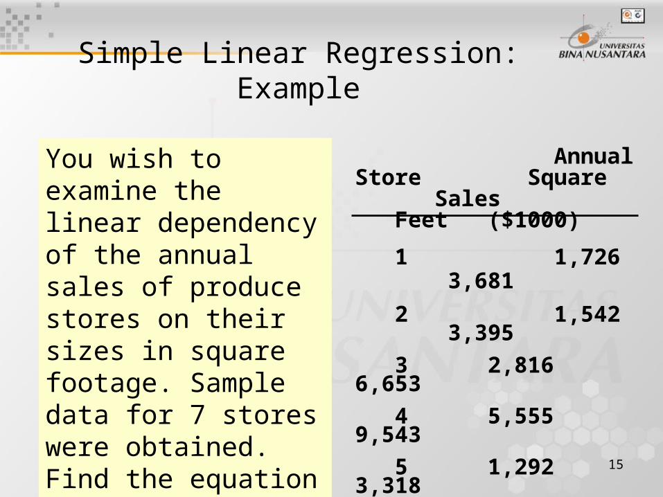
Simple Linear Regression: Example

You wish to examine the linear dependency of the annual sales of produce stores on their sizes in square footage. Sample data for 7 stores were obtained. Find the equation of the straight line that fits the data best.

Annual Store Square Sales

Feet ($1000)

1 1,726 3,681

2 1,542 3,395

3 2,816 6,653

4 5,555 9,543

5 1,292 3,318

6 2,208 5,563

7 1,313 3,760

16

Scatter Diagram: Example

0

2000

4000

6000

8000

10000

12000

0 1000 2000 3000 4000 5000 6000

Square Feet

An

nu

al

Sa

les

($00

0)

Excel Output

17

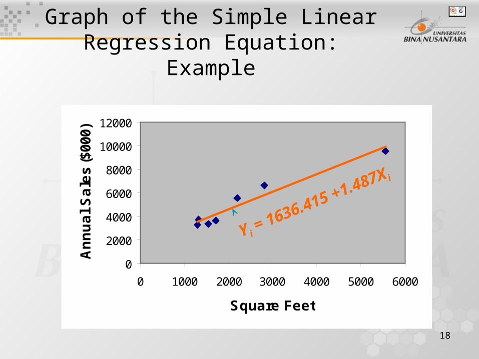
Simple Linear Regression Equation: Example

0 1ˆ

1636.415 1.487i i

i

Y b b X

X

From Excel Printout:

CoefficientsIntercept 1636.414726X Variable 1 1.486633657

18

Graph of the Simple Linear Regression Equation: Example

0

2000

4000

6000

8000

10000

12000

0 1000 2000 3000 4000 5000 6000

Square Feet

An

nu

al

Sa

les

($00

0)

Y i = 1636.415 +1.487X i

19

Interpretation of Results: Example

The slope of 1.487 means that for each increase of one unit in X, we predict the average of Y to increase by an estimated 1.487 units.

The equation estimates that for each increase of 1 square foot in the size of the store, the expected annual sales are predicted to increase by $1487.

ˆ 1636.415 1.487i iY X

20

Simple Linear Regressionin PHStat

• In Excel, use PHStat | Regression | Simple Linear Regression …

• Excel Spreadsheet of Regression Sales on Footage

Microsoft Excel Worksheet

21

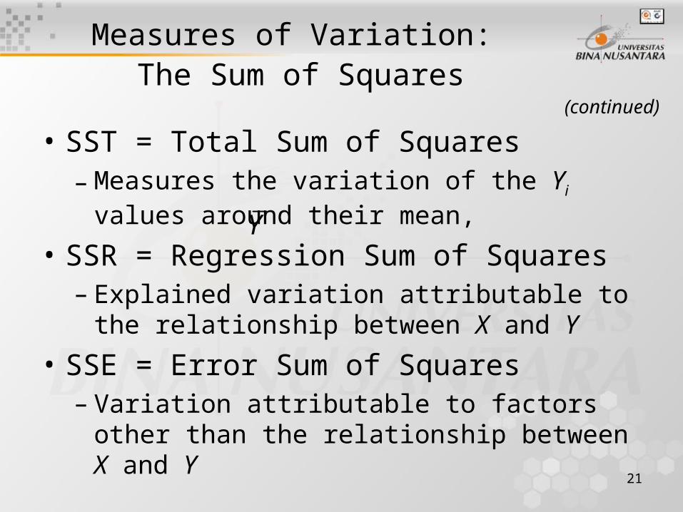
Measures of Variation: The Sum of Squares

• SST = Total Sum of Squares – Measures the variation of the Yi values

around their mean,

• SSR = Regression Sum of Squares – Explained variation attributable to the

relationship between X and Y

• SSE = Error Sum of Squares – Variation attributable to factors other than the

relationship between X and Y

(continued)

Y

22

The Coefficient of Determination

•

• Measures the proportion of variation in Y that is explained by the independent variable X in the regression model

2 Regression Sum of Squares

Total Sum of Squares

SSRr

SST

23

Venn Diagrams and Explanatory Power of Regression

Sales

Sizes

2

SSR

SSR S

r

SE

24

Coefficients of Determination (r 2) and Correlation (r)

r2 = 1, r2 = 1,

r2 = .81, r2 = 0,Y

Yi = b0 + b1Xi

X

^

YYi = b0 + b1Xi

X

^Y

Yi = b0 + b1 X i

X

^

Y

Yi = b0 + b1Xi

X

^

r = +1 r = -1

r = +0.9 r = 0

25

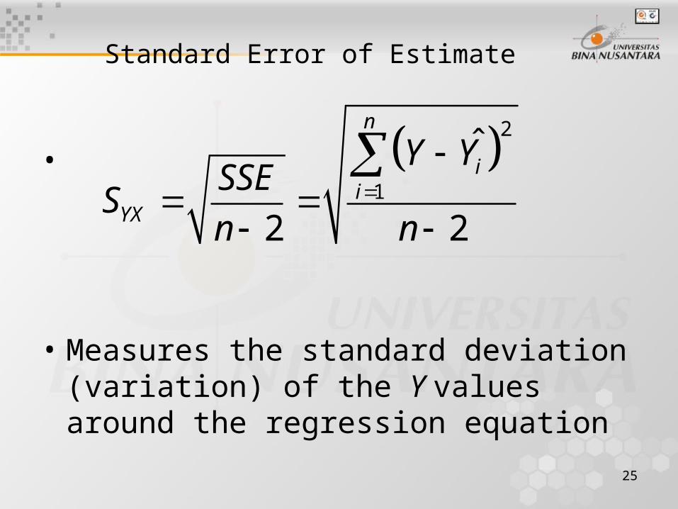
Standard Error of Estimate

•

• Measures the standard deviation (variation) of the Y values around the regression equation

2

1

ˆ

2 2

n

ii

YX

Y YSSE

Sn n

26

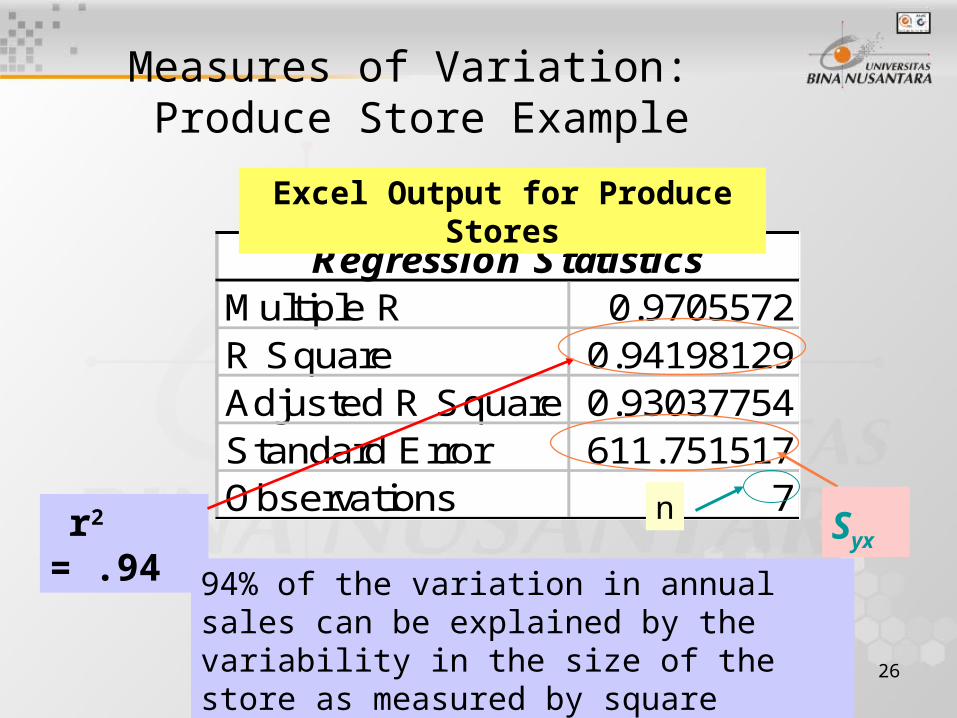
Measures of Variation: Produce Store Example

Regression StatisticsMultiple R 0.9705572R Square 0.94198129Adjusted R Square 0.93037754Standard Error 611.751517Observations 7

Excel Output for Produce Stores

r2 = .94

94% of the variation in annual sales can be explained by the variability in the size of the store as measured by square footage.

Syxn

27

Linear Regression Assumptions

• Normality– Y values are normally distributed for each X– Probability distribution of error is normal

• Homoscedasticity (Constant Variance)

• Independence of Errors

28

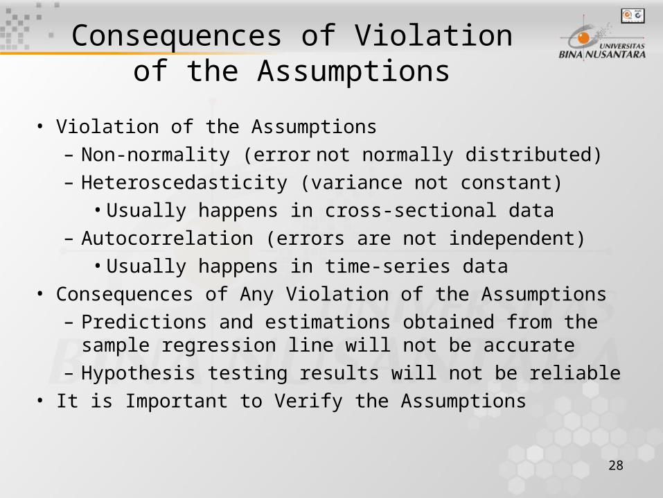
Consequences of Violationof the Assumptions

• Violation of the Assumptions– Non-normality (error not normally distributed)– Heteroscedasticity (variance not constant)

• Usually happens in cross-sectional data– Autocorrelation (errors are not independent)

• Usually happens in time-series data• Consequences of Any Violation of the Assumptions

– Predictions and estimations obtained from the sample regression line will not be accurate

– Hypothesis testing results will not be reliable• It is Important to Verify the Assumptions

29

• Y values are normally distributed around the regression line.

• For each X value, the “spread” or variance around the regression line is the same.

Variation of Errors Aroundthe Regression Line

X1

X2

X

Y

f(e)

Sample Regression Line

30

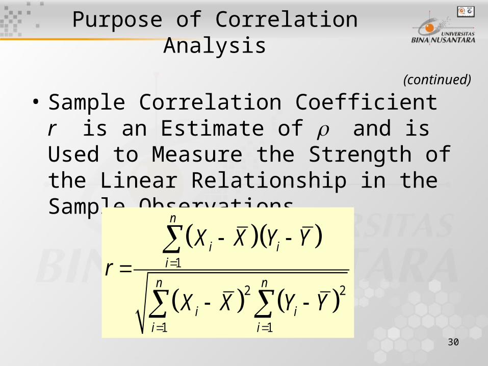
• Sample Correlation Coefficient r is an Estimate of and is Used to Measure the Strength of the Linear Relationship in the Sample Observations

Purpose of Correlation Analysis(continued)

1

2 2

1 1

n

i ii

n n

i ii i

X X Y Yr

X X Y Y

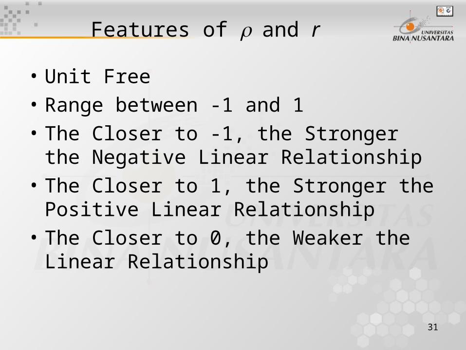
31

Features of and r

• Unit Free

• Range between -1 and 1

• The Closer to -1, the Stronger the Negative Linear Relationship

• The Closer to 1, the Stronger the Positive Linear Relationship

• The Closer to 0, the Weaker the Linear Relationship

32

Pitfalls of Regression Analysis

• Lacking an Awareness of the Assumptions Underlining Least-Squares Regression

• Not Knowing How to Evaluate the Assumptions

• Not Knowing What the Alternatives to Least-Squares Regression are if a Particular Assumption is Violated

• Using a Regression Model Without Knowledge of the Subject Matter

33

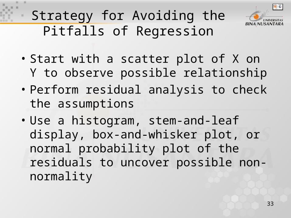
Strategy for Avoiding the Pitfalls of Regression

• Start with a scatter plot of X on Y to observe possible relationship

• Perform residual analysis to check the assumptions

• Use a histogram, stem-and-leaf display, box-and-whisker plot, or normal probability plot of the residuals to uncover possible non-normality

34

Strategy for Avoiding the Pitfalls of Regression

• If there is violation of any assumption, use alternative methods (e.g., least absolute deviation regression or least median of squares regression) to least-squares regression or alternative least-squares models (e.g., curvilinear or multiple regression)

• If there is no evidence of assumption violation, then test for the significance of the regression coefficients and construct confidence intervals and prediction intervals

(continued)

35

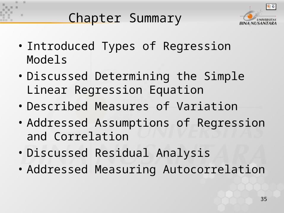
Chapter Summary

• Introduced Types of Regression Models

• Discussed Determining the Simple Linear Regression Equation

• Described Measures of Variation

• Addressed Assumptions of Regression and Correlation

• Discussed Residual Analysis

• Addressed Measuring Autocorrelation

36

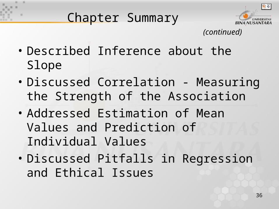
Chapter Summary

• Described Inference about the Slope

• Discussed Correlation - Measuring the Strength of the Association

• Addressed Estimation of Mean Values and Prediction of Individual Values

• Discussed Pitfalls in Regression and Ethical Issues

(continued)