1

Peter Fox

Data Analytics – ITWS-4963/ITWS-6965

Week 11a, April 14, 2015

Interpreting cross-validation, bootstrapping, bagging,

boosting, etc.

coleman> head(coleman)

salaryP fatherWc sstatus teacherSc motherLev Y

1 3.83 28.87 7.20 26.6 6.19 37.01

2 2.89 20.10 -11.71 24.4 5.17 26.51

3 2.86 69.05 12.32 25.7 7.04 36.51

4 2.92 65.40 14.28 25.7 7.10 40.70

5 3.06 29.59 6.31 25.4 6.15 37.10

6 2.07 44.82 6.16 21.6 6.41 33.90

2

What were you doing?> call <- call("lmrob", formula = Y ~ .)

> # set up folds for cross-validation

> folds <- cvFolds(nrow(coleman), K = 5, R = 10)

> # perform cross-validation

> cvTool(call, data = coleman, y = coleman$Y, cost = rtmspe,

+ folds = folds, costArgs = list(trim = 0.1))

CV

[1,] 0.9880672

[2,] 0.9525881

[3,] 0.8989264

[4,] 1.0177694

[5,] 0.9860661

[6,] 1.8369717

[7,] 0.9550428

[8,] 1.0698466

[9,] 1.3568537

[10,] 0.8313474

3

Warning messages:1: In lmrob.S(x, y, control = control) : S refinements did not converge (to refine.tol=1e-07) in 200 (= k.max) steps2: In lmrob.S(x, y, control = control) : S refinements did not converge (to refine.tol=1e-07) in 200 (= k.max) steps3: In lmrob.S(x, y, control = control) : find_scale() did not converge in 'maxit.scale' (= 200) iterations4: In lmrob.S(x, y, control = control) : find_scale() did not converge in 'maxit.scale' (= 200) iterations

Did you get this plot – how?> cvFits

5-fold CV results:

Fit CV

1 LS 1.674485

2 MM 1.147130

3 LTS 1.291797

Best model:

CV

"MM"

4

LS, LTS, MM?• The breakdown value of an estimator is defined as

the smallest fraction of contamination that can cause the estimator to take on values arbitrarily far from its value on the uncontaminated data.

• The breakdown value of an estimator can be used as a measure of the robustness of the estimator. Rousseeuw and Leroy (1987) and others introduced high breakdown value estimators for linear regression.

• LTS – see http://support.sas.com/documentation/cdl/en/statug/63033/HTML/default/viewer.htm#statug_rreg_sect018.htm#statug.rreg.robustregfltsest

• MM - http://support.sas.com/documentation/cdl/en/statug/63033/HTML/default/viewer.htm#statug_rreg_sect019.htm

5

50 and 75% subsetsfitLts50 <- ltsReg(Y ~ ., data = coleman, alpha = 0.5)

cvFitLts50 <- cvLts(fitLts50, cost = rtmspe, folds = folds,

fit = "both", trim = 0.1)

# 75% subsets

fitLts75 <- ltsReg(Y ~ ., data = coleman, alpha = 0.75)

cvFitLts75 <- cvLts(fitLts75, cost = rtmspe, folds = folds,

fit = "both", trim = 0.1)

# combine and plot results

cvFitsLts <- cvSelect("0.5" = cvFitLts50, "0.75" = cvFitLts75)

6

cvFitsLts (50/75)> cvFitsLts

5-fold CV results:

Fit reweighted raw

1 0.5 1.291797 1.640922

2 0.75 1.065495 1.232691

Best model:

reweighted raw

"0.75" "0.75"

7

Tuningtuning <- list(tuning.psi=c(3.14, 3.44, 3.88, 4.68))

# perform cross-validation

cvFitsLmrob <- cvTuning(fitLmrob$call, data = coleman, y = coleman$Y, tuning = tuning, cost = rtmspe, folds = folds, costArgs = list(trim = 0.1))

8

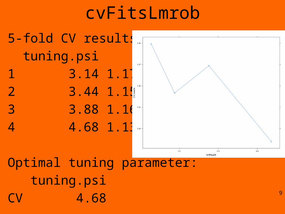
cvFitsLmrob5-fold CV results:

tuning.psi CV

1 3.14 1.179620

2 3.44 1.156674

3 3.88 1.169436

4 4.68 1.133975

Optimal tuning parameter:

tuning.psi

CV 4.68 9

Lab on Fridaymammals.glm <- glm(log(brain) ~ log(body), data = mammals)

(cv.err <- cv.glm(mammals, mammals.glm)$delta)

[1] 0.4918650 0.4916571

> (cv.err.6 <- cv.glm(mammals, mammals.glm, K = 6)$delta)

[1] 0.4967271 0.4938003

# As this is a linear model we could calculate the leave-one-out

# cross-validation estimate without any extra model-fitting.

muhat <- fitted(mammals.glm)

mammals.diag <- glm.diag(mammals.glm)

(cv.err <- mean((mammals.glm$y - muhat)^2/(1 - mammals.diag$h)^2))

[1] 0.491865 10

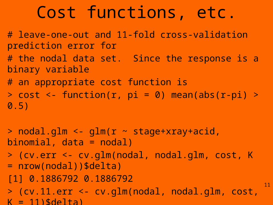
Cost functions, etc.# leave-one-out and 11-fold cross-validation prediction error for

# the nodal data set. Since the response is a binary variable

# an appropriate cost function is

> cost <- function(r, pi = 0) mean(abs(r-pi) > 0.5)

> nodal.glm <- glm(r ~ stage+xray+acid, binomial, data = nodal)

> (cv.err <- cv.glm(nodal, nodal.glm, cost, K = nrow(nodal))$delta)

[1] 0.1886792 0.1886792

> (cv.11.err <- cv.glm(nodal, nodal.glm, cost, K = 11)$delta)

[1] 0.2264151 0.2228551

11

cvTools• http://cran.r-project.org/web/packages/cvTool

s/cvTools.pdf

• Very powerful and flexible package for CV (regression) but very much a black box!

• If you use it, become very, very familiar with the outputs and be prepared to experiment…

12

Bootstrap aggregation (bagging)

• Improve the stability and accuracy of machine learning algorithms used in statistical classification and regression.

• Also reduces variance and helps to avoid overfitting.

• Usually applied to decision tree methods, but can be used with any type of method.– Bagging is a special case of the model averaging

approach.• Harder to interpret – why?

13

Ozone

14

10 of 100 bootstrap samplesaverage

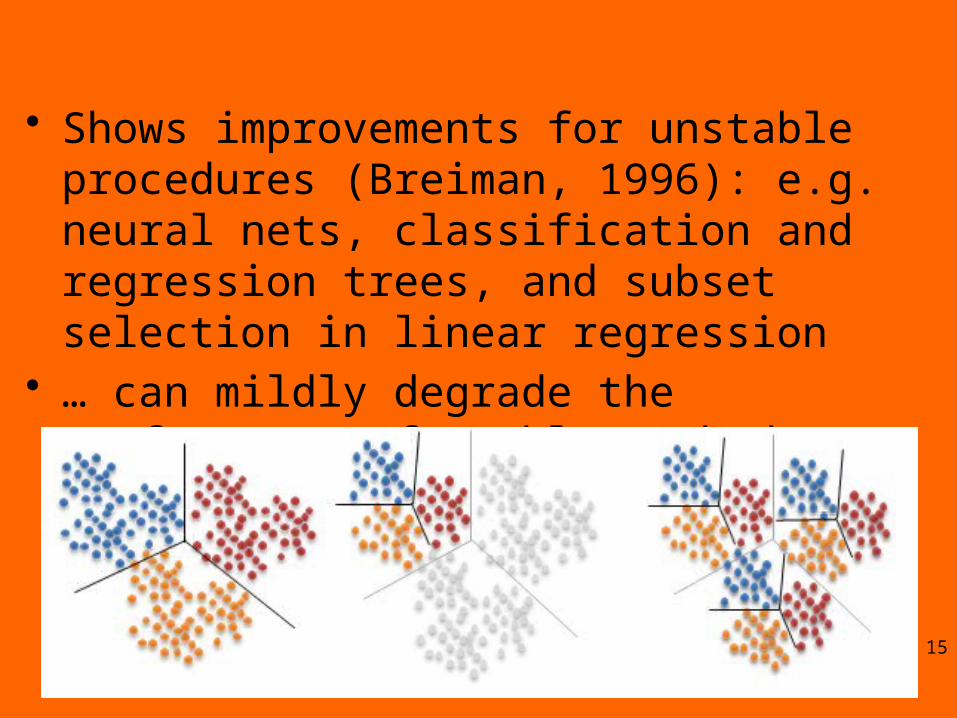
• Shows improvements for unstable procedures (Breiman, 1996): e.g. neural nets, classification and regression trees, and subset selection in linear regression

• … can mildly degrade the performance of stable methods such as K-nearest neighbors

15

Bagging (bootstrapping aggregation)*

library(mlbench)

data(BreastCancer)

l <- length(BreastCancer[,1])

sub <- sample(1:l,2*l/3)

BC.bagging <- bagging(Class ~., data=BreastCancer[,-1], mfinal=20, control=rpart.control(maxdepth=3))

BC.bagging.pred <-predict.bagging( BC.bagging, newdata=BreastCancer[-sub,-1])

BC.bagging.pred$confusion

Observed Class

Predicted Class benign malignant

benign 142 2

malignant 8 81 16

BC.bagging.pred$error[1] 0.04291845

A little later> data(BreastCancer)

> l <- length(BreastCancer[,1])

> sub <- sample(1:l,2*l/3)

> BC.bagging <- bagging(Class ~.,data=BreastCancer[,-1],mfinal=20,

+ control=rpart.control(maxdepth=3))

> BC.bagging.pred <- predict.bagging(BC.bagging,newdata=BreastCancer[-sub,-1])

> BC.bagging.pred$confusion

Observed Class

Predicted Class benign malignant

benign 147 1

malignant 7 78

> BC.bagging.pred$error

[1] 0.03433476

17

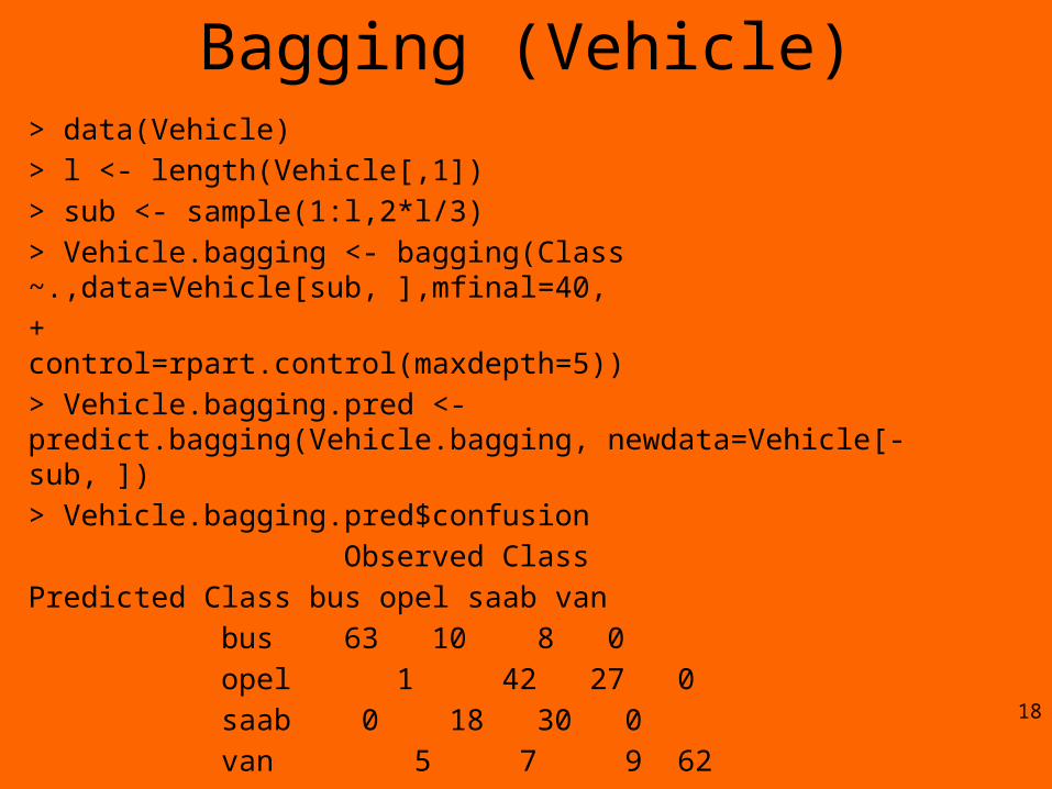
Bagging (Vehicle)> data(Vehicle)

> l <- length(Vehicle[,1])

> sub <- sample(1:l,2*l/3)

> Vehicle.bagging <- bagging(Class ~.,data=Vehicle[sub, ],mfinal=40,

+ control=rpart.control(maxdepth=5))

> Vehicle.bagging.pred <- predict.bagging(Vehicle.bagging, newdata=Vehicle[-sub, ])

> Vehicle.bagging.pred$confusion

Observed Class

Predicted Class bus opel saab van

bus 63 10 8 0

opel 1 42 27 0

saab 0 18 30 0

van 5 7 9 62

> Vehicle.bagging.pred$error

[1] 0.301418418

Weak models …• A weak learner: a classifier which is only

slightly correlated with the true classification (it can label examples better than random guessing)

• A strong learner: a classifier that is arbitrarily well-correlated with the true classification.

• Can a set of weak learners create a single strong learner?

19

Boosting• … reducing bias in supervised learning• most boosting algorithms consist of iteratively

learning weak classifiers with respect to a distribution and adding them to a final strong classifier. – typically weighted in some way that is usually related to

the weak learners' accuracy.

• After a weak learner is added, the data is reweighted: examples that are misclassified gain weight and examples that are classified correctly lose weight

• Thus, future weak learners focus more on the examples that previous weak learners misclassified.

20

Diamonds require(ggplot2) # or load package first

data(diamonds)

head(diamonds) # look at the data!

#

ggplot(diamonds, aes(clarity, fill=cut)) + geom_bar()

ggplot(diamonds, aes(clarity)) + geom_bar() + facet_wrap(~ cut)

ggplot(diamonds) + geom_histogram(aes(x=price)) + geom_vline(xintercept=12000)

ggplot(diamonds, aes(clarity)) + geom_freqpoly(aes(group = cut, colour = cut))

21

22

ggplot(diamonds, aes(clarity)) + geom_freqpoly(aes(group = cut, colour = cut))

23

Using diamonds… boost (glm)> mglmboost<-glmboost(as.factor(Expensive) ~ ., data=diamonds, family=Binomial(link="logit"))

> summary(mglmboost)

Generalized Linear Models Fitted via Gradient Boosting

Call:

glmboost.formula(formula = as.factor(Expensive) ~ ., data = diamonds, family = Binomial(link = "logit"))

Negative Binomial Likelihood

Loss function: {

f <- pmin(abs(f), 36) * sign(f)

p <- exp(f)/(exp(f) + exp(-f))

y <- (y + 1)/2

-y * log(p) - (1 - y) * log(1 - p)

} 24

Using diamonds… boost (glm)> summary(mglmboost) #continued

Number of boosting iterations: mstop = 100

Step size: 0.1

Offset: -1.339537

Coefficients:

NOTE: Coefficients from a Binomial model are half the size of coefficients

from a model fitted via glm(... , family = 'binomial').

See Warning section in ?coef.mboost

(Intercept) carat clarity.L

-1.5156330 1.5388715 0.1823241

attr(,"offset")

[1] -1.339537

Selection frequencies:

carat (Intercept) clarity.L

0.50 0.42 0.08

25

Cluster boosting• Assessment of the clusterwise stability of a

clustering of data, which can be cases x variables or dissimilarity data.

• The data is resampled using several schemes (bootstrap, subsetting, jittering, replacement of points by noise) and the Jaccard similarities of the original clusters to the most similar clusters in the resampled data are computed.

• The mean over these similarities is used as an index of the stability of a cluster (other statistics can be computed as well).

26

Cluster boosting• Quite general clustering methods are

possible, i.e. methods estimating or fixing the number of clusters, methods producing overlapping clusters or not assigning all cases to clusters (but declaring them as "noise").

• In R – clustermethod = X is used to select the method, e.g. Kmeans

• Lab on Friday… (iris, etc..)27

Example - bodyfat• The response variable is the body fat measured by

DXA (DEXfat), which can be seen as the gold standard to measure body fat.

• However, DXA measurements are too expensive and complicated for a broad use.

• Anthropometric measurements as waist or hip circumferences are in comparison very easy to measure in a standard screening.

• A prediction formula only based on these measures could therefore be a valuable alternative with high clinical relevance for daily usage. 28

29

bodyfat## regular linear model using three variables

lm1 <- lm(DEXfat ~ hipcirc + kneebreadth + anthro3a, data = bodyfat)

## Estimate same model by glmboost

glm1 <- glmboost(DEXfat ~ hipcirc + kneebreadth + anthro3a, data = bodyfat)

# We consider all available variables as potential predictors.

glm2 <- glmboost(DEXfat ~ ., data = bodyfat)

# or one could essentially call:

preds <- names(bodyfat[, names(bodyfat) != "DEXfat"]) ## names of predictors

fm <- as.formula(paste("DEXfat ~", paste(preds, collapse = "+"))) ## build formula

30

Compare linear models> coef(lm1)

(Intercept) hipcirc kneebreadth anthro3a

-75.2347840 0.5115264 1.9019904 8.9096375

> coef(glm1, off2int=TRUE) ## off2int adds the offset to the intercept

(Intercept) hipcirc kneebreadth anthro3a

-75.2073365 0.5114861 1.9005386 8.9071301

Conclusion?

31

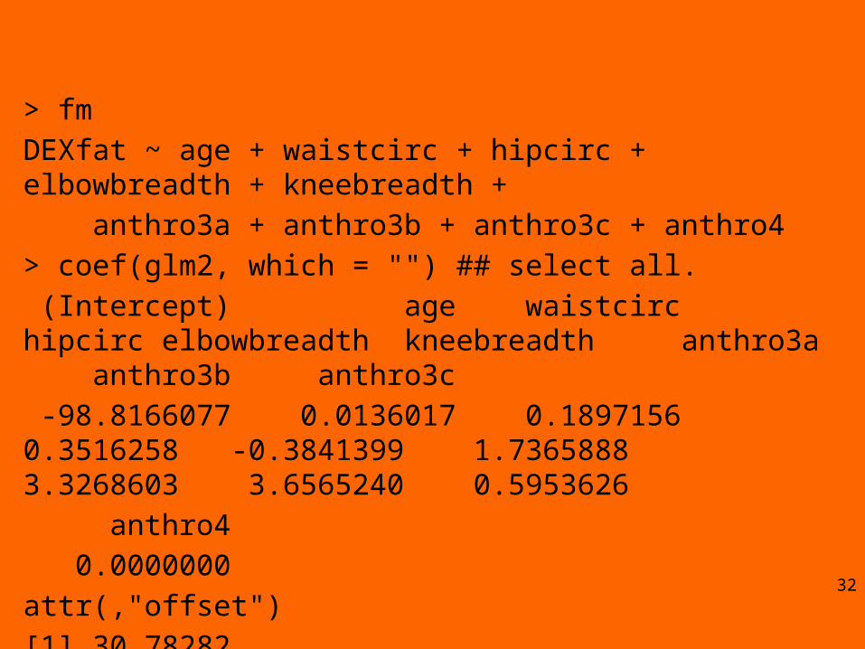
> fm

DEXfat ~ age + waistcirc + hipcirc + elbowbreadth + kneebreadth +

anthro3a + anthro3b + anthro3c + anthro4

> coef(glm2, which = "") ## select all.

(Intercept) age waistcirc hipcirc elbowbreadth kneebreadth anthro3a anthro3b anthro3c

-98.8166077 0.0136017 0.1897156 0.3516258 -0.3841399 1.7365888 3.3268603 3.6565240 0.5953626

anthro4

0.0000000

attr(,"offset")

[1] 30.78282 32

plot(glm2, off2int = TRUE)

33

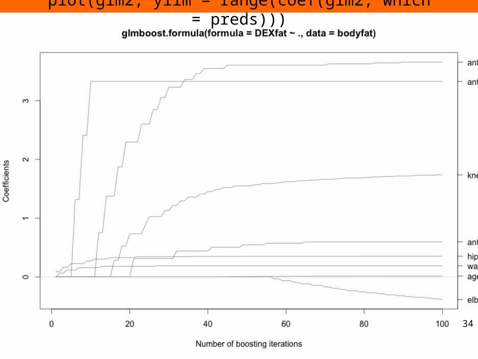
plot(glm2, ylim = range(coef(glm2, which = preds)))

34

> summary(bodyfat)

age DEXfat waistcirc hipcirc elbowbreadth kneebreadth anthro3a

Min. :19.00 Min. :11.21 Min. : 65.00 Min. : 88.00 Min. :5.200 Min. : 7.200 Min. :2.400

1st Qu.:42.00 1st Qu.:22.32 1st Qu.: 78.50 1st Qu.: 96.75 1st Qu.:6.200 1st Qu.: 8.600 1st Qu.:3.540

Median :56.00 Median :29.63 Median : 85.00 Median :103.00 Median :6.500 Median : 9.200 Median :3.970

Mean :50.86 Mean :30.78 Mean : 87.38 Mean :105.28 Mean :6.508 Mean : 9.301 Mean :3.869

3rd Qu.:62.00 3rd Qu.:39.33 3rd Qu.: 99.75 3rd Qu.:111.15 3rd Qu.:6.900 3rd Qu.: 9.800 3rd Qu.:4.155

Max. :67.00 Max. :62.02 Max. :117.00 Max. :132.00 Max. :7.400 Max. :11.800 Max. :4.680

anthro3b anthro3c anthro4

Min. :2.580 Min. :2.050 Min. :3.180

1st Qu.:4.060 1st Qu.:3.480 1st Qu.:5.040

Median :4.390 Median :3.990 Median :5.530

Mean :4.291 Mean :3.886 Mean :5.398

3rd Qu.:4.660 3rd Qu.:4.345 3rd Qu.:5.840

Max. :5.010 Max. :4.620 Max. :6.370

35

Other forms of boosting• Gamboost = Generalized Additive Model -

Gradient boosting for optimizing arbitrary loss functions, where component-wise smoothing procedures are utilized as (univariate) base-learners.

36

> gam1 <- gamboost(DEXfat ~ bbs(hipcirc) + bbs(kneebreadth) + bbs(anthro3a),data = bodyfat)

> #Using plot() on a gamboost object delivers automatically the partial e ects of the di erent base-learners:ff ff> par(mfrow = c(1,3)) ## 3 plots in one device

> plot(gam1) ## get the partial effects

# bbs, bols, btree..

37

38

> gam2 <- gamboost(DEXfat ~ ., baselearner = "bbs", data = bodyfat,control = boost_control(trace = TRUE))

[ 1] .................................................. -- risk: 515.5713

[ 53] ..............................................

Final risk: 460.343

> set.seed(123) ## set seed to make results reproducible

> cvm <- cvrisk(gam2) ## default method is 25-fold bootstrap cross-validation

39

> cvm

Cross-validated Squared Error (Regression)

gamboost(formula = DEXfat ~ ., data = bodyfat, baselearner = "bbs", control = boost_control(trace = TRUE))

1 2 3 4 5 6 7 8 9 10

109.44043 93.90510 80.59096 69.60200 60.13397 52.59479 46.11235 40.80175 36.32637 32.66942

11 12 13 14 15 16 17 18 19 20

29.66258 27.07809 24.99304 23.11263 21.55970 20.40313 19.16541 18.31613 17.59806 16.96801

21 22 23 24 25 26 27 28 29 30

16.48827 16.07595 15.75689 15.47100 15.21898 15.06787 14.96986 14.86724 14.80542 14.74726

31 32 33 34 35 36 37 38 39 40

14.68165 14.68648 14.64315 14.67862 14.68193 14.68394 14.75454 14.80268 14.81760 14.87570

41 42 43 44 45 46 47 48 49 50

14.90511 14.92398 15.00389 15.03604 15.07639 15.10671 15.15364 15.20770 15.23825 15.30189

51 52 53 54 55 56 57 58 59 60

15.31950 15.35630 15.41134 15.46079 15.49545 15.53137 15.57602 15.61894 15.66218 15.71172

61 62 63 64 65 66 67 68 69 70

15.72119 15.75424 15.80828 15.84097 15.89077 15.90547 15.93003 15.95715 15.99073 16.03679

71 72 73 74 75 76 77 78 79 80

16.06174 16.10615 16.12734 16.15830 16.18715 16.22298 16.27167 16.27686 16.30944 16.33804

81 82 83 84 85 86 87 88 89 90

16.36836 16.39441 16.41587 16.43615 16.44862 16.48259 16.51989 16.52985 16.54723 16.58531

91 92 93 94 95 96 97 98 99 100

16.61028 16.61020 16.62380 16.64316 16.64343 16.68386 16.69995 16.73360 16.74944 16.75756

Optimal number of boosting iterations: 33 40

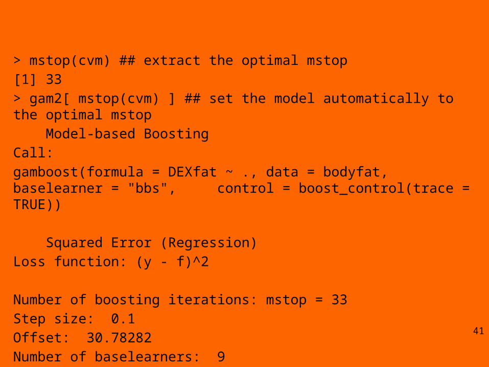
> mstop(cvm) ## extract the optimal mstop

[1] 33

> gam2[ mstop(cvm) ] ## set the model automatically to the optimal mstop

Model-based Boosting

Call:

gamboost(formula = DEXfat ~ ., data = bodyfat, baselearner = "bbs", control = boost_control(trace = TRUE))

Squared Error (Regression)

Loss function: (y - f)^2

Number of boosting iterations: mstop = 33

Step size: 0.1

Offset: 30.78282

Number of baselearners: 9 41

plot(cvm)

42

> names(coef(gam2)) ## displays the selected base-learners at iteration 30

[1] "bbs(waistcirc, df = dfbase)" "bbs(hipcirc, df = dfbase)" "bbs(kneebreadth, df = dfbase)"

[4] "bbs(anthro3a, df = dfbase)" "bbs(anthro3b, df = dfbase)" "bbs(anthro3c, df = dfbase)"

[7] "bbs(anthro4, df = dfbase)"

> gam2[1000, return = FALSE] # return = FALSE just supresses "print(gam2)"

[ 101] .................................................. -- risk: 423.9261

[ 153] .................................................. -- risk: 397.4189

[ 205] .................................................. -- risk: 377.0872

[ 257] .................................................. -- risk: 360.7946

[ 309] .................................................. -- risk: 347.4504

[ 361] .................................................. -- risk: 336.1172

[ 413] .................................................. -- risk: 326.277

[ 465] .................................................. -- risk: 317.6053

[ 517] .................................................. -- risk: 309.9062

[ 569] .................................................. -- risk: 302.9771

[ 621] .................................................. -- risk: 296.717

[ 673] .................................................. -- risk: 290.9664

[ 725] .................................................. -- risk: 285.683

[ 777] .................................................. -- risk: 280.8266

[ 829] .................................................. -- risk: 276.3009

[ 881] .................................................. -- risk: 272.0859

[ 933] .................................................. -- risk: 268.1369

[ 985] ..............

Final risk: 266.9768 43

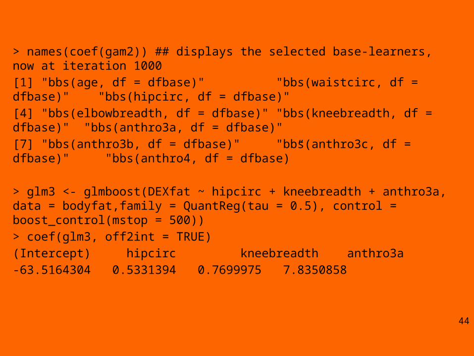
> names(coef(gam2)) ## displays the selected base-learners, now at iteration 1000

[1] "bbs(age, df = dfbase)" "bbs(waistcirc, df = dfbase)" "bbs(hipcirc, df = dfbase)"

[4] "bbs(elbowbreadth, df = dfbase)" "bbs(kneebreadth, df = dfbase)" "bbs(anthro3a, df = dfbase)"

[7] "bbs(anthro3b, df = dfbase)" "bbs(anthro3c, df = dfbase)" "bbs(anthro4, df = dfbase)”

> glm3 <- glmboost(DEXfat ~ hipcirc + kneebreadth + anthro3a, data = bodyfat,family = QuantReg(tau = 0.5), control = boost_control(mstop = 500))

> coef(glm3, off2int = TRUE)

(Intercept) hipcirc kneebreadth anthro3a

-63.5164304 0.5331394 0.7699975 7.8350858

44

45

Compare to rpart> fattree<-rpart(DEXfat ~ ., data=bodyfat)

> plot(fattree)

> text(fattree)

> labels(fattree)

[1] "root" "waistcirc< 88.4" "anthro3c< 3.42" "anthro3c>=3.42" "hipcirc< 101.3" "hipcirc>=101.3"

[7] "waistcirc>=88.4" "hipcirc< 109.9" "hipcirc>=109.9"

46

47

cars

48

iris

49

cars

50

51

OptimizingCoefficients:

(Intercept) speed

-60.331204 3.918359

attr(,"offset")

[1] 42.98

Call:

glmboost.formula(formula = dist ~ speed, data = cars, control = boost_control(mstop = 1000), family = Laplace())

Coefficients:

(Intercept) speed

-47.631025 3.402015

attr(,"offset")

[1] 35.9999952

53

Sparse matrix example> coef(mod, which = which(beta > 0))

V306 V1052 V1090 V3501 V4808 V5473 V7929 V8333 V8799 V9191

2.1657532 0.0000000 4.8756163 4.7068006 0.4429911 5.4029763 3.6435648 0.0000000 3.7843504 0.4038770

attr(,"offset")

[1] 2.90198

54

55

Aside: Boosting and SVM…• Remember “margins” from the SVM?

Partitioning the “linear” or transformed space?

• In boosting we are effectively (not explicitly) attempting to maximize the minimum margin of any training example

56

Variants on boosting – loss fncars.gb <- blackboost(dist ~ speed, data = cars, control = boost_control(mstop = 50))

### plot fit

plot(dist ~ speed, data = cars)

lines(cars$speed, predict(cars.gb), col = "red")

57

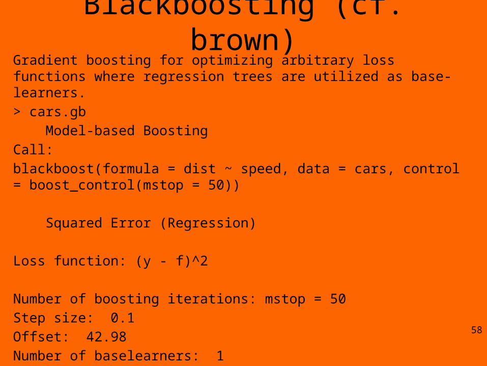
Blackboosting (cf. brown)Gradient boosting for optimizing arbitrary loss functions where regression trees are utilized as base-learners.

> cars.gb

Model-based Boosting

Call:

blackboost(formula = dist ~ speed, data = cars, control = boost_control(mstop = 50))

Squared Error (Regression)

Loss function: (y - f)^2

Number of boosting iterations: mstop = 50

Step size: 0.1

Offset: 42.98

Number of baselearners: 1 58