1 Planetary Masses and Orbital Parameters from Radial … · 2007-10-30 · ences between Keplerian ﬁts, ... 2 1 Planetary Masses and Orbital Parameters from Radial Velocity Measurements

Extrasolar Planets: Formation, Detection and Dynamics. Edited by Rudolf DvorakCopyright © 2007 WILEY-VCH Verlag GmbH & Co. KGaA, WeinheimISBN: 978-3-527-40671-5

1

1Planetary Masses and Orbital Parameters fromRadial Velocity MeasurementsC. Beaugé, S. Ferraz-Mello, and T. A. Michtchenko

Abstract

So far practically all detections of extrasolar planets have been obtained fromradial velocity data, in which the presence of planetary bodies is deduced fromtemporal variations in the radial motion of the host star. To perform any dy-namical study for these systems, it is necessary to specify: (i) initial condi-tions (mass and orbital elements) and (ii) an adequate coordinate system fromwhich to construct the equations of motion. This chapter discusses both ofthese points.

In the first part we introduce the reader to the process of orbital determi-nation from Doppler data, for both single and multiple exoplanetary systems.We distinguish between primary parameters (which are obtainable directlyfrom the observational data) and secondary parameters which require addi-tional information about the system, such as the stellar mass or inclination ofthe orbital plane. For multiple planetary systems we also discuss the differ-ences between Keplerian fits, in which the mutual perturbations between theplanets are neglected, and dynamical (or N-body) fits.

The second part of the chapter is devoted to the construction of the equa-tions of motion in different coordinate systems. Special attention is given tothe Hamiltonian formalism in barycentric, Jacobi and Poincaré coordinates,and we explain how to obtain orbital elements in each case. Finally, we dis-cuss some of their advantages and disadvantages, particularly with respect toorbital fits and general dynamical studies.

1.1Exoplanet Detection

Planets are very dim objects, and their direct observation is an extremely dif-ficult task. Even Jupiter, the biggest planet in our own solar system, has onlyabout 10−9 times the luminosity of the sun, making a similar exoplanet un-observable to us by present techniques. The first direct observation of an ex-

2 1 Planetary Masses and Orbital Parameters from Radial Velocity Measurements

oplanet (GQ Lupi) only occurred in 2005 with VLT and, as of July 2006, threeother exoplanets have also been imaged (2M1207, AB Pic and SCR 1845). How-ever, most of the exoplanetary bodies have never been seen at all.

If an exoplanet cannot be seen, how can we know it is there? The basic ideais that, even if invisible, the presence of a planetary body may affect the lumi-nosity of the star, or its motion with respect to background objects. Thus, wemay deduce the existence of a planet by analyzing changes in some observableaspect of the star it revolves around. Such ”indirect” detection methods arethe main backbone in current discovery strategies of exoplanets. Five differ-ent techniques have been proposed and developed in recent years: (i) StellarTransit, (ii) Radial Velocity Curves (Doppler), (iii) Gravitational Micro-lensing,(iv) Stellar Interferometry and (v) Astrometry. For details on these and otherproposed methods, the reader is referred to Perryman [1] for a very compre-hensive review.

Although very promising, Micro-lensing and Astrometry are still far fromfulfilling their potential. Only four planetary candidates have been proposedbased on micro-lensing techniques (OGLE-05-071L, OGLE-05-169L, OGLE-05-390L and OGLE235-MOA53), and even though some estimate may be obtainedconcerning mass and orbital period, there is no information about the remain-ing orbital elements. A similar picture can be given for interferometric tech-niques, and at present only four positive detections are counted. Astrometryhas yet to yield a discovery, although the projected launch of several spacetelescopes (e.g., Kepler, TPF) will almost certainly change this picture. Conse-quently, and at least at present, practically all the currently exoplanet popula-tion has been obtained either by Stellar Transit or Doppler. The former is thesubject of another chapter of this book, while the latter is the main objective ofthe present text.

1.2Radial Velocity in Astrocentric Elements

The observation of a Doppler shift of the spectral lines of a star denounces achange in the velocity of the star with respect to the observer. Since the ob-server himself is moving with a velocity ∼ 30 km s−1, variable in direction, itis necessary to subtract this motion from the observational data and reduce itto the barycenter of the solar system (for a description of the necessary opera-tions see Ferraz-Mello et al. [2]).

The velocity of an isolated star, with respect to the barycenter of the solarsystem, is constant, at least for times short as compared to the timescale ofgalactic motion. However, if it has N planetary companions, the star willdisplay a motion around the common barycenter of the system (see Fig. 1.1).

1.2 Radial Velocity in Astrocentric Elements 3

Fig. 1.1 The sinusoidal motion of a star due to the presence of aplanetary companion. The faint field stars are used as a referenceframe.

In order to understand this effect, we begin studying the kinematics of a singleplanet in elliptic orbit around the star. In an astrocentric reference frame, theposition and velocity vectors of the planet are given by Brouwer and Clemence[3] and Murray and Dermott [4]:

r = r cos f ı + r sin f j (1.1)

v = − 2πa

T√

1 − e2

[sin f ı − (e + cos f ) j

]

where

r =a(1 − e2)

1 + e cos fd fdt

=2πa2

Tr2

√1 − e2 (1.2)

Here r is the magnitude of the radius vector r, the velocity vector is denoted byv, f is the true anomaly, a is the astrocentric semi-major axis, e is the eccentric-ity, and ı and j are two unit vectors in the orbital plane. The first is orientatedin the direction of the pericenter, and the latter is orthogonal to it. The orbitalperiod T can be obtained directly from Kepler’s third law. Denoting by m0 themass of the star and m the mass of the planet, we have:

n2a3 = G(m0 + m) (1.3)

where the mean motion n = 2π/T is the mean angular velocity along theorbit.

We must now transform these vectors to a new coordinate system that isindependent of the plane of orbital motion. For exoplanets it is customary touse a modification of the so-called Herschel astrocentric coordinates, whichwere first developed for studies of visual double stars. It uses the sky (i.e., a


plane tangent to the celestial sphere) as the reference plane, and a schematicview is presented in Fig. 1.2. The x-axis is taken along the intersection linebetween the orbital plane and the sky. Its direction is chosen towards γ, whichis the node where the motion of the planet is directed towards the observer.The y-axis is also tangent to the celestial sphere, and is such that the resultingsystem is right-handed. Finally, the z-axis is directed along the line of sight,away from the observer.

Fig. 1.2 The rotated astrocentric reference frame showing theorbital plane and the plane tangent to the celestial sphere (sky).The origin of the angles is the point γ.

In this coordinate system, the unit vectors ı, j and k of the orbital plane havecomponents:

ı =

⎛⎝ cos ω

sin ω cos I− sin ω sin I

⎞⎠ j =

⎛⎝ − sin ω

cos ω cos I− cos ω sin I

⎞⎠ k =

⎛⎝ 0

sin Icos I

⎞⎠ (1.4)

k is perpendicular to the orbital plane of the planet. This decomposition of theunit vectors is analogous to the transformations commonly used in celestialmechanics to pass to coordinates with respect to the ecliptic (except that herewe fix Ω = π). I is the inclination of the orbital plane with respect to the sky,and the argument of the pericenter is given by ω + π. The addition of theangle π is due to the direction of the x-axis, which is chosen opposite to the“ascending node” N.


We can now obtain the components of r and v in this new reference frame.After a few simple algebraic manipulations, we obtain the velocity v =(vx, vy, vz) where:

vx = − 2πa

T√

1 − e2

[sin ( f + ω) + e sin ω

]

vy =2πa cos I

T√

1 − e2

[cos ( f + ω) + e cos ω

](1.5)

vz = − 2πa sin I

T√

1 − e2


]

Having the astrocentric velocity vector of the planet in the desired referenceframe, we can pass to barycentric coordinates. Calling V the barycentric ve-locity vector of the planet, and V∗ that of the star, we have that v = V − V∗.On the other hand, since the barycenter is fixed in this reference frame, wehave m0V∗ + mV = 0. Solving for V∗, we obtain:

V∗ = − mm0 + m

v (1.6)

which represents the velocity of the motion of the star around the center ofmass of the system. To calculate the velocity actually detected by the ob-server, we must add the velocity V0 of the barycenter itself with respect tobackground stars.

It is useful to decompose this observable velocity into the tangential velocitycomponent Vt and the radial velocity Vr = V∗z + V0z. The former causes adisplacement of the position of the star with respect to background stars. Itsmeasurement is the role of astrometry but, as mentioned before, telescopes onearth are currently not able to detect these variations except in a few cases. Theradial velocity Vr is far easier to detect, even with ground-based instruments,due to changes in the frequency (Doppler shift) of spectral lines from the star’sspectrum. The best stellar candidates are those that, on one hand, contain afair amount of absorption lines in the visible spectrum (i.e., must not be toohot) but, on the other hand, the number of lines must not be too large (i.e.,the star must not be too cold). Thus, the best candidates are stars of spectraltype F or G; in other words, similar to our own sun. A complete expressionfor the radial velocity can be found simply by substituting V∗z from Eqs. (1.5)and (1.6), and yields:

Vr =2πa

T√

1 − e2

m sin I(m + m0)


]+ Vr0 (1.7)

where Vr0 = V0z is the (constant) reference radial velocity of the barycenter.


The extension to N planets is straightforward and follows the same lines, aslong as we neglect mutual perturbations and assume Keplerian solutions. Wecan then write the complete radial velocity of the star at a given time t as:

Vr(t) =N

∑i=1

Ki

[cos ( fi + ωi) + ei cos ωi

]+ Vr0 (1.8)

where

Ki =mi sin Ii

M2πai

Ti

√1 − e2

i

(1.9)

and

M =N

∑i=0

mi (1.10)

is the total mass of the system (star and planets). Transforming from semi-major axis to mean motions via Kepler’s third law, we can then rewrite thecoefficients Ki as:

Ki =(G(M + mi)

)1/3 mi sin Ii

M n1/3i (1 − e2

i )−1/2 (1.11)

or, more succinctly, as

Ki = Fi(M, mi, Ii) n1/3i (1 − e2

i )−1/2 (1.12)

where Fi(M, mi, Ii) is sometimes called the ”mass function” and groups allthe terms that depend explicitly on the stellar and planetary masses, as wellas the orbital inclination. This expression is valid only for astrocentric or-bital elements. If Jacobian coordinates are employed, the expression given byEq. (1.38) must be used.

The basis of the Doppler method is then to build an observational data baseof the changes in the radial velocity of a target star. These radial velocity datapoints represent a discretized representation of the radial component of theleft-hand side of Eq. (1.8). The idea now is to deduce, from this data set, themasses and orbital parameters of all the planetary companions that make upthe right-hand member of the same equation.

Note that Vr(t) is the sum of N periodic terms, each with semi-amplitudeKi. However, the true anomaly fi is only a linear function of time in the caseof circular orbits ei = 0. In the general elliptic case, only the mean anomaly�i has a constant derivative (given by the mean motion ni). The relationshipbetween f and � is given in terms of the (intermediate) eccentric anomaly u,


and via the following two equations:

tan ( f /2) =√

1 + e1 − e

tan (u/2) (1.13)

u − e sin u = � = n(t − τ)

The second expression is the classical Kepler equation, and must be solvediteratively to obtain the passage from � (or the time) to the eccentric anomaly.The quantity τ is sometimes referred to as the time of passage through thepericenter. Finally, the mean motion n is related to the semi-major axis andmasses through Kepler’s third law.

As an example, Fig. 1.3 shows the shape of two fictitious radial velocitycurves, constructed from Eq. (1.8) with only one planet. The continuous lineshows the case of a circular orbit (e = 0), while the dashed line presents anexample of a highly elliptic body (e = 0.6). Although both periods and semi-amplitudes are the same, the second curve shows distinctive peaks each timethe planet crosses the pericenter of its orbital motion. Another noticeable effectof the eccentricity is a change in the averaged value of Vr. Once again, this isdue to the nonlinear behavior of the true anomaly f for noncircular orbits.

0 20 40 60 80 100time

-1.5

-1

-0.5

0

0.5

1

1.5

2

Vr

e=0

e=0.6

Fig. 1.3 Fictitious radial velocity curves, using Eq. (1.8) withK = 1, ω = 180 degrees and T = 50 in arbitrary time units.Continuous line corresponds to a circular orbit, while the dashedcurve was calculated with e = 0.6.

As a final important point, it must be stressed that there is no free angleequivalent to the longitude of the ascending node Ω that can be simply addedto the orbital elements of the planets. As shown in Fig. 1.2, Ω measures the an-gular distance from the x-axis and the “ascending node” N, and in Herschel’s


modified coordinate system it is set to Ω = π. Expressions (1.5) for the veloc-ity components (vx, vy, vz) were derived for this orientation of the x-axis, andthus implicitly depend on this choice of Ω. Any other value for Ω would beinconsistent with the orbit issued from the observations.

1.3Orbital Fits from Radial Velocity Curves

1.3.1Primary Parameters

Until recently, radial velocity data were zealously guarded by the observa-tional teams and not available to the general scientific community. Fortu-nately this picture is changing (albeit slowly), and some information is cur-rently available from the on-line versions of the published papers. This infor-mation is already pre-processed, in the sense that all the necessary steps havebeen taken to reduce the velocities to the barycenter of our solar system.

A real example of a radial velocity data set can be seen in Fig. 1.4 (sym-bols). Each point corresponds to discrete values Vr(tk) of HD 82943, a systemknown to contain two planets in a 2/1 mean-motion resonance (see Mayor etal. [5], Ferraz-Mello et al. [6]). Doppler data is usually presented in a multi-column format giving, among other information, the times of observation tk(usually in Julian days), radial velocities Vrk = Vr(tk) (usually in meters persecond) and the expected uncertainties εk (also in m s−1). This latter valuescorrespond to the size of the error bar of the radial velocity data, and a Gauss-ian error distribution is usually assumed. Current instrumentation and re-duction techniques have lowered the values of εk to the order of a few m s−1.When observations include data from more than one instrument, the origin ofeach data segment is also included in the files.

With the numerical data in hand, we first assume that the temporal varia-tions of Vr are caused by the presence of one (or more) exoplanets, and there-fore correspond to time-discrete values of a function of type (1.8). That beingthe case, our second task is to develop a numerical algorithm to deduce thenumber of periodic terms contained in the signal (i.e., number of planets N),and for each to estimate the values of the set

(Ki, ni, ei, ωi, τi) (i = 1, . . . , N) (1.14)

plus the barycentric radial velocity Vr0. These are sometimes referred to asthe “primary parameters” of an orbital fit. The individual planetary masses(multiplied by sin Ii) are derived from the calculated value of Ki and the massfunction. Notice that the number of free parameters is equal to 5N + 1, con-sisting of five orbital parameters per planet plus the radial velocity Vr0 of the

1.3 Orbital Fits from Radial Velocity Curves 9

(a)

(b)

8000

8050

8100

8150

8200

8250

Vr [

m/s

]

51500 52000 52500

51500 52000 52500time (JD-240000) [days]

-20

-10

0

10

20

o-c

[m

/s]

Fig. 1.4 (a) Radial velocity data points of the HD82943 star,together with an orbital with two planets. (b) Residuals from thefit. Figure obtained with a dynamical two-planet fit.

barycenter of the extrasolar system. As we shall show later on, Vr0 does notnecessarily correspond to the time-averaged value of Vr, unless all exoplan-ets move in circular orbits. In the case where the data includes values fromdifferent instruments and observatories, individual values of Vr0 are usuallyassigned. As a final note of caution, in the case of more than one planet, thecalculated orbital periods (or mean motions) are not osculating, but apparent(see [6]).

The mass of the star is taken from sophisticated stellar models. However,one must keep in mind that, even for Hipparcos stars having the best availablespectroscopy and astrometry, the more accurate models do not allow to knowthe masses better than � 8 percent (Allende et al. [7]). This fact supersedessome discussions on the nature of the published planetary elements, if astro-centric or barycentric. The difference between coordinates in these systemsis usually much smaller than the uncertainty in our knowledge of the stellarmass.

Even though the functional form of Vr(t) given by (1.8) is the sum of peri-odic terms, it is not usually convenient to attempt an orbital fit using a direct


Fourier analysis. The reasons are twofold. First, a precise identification ofthe leading frequencies with Fourier decomposition requires that the obser-vational data should cover several periods. This is not usually the case, spe-cially for planets with large semi-major axis. Second, radial velocity data is notevenly spaced in the time axis and, even worse, usually contains months-longgaps where observations are not favorable. Both problems can be overcomeusing a more general Fourier method, such as the Dates Compensated FourierTransform [8] or the CLEANest algorithm [9], which were specifically devel-oped for nonequidistant data points and arbitrary frequencies. However, aleast-squares algorithm is usually more precise and requires less fine-tuningof the results. Thus, practically all orbital fits have been calculated using thisapproach.

We then search for adequate coefficients (1.14) of a fitting function y(t), oftype (1.8), such that the residual function

Q2 = ∑tn

[y(tn) − Vr(tn)]2

ε2n

(1.15)

is minimum. Notice that this definition includes the uncertainty of each datapoint Vr(tn) and has the advantage of considering different precisions amongthe data. This is particularly important when mixing observations from differ-ent instruments. In the case where the εn correspond to the standard deviationof the data, Q2 is equal to the χ2 of the data modelization.

Initially, deterministic versions of nonlinear least-squares were used, suchas hill-climbing techniques or the Levenberg–Marquardt method (see [5, 10,11]). The main drawback with these methods is that they are unable to dis-tinguish between local and global minima of Q2; consequently, there is noguarantee that the calculated orbital elements correspond to the best fit ofthe data sets. Since the number of free parameters can be large, the shapeof the residual function may be complex and contain numerous local minima,several of them possibly with similar values. Moreover, since the problem ishighly nonlinear, the result may be highly sensitive to the initial values of theparameters. An example of this behavior was given by Mayor et al. [5] for thetwo HD 82943 planets. The authors presented two different fits: in the first theorbital eccentricities of the planets were (e1, e2) = (0.4, 0.0) and for the second(e1, e2) = (0.4, 0.18). Although the eccentricity of the outer planet changedsignificantly, the value of Q2 only varied by � 0.1 percent. What is moreworrisome in this case is that the best-fit solutions found by several authorsactually corresponds to orbits which are dynamically unstable in timescales ofthe order of 105–106 years (see [6]). Thus, given a limited set of observations,the orbital configuration of the real planets does not necessarily correspond tothe best fit.


Since results of orbital fits sometimes seem very sensitive to the numericalmethod and/or data set, we need to fine-tune our techniques. We need a strat-egy (or method) that can identify the global extrema of the residual function.Additionally, we must be able to estimate the confidence levels (i.e., errors)in the orbital parameters themselves. Due to the highly nonlinear character-istics of the equations, it is not correct to assume Gaussian distribution errorsin (V0r,Ki, ni, ei, ωi, τi). Consequently, the standard deviations that are some-times seen, alongside the best fits, can be misleading and must be consideredwith utmost care [12].

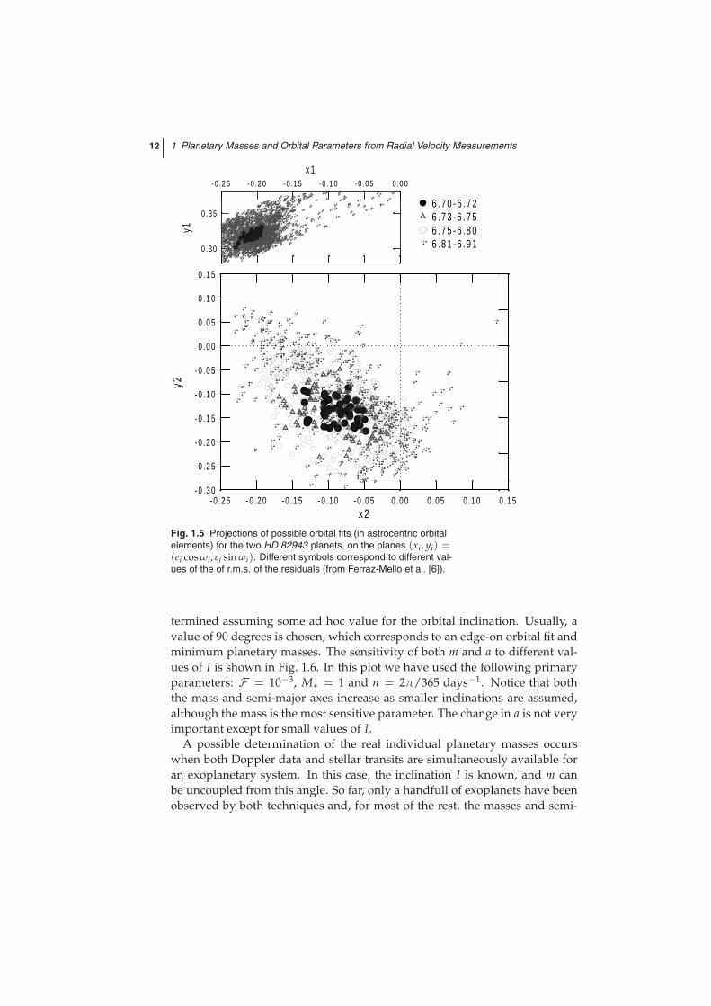
Considering that the result of classical nonlinear best-fit methods dependson the initial guess, a possible approach towards a global minimum is to ap-ply the same method to a large number of initial conditions, distributed ran-domly in the parameter space. This so-called Monte Carlo approach was usedby Brown [13] to the Vr data from HD 72659. A year later, Ferraz-Mello et al.[6] employed a similar approach to study the two-planet system of HD 82943.One of the main advantages of this type of Monte Carlo algorithm is the pos-sibility of estimating the confidence region of each of the orbital elements; inother words, the different possible primary parameters that are all compati-ble with the given data set. For the particular case of HD 82943, we found alarge set of different orbital fits which yield practically the same value of theresidual function (see Fig. 1.5). Thus, in some cases, it is not possible to give asingle value of the parameter set as the “correct” orbital fit.

A different strategy for the search of global minima of the orbital fit, is theuse of genetic algorithms. This technique is based on natural selection (mim-icking the behavior of biological populations), by which an initially randompopulation of initial guesses evolves towards the global minimum. Althoughthis approach can require larger computational resources than deterministicmethods, it has proved to be extremely robust in all applications to exoplan-etary systems (e.g. [14, 15]). Other advantages of this approach include itssimple manipulation, and its ability to introduce non-Gaussian error estima-tions with no significant complications. A recommended introductory text ongenetic algorithms can be found in Charbonneau [16].

1.3.2Secondary Parameters

Whatever the chosen numerical approach, the orbital fit yields values forV0r,Ki, ni, ei, ωi and τi. From these we must now estimate the planetarymasses and semi-major axes. These quantities are related to the primary pa-rameters through the Eqs. (1.3) and (1.11). Notice that we have two algebraicequations with three unknowns, and it is impossible to separate the valueof sin Ii from the planetary mass. Thus, the values of m and a must be de-


- 0 .2 5 -0 .2 0 -0 .1 5 -0 .1 0 -0 .0 5 0 .0 0 0 .0 5 0 .1 0 0 .1 5x 2

-0 .3 0

-0 .2 5

-0 .2 0

-0 .1 5

-0 .1 0

-0 .0 5

0 .0 0

0 .0 5

0 .1 0

0 .1 5

y2

6 .7 0 - 6 .7 26 .7 3 - 6 .7 56 .7 5 - 6 .8 06 .8 1 - 6 .9 10 .30

0 .35

y1- 0 .2 5 -0 .2 0 -0 .15 -0 .10 -0 .05 0 .0 0

x 1

Fig. 1.5 Projections of possible orbital fits (in astrocentric orbitalelements) for the two HD 82943 planets, on the planes (xi, yi) =(ei cos ωi, ei sin ωi). Different symbols correspond to different val-ues of the of r.m.s. of the residuals (from Ferraz-Mello et al. [6]).

termined assuming some ad hoc value for the orbital inclination. Usually, avalue of 90 degrees is chosen, which corresponds to an edge-on orbital fit andminimum planetary masses. The sensitivity of both m and a to different val-ues of I is shown in Fig. 1.6. In this plot we have used the following primaryparameters: F = 10−3, M∗ = 1 and n = 2π/365 days−1. Notice that boththe mass and semi-major axes increase as smaller inclinations are assumed,although the mass is the most sensitive parameter. The change in a is not veryimportant except for small values of I.

A possible determination of the real individual planetary masses occurswhen both Doppler data and stellar transits are simultaneously available foran exoplanetary system. In this case, the inclination I is known, and m canbe uncoupled from this angle. So far, only a handfull of exoplanets have beenobserved by both techniques and, for most of the rest, the masses and semi-


0 15 30 45 60 75 90inclination [deg]

0

1

2

3

planetary mass

semimajor axis

Fig. 1.6 Variation of the planetary mass m (in units of stel-lar mass) and semi-major axis a (in AU), as a function of theunknown inclination of the orbital plane I, for fixed values of theprimary parameters of an orbital fit. The plot was constructed withF = 10−3, M∗ = 1 and n = 2π/365 days−1.

major axis are still affected by Ii. At first hand, this seems a major limitation forany dynamical analysis, since these are probably the most important param-eters. However, if for multiple planetary systems we assume that all planetsare co-planar, then the ratios:

mj

mi

aj

ai(i, j = 1, . . . , N) (1.16)

are unaffected by the value of the spatial inclination. In other words, althoughthe individual values of mi and ai may be unknown, the relative values can bededuced, and used in our dynamical studies.

1.3.3N-Body Fits

In the previous analysis, we have assumed that the motion of each planetorbiting a given star can be modeled by a Keplerian ellipse. This is an approx-imation since mutual perturbations will cause the orbital elements to changewith time. If the estimated values for the planetary masses (minimum values)are sufficiently small or the mutual separation (i.e., ai/aj) are sufficiently large,we can assume that the orbital variations are negligible within the timespanof the observations. In that case, the multi-Keplerian fits presented before are


valid approximations to the problem. However, if the mutual perturbationsare large, we must modify the orbital fit to accommodate nonconstant orbitalelements. This is usually referred to dynamical (or N-Body) orbital fits.

We assume a data file consisting of several observations, starting at time t =t0 and ending at t = tM. In this interval, the orbital elements are allowed tovary with time. A dynamical fit proceeds the same way as the multi-Keplerianversion, except for the calculation of the model values of Vr(ti). For perturbedorbits, it is no longer optimal to use (1.8) to relate the radial velocity with theorbital elements. The procedure can be separated into the following steps:

1. Specify initial conditions (ni0, ei0, ωi0, τi0, Ii0) for all the planets, which willcorrespond to the astrocentric orbits at the beginning of the observations.The orbital period of each planet must be osculating, and not apparent [6].We will also require values for the real planetary masses, unaffected by theinclinations Ii.

2. Transform the orbital elements to Cartesian coordinates and velocities. Wewill need Kepler’s third law to obtain the semi-major axes, and thus theresult will depend on the stellar mass m0. From this data we can calculatethe velocity vector of the star V (with respect to the barycenter of the sys-tem) at t0. Choosing the reference frame of the coordinate system tangentto the celestial sphere, the first model value of Vr(t0) will be given by thez-component of V.

3. Using an N-body numerical integrator, calculate the positions of the planetsat all the subsequent times of observation (i.e., t = t1, . . . , tM).

4. For each ti, repeat the calculations in Step 2, and obtain the complete set ofradial velocities Vr(ti).

Having all the values of Vr(ti) for the chosen initial conditions and real plan-etary masses, we can calculate the residual function. The best fit will thenbe the set of initial parameters (ni0, ei0, ωi0, τi0, Ii0) and planetary masses thatminimizes Q2. The use of numerical integrations will obviously increase theamount of CPU time; thus N-body fits are sometimes done as a second-orderapproximation from initial Keplerian parameters.

A factor to be taken into account is the uncertainty in the value of the stellarmass, and its propagation to other quantities in the orbital fit. To obtain ai wemust use Kepler’s third law, and the results depend explicitly on the choiceof m0. A possible way to avoid these problems is to use an adimensional for-mulation for the equations of motion (see [2]). Even if this approach is notemployed, it can easily be seen that the ratios mi/mj and ai/aj between anytwo planets are unaffected by the particular value of m0. The same character-istic was also seen in the dependence of the orbital fits with the inclinations I.


Thus, any dynamical study that can be constructed as a function of these ratioswill yield results virtually independent of I and m0.

One of the most important traits of dynamical fits is its theoretical ability toassess the planetary masses independently of other detection methods, thusallowing us to bypass the limitations of radial velocity data. However, thistask is not always possible. Even for fixed edge-on systems, the differencebetween a dynamical and a multi-Keplerian fit is appreciable only if: (i) theplanets are under significant mutual perturbations and, (ii) the observationaltimespan is large. This is true only in a very few cases, the most well knownexample being GJ 876 [10]. For almost all other known planetary systems, thedistinction is practically unnoticeable.

An example is given in Fig. 1.7 for the HD 82943 planets. We can see littledifference between both fits (Keplerian and dynamical) within the observa-tion interval and, at least for this system, both models yield similar results.However, the divergence between results will increase with time, and longerobservational timespans should be able to detect the effects of mutual pertur-bations between the planets.

2 0 0 0 .0 2 00 2.0 2 0 0 4 .0 2 0 0 6 .0 2 0 0 8 .0T I ME (yr )

-1 5 0

-1 0 0

-5 0

0

5 0

1 0 0

Radi

al V

eloc

ity (

m/s

)

Fig. 1.7 Reconstruction of the radial velocity curve for HD 82943,from a multi-Keplerian fit (gray dots) and an N-body fit (blackdots). The solid line shows the difference (Keplerian minus dy-namical). For more details, see Ferraz-Mello et al. [6].

Since dynamical fits are not necessary for most planetary systems, in prac-tice we are still not able to decouple the planetary masses from the inclina-tions. The values of Ii are not usually considered variables, but fixed at some


initial value, and co-planarity between the planets is assumed. Thus, the truepotential of N-body fits is still far from being fulfilled. Once again, however,larger observational timespans will certainly change this picture.

1.4Coordinate Systems and Equations of Motion

Even with all the limitations and uncertainties, stemming both from the ob-servations and reduction techniques, orbital fits yield (minimum) masses andorbital elements of the planets in a given stellar system. As a first step towardsa dynamical study, we must construct their equations of motion.

Suppose a system consisted of a star of mass m0 and N planets of massmi, thus making this a (N + 1)-body problem. Let Xi denote the positionvectors of all bodies with respect to an inertial reference frame centered in thebarycenter of the system. Then, from Newton’s law of gravitation, we have:

Xi = −GM

∑j = 0j �= i

mjXi − Xj

|Xi − Xj|3 (1.17)

where the double dot denotes the second derivative with respect to the time.Introducing the astrocentric positions of the planets as ri = Xi − X0, we canwrite the equations of motion for the planets in astrocentric variables as:

ri = −G (m0 + mi)|ri|3 ri + G

M

∑j = 1j �= i

mj

(rj − ri

|rj − ri|3 − rj

|rj|3)

(1.18)

In terms of these coordinates, the barycentric motion of the star is given by:

X0 = −∑Ni1

miri

∑Ni1

mi(1.19)

The second term inside the brackets is due to the noninertiality of the astro-centric reference frame, and is caused by the perturbations of the planets onthe motion of the star.

1.4.1Barycentric Hamiltonian Equations

Since dynamical studies of extrasolar planets benefit from the Hamiltonianstructure of the equations of motion, we devote the rest of this section to

1.4 Coordinate Systems and Equations of Motion 17

presenting three different forms of canonical variables and Hamiltonian func-tions. Although this is a well established problem in celestial mechanics, thevast majority of papers deal with the so-called restricted problem in whichonly two bodies have finite masses.

The barycentric Hamiltonian equations of the (N + 1)-body problem areeasy to obtain from Eq. (1.17). Defining Πi = miXi as the linear momentaassociated to each position vector Xi, these variables are canonical, and theHamiltonian of the system is the sum of their kinetic and potential energies:

H =12

N

∑k=0

Π2k

mk− G

N

∑k=0

N

∑j=k+1

mkmj

Δkj(1.20)

where Δkj = |Xk − Xj|. This system has, however, 3(N + 1) degrees of free-dom, that is, six equations more than the usual Laplace–Lagrange formulationof the heliocentric equations of motion.

The system can be reduced to 3N degrees of freedom through the conve-nient use of the trivial conservation laws concerning the inertial motion of thebarycenter. There are two sets of variables used to reduce to 3N the num-ber of degrees of freedom of the above system. Each will be discussed in thefollowing subsections.

1.4.2Jacobi Hamiltonian Formalism

The most popular reduction, due to Jacobi, is widely used in the study of thegeneral three-body problem and of planetary and stellar systems. In Jacobi’sformulation, the position and velocity of the planet m1 are given in a referenceframe with origin in m0 (equal to the star); the position and velocity of m2 aregiven in a reference frame with the origin at the barycenter of m0 and m1; theposition and velocity of m3 are given in a reference frame with the origin at thebarycenter of m0, m1 and m2, and so on. If we denote with ρk (k = 1, . . . , N)the vectors thus defined, we have

ρk = Xk − 1σk

k

∑j=0

mjXj (k = 1, . . . , N) (1.21)

where

σk =k

∑j=0

mj (1.22)

The quantities ρk are our new coordinates; we must now search for theircanonical momenta πk. These can be obtained from the original pk by means


of the simple canonical condition ∑Ni=1(πidρi − ΠidXi) = 0, and give the im-

plicit relation:

Πk = πk −N

∑j=k+1

mkπj

σj−1(1.23)

The reader is referred to Ferraz-Mello et al. [2] for details of this construction.A lengthy, but simple calculation shows that nonconstant terms of the totalkinetic energy, in these variables, are given by

T =N

∑i=1

π2i

2βi(1.24)

where βi are the so-called reduced masses of the Jacobian formulation, definedby

βi =miσi−1

σi(1.25)

The complete Hamiltonian of the relative motion of the N planets, can be writ-ten as:

H = H0 + H1 (1.26)

where:

H0 =N

∑k=1

(π2

k

2βk− Gσk βk

ρk

)(1.27)

H1 = −GN

∑k=1

N

∑j=k+1

mkmj

Δkj− G

N

∑k=1

mk

(m0

Δ0k− σk−1

ρk

)

Constant terms were discarded, since they do not contribute to the equations.This function defines a system with 3N degrees of freedom in the canonicalvariables (ρk, πk) with (k = 1, . . . , N).

Notice that H0 may be written as the sum of N terms of the form

Fk =π2

k

βi− Gσk βk

ρk(1.28)

each of which represents the Hamiltonian for the unperturbed motion of mkaround the center of gravity of the first (k − 1) mass-points. It is easy to seethat it has the same functional form as the two-body Hamiltonian in astro-centric coordinates, except for a change of definition in the masses. Thus, thesolution of the unperturbed system with H1 = 0 are also conics, and we can


use (1.28) to define new Jacobian orbital elements. These will differ from theirastrocentric counterparts in the first order of the planetary masses.

1.4.3Poincaré Hamiltonian Formalism

A different reduction to 3N degrees of freedom is due to Poincaré [17]. Theresulting equations were not often used in studies of the solar system, perhapsbecause Poincaré himself mentioned he believed its difficulties outweightedits advantages [18]. However, in recent years this approach has been appliedsuccessfully to several problems in planetary dynamics [19–22]. In fact, and aswe will show below, Poincaré’s formalism is not so complex at all and, whencompared to Jacobi’s approach, the expressions are significantly simpler, andeven easier to use.

The definition of the new canonical variables (ri, pi) for the N planets arevery simple. The new coordinates ri are simply equal to the astrocentric posi-tion vectors Xi − X0, and the new momenta pi are the same linear momentaΠi of the barycentric formulation. Hence,

ri = Xi − X0 pi = Πi (i = 1, 2, . . . , N) (1.29)

It is noteworthy that this definition mixes coordinate systems, the positionsbeing astrocentric while the momenta are barycentric.

We refer the reader to [2] for more details on the construction of these vari-ables, as well as the algebraic manipulations to obtain the Hamiltonian func-tion. The works of Laskar [19] and Laskar and Robutel [20] are also highlyrecommended references.

The Hamiltonian of the reduced system can once again be written as H =H0 + H1, where

H0 =N

∑i=k

(12

p2k

βk− μkβk

rk

)(1.30)

H1 =N

∑k=1

N

∑j=k+1

(−Gmkmj

Δkj+

pk · pj

m0

)

and

μk = G(m0 + mk) βk =m0mk

m0 + mk(1.31)

We note that H0 is of the order of the planetary masses mk while H1 is of ordertwo with respect to these masses. Then H0 may be seen as the new expressionfor the undisturbed energy while H1 is the potential energy of the interaction


between the planets. It is worth noting that each term

Fk =12

p2k

βk− μkβk

rk(1.32)

is the Hamiltonian of a two-body problem in which the mass point mk is mov-ing around the mass point m0.

The expression for the perturbation term H1 is worth a couple of comments.On one hand, it is more compact than its counterpart in Jacobi coordinates(Eq. (1.27)). In fact, it is very similar to the expression of the disturbing func-tion in the astrocentric reference frame. If we add a greater simplicity of thedefinition of the canonical variables, Poincaré’s approach begins to appearmore appealing than Jacobi’s. On the other hand, Poincaré’s expression forH1 includes terms that depend on the momenta, and this characteristic is baf-fling to a first-time user. Most of us are used to working with potentials thatare only a function of the positions, and mixed variables have the feel of non-conservative systems. The explanation, however, simply lies in the differentreference frames chosen for the coordinates and momenta.

1.4.4Generalized Orbital Elements and Delaunay Variables

The reduced Hamiltonians (1.27) and (1.30) were written in Cartesian coor-dinates. The purpose of this subsection is to obtain “general” orbital ele-ments and Delaunay variables corresponding to both Jacobi and Poincaré for-malisms.

Orbital elements (or their Delaunay canonical counterparts) of each plane-tary mass mi are defined as solutions of each Fi making up the unperturbedHamiltonian H0. The expression for Fi in each coordinate system is:

Astrocentric : Fk =12

(mkrk)2

mk− G(m0 + mk)mk

rk

Jacobi : Fk =12

π2k

βk− Gσk βk

ρk

Poincar : Fk =12

p2k

βk− μkβk

rk

(1.33)

Recall, however, that astrocentric coordinates (rk, mkrk) are only canonical ifN = 2, while the Jacobi and Poincaré version are canonical for any number ofbodies.

Notice that all three expressions in (1.33) have the same functional formwith respect to the coordinates; only the mass parameters are different. Thismeans that the solution in each coordinate system will also have the same


form, and their integrals of motion (e.g., orbital elements) can be obtainedwith the same formulas. In particular, we can write a general expression forFk in the form:

Fk =12

mv2 − μ

|r| (1.34)

where the meaning of the set (r, v, m, μ) in each reference frame is summarizedin Table 1.1.

Table 1.1 Correspondence between coordinates and mass parameters defining the unper-turbed Hamiltonian H0 in three different reference frames.

Coordinate Position Velocity Mass μ

system (x) (v) (m)

Astrocentric rk rk mk G(m0 + mk)Jacobi ρk πk/βk βk Gσk

Poincaré rk pk/βk βk μk

We can now use the usual two-body formulas to define generalized orbitalelements in each reference frame. These expressions can be found in any text-book on celestial mechanics (e.g., [3, 4, 23]). For the semi-major axis and ec-centricity, we have:

a def=μr

2μ − rv2

e def=

√(1 − r

a

)2

+(r · v)2

μa

(1.35)

The remaining elements also follow the same usual definitions. Kepler’s ThirdLaw also reads:

n2a3 = μ (1.36)

where, once again, the different definitions of μ yield different relations be-tween the semi-major axis and orbital frequency. Last of all, we need to mod-ify the orbital elements (a, e, I, l, ω, Ω) to a canonical set. The usual choice isthe so-called mass-weighted Delaunay variables (L, G, T, l, ω, Ω), where thenew momenta are defined by:

L = m√

μa

G = L√

1 − e2

T = G cos I

(1.37)


It is interesting to note that Eqs. (1.35) and (1.36) are valid for all our referencesystems; the only difference lies in the definitions found in Table 1.1 for eachindividual case.

1.4.5Comparisons Between Coordinate Systems

We have seen that, at least formally, the Poincaré formalism is simpler andmore compact than the Jacobi variables. But how does each perform in prac-tice? We have simulated the short-term orbital evolution of a co-planar systemformed by a central star with m0 = 0.32M⊕ and two planets with massesm1 = 20MJup and m2 = 5MJup. Initial conditions were chosen such thatboth planets have circular orbits with semi-major axes a1 = 0.131 AU anda2 = 0.232 AU and are in opposition. The large planetary masses were chosenin order to have strong perturbations and to avoid misleading graphics hidingthe actual behavior of the orbital parameters.

Figure 1.8 shows the variations of the semi-major axis (a) and eccentricity (b)of the outer planet only. The orbital elements were calculated in each of thethree reference frames (astrocentric, Jacobi and Poincaré). The inner planetshows very little difference, and is not shown. The results noted in Fig. 1.8should be taken with care. The Jacobi variables are those showing the lessvariable elements in this example, but this is due to the fact that the planet inthe innermost orbit is much larger. Thus, the results appearing here can differfrom system to system and depend on the arbitrary order in which the planetsare chosen in the construction of Jacobian coordinates. When a natural choiceis possible, as in the given example, Jacobi elements are those showing theleast variations.

The main advantage of having a small temporal variation, at least on shorttimescales, can be found in orbital fits. If the two-body values of a and e varylittle, then a multi-Keplerian orbital determination from radial velocity datawill be more precise than a case where the same parameters show significantvariations throughout the observational interval. For these reasons, in recentyears Jacobi coordinates have been a popular choice for orbital determination.The only problem lies in the hierarchical structure of Jacobi coordinates. Inorder to define the variables, we must first know which is the first planet,which is the second, etc. This prior knowledge is not necessary in Poincaréor astrocentric variables, and can lead to confusion or erroneous results if notdone with care.

Orbital fits in Jacobi coordinates can be undertaken in the same way as de-duced for astrocentric elements, except for a change in the definition of thesemi-amplitudes Ki. Thus, the complete radial velocity of the star m0 is still


given by (1.8), but now:

Ki =mi sin Ii

σi

2πai

Ti

√1 − e2

i

with Ti =2πa3/2

i√Gσi(1.38)

and where σi = ∑ik=0 mi, and all orbital elements are Jacobian. The reader is

referred to Lee and Peale [24] for further details.In conclusion, Jacobi seems a good choice for orbital representation, espe-

cially if N-body fits are not employed. However, the larger sensitivity of theastrocentric coordinates to mutual perturbations has its advantages. If dy-namical fits are used in the hope of uncoupling the planetary masses andthe inclinations, astrocentric coordinates are preferable, since the orbital varia-

(a)

(b)

0 0.2 0.4 0.6 0.8 1time [yrs]

0.2

0.25

0.3

0.35

0.4

0.45

0.5

sem

imaj

or a

xis

[A

U]

0 0.2 0.4 0.6 0.8 1time [yrs]

0

0.1

0.2

0.3

0.4

0.5

ecce

ntri

city

Fig. 1.8 Evolution of semi-major axis and eccentricity of the outerbody (two-planet system) in three different coordinate systems.Continuous lines correspond to astrocentric orbital elements, dot-ted lines to Jacobi variables, and dashed lines to orbital elementsdeduced from Poincaré canonical variables.


tions will first become appreciable in this reference frame. Thus, the choice be-tween Jacobi and astrocentric for the process of orbital determination dependson the problem at hand, and on the information desired by the researcher.Whatever the choice, the Poincaré canonical variables still stands out as themost adequate reference frame for dynamical studies. The transformation be-tween all systems is straightforward, and there should not be any inhibitionsin using different coordinates for different tasks.

1.4.6The Conservation of the Angular Momentum

If the only forces acting on the N + 1 bodies are their point-mass gravitationalattractions, the angular momentum is conserved:

L =N

∑i=0

miXi × Xi (1.39)

Since ∑ i = 0NmiXi = ∑ i = 0NmiXi = 0, the above equation gives

L =N

∑i=0

miri × pi (1.40)

which, in terms of the orbital elements, yields

L =N

∑i=1

βi

√μiai(1 − e2

i )ki (1.41)

where ki are the unit vectors normal to the orbital planes. This is an exactconservation law. In this equation ai and ei are not the usual astrocentric os-culating elements but the canonical Poincaré elements.

The conservation law given by (1.40) is also true if Jacobian coordinatesare used. It is worth emphasizing that when ai and ei are the astrocentricosculating elements, the expression

L =N

∑i=1

mi

√μiai(1 − e2

i )ki (1.42)

is no longer an exact conservation law. One may easily see that:

L = L−N

∑i=1

miX0 × X0 (1.43)

showing that the quantity L has in fact a variation of order O(m2i ). Thus, the

conservation of the total angular momentum can only be obtained in canonicalvariables, and not in astrocentric orbital elements.

References 25

References

1 Perryman, M.A.C.: 2000, Extra-solar plan-ets. Rep. Prog. Phys., 63, 1209–1272.

2 Ferraz-Mello, S., Michtchenko, T.A.,Beaugé, C. and Callegari Jr., N.: 2005b,Extrasolar Planetary Systems. In Chaos andStability in Planetary Systems, (R. Dvorak,F. Forester and J. Kiths, Eds.), Lect. NotesPhys., 683, 219–271.

3 Brouwer, D. and Clemence, G.M.: 1961,Methods of Celestial Mechanics, AcademicPress, NY.

4 Murray, C.D. and Dermott, S.F.: 1999, SolarSystem Dynamics, Cambridge UniversityPress.

5 Mayor, M., Udry, S. Naef, D., Pepe, F.,Queloz, D., Santos, N.C. and Burnet, M.:2004, The CORALIE survey for southernextrasolar planets. XII. Orbital solutionsfor 16 extrasolar planets discovered withCORALIE. A&A, 415, 391–402.

6 Ferraz-Mello, S., Michtchenko, T.A. andBeaugé, C.: 2005a, The orbits of the extra-solar planets HD 82943c and b. ApJ, 621,473.

7 Allende Prieto, C. and Lambert, D.L.:1999, Fundamental parameters of nearbystars from the comparison with evolu-tionary calculations: masses, radii andeffective temperatures. A&A, 352, 555–562.

8 Ferraz-Mello, S.: 1981, Estimation of peri-ods from unequally spaced observations.AJ, 86, 619–624.

9 Foster, G.: 1995, The cleanest Fourier spec-trum. AJ, 109, 1889–1902.

10 Laughlin, G. and Chambers, J.E.:2001,Short-term dynamical interactions amongextrasolar planets. ApJ, 551, L109–L113.

11 Rivera, E. and Haghighipour, N.: 2006, Onthe stability of test particles in extrasolarmultiple planetary systems. MNRAS, inpress.

12 Ford, E.B.: 2005, Quantifying the uncer-tainty in the orbits of extrasolar planets.AJ, 129, 1706–1717.

13 Brown, R.A.: 2004, New information fromradial velocity data sets. ApJ, 610, 1079–1092.

14 Stepinski, T.F., Malhotra, R. and Black,D.C.: 2000, The upsilon Andromeda sys-tem: models and stability. ApJ, 545, 1044–1057.

15 Gozdziewski, K. and Migaszewski, C.:2006, About putative Neptune-like ex-trasolar planetary candidates. A&A, 449,1219–1232.

16 Charbonneau, P.: 1995, Genetic algorithmsin astronomy and astrophysics. ApJSS,101, 309–334.

17 Poincaré, H.: 1897, Sur une forme nouvelledes équations du problème des trois corps.Bull. Astron., 14, 53.

18 Poincaré, H.: 1905, Leçcons de MécaniqueCéleste, Gauthuer-Villars, Paris, Vol. I.

19 Laskar, J.: 1991, In Predictability, Stabilityand Chaos in N-Body Dynamical Systems,Plenum Press, NY, pp. 93.

20 Laskar, J. and Robutel, P.: 1995, Stabilityof the planetary three-body problem. I.Expansion of the planetary Hamiltonian.CMDA, 62, 193–217.

21 Michtchenko, T.A. and Ferraz-Mello, S.:2001, Modeling the 5:2 mean-motion res-onance in the Jupiter–Saturn planetarysystem. Icarus, 149, 357–374.

22 Beaugé, C. and Michtchenko, T.A.: 2003,Modelling the high-eccentricity three-body problem. Application to the GJ876planetary system. MNRAS, 341, 760–770.

23 Ferraz-Mello, S.: 2007, Canonical Pertur-bation Theories, Degenerate Systems andResonance, Springer.

24 Lee, M.H. and Peale, S.J.: 2003, Secularevolution of hierarchical planetary sys-tems. ApJ, 592, 1201–1216.

Documents

1 Planetary Masses and Orbital Parameters from Radial … · 2007-10-30 · ences between Keplerian ﬁts, ... 2 1 Planetary Masses and Orbital Parameters from Radial Velocity Measurements