1

Polynomial Space

The classes PS and NPSRelationship to Other Classes

Equivalence PS = NPSA PS-Complete Problem

2

Polynomial-Space-Bounded TM’s

A TM M is said to be polyspace-bounded if there is a polynomial p(n) such that, given input of length n, M never uses more than p(n) cells of its tape.

L(M) is in the class polynomial space, or PS.

3

Nondeterministic Polyspace

If we allow a TM M to be nondeterministic but to use only p(n) tape cells in any sequence of ID’s when given input of length n, we say M is a nondeterministic polyspace-bounded TM.

And L(M) is in the class nondeterministic polyspace, or NPS.

4

Relationship to Other Classes

Obviously, P PS and NP NPS. If you use polynomial time, you

cannot reach more than a polynomial number of tape cells.

Alas, it is not even known whether P = PS or NP = PS.

On the other hand, we shall show PS = NPS.

5

Exponential Polytime Classes

A DTM M runs in exponential polytime if it makes at most cp(n) steps on input of length n, for some constant c and polynomial p.

Say L(M) is in the class EP. If M is an NTM instead, say L(M) is

in the class NEP (nondeterministic exponential polytime ).

6

More Class Relationships

P NP PS EP, and at least one of these is proper. A diagonalization proof shows that P

EP. PS EP requires proof. Key Point: A polyspace-bounded TM

has only cp(n) different ID’s. We can count to cp(n) in polyspace and

stop it after it surely repeated an ID.

7

Proof PS EP

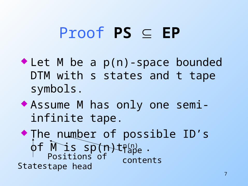
Let M be a p(n)-space bounded DTM with s states and t tape symbols.

Assume M has only one semi-infinite tape.

The number of possible ID’s of M is sp(n)tp(n) .

StatesPositions oftape head

Tapecontents

8

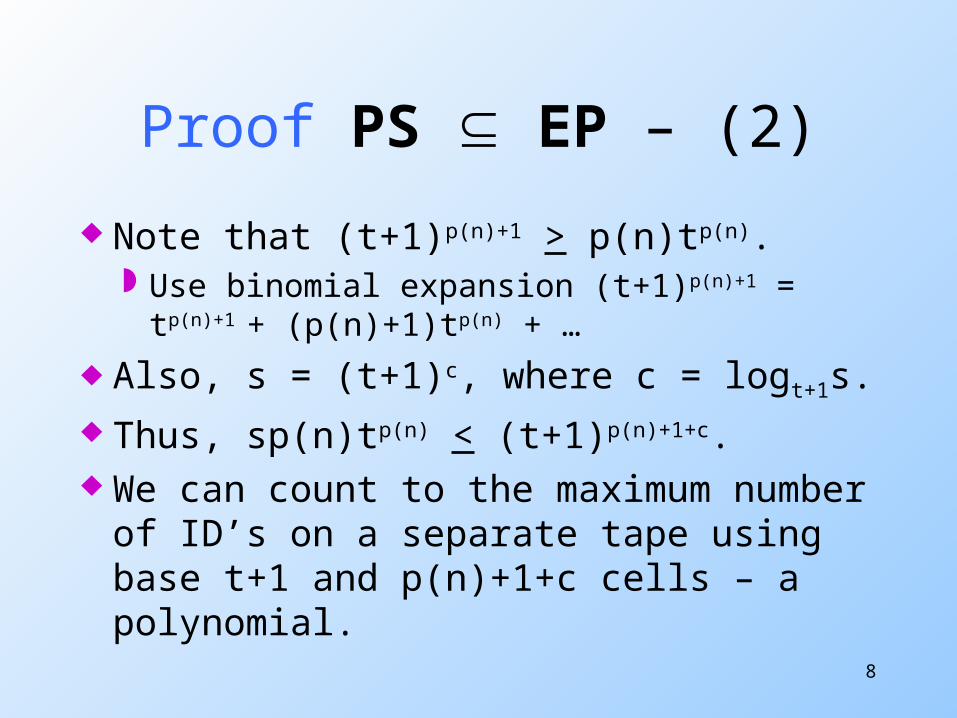
Proof PS EP – (2)

Note that (t+1)p(n)+1 > p(n)tp(n). Use binomial expansion (t+1)p(n)+1 = tp(n)

+1 + (p(n)+1)tp(n) + …

Also, s = (t+1)c, where c = logt+1s. Thus, sp(n)tp(n) < (t+1)p(n)+1+c. We can count to the maximum

number of ID’s on a separate tape using base t+1 and p(n)+1+c cells – a polynomial.

9

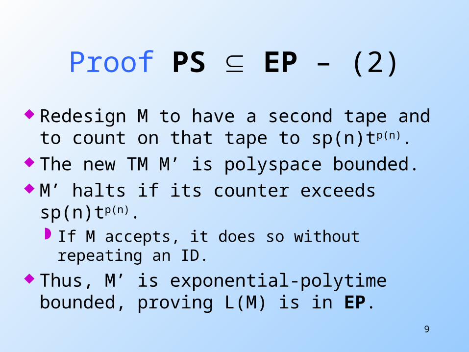
Proof PS EP – (2)

Redesign M to have a second tape and to count on that tape to sp(n)tp(n).

The new TM M’ is polyspace bounded. M’ halts if its counter exceeds

sp(n)tp(n). If M accepts, it does so without repeating

an ID. Thus, M’ is exponential-polytime

bounded, proving L(M) is in EP.

10

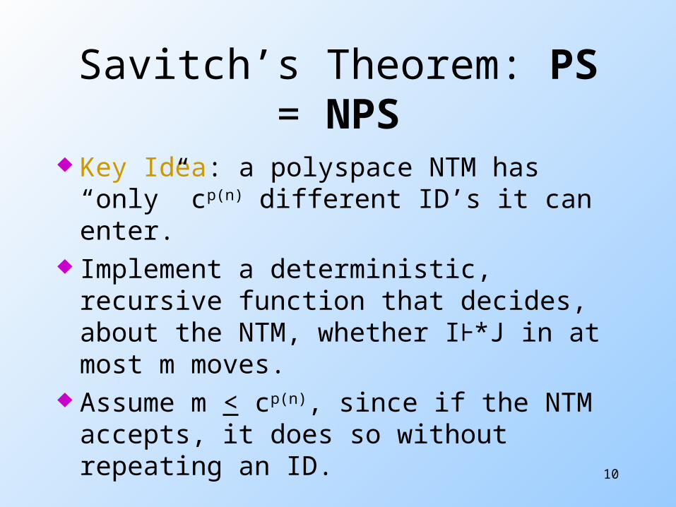
Savitch’s Theorem: PS = NPS

Key Idea: a polyspace NTM has “only” cp(n) different ID’s it can enter.

Implement a deterministic, recursive function that decides, about the NTM, whether I⊦*J in at most m moves.

Assume m < cp(n), since if the NTM accepts, it does so without repeating an ID.

11

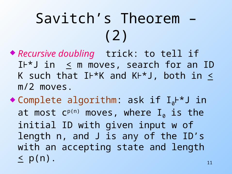
Savitch’s Theorem – (2)

Recursive doubling trick: to tell if I⊦*J in < m moves, search for an ID K such that I⊦*K and K⊦*J, both in < m/2 moves.

Complete algorithm: ask if I0⊦*J in at most cp(n) moves, where I0 is the initial ID with given input w of length n, and J is any of the ID’s with an accepting state and length < p(n).

12

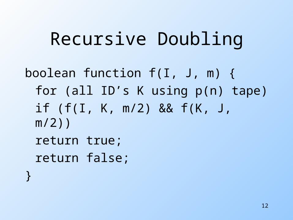
Recursive Doubling

boolean function f(I, J, m) {for (all ID’s K using p(n) tape)

if (f(I, K, m/2) && f(K, J, m/2))return true;

return false;}

13

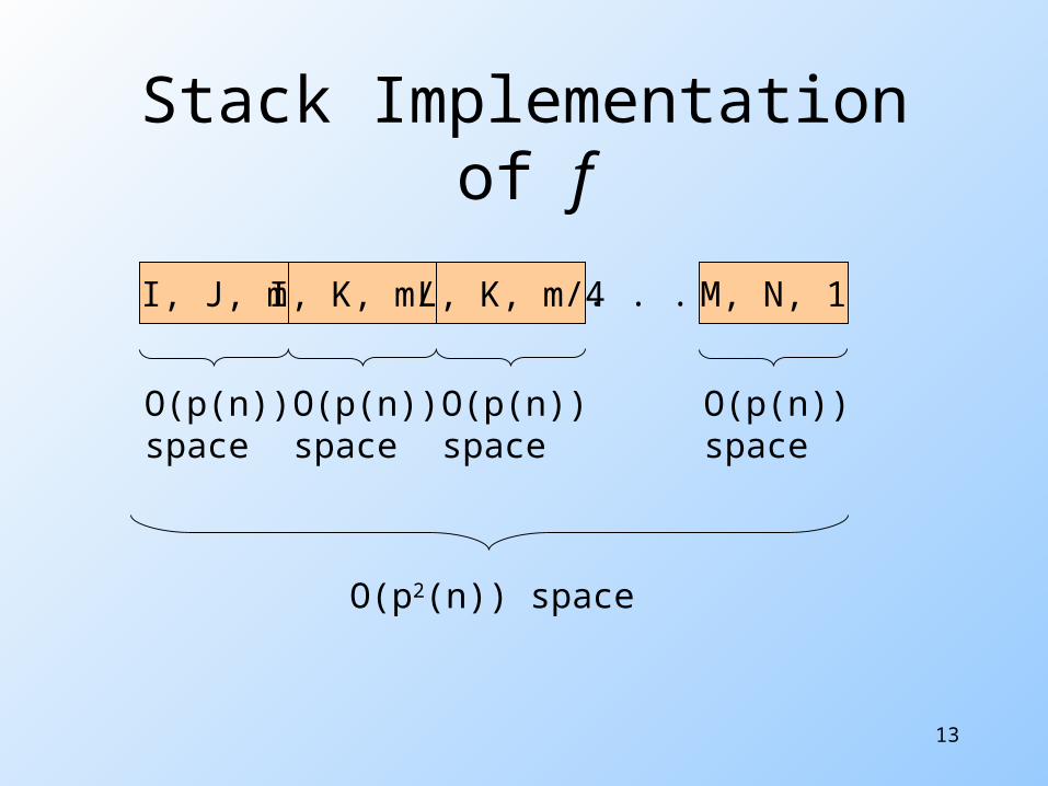
Stack Implementation of f

I, J, m

O(p(n))space

I, K, m/2

O(p(n))space

L, K, m/4

O(p(n))space

M, N, 1

O(p(n))space

. . .

O(p2(n)) space

14

Space for Recursive Doubling

f(I, J, m) requires space O(p(n)) to store I, J, m, and the current K. m need not be more than cp(n), so it

can be stored in O(p(n)) space. How many calls to f can be active

at once? Largest m is cp(n).

15

Space for Recursive Doubling – (2)

Each call with third argument m results in only one call with argument m/2 at any one time.

Thus, at most log2cp(n) = O(p(n)) calls can be active at any one time.

Total space needed by the DTM is therefore O(p2(n)) – a polynomial.

16

PS-Complete Problems

A problem P in PS is said to be PS-complete if there is a polytime reduction from every problem in PS to P.

Note: it has to be polytime, not polyspace, because:1. Polyspace can exponentiate the output size.2. Without polytime, we could not deal with

the question P = PS?

17

What PS-Completeness Buys

If some PS-complete problem is:1. In P, then P = PS.2. In NP, then NP = PS.

18

Quantified Boolean Formulas

We shall meet a PS-complete problem, called QBF : is a given quantified boolean formula true?

But first we meet the QBF’s themselves.

We shall give a recursive (inductive) definition of QBF’s along with the definition of free/bound variable occurrences.

19

QBF’s – (2)

First-order predicate logic, with variables restricted to true/false.

Basis:1. Constants 0 (false) and 1 (true) are

QBF’s.2. A variable is a QBF, and that

variable occurrence is free in this QBF.

20

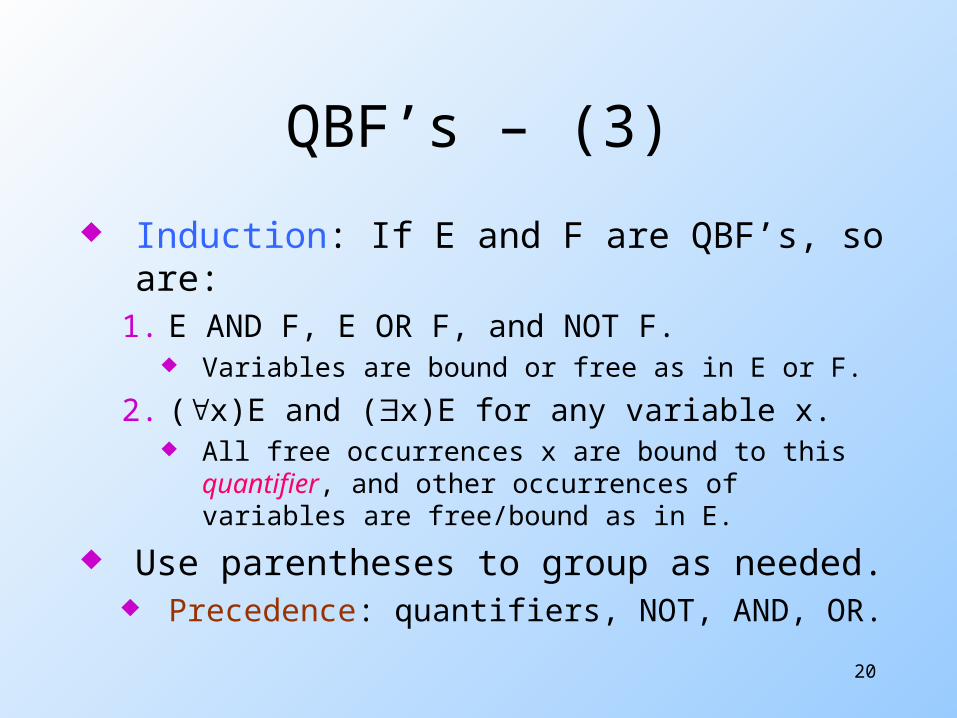
QBF’s – (3)

Induction: If E and F are QBF’s, so are:

1. E AND F, E OR F, and NOT F. Variables are bound or free as in E or F.

2. (x)E and (x)E for any variable x. All free occurrences x are bound to this

quantifier, and other occurrences of variables are free/bound as in E.

Use parentheses to group as needed. Precedence: quantifiers, NOT, AND, OR.

21

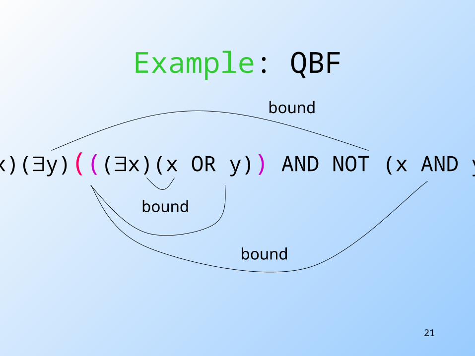
Example: QBF

(x)(y)(((x)(x OR y)) AND NOT (x AND y))

bound

bound

bound

22

Evaluating QBF’s

In general, a QBF is a function from truth assignments for its free variables to {0, 1} (false/true).

Important special case: no free variables; a QBF is either true or false.

We shall give the evaluation only for these formulas.

23

Evaluating QBF’s – (2)

Induction on the number of operators, including quantifiers.

Stage 1: eliminate quantifiers. Stage 2: evaluate variable-free

formulas. Basis: 0 operators.

Expression can only be 0 or 1, because there are no free variables.

Truth value is 0 or 1, respectively.

24

Induction

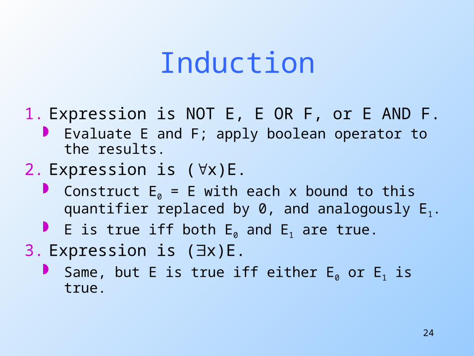
1. Expression is NOT E, E OR F, or E AND F. Evaluate E and F; apply boolean operator to

the results.

2. Expression is (x)E. Construct E0 = E with each x bound to this

quantifier replaced by 0, and analogously E1.

E is true iff both E0 and E1 are true.

3. Expression is (x)E. Same, but E is true iff either E0 or E1 is true.

25

Example: Evaluation

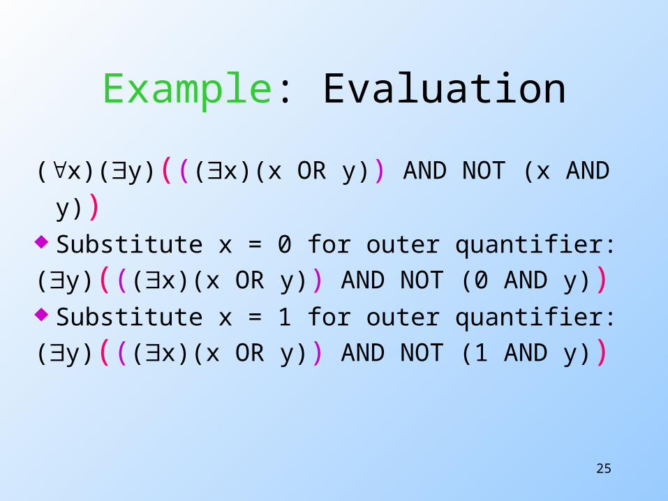
(x)(y)(((x)(x OR y)) AND NOT (x AND

y)) Substitute x = 0 for outer quantifier:(y)(((x)(x OR y)) AND NOT (0 AND y)) Substitute x = 1 for outer quantifier:(y)(((x)(x OR y)) AND NOT (1 AND y))

26

Example: Evaluation – (2)

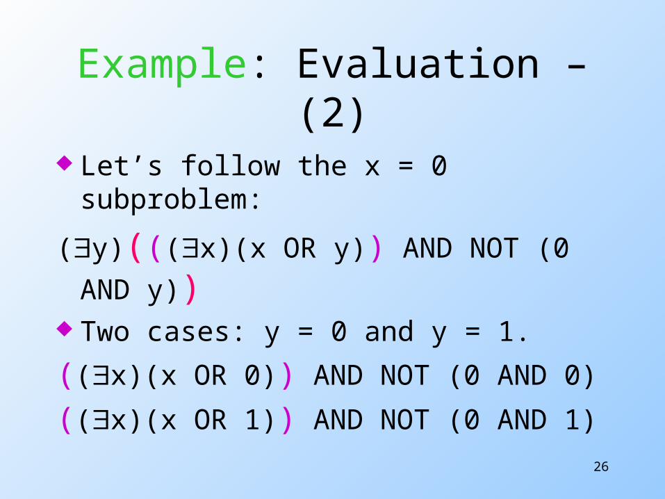
Let’s follow the x = 0 subproblem:

(y)(((x)(x OR y)) AND NOT (0 AND

y)) Two cases: y = 0 and y = 1.

((x)(x OR 0)) AND NOT (0 AND 0)

((x)(x OR 1)) AND NOT (0 AND 1)

27

Example: Evaluation – (3)

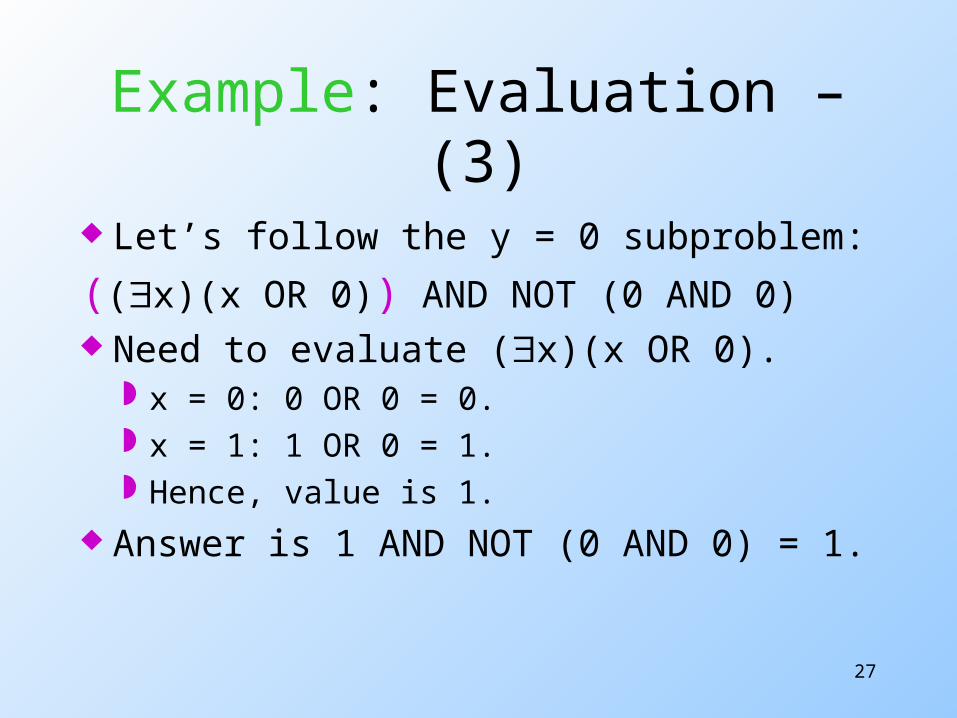
Let’s follow the y = 0 subproblem:

((x)(x OR 0)) AND NOT (0 AND 0) Need to evaluate (x)(x OR 0).

x = 0: 0 OR 0 = 0. x = 1: 1 OR 0 = 1. Hence, value is 1.

Answer is 1 AND NOT (0 AND 0) = 1.

28

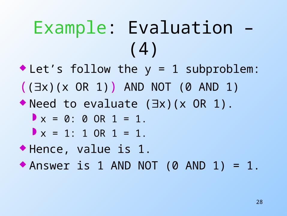
Example: Evaluation – (4)

Let’s follow the y = 1 subproblem:

((x)(x OR 1)) AND NOT (0 AND 1) Need to evaluate (x)(x OR 1).

x = 0: 0 OR 1 = 1. x = 1: 1 OR 1 = 1.

Hence, value is 1. Answer is 1 AND NOT (0 AND 1) =

1.

29

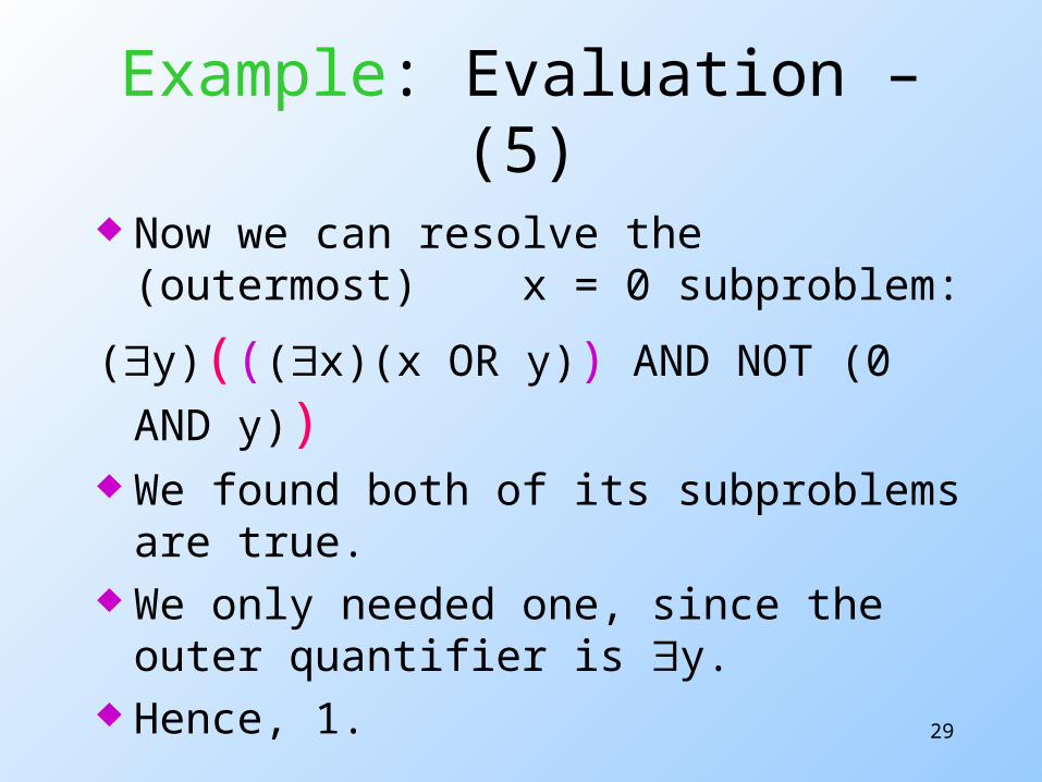
Example: Evaluation – (5)

Now we can resolve the (outermost) x = 0 subproblem:

(y)(((x)(x OR y)) AND NOT (0 AND

y)) We found both of its subproblems

are true. We only needed one, since the

outer quantifier is y. Hence, 1.

30

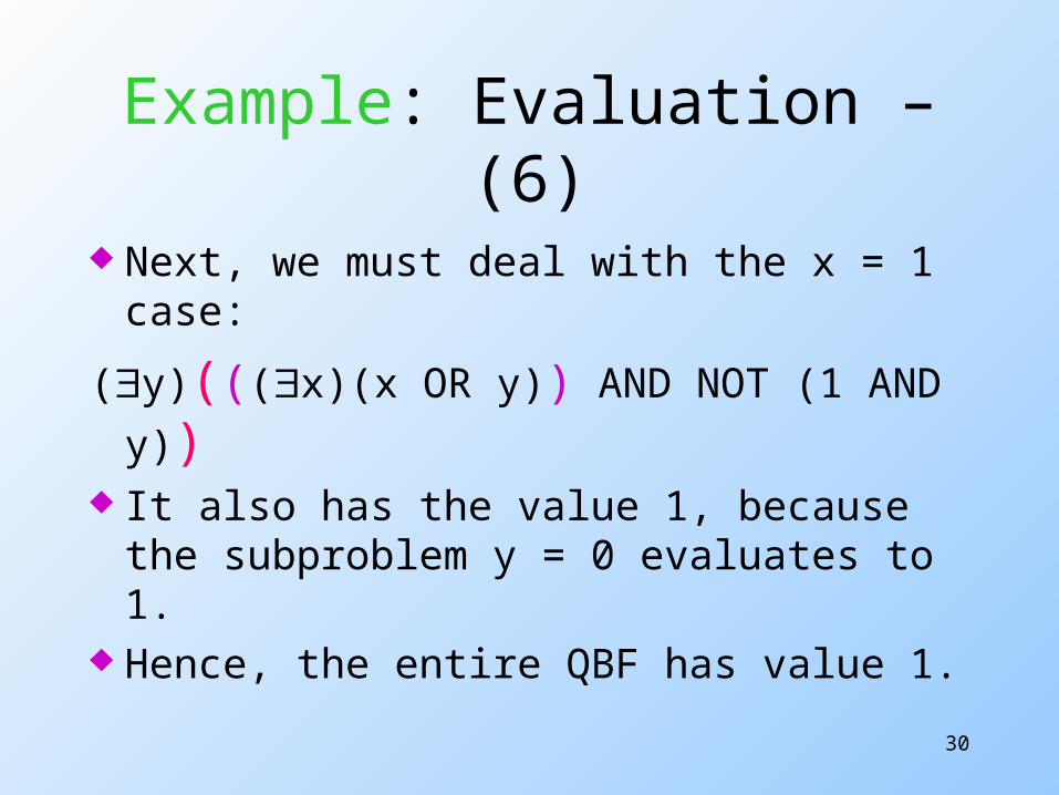
Example: Evaluation – (6)

Next, we must deal with the x = 1 case:

(y)(((x)(x OR y)) AND NOT (1 AND

y)) It also has the value 1, because the

subproblem y = 0 evaluates to 1. Hence, the entire QBF has value 1.

31

The QBF Problem

The problem QBF is: Given a QBF with no free variables, is

its value 1 (true)? Theorem: QBF is PS-complete. Comment: What makes QBF extra

hard? Alternation of quantifiers. Example: if only used, then the

problem is really SAT.

32

Part I: QBF is in PS

Suppose we are given QBF F of length n.

F has at most n operators. We can evaluate F using a stack of

subexpressions that never has more than n subexpressions, each of length < n.

Thus, space used is O(n2).

33

QBF is in PS – (2)

Suppose we have subexpression E on top of the stack, and E = G OR H.

1. Push G onto the stack.2. Evaluate it recursively.3. If true, return true.4. If false, replace G by H, and return

what H returns.

34

QBF is in PS – (3) Cases E = G AND H and E = NOT G

are handled similarly. If E = (x)G, then treat E as if it were

E = E0 OR E1. Observe: difference between and OR

is succinctness; you don’t write both E0 and E1.

• But E0 and E1 must be almost the same.

If E = (x)G, then treat E as if it were E = E0 AND E1.

35

Part II: All of PS Polytime Reduces to QBF

Recall that if a polyspace-bounded TM M accepts its input w of length n, then it does so in cp(n) moves, where c is a constant and p is a polynomial.

Use recursive doubling to construct a QBF saying “there is a sequence of cp(n) moves of M leading to acceptance of w.”

36

Polytime Reduction: The Variables

We need collections of boolean variables that together represent one ID of M.

A variable ID I is a collection of O(p(n)) variables yj,A. True iff the j-th position of the ID I is A

(a state or tape symbol). 0 < j < p(n)+1 = length of an ID.

37

The Variables – (2)

We shall need O(p(n)) variable ID’s. So the total number of boolean

variables is O(p2(n)). Shorthand: (I), where I is a variable

ID, is short for (y1)(y2)(…), where the y’s are the boolean variables belonging to I.

Similarly (I).

38

Structure of the QBF

The QBF is (I0)(If)(S AND N AND F AND U), where:

1. I0 and If are variable ID’s representing the start and accepting ID’s respectively.

2. U = “unique” = one symbol per position.3. S = “starts right”: I0 = q0w.

4. F = “finishes right” = If accepts.

5. N = “moves right.”

39

Structure of U, S, and F

U is as done for Cook’s theorem. S asserts that the first n+1 symbols

of I0 are q0w, and other symbols are blank.

F asserts one of the symbols of If is a final state.

All are easy to write in O(p(n)) time.

40

Structure of QBF N

N(I0,If) needs to say that I0⊦*If by at most cp(n) moves.

We construct subexpressions N0, N1, N2,… where Ni(I,J) says “I⊦*J by at most 2i moves.”

N is Nk, where k = log2cp(n) = O(p(n)). Note: differs from text,

where the subscriptsexponentiate.

41

Constructing the Ni’s

Basis: N0(I, J) says “I=J OR I⊦J.”

If I represents variables yj,A and J represents variables zj,A, we say I=J by the boolean expression for yj,A = zj,A for all j and A. Remember: a=b is

(a AND b) OR (NOT a AND NOT b). I⊦J uses the same idea as for SAT.

42

Induction

Suppose we have constructed Ni and want to construct Ni+1.

Ni+1(I, J) = “there exists K such that Ni(I, K) and Ni(K, J).”

We must be careful: We must write O(p(n)) formulas, each

in polynomial time.

43

Induction – (2)

If each formula used two copies of the previous formula, times and sizes would exponentiate.

Trick: use to make one copy of Ni serve for two.

Ni+1(I, J) = “if (P,Q) = (I,K) or (P,Q) = (K,J), then Ni(P, Q).”

44

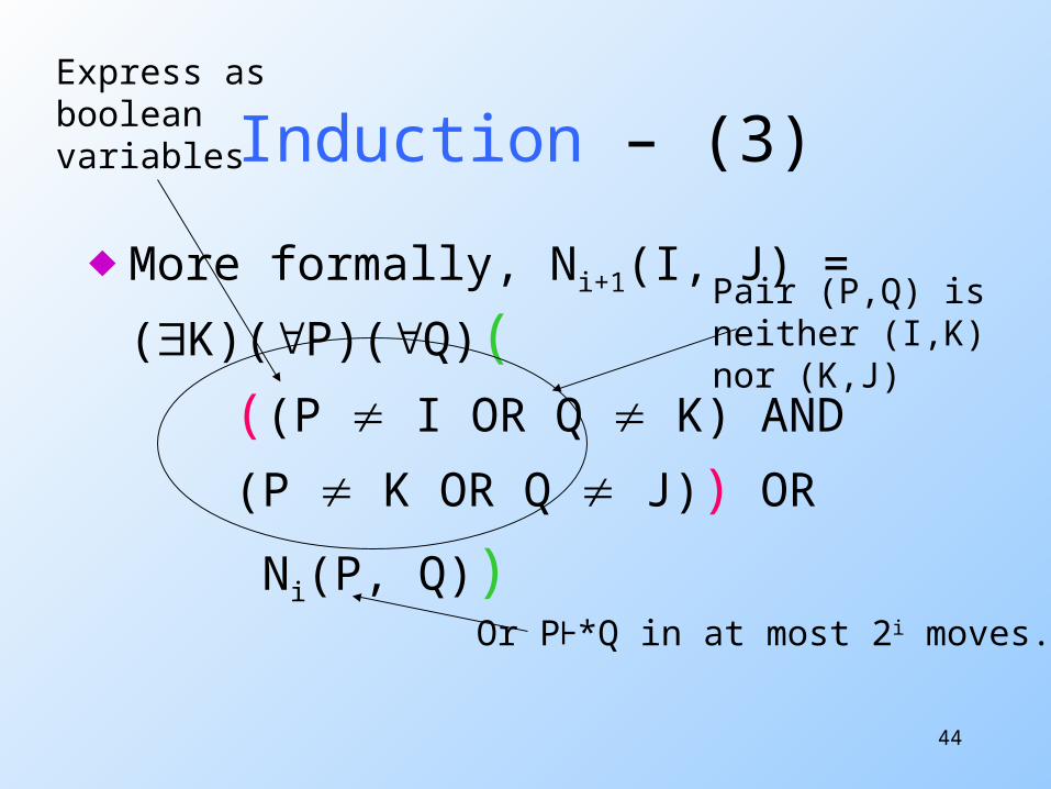
Induction – (3)

More formally, Ni+1(I, J) = (K)(P)

(Q)(((P I OR Q K) AND

(P K OR Q J)) OR

Ni(P, Q))

Express asbooleanvariables

Pair (P,Q) isneither (I,K)nor (K,J)

Or P⊦*Q in at most 2i moves.

45

Induction – (4)

We can thus write Ni+1 in time O(p(n)) plus the time it takes to write Ni.

Remember: N is Nk, where k = log2cp(n) = O(p(n)).

Thus, we can write N in time O(p2(n)). Finished!! The whole QBF for w can be

written in polynomial time.