Embed Size (px)
Citation preview
1
Power System Dynamics as Primal-Dual
Algorithm for Optimal Load ControlChanghong Zhao⇤, Ufuk Topcu†, Na Li‡ and Steven H. Low⇤
⇤Electrical Engineering, California Institute of Technology
{czhao, slow}@caltech.edu† Electrical & Systems Engineering, University of Pennsylvania
[email protected]‡ Control and Dynamical Systems, California Institute of Technology
Abstract
We formulate an optimal load control (OLC) problem in power networks where the objective
is to minimize the aggregate cost of tracking an operating point subject to power balance over the
network. We prove that the swing dynamics and the branch power flows, coupled with frequency-based
load control, serve as a distributed primal-dual algorithm to solve OLC. Even though the system has
multiple equilibrium points, we prove that it nonetheless converges to an optimal point. This result
implies that the local frequency deviations at each bus convey exactly the right information about the
global power imbalance for the loads to make individual decisions that turn out to be globally optimal. It
allows a completely decentralized solution without explicit communication among the buses. Simulations
show that the proposed OLC mechanism can resynchronize bus frequencies with significantly improved
transient performance.
A preliminary version has appeared in the Proceedings of the 3rd IEEE International Conference on Smart Grid Communica-
tions, Tainan City, Taiwan, November 2012.
May 6, 2013 DRAFT
arX
iv:1
305.
0585
v1 [
cs.S
Y]
2 M
ay 2
013
2
I. INTRODUCTION
In power systems, regulation efforts traditionally focus on the generation side. For example,
the automatic generation control adjusts the setpoints of generators based on area frequency
deviations and unscheduled cross-area power flows [1]. To track the given setpoints at a faster
time scale and improve stability, control mechanisms, such as the excitation system, speed
governing system and power system stabilizer, are deployed on the generation side [2][3].
However, relying solely on generation control may not be enough. Due to limited ramping
rate and large inertia, generators are suitable for minute-by-minute power balance, but may
incur expensive wear-and-tear, high emissions, and low thermal efficiency when responding
to regulation signals at intervals of seconds [4][5]. Complementary to generation control, we
consider load control as an additional mechanism that provides fast and inexpensive power system
regulation. Indeed the feasibility and efficiency of load control has already been demonstrated
in several electricity markets. Long Island Power Authority (LIPA) developed LIPAedge, which
provides 24.9 MW of demand reduction and 75 MW of spinning reserve by 23,400 loads [6].
Electric Reliability Council of Texas (ERCOT) has 50% of its 2400 MW reserve provided by
loads. Pennsylvania-New Jersey-Maryland Interconnection (PJM) opens up the regulation market
to participation by loads [4]. While most of the existing programs focus on direct manipulation of
loads in a centralized scheme, the alternative strategy of decentralized load control via frequency
measurement has also been studied in the literatures. Brooks et al. suggests that loads can sense
and respond to frequency and provide regulation within 1 second [5]. Molina-Garcia et al.
studies the aggregate response characteristics when individual loads are turned on/off as the
frequency fluctuates [7]. Donnelly et al. develops proportional control of intelligent loads, and
investigates the effect of distribution systems, the effect of discretized control, and the effect of
time-delay of control actions, through the simulation of a 16-generator transmission network [8].
In our previous papers [9]–[11] we study a decentralized algorithm to minimize the cost of load
control based on local frequency measurement and neighborhood communication. Frequency-
based load control does not require communication to a centralized grid operator, and is thus
suitable for large-scale decentralized deployment.
In this paper we consider a power transmission network where, at steady state, the generator
frequencies at different buses (or in different balancing authorities) are synchronized to the
May 6, 2013 DRAFT
3
same nominal value and the mechanic power is balanced with the electric power at each bus.
Suppose a small change in generation occurs on an arbitrary subset of the buses. How should
the controllable loads in the network be reduced (or increased) in real time in a way that (i)
balances the generation shortfall (or surplus), (ii) resynchronizes the bus frequencies, and (iii)
minimizes a measure of aggregate cost of participation in such a load control? We formalize
this question as an optimal load control (OLC) problem. The basic dynamics at each generation
bus is described by swing equations that relate the imbalance between generation and load to
the rate of frequency change. We assume the change in generation is small and the DC load
flow model is reasonably accurate. We develop a frequency-based load control where loads are
controlled based on locally measured frequency deviations and their individual cost functions.
We prove that this frequency-based load control coupled with the system dynamics serve as
a distributed primal-dual algorithm to solve OLC. Simulation of the IEEE 68-bus test system
shows that the proposed OLC mechanism resynchronize bus frequencies with smaller steady-
state error, smaller overshoot and shorter settling time, compared to the case with only local
generator control mechanisms like power system stabilizers.
The paper is organized as follows. Section II describes a dynamic model of power networks
and formulates OLC. Section III explains how the frequency-based load control and the system
dynamics serve as a distributed primal-dual algorithm to solve OLC and its dual. Section
IV provides the convergence analysis of the primal-dual algorithm. Section V illustrates the
proposed scheme through the simulation of the IEEE 68-bus test system. Section VI concludes
the paper. Section VII provides a detailed justification of our model of the branch power flow,
both analytically and through simulation of the much more detailed dynamic model of power
systems developed in [3][12].
II. PROBLEM FORMULATION
Let R denote the set of real numbers and N denote the set of non-zero natural numbers. For
a set N , let |N | denote its cardinality. A variable without a subscript usually denotes a vector
with appropriate components, e.g., ! = (!
j
, j 2 N ) 2 R|N |. For a, b 2 R, a b, the expression
[·]ba
denotes max {min{·, b}, a}. For a matrix A, let AT denote its transpose. For a signal !(t)
of time, let ! denote its time derivative d!
dt
.
May 6, 2013 DRAFT
4
A. Transmission network model
The power transmission network is described by a graph (N , E) where N = {1, . . . , |N |} is
the set of buses and E ✓ N ⇥N is the set of transmission lines connecting the buses. We make
the following assumptions: 1
• The lines (i, j) 2 E are lossless and characterized by their reactance x
ij
.
• The voltage magnitudes |Vj
| of buses j 2 N are constants.
• Reactive power injections at the buses and reactive power flows on the lines are ignored.
We assume that (N , E) is directed, with an arbitrary orientation, so that if (i, j) 2 E then
(j, i) 62 E . We use (i, j) and i ! j interchangeably to denote a link in E , and use “i : i ! j”
and “k : j ! k” respectively to denote the set of buses i that are predecessors of bus j and
the set of buses k that are successors of bus j. We also assume without loss of generality that
(N , E) is connected.
The network has two types of buses: generator buses and load buses. A generator bus not only
has loads, but also an AC generator that converts mechanic power into electric power through a
rotating prime mover. A load bus has only loads but no generator. We assume that the system is
always under the three-phase balanced condition, and for a bus j 2 N , its phase a voltage at time
t isp2|V
j
| cos(!0t+ ✓
0j
+�✓
j
(t)), where !
0 is the nominal frequency, ✓0j
is the nominal phase
angle, and �✓
j
(t) the time-varying phase angle deviation. The frequency at bus j is defined as
!
j
:= !
0+ �
˙
✓
j
, and we call �!
j
:= �
˙
✓
j
the frequency deviation at bus j. We assume that
the frequency deviations �!
j
are small for all the buses j 2 N and the differences �✓
i
��✓
j
between phase angle deviations are small across all the links (i, j) 2 E . We adopt a standard
dynamic model, e.g., in [2, Section 11.4].
Generator buses. We assume coherency between the internal and terminal (bus) voltage phase
angles of the generator so that these angles always differ by a constant even during the transient,
which is discussed in more detail in Section VII-C. Then the dynamics on a generator bus j is
modeled by the swing equation
M
j
�!
j
+D
0j
�!
j
= P
m
j
0 � P
0loss,j
� P
e
j
,
1These assumptions are similar to the standard DC approximation except that we do not assume the nominal phase angle
difference is small across each link.
May 6, 2013 DRAFT
5
where M
j
> 0 is the inertia constant of the generator. The term D
0j
�!
j
with D
0j
> 0 represents
the deviation in generator power loss due to friction, from its nominal value P
0loss,j
. Here P
m
j
0
is the mechanic power injection to the generator, and P
e
j
is the electric power export of the
generator, which equals the sum of loads on bus j and the net power injection from bus j to
the rest of the network.
In general, load power may depend on both the bus voltage magnitude (which is assumed fixed)
and frequency. We distinguish between two types of loads, frequency-sensitive and frequency-
insensitive. We assume frequency-sensitive (e.g., motor-type) loads increase linearly with fre-
quency deviation and model the aggregate of these loads by ˆ
d
0j
+D
00j
�!
j
with D
00j
> 0, whereˆ
d
0j
is its nominal power. We assume frequency-insensitive loads can be actively controlled and
our goal is to design and analyze these control laws. Let dj
denote the aggregate of frequency-
insensitive loads on bus j. Finally we allow constant power load P
l
j
that is switched on or off.
Then the electric power P e
j
is the sum of frequency-sensitive loads, frequency-insensitive loads,
constant power load, and the net power injection from bus j to other buses:
P
e
j
:=
ˆ
d
0j
+D
00j
�!
j
+ d
j
+ P
l
j
+
X
k:j!k
P
jk
�X
i:i!j
P
ij
where P
jk
is the branch power flow from bus j to bus k.
Hence the dynamics on a generator bus j is
M
j
�!
j
= ��
D
j
�!
j
+ d
j
� P
m
j
+ P
outj
� P
inj
�
where D
j
:= D
0j
+ D
00j
, Pm
j
:= P
m
j
0 � P
0j,loss
� ˆ
d
0j
� P
l
j
, and P
outj
:=
P
k:j!k
P
jk
and P
inj
:=
P
i:i!j
P
ij
are respectively the total branch power flows out and into bus j. Let d
0j
, P
m,0j
, P
0ij
denote the nominal (operating) point at which d
0j
� P
m,0j
+ P
out,0j
��P
in,0j
= 0, and let dj
(t) =
d
0j
+�d
j
(t), P
m
j
(t) = P
m,0j
+�P
m
j
(t), P
ij
(t) = P
0ij
+�P
ij
(t). Then the deviations satisfy
M
j
�!
j
= ��
D
j
�!
j
+�d
j
��P
m
j
+�P
outj
��P
inj
�
. (1)
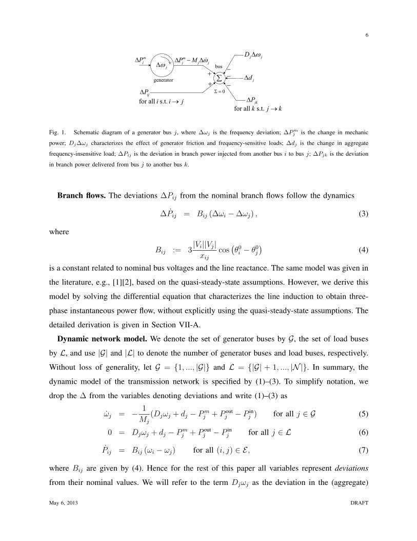
Figure 1 is a schematic diagram of the generator bus model (1).
Load buses. For a load bus that has no generator, there is the following algebraic relation
between the variables introduced above: 2
0 = D
j
�!
j
+�d
j
��P
m
j
+�P
outj
��P
inj
. (2)
2There may be load buses with large inertia that can be modeled by swing dynamics (1) as proposed in [13]. We will treat
them as generator buses mathematically.
May 6, 2013 DRAFT
6
generator
j jD Z'
jd'
jkP'
jZ'
ijP'for all s.t.i i jo
for all s.t.k j ko
bus
¦
06
�� �
��
mj j jP M Z' � ' �m
jP'
Fig. 1. Schematic diagram of a generator bus j, where �!j is the frequency deviation; �Pmj is the change in mechanic
power; Dj�!j characterizes the effect of generator friction and frequency-sensitive loads; �dj is the change in aggregate
frequency-insensitive load; �Pij is the deviation in branch power injected from another bus i to bus j; �Pjk is the deviation
in branch power delivered from bus j to another bus k.
Branch flows. The deviations �P
ij
from the nominal branch flows follow the dynamics
�
˙
P
ij
= B
ij
(�!
i
��!
j
) , (3)
where
B
ij
:= 3
|Vi
||Vj
|x
ij
cos
�
✓
0i
� ✓
0j
�
(4)
is a constant related to nominal bus voltages and the line reactance. The same model was given in
the literature, e.g., [1][2], based on the quasi-steady-state assumptions. However, we derive this
model by solving the differential equation that characterizes the line induction to obtain three-
phase instantaneous power flow, without explicitly using the quasi-steady-state assumptions. The
detailed derivation is given in Section VII-A.
Dynamic network model. We denote the set of generator buses by G, the set of load buses
by L, and use |G| and |L| to denote the number of generator buses and load buses, respectively.
Without loss of generality, let G = {1, ..., |G|} and L = {|G| + 1, ..., |N |}. In summary, the
dynamic model of the transmission network is specified by (1)–(3). To simplify notation, we
drop the � from the variables denoting deviations and write (1)–(3) as
!
j
= � 1
M
j
(D
j
!
j
+ d
j
� P
m
j
+ P
outj
� P
inj
) for all j 2 G (5)
0 = D
j
!
j
+ d
j
� P
m
j
+ P
outj
� P
inj
for all j 2 L (6)
˙
P
ij
= B
ij
(!
i
� !
j
) for all (i, j) 2 E , (7)
where B
ij
are given by (4). Hence for the rest of this paper all variables represent deviations
from their nominal values. We will refer to the term D
j
!
j
as the deviation in the (aggregate)
May 6, 2013 DRAFT
7
frequency-sensitive load even though it also includes the deviation in generator power loss due
to friction. We will refer to the term P
m
j
as the change in generation even though it may also
include changes in constant power loads.
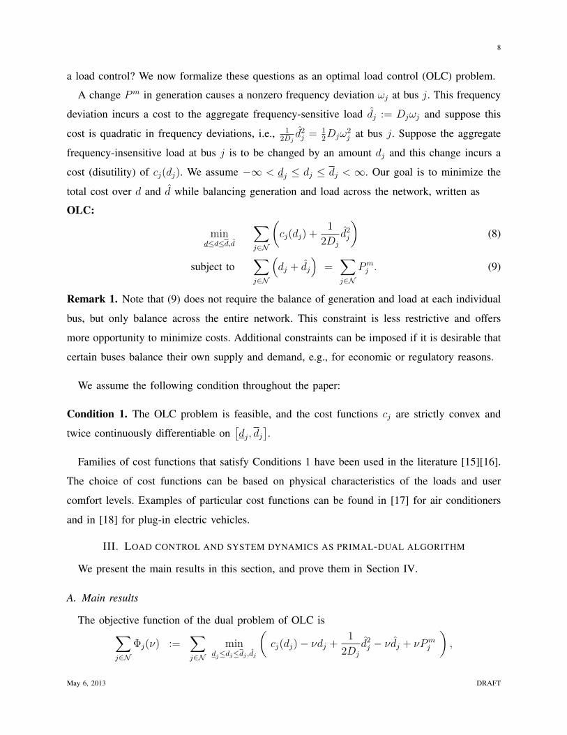
A steady state of the dynamic system described by (5)–(7) is defined as a state in which all
power deviations and frequency deviations are constant over time, !j
= 0 for j 2 G, and ˙
P
ij
= 0
for (i, j) 2 E .
Discussion. The model given by (5)–(7) captures the power system behavior at the timescale
of seconds. In this paper we will only consider a step change in generation (constant deviations
P
m
j
), which implies that the proposed model does not include the action of turbine-governor
(at a similar or slower timescale than the proposed model) that changes the mechanic power
injection in response to frequency deviation to rebalance power. Nor does it include any secondary
frequency control mechanism such as automatic generation control that operates at a much slower
timescale to restore the nominal frequency. This model therefore explores the feasibility of the
active control of frequency-insensitive loads at a fast timescale as a supplement to the turbine-
governor mechanism to resynchronize frequency and rebalance power. Our results in Sections
III and V suggest it is feasible.
The proposed model implicitly assumes that the time for individual frequencies !
j
to resyn-
chronize (converge to a common system frequency, which may be time varying) after a power
imbalance can be similar to the time for them to converge to their equilibrium value (which may
be different from the nominal value). Whether this assumption holds depends on the electrical
distances [14] between different buses. For buses that are close, they resynchronize almost
instantly to a common frequency which then converges more slowly to the equilibrium value. For
buses that are far away, their resynchronization times are similar to convergence times. These
observations are shown by the simulation of a more realistic model; see Figure 9 in Section
VII-C.
B. Optimal load control
Suppose a step change P
m
= (P
m
j
, j 2 N ) in generation is injected to the set N of buses. How
should the frequency-insensitive loads d = (d
j
, j 2 N ) in the network be reduced (or increased)
in real-time in a way that (i) balances the generation shortfall (or surplus), (ii) resynchronizes
the bus frequencies, and (iii) minimizes a measure of aggregate disutility of participation in such
May 6, 2013 DRAFT
8
a load control? We now formalize these questions as an optimal load control (OLC) problem.
A change P
m in generation causes a nonzero frequency deviation !
j
at bus j. This frequency
deviation incurs a cost to the aggregate frequency-sensitive load ˆ
d
j
:= D
j
!
j
and suppose this
cost is quadratic in frequency deviations, i.e., 12Dj
ˆ
d
2j
=
12Dj
!
2j
at bus j. Suppose the aggregate
frequency-insensitive load at bus j is to be changed by an amount dj
and this change incurs a
cost (disutility) of c
j
(d
j
). We assume �1 < d
j
d
j
d
j
< 1. Our goal is to minimize the
total cost over d and ˆ
d while balancing generation and load across the network, written as
OLC:
min
ddd,d
X
j2N
✓
c
j
(d
j
) +
1
2D
j
ˆ
d
2j
◆
(8)
subject toX
j2N
⇣
d
j
+
ˆ
d
j
⌘
=
X
j2N
P
m
j
. (9)
Remark 1. Note that (9) does not require the balance of generation and load at each individual
bus, but only balance across the entire network. This constraint is less restrictive and offers
more opportunity to minimize costs. Additional constraints can be imposed if it is desirable that
certain buses balance their own supply and demand, e.g., for economic or regulatory reasons.
We assume the following condition throughout the paper:
Condition 1. The OLC problem is feasible, and the cost functions c
j
are strictly convex and
twice continuously differentiable on⇥
d
j
, d
j
⇤
.
Families of cost functions that satisfy Conditions 1 have been used in the literature [15][16].
The choice of cost functions can be based on physical characteristics of the loads and user
comfort levels. Examples of particular cost functions can be found in [17] for air conditioners
and in [18] for plug-in electric vehicles.
III. LOAD CONTROL AND SYSTEM DYNAMICS AS PRIMAL-DUAL ALGORITHM
We present the main results in this section, and prove them in Section IV.
A. Main results
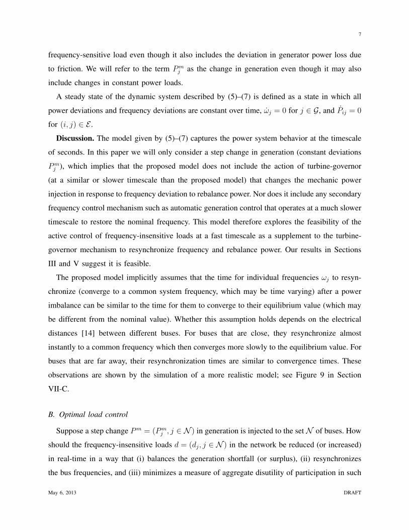
The objective function of the dual problem of OLC isX
j2N
�
j
(⌫) :=
X
j2N
min
djdjdj ,dj
✓
c
j
(d
j
)� ⌫d
j
+
1
2D
j
ˆ
d
2j
� ⌫
ˆ
d
j
+ ⌫P
m
j
◆
,
May 6, 2013 DRAFT
9
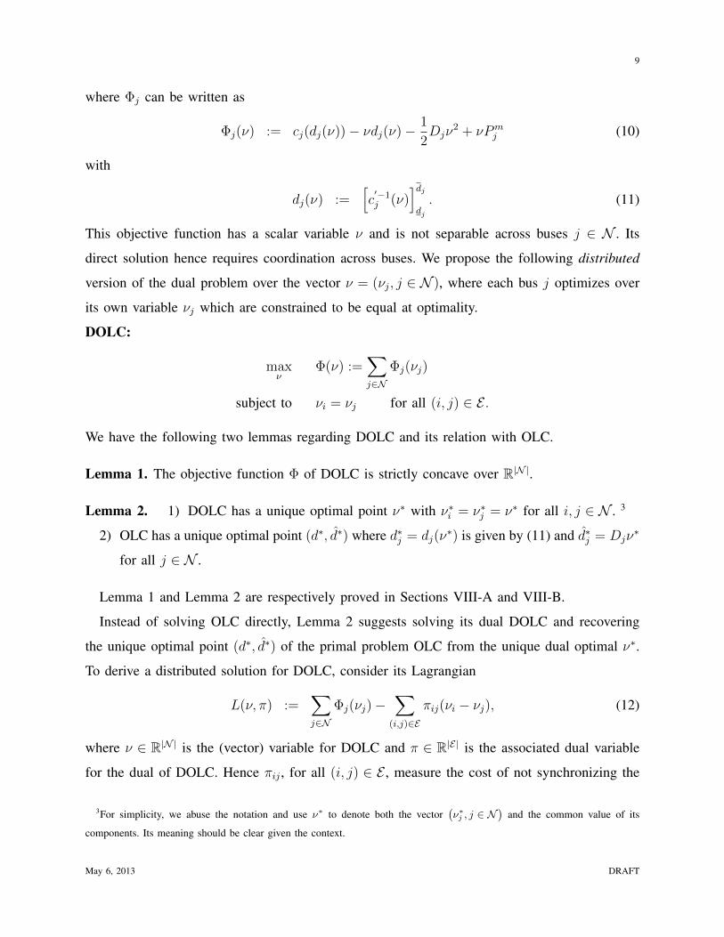
where �
j
can be written as
�
j
(⌫) := c
j
(d
j
(⌫))� ⌫d
j
(⌫)� 1
2
D
j
⌫
2+ ⌫P
m
j
(10)
with
d
j
(⌫) :=
h
c
0�1j
(⌫)
i
dj
dj
. (11)
This objective function has a scalar variable ⌫ and is not separable across buses j 2 N . Its
direct solution hence requires coordination across buses. We propose the following distributed
version of the dual problem over the vector ⌫ = (⌫
j
, j 2 N ), where each bus j optimizes over
its own variable ⌫
j
which are constrained to be equal at optimality.
DOLC:
max
⌫
�(⌫) :=
X
j2N
�
j
(⌫
j
)
subject to ⌫
i
= ⌫
j
for all (i, j) 2 E .
We have the following two lemmas regarding DOLC and its relation with OLC.
Lemma 1. The objective function � of DOLC is strictly concave over R|N |.
Lemma 2. 1) DOLC has a unique optimal point ⌫⇤ with ⌫
⇤i
= ⌫
⇤j
= ⌫
⇤ for all i, j 2 N . 3
2) OLC has a unique optimal point (d⇤, ˆd⇤) where d
⇤j
= d
j
(⌫
⇤) is given by (11) and ˆ
d
⇤j
= D
j
⌫
⇤
for all j 2 N .
Lemma 1 and Lemma 2 are respectively proved in Sections VIII-A and VIII-B.
Instead of solving OLC directly, Lemma 2 suggests solving its dual DOLC and recovering
the unique optimal point (d⇤, ˆd⇤) of the primal problem OLC from the unique dual optimal ⌫⇤.
To derive a distributed solution for DOLC, consider its Lagrangian
L(⌫, ⇡) :=
X
j2N
�
j
(⌫
j
)�X
(i,j)2E
⇡
ij
(⌫
i
� ⌫
j
), (12)
where ⌫ 2 R|N | is the (vector) variable for DOLC and ⇡ 2 R|E| is the associated dual variable
for the dual of DOLC. Hence ⇡
ij
, for all (i, j) 2 E , measure the cost of not synchronizing the
3For simplicity, we abuse the notation and use ⌫⇤ to denote both the vector�⌫⇤j , j 2 N
�and the common value of its
components. Its meaning should be clear given the context.
May 6, 2013 DRAFT
10
variables ⌫
i
and ⌫
j
across buses i and j. Using (10)–(12), a partial primal-dual algorithm for
DOLC takes the form
⌫
j
= �
j
@L
@⌫
j
(⌫, ⇡) = ��
j
�
d
j
(⌫
j
) +D
j
⌫
j
� P
m
j
+ ⇡
outj
� ⇡
inj
�
for j 2 G (13)
0 =
@L
@⌫
j
(⌫, ⇡) = ��
d
j
(⌫
j
) +D
j
⌫
j
� P
m
j
+ ⇡
outj
� ⇡
inj
�
for j 2 L (14)
⇡
ij
= �⇠
ij
@L
@⇡
ij
(⌫, ⇡) = ⇠
ij
(⌫
i
� ⌫
j
) for (i, j) 2 E , (15)
where �
j
> 0, ⇠ij
> 0 are stepsizes and ⇡
outj
:=
P
k:j!k
⇡
jk
, ⇡inj
:=
P
i:i!j
⇡
ij
. We interpret
(13)–(15) as an algorithm iterating on the primal variables ⌫ and dual variables ⇡ over time
t � 0 as follows. For a generator bus j, given the current iterate (⌫(t), ⇡(t)), one can use
�
j
@L (⌫(t), ⇡(t)) /@⌫
j
as the rate of change in ⌫
j
. For a load bus j, the current iterate ⌫
j
(t) is
obtained as the solution of
@L
@⌫
j
(⌫
j
, ⌫�j
(t), ⇡(t)) = 0
given ⇡(t) and ⌫�j
(t) := (⌫
i
(t), i 6= j). For a link (i, j) 2 E , given the current iterate (⌫(t), ⇡(t)),
one can use �⇠
ij
@L (⌫(t), ⇡(t)) /@⇡
ij
as the rate of change in ⇡
ij
.
In (13)–(15), the stepsizes �
i
and ⇠
ij
can take any positive values, and the initial values
(⌫(0), ⇡(0)) can also be taken arbitrarily. In particular, let
�
j
= M
�1j
, ⇠
ij
= B
ij
,
and
⌫(0) = !(0), ⇡(0) = P (0),
where !(0) and P (0) are the frequency deviations and branch flow deviations at t = 0, the
instant right after a step change P
m in generation has occurred. We use continuous time t as
the iterating time in the primal-dual algorithm (13)–(15), and get a trajectory (⌫(t), ⇡(t)) for
t � 0. We compare it with (!(t), P (t)), the trajectory of frequency deviations and branch flow
deviations, and find that the the two trajectories take the same value for all t. Mathematically,
(13)–(15) is identical to (5)–(7), if we identify ⌫ with ! and ⇡ with P , and take d
j
= d
j
(!
j
) in
(5)–(6).
May 6, 2013 DRAFT
11
For convenience, we collect here the system dynamics and load control:
!
j
= � 1
M
j
⇣
d
j
+
ˆ
d
j
� P
m
j
+ P
outj
� P
inj
⌘
for j 2 G (16)
0 = d
j
+
ˆ
d
j
� P
m
j
+ P
outj
� P
inj
for j 2 L (17)
˙
P
ij
= B
ij
(!
i
� !
j
) for (i, j) 2 E (18)
ˆ
d
j
= D
j
!
j
for j 2 N (19)
d
j
=
h
c
0�1j
(!
j
)
i
dj
dj
for j 2 N . (20)
The dynamics (16)–(19) are automatically carried out by the power system while the active con-
trol (20) needs to be implemented at each frequency-insensitive load. Let (d(t), ˆd(t),!(t), P (t))
denote a trajectory of frequency-insensitive loads, frequency-sensitive loads, frequency deviations
and branch flow deviations, generated by the dynamics (16)–(20) of the load-controlled system.
Theorem 1. Every trajectory (d(t),
ˆ
d(t),!(t), P (t)) generated by (16)–(20) converges to a limit
(d
⇤,
ˆ
d
⇤,!
⇤, P
⇤) as t ! 1 such that
1) (d
⇤,
ˆ
d
⇤) is the unique vector of optimal load control for OLC;
2) !
⇤ is the unique vector of optimal frequency deviations for DOLC;
3) P
⇤ is a vector of optimal branch flows for the dual of DOLC.
We will prove Theorem 1 and other results in Section IV below.
B. Implications
Our main results have several important implications:
1) Frequency-based load control: The frequency-insensitive loads can be controlled using
their individual marginal cost functions according to (20), based only on frequency devi-
ations !
j
(t) (from their nominal values) that are measured at their local buses. Note that
both the load control here and the generator droop control [1] respond to the difference
between the nominal frequency and the actual frequency, but they are complementary. Load
control is activated immediately after a sudden generation-load imbalance because many
loads can respond quickly. Droop control is slower than load control due to larger time
constants associated with valves and prime movers, but it compensates for a large amount
of generation-load imbalance to prevent the frequency from wandering outside the desired
May 6, 2013 DRAFT

12
limit. Optimal load control explicitly uses cost functions of individual loads to share the
required load reduction/increase optimally among all loads in the network, whereas in
droop control generator outputs are adjusted proportionally to frequency deviations so that
the sum of implicit cost functions which are quadratic in the changes of generator outputs
is minimized.
2) Complete decentralization. The common operating frequency is a global signal that mea-
sures the power imbalance across the entire network. Our result implies that the local
frequency deviation !
j
(t) at each bus turns out to convey exactly the right information
about the global power imbalance for the loads themselves to make optimal decisions
based on their own marginal cost functions. That is, with the right information, their local
decisions turn out to be globally optimal. This result allows a completely decentralized
solution without explicit communication among the buses.
3) Reverse engineering of swing dynamics. The frequency-based load control (20) coupled
with the dynamics (16)–(19) of swing equations and branch power flows serve as a
distributed primal-dual algorithm to solve OLC and its dual DOLC.
4) Frequency and branch flows. In the context of optimal load control, the frequency devi-
ations !
j
(t) emerge as the Lagrange multipliers of OLC that measure the cost of power
imbalance, whereas the branch flow deviations P
ij
(t) emerge as the Lagrange multipliers
of DOLC that measure the cost of frequency asynchronism.
5) Uniqueness of solution. Lemma 2 implies that the optimal frequency !
⇤ is unique and
hence the optimal load control (d⇤, ˆd⇤) is unique. As we show below, the optimal branch
flows P
⇤ are unique if and only if the network is a tree. Theorem 1 says nonetheless,
that, even for mesh networks, any trajectory generated by the load control and system
dynamics indeed converges to an optimal point, with the optimal value of P
⇤ dependent
on the initial condition right after a change in generation.
6) Optimal frequency. The structure of DOLC indicates that the frequencies at all the buses are
synchronized at optimality even though they can be different during transient. However, the
common frequency deviation !
⇤ at optimality is in general nonzero. This implies that while
frequency-based load control and the swing dynamics can resynchronize bus frequencies to
a unique common value after a change in generation, the new frequency may be different
from the common operating frequency before the change. To respect the tight frequency
May 6, 2013 DRAFT
13
regulation limits in power systems, the new steady-state frequency deviation should be
made small. Simulations in Section V show that the new steady-state frequency deviations
are reasonably small with OLC. Other mechanisms, such as isochronous generators [1] or
automatic generation control [2], will be needed to drive the new operating frequency to
its nominal value, through, e.g., integral control of the frequency deviation.
Of course, many of these insights are well known; our results merely provide a fresh and unified
interpretation within an optimization framework for frequency-based load control.
IV. CONVERGENCE ANALYSIS
This section is devoted to the proof of Theorem 1 and other properties as given by Theorems
2 – 3 below. Before going into the details, we first sketch out the key steps in establishing
Theorem 1, the convergence of the trajectories generated by (16)–(20).
1) Theorem 2: The set of optimal points (!
⇤, P
⇤) of DOLC and its dual and the set of
equilibrium points of (16)–(20) are nonempty and the same. Denote both of them by Z
⇤.
2) Theorem 3: If (N , E) is a tree network, Z⇤ is a singleton with a unique equilibrium point
(!
⇤, P
⇤), otherwise (if (N , E) is a mesh network), Z⇤ has an uncountably infinite number
(a subspace) of equilibria with the same !
⇤ but different P ⇤.
3) Theorem 1: We use a Lyapunov-type technique to prove that every trajectory (!(t), P (t))
generated by (16)–(20) approaches a nonempty, compact subset Z
+ of Z
⇤ as t ! 1.
Hence, if (N , E) is a tree network, it is straightforward from Theorem 3 that any trajectory
(!(t), P (t)) converges to the unique optimal point (!⇤, P
⇤). If (N , E) is a mesh network,
we show with a more careful argument that (!(t), P (t)) still converges to a point in Z
+,
as opposed to wandering around Z
+. Theorem 1 then follows from Lemma 2.
We now elaborate on these ideas.
Given !, the optimal loads (d, ˆd) are uniquely determined by (19)–(20), hence we focus on the
variables (!, P ). Let C be the |N |⇥|E| incidence matrix with C
je
= 1 if e = (j, k) 2 E for some
bus k 2 N , Cje
= �1 if e = (i, j) 2 E for some bus i 2 N , and C
je
= 0 otherwise. Recall that
we assumed that the first |G| buses {1, . . . , |G|} are generator buses and the remaining |L| buses
{|G|+ 1, . . . , |N |} are load buses. Decompose C into an |G|⇥ |E| submatrix CG corresponding
to generator buses and an |L|⇥ |E| submatrix CL corresponding to load buses, i.e., C =
⇥
CGCL
⇤
.
May 6, 2013 DRAFT
14
Similarly, let !G and !L respectively denote the vector of frequency deviations at generator buses
and load buses, so !
T
=
⇥
!
T
G !
T
L⇤
. Let
�G(!G) :=
X
j2G
�
j
(!
j
) and LG(!G, P ) := �G(!G)� !
T
GCGP,
�L(!L) :=
X
j2L
�
j
(!
j
) and LL(!L, P ) := �L(!L)� !
T
LCLP.
Identifying ⌫ with ! and ⇡ with P , we can rewrite the Lagrangian for DOLC defined in (12),
in terms of !G and !L, as
L(!, P ) = �(!)� !
T
CP = LG(!G, P ) + LL(!L, P ). (21)
Then (16)–(20) (equivalently, (13)–(15)) can be rewritten in the vector form as
!G = �G
@LG
@!G(!G, P )
�
T
= �G
@�G
@!G(!G)
�
T
� CGP
!
(22)
0 =
@LL
@!L(!L, P ) =
@�L
@!L(!L)
�
T
� CLP (23)
˙
P = �⌅
@L
@P
(!, P )
�
T
= ⌅C
T
! (24)
where �G := diag(�j
, j 2 G) and ⌅ := diag(⇠ij
, (i, j) 2 E). The differential algebraic equations
(22)–(24) describe the dynamics of the power network when active load control is performed.
A pair (!⇤, P
⇤) is called a saddle point of L if
L(!, P
⇤) L(!
⇤, P
⇤) L(!
⇤, P ) for all (!, P ). (25)
By [19, Section 5.4.2], (!⇤, P
⇤) is primal-dual optimal for DOLC and its dual if and only if
it is a saddle point of L(!, P ). The following theorem establishes the equivalence between the
primal-dual optimal points and the equilibrium points of (22)–(24).
Theorem 2. A point (!⇤, P
⇤) is primal-dual optimal for DOLC and its dual if and only if it
is an equilibrium point of (22)–(24). Moreover, at least one primal-dual optimal point (!⇤, P
⇤)
exists and !
⇤ is unique among all possible points (!
⇤, P
⇤) that are primal-dual optimal.
Proof: Recall that we identified ⌫ with ! and ⇡ with P . In DOLC, the objective function �
is (strictly) concave over R|N | (by Lemma 1), its constraints are linear, and a finite optimal !⇤
is attained (by Lemma 2). These facts imply that there is no duality gap between DOLC and its
May 6, 2013 DRAFT
15
dual, and there exists a dual optimal point P ⇤ [19, Section 5.2.3]. Moreover, (!⇤, P
⇤) is optimal
for DOLC and its dual if and only if the following Karush-Kuhn-Tucker (KKT) conditions [19,
Section 5.5.3] are satisfied:
Stationarity:@�
@!
(!
⇤) = (CP
⇤)
T (26)
Primal feasibility: !
⇤i
= !
⇤j
for all (i, j) 2 E . (27)
On the other hand, (!⇤, P
⇤) = (!
⇤G,!
⇤L, P
⇤) is an equilibrium point of (22)–(24) if and only if
@�G
@!G(!
⇤T )
�
T
= CGP⇤
@�L
@!L(!
⇤L)
�
T
= CLP⇤
⌅C
T
!
⇤= 0,
which are identical to (26)–(27). Hence, (!⇤, P
⇤) is primal-dual optimal if and only if it is an
equilibrium point of (22)–(24). The uniqueness of !⇤ is given by Lemma 2.
From Lemma 2, we denote the unique optimal point of DOLC by !
⇤1N =
⇥
!
⇤1G!
⇤1L
⇤
, where
1N 2 R|N | , 1G 2 R|G| and 1L 2 R|L| have all their elements equal to 1. From (26)–(27), define
the nonempty set of equilibrium points of (22)–(24) (equivalently, primal-dual optimal points of
DOLC and its dual) as
Z
⇤:=
(
(!, P ) | ! = !
⇤1N , CP =
@�
@!
(!
⇤1N )
�
T
)
. (28)
Let (!⇤1N , P
⇤) = (!
⇤1G,!
⇤1L, P
⇤) 2 Z
⇤ be any equilibrium point of (22)–(24). We consider a
candidate Lyapunov function
U(!, P ) =
1
2
(!G � !
⇤1G)
T
�
�1G (!G � !
⇤1G) +
1
2
(P � P
⇤)
T
⌅
�1(P � P
⇤) . (29)
Obviously U(!, P ) � 0 for all (!, P ) with equality if and only if !G = !
⇤1G and P = P
⇤. We
will show below that ˙
U(!, P ) 0 for all (!, P ), where ˙
U denotes the derivative of U along
the trajectory (!(t), P (t)).
Even though U depends explicitly only on !G and P , ˙
U depends on !L as well through (24).
However, it will prove convenient to express ˙
U as a function of only !G and P . To this end, write
(23) as F (!L, P ) = 0. Then @F
@!L(!L, P ) =
@
2�L@!
2L(!L) is nonsingular for all (!L, P ) from the
May 6, 2013 DRAFT
16
proof of Lemma 1 in Section VIII-A. By the inverse function theorem [20], !L can be written
as a continuously differentiable function of P , denoted by !L(P ), with
@!L
@P
(P ) =
✓
@
2�L
@!
2L
(!L(P ))
◆�1
CL. (30)
Then we can rewrite the Lagrangian L(!, P ) as a function of only (!G, P ) as
L(!, P ) = LG(!G, P ) + LL (!L(P ), P ) =
˜
L (!G, P ) . (31)
We have the following lemma, proved in VIII-C, regarding the properties of ˜
L.
Lemma 3. ˜
L is strictly concave in !G and convex in P .
Rewrite (22)–(24) as
!G = �G
"
@
˜
L
@!G(!G, P )
#
T
(32)
˙
P = �⌅
"
@
˜
L
@P
(!G, P )
#
T
. (33)
Then the derivative of U along any trajectory (!(t), P (t)) generated by (22)–(24) is
˙
U(!, P ) = (!G � !
⇤1G)
T
�
�1G !G + (P � P
⇤)
T
⌅
�1˙
P
=
@
˜
L
@!G(!G, P ) (!G � !
⇤1G)�
@
˜
L
@P
(!G, P ) (P � P
⇤) (34)
˜
L (!G, P )� ˜
L (!
⇤1G, P ) +
˜
L(!G, P⇤)� ˜
L (!G, P ) (35)
= L (!G,!⇤1L, P
⇤)� ˜
L (!
⇤1G, P ) (36)
L (!
⇤1N , P )� ˜
L (!
⇤1G, P ) (37)
= LG (!⇤1G, P ) + LL (!
⇤1L, P )� [LG (!
⇤1G, P ) + LL (!L(P ), P )]
0. (38)
Here (34) follows from (32)–(33). The inequality in (35) results from Lemma 3. The equality
in (36) holds since !L(P⇤) = !
⇤1L by (26). The inequality in (37) is due to L (!G,!
⇤1L, P
⇤)
L (!
⇤1N , P
⇤) L (!
⇤1N , P ) by the saddle point condition (25). The inequality in (38) follows
since !L(P ) is the maximizer of LL (·, P ) given P , by the concavity of LL in !L and the
definition of !L(P ).
May 6, 2013 DRAFT
17
The next lemma, proved in Section VIII-D, characterizes the set in which the value of U does
not change over time.
Lemma 4. ˙
U(!, P ) = 0 if and only if either of the following two conditions holds.
1)
!G = !
⇤1G and CLP =
@�L
@!L(!
⇤1L)
�
T
. (39)
2)
!G = !
⇤1G and !L(P ) = !
⇤1L. (40)
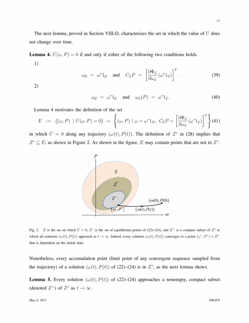
Lemma 4 motivates the definition of the set
E := {(!, P ) | ˙
U(!, P ) = 0} =
(
(!, P ) | ! = !
⇤1N , CLP =
@�L
@!L(!
⇤1L)
�
T
)
(41)
in which ˙
U = 0 along any trajectory (!(t), P (t)). The definition of Z
⇤ in (28) implies that
Z
⇤ ✓ E, as shown in Figure 2. As shown in the figure, E may contain points that are not in Z
⇤.
P
E
Z *Z
Z �
� �(0), (0)PZ
� �* *PZ
� �(0), (0)PZ
� �( ) ( )t P tZZ
� �,PZ � �( ), ( )t P tZ
Fig. 2. E is the set on which U = 0, Z⇤ is the set of equilibrium points of (22)–(24), and Z+ is a compact subset of Z⇤ to
which all solutions (!(t), P (t)) approach as t ! 1. Indeed, every solution (!(t), P (t)) converges to a point (!⇤, P ⇤) 2 Z+
that is dependent on the initial state.
Nonetheless, every accumulation point (limit point of any convergent sequence sampled from
the trajectory) of a solution (!(t), P (t)) of (22)–(24) is in Z
⇤, as the next lemma shows.
Lemma 5. Every solution (!(t), P (t)) of (22)–(24) approaches a nonempty, compact subset
(denoted Z
+) of Z⇤ as t ! 1.
May 6, 2013 DRAFT
18
The proof of Lemma 5 is given in Section VIII-E. The sets Z
+ ✓ Z
⇤ ✓ E are illustrated in
Figure 2. Lemma 5 only guarantees that (!(t), P (t)) approaches Z
+ as t ! 1, but does not
guarantee that it converges to any point in Z
⇤. We now show that (!(t), P (t)) indeed converges
to an equilibrium point in Z
+. Indeed, the convergence is immediate in the special simple case
when Z
⇤ is a singleton, but needs a more careful argument when Z
⇤ has multiple points. The
next theorem reveals the relation between the number of points in Z
⇤ and the network topology.
Theorem 3. 1) Suppose (N , E) is a tree, then Z
⇤ is a singleton.
2) Suppose (N , E) is a mesh (i.e., contains a cycle if regarded as an undirected graph), then
Z
⇤ has an uncountably infinite number of points with the same !
⇤ but different P ⇤.
Proof: Recall that any point (!⇤, P
⇤) 2 Z
⇤ is a solution of (26)–(27). Let h⇤:= CP
⇤=
⇥
@�@!
(!
⇤)
⇤
T . Let ˜
C be the (|N |�1)⇥ |E| reduced incidence matrix obtained from C by removing
any one of its rows. Then ˜
C has a full row rank of |N | � 1 [21]. Consider the corresponding
equation
˜
CP
⇤=
˜
h
⇤ (42)
where ˜
h
⇤ is obtained from h
⇤ by removing the corresponding row. Since !
⇤ is unique, so is ˜
h
⇤.
If (N , E) is a tree, then |E| = |N | � 1. Hence ˜
C is square and invertible, so P
⇤ is unique. If
(N , E) is a (connected) mesh, then |E| > |N | � 1, so ˜
C has a nontrivial null space and there
are uncountably many P
⇤ that solves (42).
With all the results above, we can now finish the proof of Theorem 1.
Proof of Theorem 1: For the case in which (N , E) is a tree, Lemma 5 and Theorem 3(1)
guarantees that every trajectory(!(t), P (t)) converges to the unique primal-dual optimal point
(!
⇤, P
⇤) of DOLC and its dual, which, by Lemma 2, immediately implies Theorem 1.
For the case in which (N , E) is a mesh, since ˙
U(!, P ) 0 for all (!, P ), any solution
(!(t), P (t)) for t � 0 stays in the compact set {(!, P )|U(!, P ) U(!(0), P (0))}. Hence there
exists a convergent subsequence {(!(tk
), P (t
k
)), k 2 N}, where 0 t1 < t2 < ... and t
k
! 1
as k ! 1, such that limk!1 !(t
k
) = !
1 and lim
k!1 P (t
k
) = P
1 for some (!
1, P
1). Lemma
5 implies that (!1, P
1) 2 Z
+ ✓ Z
⇤, and hence !
1= !
⇤1N by (28). Recall that the Lyapunov
function U in (29) can be defined in terms of any equilibrium point (!⇤, P
⇤) 2 Z
⇤. In particular,
May 6, 2013 DRAFT
19
select (!⇤, P
⇤) = (!
1, P
1), i.e.,
U(!, P ) :=
1
2
(!G � !
⇤1G)
T
�
�1G (!G � !
⇤1G) +
1
2
(P � P
1)
T
⌅
�1(P � P
1) .
Since U � 0 and ˙
U 0 along all trajectories (!(t), P (t)), U (!(t), P (t)) must converge as
t ! 1. Moreover it converges to 0 due to the continuity of U in both ! and P :
lim
t!1U (!(t), P (t)) = lim
k!1U (!(t
k
), P (t
k
)) = U (!
1, P
1) = 0.
The equation above implies that the trajectory (!(t), P (t)) converges to (!
1, P
1) 2 Z
+ ✓ Z
⇤,
a primal-dual optimal point for DOLC and its dual. Theorem 1 then follows from Lemma 2.
Remark 2. The standard technique of using a Lyapunov function that is quadratic in primal-dual
variables was first proposed by Arrow et al. [22], and has been revisited many times, e.g., in
[23] [24]. We apply a variation of this general technique to our particular problem and extend
the results in the literature. First, with the algebraic equation (23) in the system, we take a
Lyapunov function candidate that is quadratic in part of the primal variables !G and the dual
variables P , and show that it is indeed a Lyapunov function. Second, in the case when there are
a subspace of equilibrium points due to the non-tree topology of the network, we show that the
system trajectory converges to one of the equilibrium points instead of oscillating around the
equilibrium set, without any modifications to the primal-dual algorithm like those in [24].
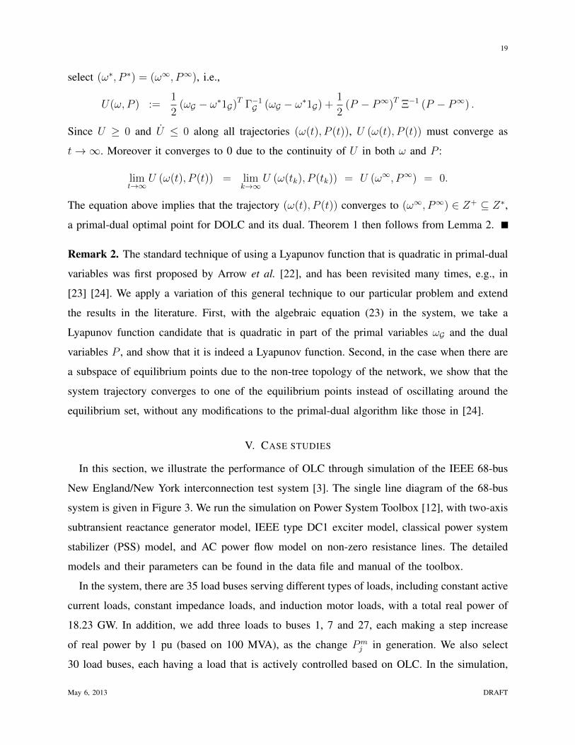
V. CASE STUDIES
In this section, we illustrate the performance of OLC through simulation of the IEEE 68-bus
New England/New York interconnection test system [3]. The single line diagram of the 68-bus
system is given in Figure 3. We run the simulation on Power System Toolbox [12], with two-axis
subtransient reactance generator model, IEEE type DC1 exciter model, classical power system
stabilizer (PSS) model, and AC power flow model on non-zero resistance lines. The detailed
models and their parameters can be found in the data file and manual of the toolbox.
In the system, there are 35 load buses serving different types of loads, including constant active
current loads, constant impedance loads, and induction motor loads, with a total real power of
18.23 GW. In addition, we add three loads to buses 1, 7 and 27, each making a step increase
of real power by 1 pu (based on 100 MVA), as the change P
m
j
in generation. We also select
30 load buses, each having a load that is actively controlled based on OLC. In the simulation,
May 6, 2013 DRAFT
20
Fig. 3. Single line diagram of the 68-bus New England/New York test system.
we take the same bounds⇥
d, d
⇤
with d = �d for each of the 30 controllable loads, and call
the value of 30 ⇥ d the total size of controllable loads. We will show simulation results with
different sizes of controllable loads below. In the simulation, the cost function of a controllable
load d
j
is defined as c
j
(d
j
) = d
2j
/(2↵), with the same ↵ over all the loads. As an example,
we select ↵ = 100 pu. To incorporate some practical consideration, the loads are not controlled
continuously over time. Instead, they measure local frequencies and control their power every
250 ms, which takes a relatively conservative estimate for the rate of load control [25].
Since we have theoretically proved that OLC drives the system to a steady state where the cost
of load control is minimized and total generation and total load are balanced, in the simulation we
mainly focus on the transient performance, specifically, how the frequency and voltage change
after a change in generation. We also look at how effective OLC is as a complement to the
existing control mechanisms, such as the power system stabilizer (PSS), by enabling/disabling
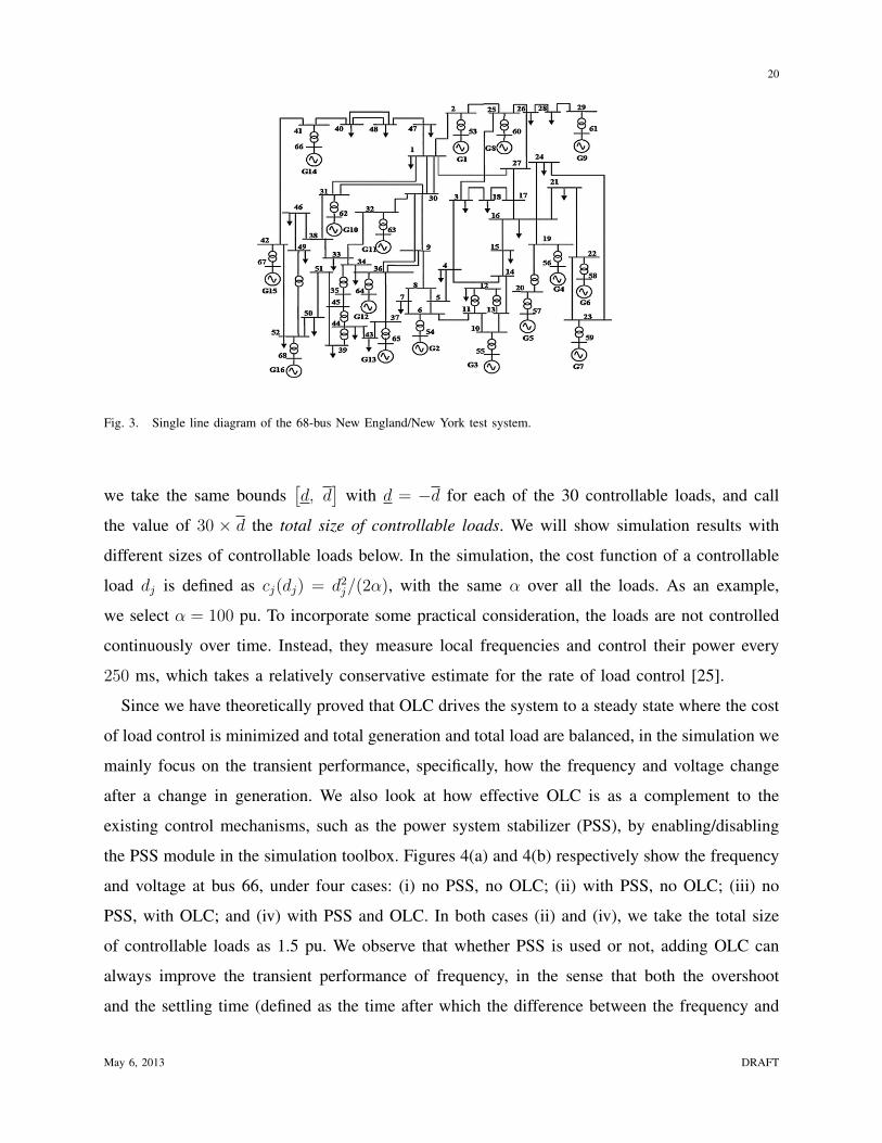
the PSS module in the simulation toolbox. Figures 4(a) and 4(b) respectively show the frequency
and voltage at bus 66, under four cases: (i) no PSS, no OLC; (ii) with PSS, no OLC; (iii) no
PSS, with OLC; and (iv) with PSS and OLC. In both cases (ii) and (iv), we take the total size
of controllable loads as 1.5 pu. We observe that whether PSS is used or not, adding OLC can
always improve the transient performance of frequency, in the sense that both the overshoot
and the settling time (defined as the time after which the difference between the frequency and
May 6, 2013 DRAFT
21
0 5 10 15 20 25 30 3559.94
59.95
59.96
59.97
59.98
59.99
60
60.01Frequency at bus 66
Time (s)
Freq
uenc
y (H
z)
no PSS, no OLCPSS, no OLCno PSS, OLCPSS, OLC
OLC
no OLC
(a)
0 5 10 15 20 25 30 350.992
0.993
0.994
0.995
0.996
0.997
0.998
0.999
1
1.001Voltage at bus 66
Time (s)
Volta
ge (p
u)
no PSS, no OLCPSS, no OLCno PSS, OLCPSS, OLC
OLC
no OLC
(b)
Fig. 4. The (a) frequency and (b) voltage at bus 66, under four cases: (i) no PSS, no OLC; (ii) with PSS, no OLC; (iii) no
PSS, with OLC; (iv) with PSS and OLC.
its new steady-state value never goes beyond 5% of the difference between its old and new
steady-state values) are decreased. Using OLC also leads to a smaller steady-state frequency
error. Comparison between cases (ii) and (iii) also suggests that using OLC solely without
PSS produces a much better performance than using PSS solely without OLC. However the
improvement of the transient performance of voltage is not as significant as frequency, which
may be due to the fact that voltage depends more on reactive power injections while here OLC
does not control the reactive power of loads. The effect of reactive load control to support voltage
will be investigated in future work.
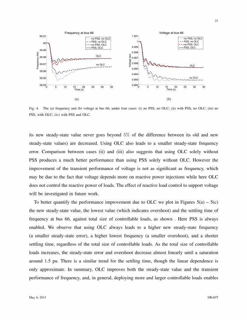
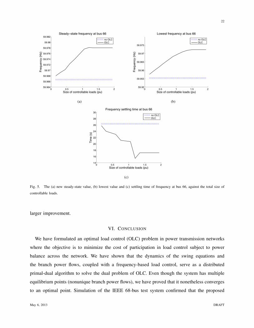
To better quantify the performance improvement due to OLC we plot in Figures 5(a) – 5(c)
the new steady-state value, the lowest value (which indicates overshoot) and the settling time of
frequency at bus 66, against total size of controllable loads, as shown . Here PSS is always
enabled. We observe that using OLC always leads to a higher new steady-state frequency
(a smaller steady-state error), a higher lowest frequency (a smaller overshoot), and a shorter
settling time, regardless of the total size of controllable loads. As the total size of controllable
loads increases, the steady-state error and overshoot decrease almost linearly until a saturation
around 1.5 pu. There is a similar trend for the settling time, though the linear dependence is
only approximate. In summary, OLC improves both the steady-state value and the transient
performance of frequency, and, in general, deploying more and larger controllable loads enables
May 6, 2013 DRAFT
22
0 0.5 1 1.5 259.964
59.966
59.968
59.97
59.972
59.974
59.976
59.978
59.98
59.982Steady−state frequency at bus 66
Size of controllable loads (pu)
Freq
uenc
y (H
z)
no OLCOLC
(a)
0 0.5 1 1.5 259.95
59.955
59.96
59.965
59.97
59.975
Lowest frequency at bus 66
Size of controllable loads (pu)
Freq
uenc
y (H
z)
no OLCOLC
(b)
0 0.5 1 1.5 214
16
18
20
22
24
26
28
30Frequency settling time at bus 66
Size of controllable loads (pu)
Tim
e (s
)
no OLCOLC
(c)
Fig. 5. The (a) new steady-state value, (b) lowest value and (c) settling time of frequency at bus 66, against the total size of
controllable loads.
larger improvement.
VI. CONCLUSION
We have formulated an optimal load control (OLC) problem in power transmission networks
where the objective is to minimize the cost of participation in load control subject to power
balance across the network. We have shown that the dynamics of the swing equations and
the branch power flows, coupled with a frequency-based load control, serve as a distributed
primal-dual algorithm to solve the dual problem of OLC. Even though the system has multiple
equilibrium points (nonunique branch power flows), we have proved that it nonetheless converges
to an optimal point. Simulation of the IEEE 68-bus test system confirmed that the proposed
May 6, 2013 DRAFT
23
mechanism can resynchronize bus frequencies with significantly improved transient performance
compared to using only local generator control mechanisms.
ACKNOWLEDGMENT
We thank Ross Baldick, Janusz Bialek, Jeremy Lin, Lang Tong, and Felix Wu for very helpful
discussions on our dynamic network model. We also thank Lijun Chen for discussions on our
approach and Alec Brooks of AeroVironment for suggestions on practical issues. This work is
supported by NSF NetSE grant CNS 0911041, ARPA-E grant de-ar0000226, Southern California
Edison, National Science Council of Taiwan R.O.C. grant NSC 101-3113-P-008-001, NSF CNS
Award 1312390, the Caltech Resnick Institute, and the Okawa Foundation.
VII. APPENDIX: MODELING DETAILS
In this section, we first derive the branch flow dynamic model given by (3)–(4). Then, to show
the accuracy of the model introduced in Section II-A (referred to as “the analytic model”), we
use a more realistic simulation model developed in [3][12] (the same one we used in Section
V) as a benchmark and demonstrate that the analytic model is a reasonable approximation of
the simulation model. The key conclusions from simulations are summarized as follows:
1) The internal and terminal voltage phase angles of the generator swing coherently, i.e., the
rotating speed of a generator is always the same as the frequency at the generator bus.
2) Different buses may have their own frequencies and buses that are far apart in electrical
distance resynchronize at a similar timescale as the convergence time.
3) The simulation model and the analytic model exhibit similar transient behaviors and steady
state values of bus frequencies and branch power flows.
A. Derivation of the branch flow model
We assume that the system is always under the three-phase balanced condition, the frequency
deviations �!
j
are small, and the differences �✓
i
� �✓
j
between phase angle deviations are
small across all the links (i, j) 2 E . Specifically, �!
j
is negligible compared to !
0, and an
approximation of a quantity to the first order of �✓
i
��✓
j
is reasonable. Now we show that the
deviations �P
ij
in three-phase instantaneous power flows from their nominal values follow the
dynamics in (3)–(4), by solving the differential equation that characterizes the line induction.
May 6, 2013 DRAFT
24
Without loss of generality suppose that buses i and j are wye-connected [2] and each of the
three lines has the same inductance L and zero resistance. Let the phase a voltages at buses i and
j at time t be v
a
i
(t) =
p2|V
i
| cos(!0t+ ✓
0i
+�✓
i
(t)) and v
a
j
(t) =
p2|V
j
| cos(!0t+ ✓
0j
+�✓
j
(t))
respectively, and assume the voltage magnitudes are fixed. Denote the phase a current from i to
j at time t by i
a
ij
(t).
For t 0, suppose �✓
j
(t) = 0 for all the buses j. Hence the system is at a steady state with
i
a
ij
(t) =
p2|I0| cos(!0
t+ ✓
0c
). From phasor calculations we have
|I0| =|V0|x
ij
✓
0c
= tan
�1
|Vj
| cos ✓0j
� |Vi
| cos ✓0i
|Vi
| sin ✓0i
� |Vj
| sin ✓0j
�
where x
ij
:= !
0L, and |V0| :=
q
|Vi
|2 + |Vj
|2 � 2|Vi
||Vj
| cos(✓0i
� ✓
0j
). Then, we have
i
a
ij
(0) =
p2|I0| cos ✓0
c
=
p2
�
|Vi
| sin ✓0i
� |Vj
| sin ✓0j
�
x
ij
. (43)
For t � 0, we have
L
di
a
ij
dt
= v
a
i
� v
a
j
,
whose solution is
i
a
ij
(t) =i
a
ij
(0) +
1
L
Z
t
0
�
v
a
i
(⌧)� v
a
j
(⌧)
�
d⌧
⇡i
a
ij
(0) +
p2
!
0L
⇥
|Vi
| sin�
!
0t+ ✓
0i
+�✓
i
(t)
�
� |Vi
| sin ✓0i
⇤
�p2
!
0L
⇥
|Vj
| sin�
!
0t+ ✓
0j
+�✓
j
(t)
�
� |Vj
| sin ✓0j
⇤
=
p2
x
ij
⇥
|Vi
| sin�
!
0t+ ✓
0i
+�✓
i
(t)
�
� |Vj
| sin�
!
0t+ ✓
0j
+�✓
j
(t)
�⇤
,
(44)
where the approximate equality is due to the assumption that � ˙
✓
j
= �!
j
are negligible compared
to !
0, and the last equality is due to (43).
May 6, 2013 DRAFT
25
From (44) the instantaneous real power injection from i to j at phase a is
p
a
ij
=v
a
i
i
a
ij
=2
|Vi
|2
x
ij
sin
�
!
0t+ ✓
0i
+�✓
i
�
cos
�
!
0t+ ✓
0i
+�✓
i
�
� 2
|Vi
||Vj
|x
ij
sin
�
!
0t+ ✓
0j
+�✓
j
�
cos
�
!
0t+ ✓
0i
+�✓
i
�
=
|Vi
|2
x
ij
sin
�
2!
0t+ 2✓
0i
+ 2�✓
i
�
+
|Vi
||Vj
|x
ij
sin
�
✓
0i
� ✓
0j
+�✓
i
��✓
j
�
� |Vi
||Vj
|x
ij
sin
�
2!
0t+ ✓
0i
+ ✓
0j
+�✓
i
+�✓
j
�
.
(45)
Since we assumed the system is under the three-phase balanced condition, replacing ✓
0i
and ✓
0j
in (45) with ✓
0i
� 23⇡ and ✓
0j
� 23⇡, we get pb
ij
; replacing ✓
0i
and ✓
0j
in (45) with ✓
0i
+
23⇡ and
✓
0j
+
23⇡, we get pc
ij
. Hence the three-phase instantaneous real power flow is (to the first order
of �✓
i
��✓
j
)
P
ij
= p
a
ij
+ p
b
ij
+ p
c
ij
= 3
|Vi
||Vj
|x
ij
sin
�
✓
0i
� ✓
0j
+�✓
i
��✓
j
�
⇡ P
0ij
+�P
ij
(46)
where
P
0ij
= 3
|Vi
||Vj
|x
ij
sin(✓
0i
� ✓
0j
)
is the nominal branch power flow, and
�P
ij
= 3
|Vi
||Vj
|x
ij
cos(✓
0i
� ✓
0j
)(�✓
i
��✓
j
)
is the deviation in branch power flow. By �!
i
= �
˙
✓
i
,�!
j
= �
˙
✓
j
, we get the branch flow
dynamics in (3)–(4).
B. Power flow behavior
In Sections VII-B, VII-C, and VII-D, we first simulate the IEEE 68-bus test system to a steady
state (called “pre-change steady state”) and then introduce the same step change in generation
as in Section V. Then we compare the post-change behavior of the simulation with prediction
of the analytic model introduced in Section II-A.
May 6, 2013 DRAFT
26
We first check the branch flow dynamic model (3)–(4), which was derived above. Repeat it
here as
�
˙
P
ij
= B
ij
(�!
i
��!
j
) for (i, j) 2 E (47)
where B
ij
= 3|Vi
||Vj
| cos�
✓
0i
� ✓
0j
�
/x
ij
is a constant under the assumption of constant voltage
magnitudes and zero line resistances. We use the pre-change steady-state voltage magnitudes
|Vi
|, |Vj
| and angles ✓
0i
, ✓0j
from the simulation to determine B
ij
. Post change, we substitute
the frequency deviations �!
i
(t) from the simulation into (47) to compute the trajectory P
ij
(t)
that would result if �
˙
P
ij
is indeed proportional to the frequency difference, and compare it
with the P
ij
(t) trajectory from the simulation. Since the simulation model is more detailed than
the analytic model (1)–(2) for generator and load buses, using �!
i
(t) from the simulation to
calculate P
ij
(t) isolates the behavior of branch flow modeled by (47).
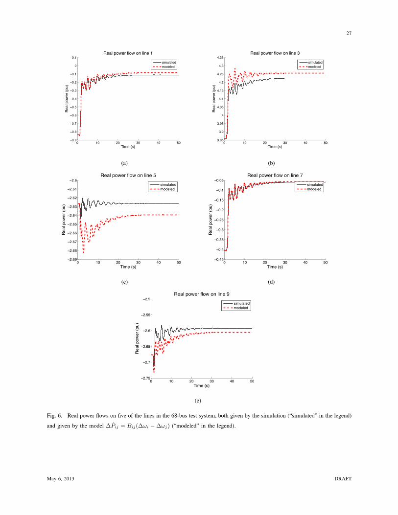
The results are shown in Figures 6(a)–6(e) on five lines. The simulation model and the model
given by (47) exhibit similar transient behaviors and steady state values, suggesting that (47) is
a reasonable approximation of the simulation model.
Specifically, to quantitative the accuracy of steady state, define the steady-state error as
steady-state error :=|fmodeled � fsimulated|
|fsimulated|⇥ 100%,
where “steady-state” refers to the post-change steady state, fmodeled refers to the steady-state
frequency predicted by (47), and fsimulated refers to the steady-state frequency given by the
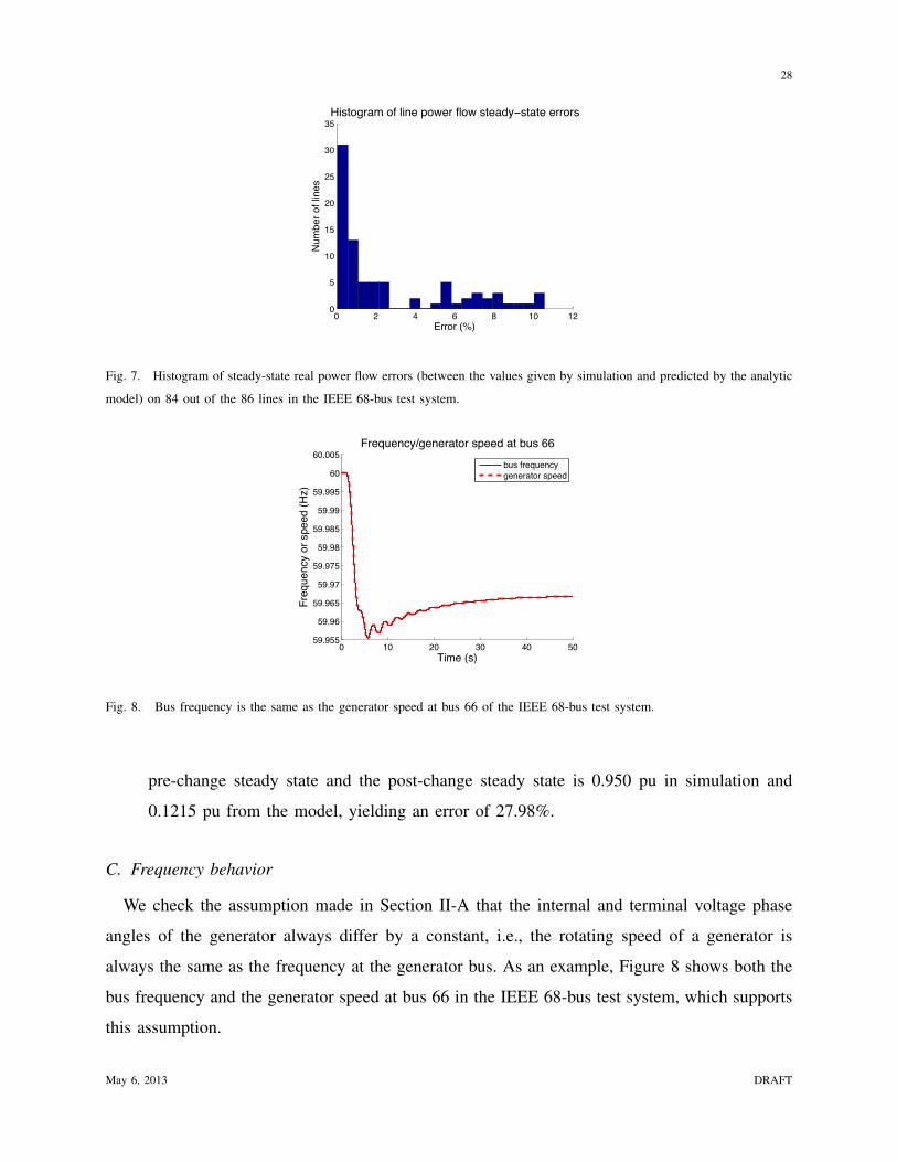
simulation. Figure 7 shows the errors on 84 of the 86 lines in the test system. Of these 84
lines, all errors are within 11% and most within 2%.
The two lines whose errors are not included in Figure 7 are the following:
1) Line from buses 1 to 2: simulated power flow is -0.1105 pu; modeled power flow is -0.0836
pu; steady-state error is 24.35%. However the effect of the change in generation at steady
state is similar between the simulation and the model prediction: the difference between
pre-change steady state and the post-change steady state is 0.7258 pu in simulation and
0.7527 pu from the model, yielding an error of 3.71%.
2) Line from buses 52 to 42: simulated power flow is -0.0068 pu; modeled power flow is
0.0198 pu; steady-state error is 393%. Note that the steady-state values themselves are
much smaller than the average value (about 5pu). Moreover the difference between the
May 6, 2013 DRAFT
27
0 10 20 30 40 50−0.9
−0.8
−0.7
−0.6
−0.5
−0.4
−0.3
−0.2
−0.1
0
0.1Real power flow on line 1
Time (s)
Rea
l pow
er (p
u)
simulatedmodeled
(a)
0 10 20 30 40 503.85
3.9
3.95
4
4.05
4.1
4.15
4.2
4.25
4.3
4.35Real power flow on line 3
Time (s)
Rea
l pow
er (p
u)
simulatedmodeled
(b)
0 10 20 30 40 50−2.69
−2.68
−2.67
−2.66
−2.65
−2.64
−2.63
−2.62
−2.61
−2.6Real power flow on line 5
Time (s)
Rea
l pow
er (p
u)
simulatedmodeled
(c)
0 10 20 30 40 50−0.45
−0.4
−0.35
−0.3
−0.25
−0.2
−0.15
−0.1
−0.05Real power flow on line 7
Time (s)
Rea
l pow
er (p
u)
simulatedmodeled
(d)
0 10 20 30 40 50−2.75
−2.7
−2.65
−2.6
−2.55
−2.5Real power flow on line 9
Time (s)
Rea
l pow
er (p
u)
simulatedmodeled
(e)
Fig. 6. Real power flows on five of the lines in the 68-bus test system, both given by the simulation (“simulated” in the legend)
and given by the model �Pij = Bij(�!i ��!j) (“modeled” in the legend).
May 6, 2013 DRAFT
28
0 2 4 6 8 10 120
5
10
15
20
25
30
35Histogram of line power flow steady−state errors
Error (%)N
umbe
r of l
ines
Fig. 7. Histogram of steady-state real power flow errors (between the values given by simulation and predicted by the analytic
model) on 84 out of the 86 lines in the IEEE 68-bus test system.
0 10 20 30 40 5059.955
59.96
59.965
59.97
59.975
59.98
59.985
59.99
59.995
60
60.005Frequency/generator speed at bus 66
Time (s)
Freq
uenc
y or
spe
ed (H
z)
bus frequencygenerator speed
Fig. 8. Bus frequency is the same as the generator speed at bus 66 of the IEEE 68-bus test system.
pre-change steady state and the post-change steady state is 0.950 pu in simulation and
0.1215 pu from the model, yielding an error of 27.98%.
C. Frequency behavior
We check the assumption made in Section II-A that the internal and terminal voltage phase
angles of the generator always differ by a constant, i.e., the rotating speed of a generator is
always the same as the frequency at the generator bus. As an example, Figure 8 shows both the
bus frequency and the generator speed at bus 66 in the IEEE 68-bus test system, which supports
this assumption.
May 6, 2013 DRAFT
29
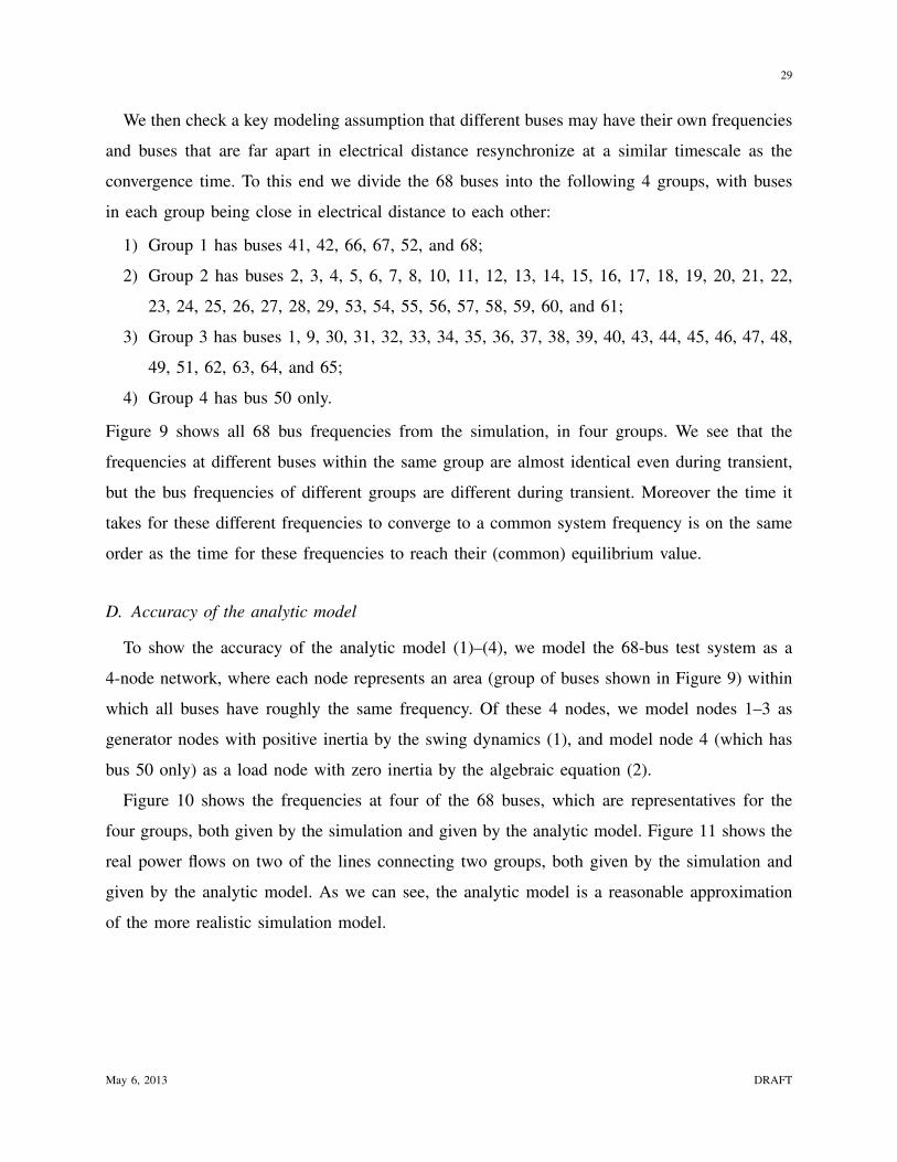
We then check a key modeling assumption that different buses may have their own frequencies
and buses that are far apart in electrical distance resynchronize at a similar timescale as the
convergence time. To this end we divide the 68 buses into the following 4 groups, with buses
in each group being close in electrical distance to each other:
1) Group 1 has buses 41, 42, 66, 67, 52, and 68;
2) Group 2 has buses 2, 3, 4, 5, 6, 7, 8, 10, 11, 12, 13, 14, 15, 16, 17, 18, 19, 20, 21, 22,
23, 24, 25, 26, 27, 28, 29, 53, 54, 55, 56, 57, 58, 59, 60, and 61;
3) Group 3 has buses 1, 9, 30, 31, 32, 33, 34, 35, 36, 37, 38, 39, 40, 43, 44, 45, 46, 47, 48,
49, 51, 62, 63, 64, and 65;
4) Group 4 has bus 50 only.
Figure 9 shows all 68 bus frequencies from the simulation, in four groups. We see that the
frequencies at different buses within the same group are almost identical even during transient,
but the bus frequencies of different groups are different during transient. Moreover the time it
takes for these different frequencies to converge to a common system frequency is on the same
order as the time for these frequencies to reach their (common) equilibrium value.
D. Accuracy of the analytic model
To show the accuracy of the analytic model (1)–(4), we model the 68-bus test system as a
4-node network, where each node represents an area (group of buses shown in Figure 9) within
which all buses have roughly the same frequency. Of these 4 nodes, we model nodes 1–3 as
generator nodes with positive inertia by the swing dynamics (1), and model node 4 (which has
bus 50 only) as a load node with zero inertia by the algebraic equation (2).
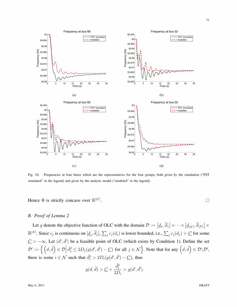
Figure 10 shows the frequencies at four of the 68 buses, which are representatives for the
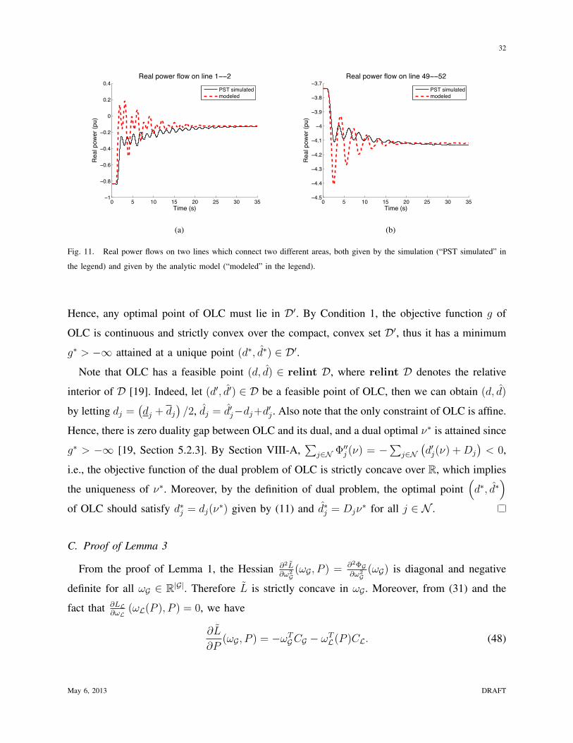
four groups, both given by the simulation and given by the analytic model. Figure 11 shows the
real power flows on two of the lines connecting two groups, both given by the simulation and
given by the analytic model. As we can see, the analytic model is a reasonable approximation
of the more realistic simulation model.
May 6, 2013 DRAFT
30
0 10 20 30 40 5059.955
59.96
59.965
59.97
59.975
59.98
59.985
59.99
59.995
60
60.005Frequency at group 1
Time (s)
Freq
uenc
y (H
z)
(a)
0 10 20 30 40 5059.94
59.95
59.96
59.97
59.98
59.99
60
60.01
60.02Frequency at group 2
Time (s)
Freq
uenc
y (H
z)
(b)
0 10 20 30 40 5059.95
59.955
59.96
59.965
59.97
59.975
59.98
59.985
59.99
59.995
60Frequency at group 3
Time (s)
Freq
uenc
y (H
z)
(c)
0 10 20 30 40 5059.955
59.96
59.965
59.97
59.975
59.98
59.985
59.99
59.995
60
60.005Frequency at group 4
Time (s)
Freq
uenc
y (H
z)
(d)
Fig. 9. Bus frequencies in each of the four groups.
VIII. APPENDIX: PROOFS
A. Proof of Lemma 1
From (11), either c0j
(d
j
(⌫)) = ⌫ or d0j
(⌫) = 0. Hence, in (10) we haved
d⌫
(c
j
(d
j
(⌫))� ⌫d
j
(⌫)) = c
0j
(d
j
(⌫))d
0j
(⌫)� d
j
(⌫)� ⌫d
0j
(⌫) = �d
j
(⌫),
and thus@�
@⌫
j
(⌫) = �
0j
(⌫
j
) = �d
j
(⌫
j
)�D
j
⌫
j
+ P
m
j
.
Hence the Hessian of � is diagonal. Moreover, since d
j
(⌫
j
) given by (11) is nondecreasing in
⌫
j
, we have@
2�
@⌫
2j
(⌫) = �
00j
(⌫
j
) = �d
0j
(⌫
j
)�D
j
< 0.
May 6, 2013 DRAFT
31
0 5 10 15 20 25 30 3559.96
59.965
59.97
59.975
59.98
59.985
59.99
59.995
60
Time (s)
Freq
uenc
y (H
z)
Frequency at bus 66
PST simulatedmodeled
(a)
0 5 10 15 20 25 30 3559.955
59.96
59.965
59.97
59.975
59.98
59.985
59.99
59.995
60
60.005
Time (s)
Freq
uenc
y (H
z)
Frequency at bus 53
PST simulatedmodeled
(b)
0 5 10 15 20 25 30 3559.955
59.96
59.965
59.97
59.975
59.98
59.985
59.99
59.995
60
60.005
Time (s)
Freq
uenc
y (H
z)
Frequency at bus 65
PST simulatedmodeled
(c)
0 5 10 15 20 25 30 3559.96
59.965
59.97
59.975
59.98
59.985
59.99
59.995
60
Time (s)
Freq
uenc
y (H
z)
Frequency at bus 50
PST simulatedmodeled
(d)
Fig. 10. Frequencies at four buses which are the representatives for the four groups, both given by the simulation (“PST
simulated” in the legend) and given by the analytic model (“modeled” in the legend).
Hence � is strictly concave over R|N |.
B. Proof of Lemma 2
Let g denote the objective function of OLC with the domain D :=
⇥
d1, d1
⇤
⇥· · ·⇥⇥
d|N |, d|N |⇤
⇥
R|N |. Since c
j
is continuous on [d
j
, d
j
],P
j
c
j
(d
j
) is lower bounded, i.e.,P
j
c
j
(d
j
) > C for some
C > �1. Let (d0, ˆd0) be a feasible point of OLC (which exists by Condition 1). Define the set
D0:=
n⇣
d,
ˆ
d
⌘
2 D�
�
�
ˆ
d
2j
2D
j
(g(d
0,
ˆ
d
0)� C) for all j 2 N
o
. Note that for any⇣
d,
ˆ
d
⌘
2 D\D0,
there is some i 2 N such that ˆ
d
2i
> 2D
i
(g(d
0,
ˆ
d
0)� C), thus
g(d,
ˆ
d) > C +
ˆ
d
2i
2D
i
> g(d
0,
ˆ
d
0).
May 6, 2013 DRAFT
32
0 5 10 15 20 25 30 35−1
−0.8
−0.6
−0.4
−0.2
0
0.2
0.4Real power flow on line 1−−2
Time (s)
Rea
l pow
er (p
u)
PST simulatedmodeled
(a)
0 5 10 15 20 25 30 35−4.5
−4.4
−4.3
−4.2
−4.1
−4
−3.9
−3.8
−3.7Real power flow on line 49−−52
Time (s)
Rea
l pow
er (p
u)
PST simulatedmodeled
(b)
Fig. 11. Real power flows on two lines which connect two different areas, both given by the simulation (“PST simulated” in
the legend) and given by the analytic model (“modeled” in the legend).
Hence, any optimal point of OLC must lie in D0. By Condition 1, the objective function g of
OLC is continuous and strictly convex over the compact, convex set D0, thus it has a minimum
g
⇤> �1 attained at a unique point (d⇤, ˆd⇤) 2 D0.
Note that OLC has a feasible point (d, ˆd) 2 relint D, where relint D denotes the relative
interior of D [19]. Indeed, let (d0, ˆd0) 2 D be a feasible point of OLC, then we can obtain (d,
ˆ
d)
by letting d
j
=
�
d
j
+ d
j
�
/2, ˆdj
=
ˆ
d
0j
�d
j
+d
0j
. Also note that the only constraint of OLC is affine.
Hence, there is zero duality gap between OLC and its dual, and a dual optimal ⌫⇤ is attained since
g
⇤> �1 [19, Section 5.2.3]. By Section VIII-A,
P
j2N �
00j
(⌫) = �P
j2N�
d
0j
(⌫) +D
j
�
< 0,
i.e., the objective function of the dual problem of OLC is strictly concave over R, which implies
the uniqueness of ⌫
⇤. Moreover, by the definition of dual problem, the optimal point⇣
d
⇤,
ˆ
d
⇤⌘
of OLC should satisfy d
⇤j
= d
j
(⌫
⇤) given by (11) and ˆ
d
⇤j
= D
j
⌫
⇤ for all j 2 N .
C. Proof of Lemma 3
From the proof of Lemma 1, the Hessian @
2L
@!
2G(!G, P ) =
@
2�G@!
2G(!G) is diagonal and negative
definite for all !G 2 R|G|. Therefore ˜
L is strictly concave in !G . Moreover, from (31) and the
fact that @LL@!L
(!L(P ), P ) = 0, we have
@
˜
L
@P
(!G, P ) = �!
T
GCG � !
T
L(P )CL. (48)
May 6, 2013 DRAFT
33
Therefore we have (using (30))@
2˜
L
@P
2(!G, P ) = �C
T
L@!L
@P
(P ) = �C
T
L
✓
@
2�L
@!
2L
(!L(P ))
◆�1
CL.
From the proof of Lemma 1, @
2�L@!
2L
is diagonal and negative definite. Hence @
2L
@P
2 (!G, P ) is positive
semidefinite and ˜
L is convex in P (˜L may not be strictly convex in P because CL is not
necessarily of full rank).
D. Proof of Lemma 4
The equivalence of (40) and (39) follows directly from the definition of !L(P ). To prove that
(40) is necessary and sufficient for ˙
U(!, P ) = 0, we first claim that the discussion preceding
the lemma implies that (!, P ) = (!G,!L, P ) satisfies ˙
U(!, P ) = 0 if and only if
!G = !
⇤1G and
@
˜
L
@P
(!G, P ) (P � P
⇤) = 0. (49)
Indeed, if (49) holds, then the expression in (34) evaluates to zero. Conversely, if ˙
U(!, P ) = 0,
then the inequality in (35) must hold with equality, which is possible only if !G = !
⇤1G since ˜
L
is strictly concave in !G . Then we must have @L
@P
(!G, P ) (P � P
⇤) = 0 since the expression in
(34) needs to be zero. Hence we only need to establish the equivalence of (49) and (40). Indeed,
with !G = !
⇤1G , the other part of (49) becomes
@
˜
L
@P
(!
⇤1G, P ) (P � P
⇤) = �
⇥
!
⇤1
T
G !
T
L(P )
⇤
C(P � P
⇤) (50)
= �⇥
0 !
T
L(P )� !
⇤1
T
L⇤
C(P � P
⇤) (51)
= � (!L(P )� !
⇤1L)
T
CL(P � P
⇤)
= � (!L(P )� !
⇤1L)
T
@�L
@!L(!L(P ))� @�L
@!L(!
⇤1L)
�
T
, (52)
where (50) follows from (48), (51) follows from 1
T
N C = 0, and (52) follows from (23) and (26).
Note that �L is separable over !
j
for j 2 L and, from (10), �0j
(!
j
) = �d
j
(!
j
)�D
j
!
j
+ P
m
j
.
Writing DL := diag(Dj
, j 2 L), we hence have@
˜
L
@P
(!
⇤1G, P ) (P � P
⇤) = (!L(P )� !
⇤1L)
T
DL (!L(P )� !
⇤1L)
+
X
j2L
(!
j
(P )� !
⇤) (d
j
(!
j
(P ))� d
j
(!
⇤)) . (53)
Since d
j
(!
j
) given by (11) is nondecreasing in !
j
, each term in the summation above is
nonnegative for all P . Hence (53) evaluates to zero if and only if !L(P ) = !
⇤1L, establishing
the equivalence of (49) and (40).
May 6, 2013 DRAFT
34
E. Proof of Lemma 5
The proof of LaSalle’s invariance principle in [26, Theorem 3.4] shows that (!(t), P (t))
approaches its positive limit set Z
+ which is nonempty, compact, invariant, and a subset of
E, as t ! 1. It is sufficient to show that Z
+ ✓ Z
⇤, i.e., considering any point (!, P ) =
(!G,!L, P ) 2 Z
+, to show that (!, P ) 2 Z
⇤. By (28), (41) and the fact that (!, P ) 2 E, we
only need to show that
CGP =
@�G
@!G(!G)
�
T
. (54)
Since Z
+ is invariant with respect to (22)–(24), a trajectory (!(t), P (t)) that starts in Z
+ must
stay in Z
+, and hence stay in E. By (41), !G(t) = !
⇤1G for all t � 0, and therefore !G(t) = 0
for all t � 0. Hence, by (22), any trajectory (!(t), P (t)) in Z
+ should satisfy
CGP (t) =
@�G
@!G(!G(t))
�
T
for all t � 0, which implies that (54) holds for any (!, P ) 2 Z
+.
REFERENCES
[1] A. J. Wood and B. F. Wollenberg, Power Generation, Operation, and Control, 2nd Edition. NJ: John Wiley & Sons, Inc.,
1996.
[2] A. R. Bergen and V. Vittal, Power Systems Analysis, 2nd ed. Upper Saddle River, NJ: Prentice Hall, 2000.
[3] G. Rogers. Power System Oscillations. MA, US: Kluwer Academic Publishers, 2000.
[4] G. Heffner, C. Goldman, B. Kirby and M. Kintner-Meyer, “Loads providing ancillary services: Review of international
experience,” Technical Report, Lawrence Berkeley National Laboratory, LBNL-62701, May 2007.
[5] A. Brooks, E. Liu, D. Reicher, C. Spirakis and B. Weihl, “Demand dispatch: Using real-time control of demand to help
balance generation and load,” IEEE Power&Energy Magazine, vol. 8, no. 3, pp. 21-30, 2010.
[6] B. Kirby, “Spinning Reserve From Responsive Loads,” Technical Report, Oak Ridge National Laboratory, ORNL/TM-
2003/19, March 2003.
[7] A. Molina-Garcia, F. Bouffard and D. S. Kirschen, “Decentralized demand-side contribution to primary frequency control,”
IEEE Transactions on Power Systems, vol. 26, no. 1, pp. 411-419, 2001.
[8] M. Donnelly, D. Harvey, R. Munson and D. Trudnowski, “Frequency and stability control using decentralized intelligent
loads: Benefits and pitfalls,” in Proc. of the IEEE Power and Energy Society General Meeting, Minneapolis, MN, USA,
2010.
[9] C. Zhao, U. Topcu, S. Low, “Frequency-based load control in power systems,” in Proc. of American Control Conference,
Montreal, Quebec, Canada, June 2012.
[10] C. Zhao, U. Topcu, S. Low, “Fast load control with stochastic frequency measurement,” in Proc. of the IEEE Power and
Energy Society General Meeting, San Diego, CA, USA, July 2012.
May 6, 2013 DRAFT
35
[11] C. Zhao, U. Topcu, S. Low, “Optimal load control via frequency measurement and neighborhood area communication,”
IEEE Transactions on Power Systems, 2013.
[12] J. Chow and G. Rogers, Power System Toolbox, Version 3.0, 1991-2008.
[13] M. D. Ilic, L. Xie, U. A. Khan, J. M. F. Moura, “Modeling of future cyberphysical energy systems for distributed sensing
and control,” IEEE Transactions on Systems, Man, and Cybernetics – Part A: Systems and Humans, vol. 40, no. 4, pp.
825-838, 2010.
[14] M. Ilic and Q. Liu, “Toward sensing, communications and control architectures for frequency regulation in systems with
highly variable resources,” Control and Optimization Theory for Electric Smart Grids. New York: Springer, 2012.
[15] M. Fahrioglu, F. L. Alvarado, “Designing incentive compatible contracts for effective demand management,” IEEE
Transactions on Power Systems, vol. 15, no. 4, pp. 1255-1260, 2000.
[16] P. Samadi, A. Mohsenian-Rad, R. Schober, V. W. S. Wong, J. Jatskevich, “Optimal Real-time pricing algorithm based on
utility maximization for smart grid,” Proc. of the IEEE SmartGridComm, Brussels, Belgium, October 2011.
[17] B. Ramanathan, V. Vittal, “A framework for evaluation of advanced direct load control with minimum disruption,” IEEE
Transactions on Power Systems, vol. 23, no. 4, pp. 1681-1688, 2008.
[18] Z. Ma, D. Callaway, I. Hiskens, “Decentralized charging control for large populations of plug-in vehicles: application
of the Nash certainty equivalence principle,” Proc. of IEEE Multi-Conference on Systems and Control, Yokohama, Japan,
September 2010.
[19] S. Boyd and L. Vandenberghe, Convex Optimization, UK: Cambridge University Press, 2004.
[20] W. Rudin, Principles of Mathematical Analysis, 3rd ed. New York: McGraw-Hill Book Co., 1976. pp.
[21] P. V. Mieghem, Graph Spectra for Complex Networks. UK: Cambridge University Press, 2011.
[22] K. Arrow, L. Hurwicz and H. Uzawa, Studies in Linear and Non-Linear Programming. CA, US: Stanford University Press,
1958.
[23] A. Rantzer, “Dynamic dual decomposition for distributed control,” in Proc. of American Control Conference, St. Louis,
MO, USA, June 2009.
[24] D. Feijer and F. Paganini, “Stability of primal-dual gradient dynamics and applications to network optimization,”
Automatica, vol. 46, no. 12, 2010, pp. 1974-1981.
[25] P. J. Douglass, R. Garcia-Valle, P. Nyeng, J. Ostergaard and M. Togeby, “Smart demand for frequency regulation:
Experimental results,” IEEE Transactions on Smart Grid, 2012.
[26] H. K. Khalil, Nonlinear Systems, 2nd ed. NJ, US: Prentice-Hall, Inc., 1996.
May 6, 2013 DRAFT