1

Practical aspects of GWASAssociation studies under statistical genetics

and GenABEL hands-on tutorial

2

Table of contents

• Introduction to genetic statistical analysis in GWA– Typical study designs / general idea– Popular genetic models of inheritance– Regression-based models in context of GWA

• GenABEL tutorial on GWAS case-control study– Main library features and how access them– Data filtering and QC– Accounting for population stratification

3

The main question of GWA studies• What is the causal model underlying genetic association?

Source: Ziegler and Van Steen 2010

4

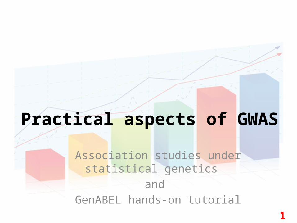
Important genetic terms• Given position in the genome (i.e. locus) has several

associated alleles (A and G) which produce genotypes rA/rG

• Haplotypes– Combination of alleles at different loci

5

Genotype coding

• For given bi-allelic marker/SNP/loci there could be total of 3 possible genotypes given alleles A and a

Note: A is major allele and a is minor

Genotype CodingAA 0Aa 1aa 2

6

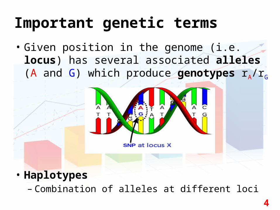
Stats Review: Multiplication Rule

• Only valid for independent events (e.g. A and B)

P(A and B) = P(A) * P(B)

Table of probabilities of events A and B

• P(A) = 0.20, P(B) = 0.70, A and B are independent• P(A and B) = 0.20 * 0.70 = 0.14

B B' (not B) MarginalA 0.14 0.06 0.2

A' (not A) 0.56 0.24 0.8Marginal 0.7 0.3 1

7

Stats review: Chi square test

• Tests if there is a difference between two normal distributions (e.g. observed vs theoretical)– Hypothesis based test– Pearson's chi-squared test of independence (default)

Ho: null hypothesis stating that markers have no association to the trait (e.g. disease state)Ha: alternative hypothesis there is non-random association

8

X2 test - hypothetical example • Given data on individuals, determine if there is

association between smoking and disease?

• X2 = 105[(36)(25) - (14)(30)]2 / (50)(55)(39)(66)• X2 = 3.4178 p-value = 0.065 @ df=1• Conclusion: no statistical significant link at α=0.05

(p<0.05) between smoking and disease occurrence

Smoker Non-smoker TotalCases 36(a) 14 (b) 50 (a+b)Controls 30(c) 25 (d) 55 (c+d) Total 66 (a+c) 39 (b+d) 105 (N)

2( )2( )(c d)(b d)(a c)

ad bcX Na b

9

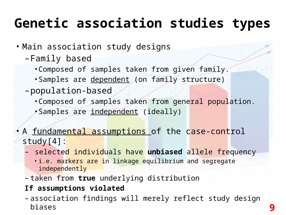
Genetic association studies types• Main association study designs

– Family based• Composed of samples taken from given family. • Samples are dependent (on family structure)

– population-based• Composed of samples taken from general population.• Samples are independent (ideally)

• A fundamental assumptions of the case-control study[4]:– selected individuals have unbiased allele frequency

• i.e. markers are in linkage equilibrium and segregate independently

– taken from true underlying distribution If assumptions violated– association findings will merely reflect study design biases

10

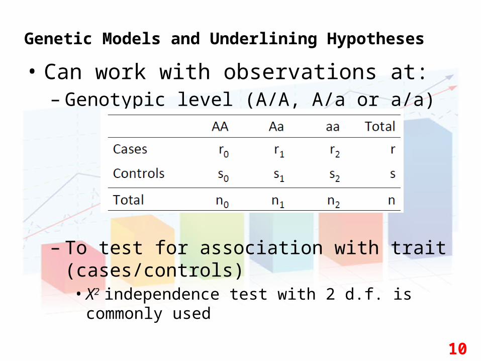
Genetic Models and Underlining Hypotheses• Can work with observations at:

– Genotypic level (A/A, A/a or a/a)

– To test for association with trait (cases/controls)• X2 independence test with 2 d.f. is commonly used

11

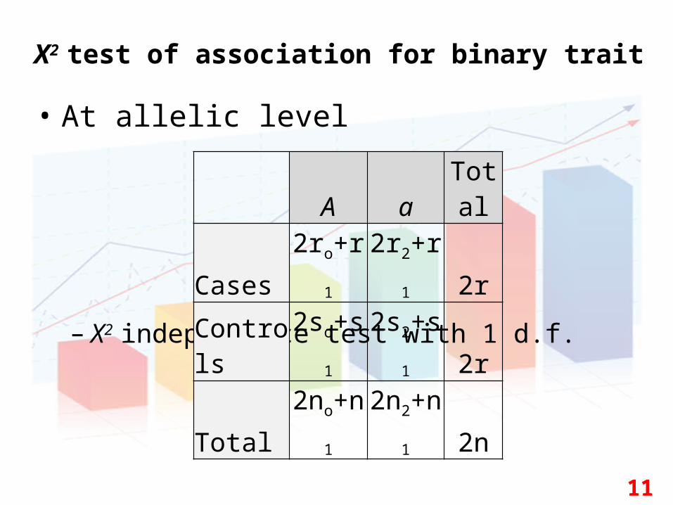
X2 test of association for binary trait

• At allelic level

– X2 independence test with 1 d.f.

A a TotalCases 2ro+r1 2r2+r1 2rControls 2so+s1 2s2+s1 2rTotal 2no+n1 2n2+n1 2n

12

Trait inheritance• Allelic penetrance - the proportion of individuals in a

population who carry a disease-causing allele and express the disease phenotype [5]– Trait T: coded phenotype – Penetrance: P(T|Genotype)– Complete penetrance: P(T|G) = 1

• Mendelian inheritance – traits that follow Mendelian Laws of inheritance from parents to children (e.g. eye/hair color)– alleles of different genes separate independently of one another

when sex cells/gametes are formed– not all traits follow these laws (allele conversion, epigenetics)

13

Genetic allelic dominance

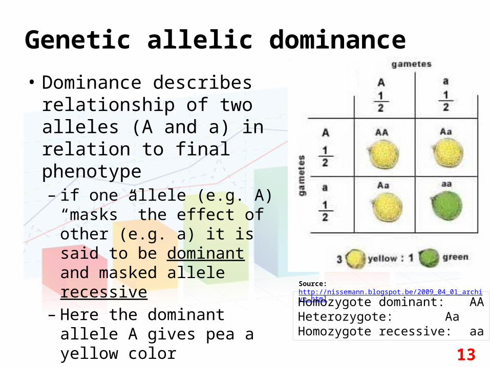
• Dominance describes relationship of two alleles (A and a) in relation to final phenotype– if one allele (e.g. A)

“masks” the effect of other (e.g. a) it is said to be dominant and masked allele recessive

– Here the dominant allele A gives pea a yellow color

Source: http://nissemann.blogspot.be/2009_04_01_archive.html

Homozygote dominant: AAHeterozygote: AaHomozygote recessive: aa

14

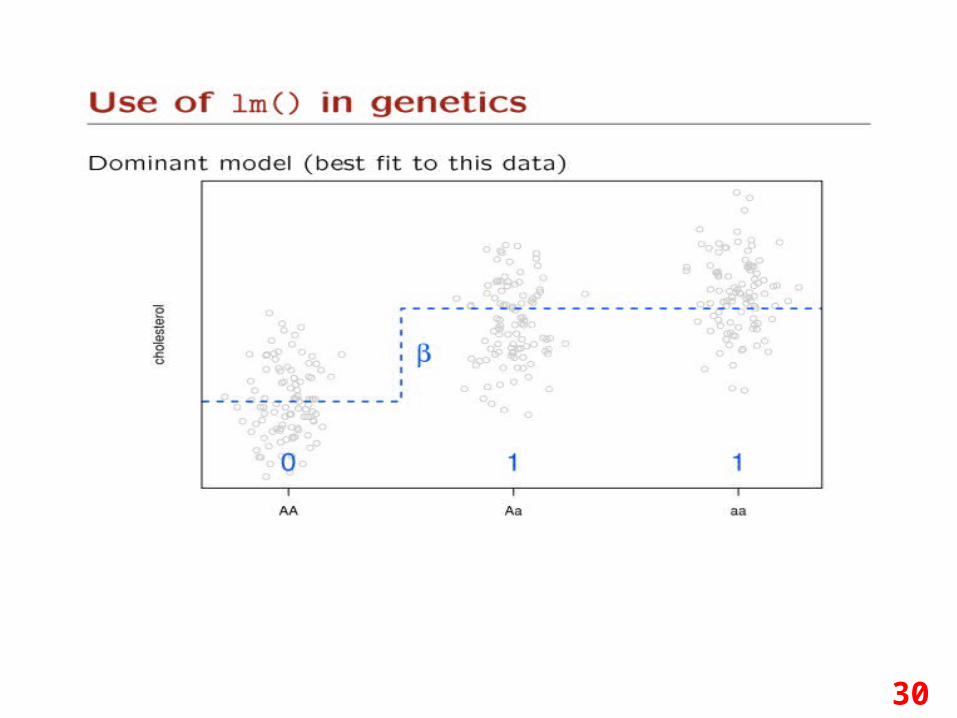
Genotype genetic based models

Dominant

Heterozygous

Recessive

• Hypothesis (Ho): the genetic effects of AA and Aa are the same (A is dominant allele)• Hypothesis (Ho): the genetic effects of aa and AA are the same• Hypothesis (Ho): the genetic effects of aa and Aa are the same (a is recessive allele)

15

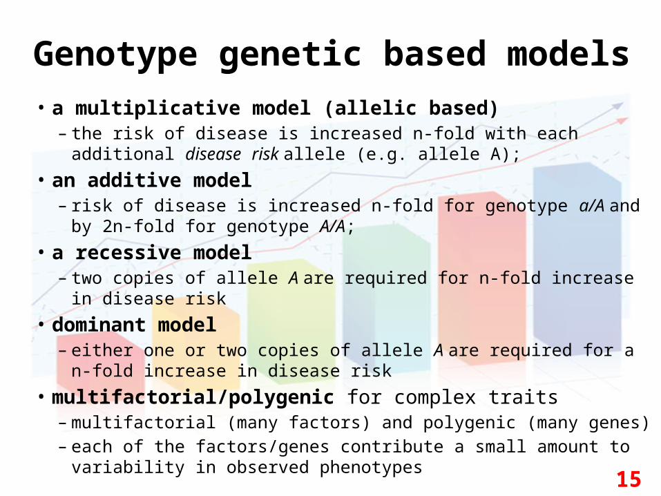
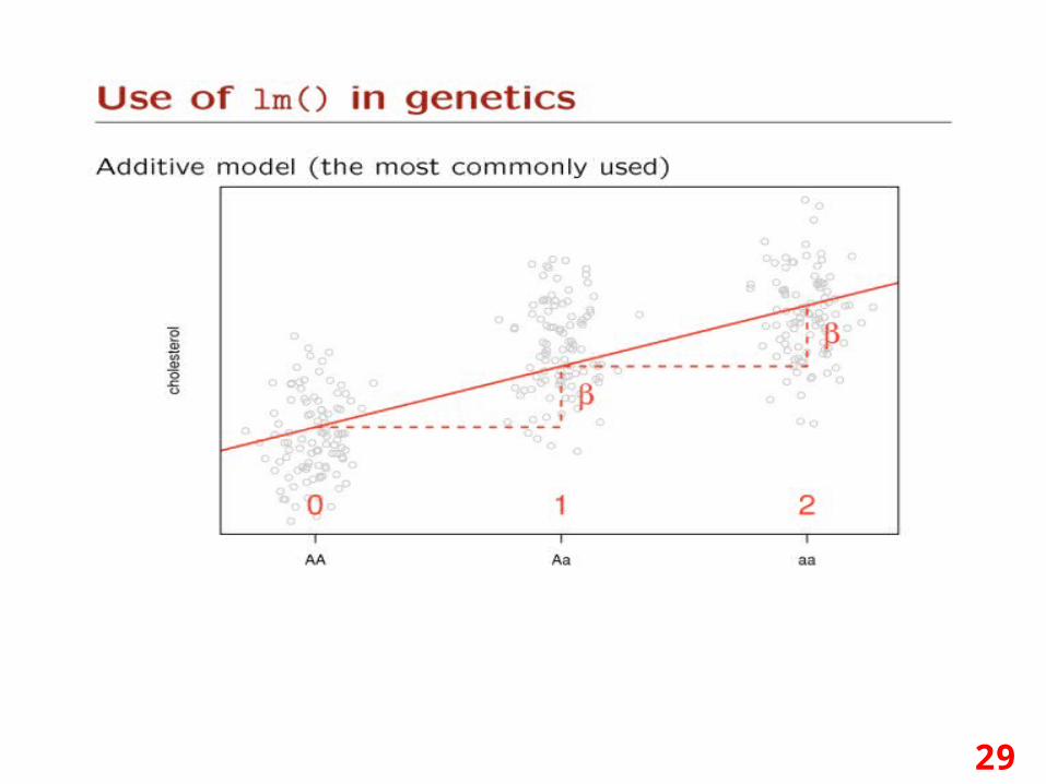
Genotype genetic based models• a multiplicative model (allelic based)

– the risk of disease is increased n-fold with each additional disease risk allele (e.g. allele A);

• an additive model– risk of disease is increased n-fold for genotype a/A and by 2n-fold for

genotype A/A; • a recessive model

– two copies of allele A are required for n-fold increase in disease risk• dominant model

– either one or two copies of allele A are required for a n-fold increase in disease risk

• multifactorial/polygenic for complex traits– multifactorial (many factors) and polygenic (many genes)– each of the factors/genes contribute a small amount to variability in

observed phenotypes

16

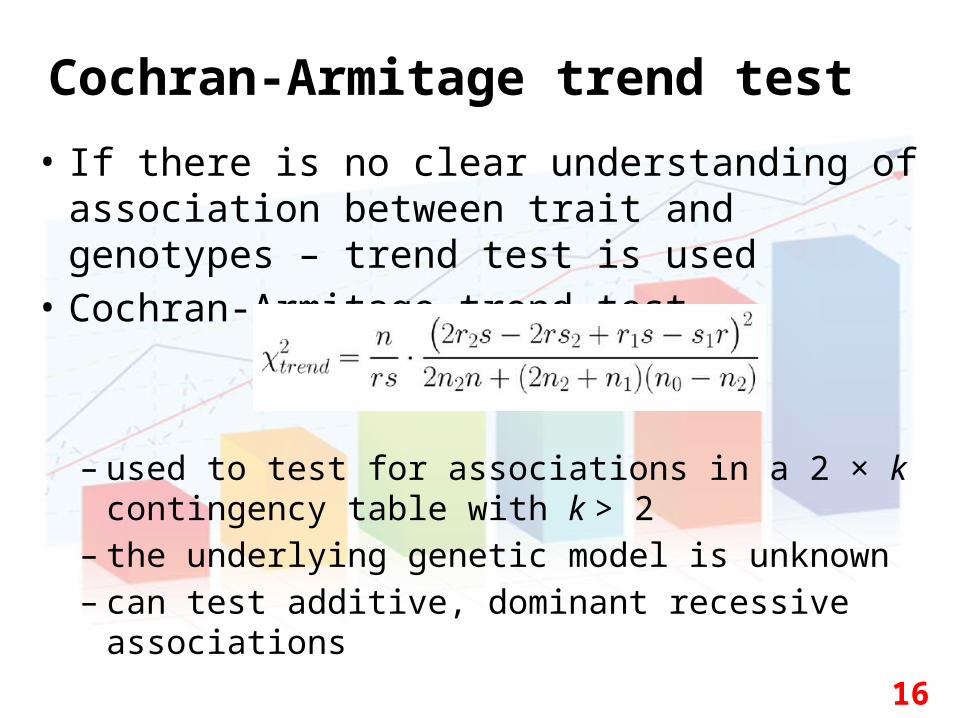
Cochran-Armitage trend test

• If there is no clear understanding of association between trait and genotypes – trend test is used

• Cochran-Armitage trend test

– used to test for associations in a 2 × k contingency table with k > 2

– the underlying genetic model is unknown– can test additive, dominant recessive associations

17

Which test should be used?

• Depends to apriori knowledge and dataset• Trend test if no biological hypothesis exists

– Under additive model assumption trait test is identical allelic test if HWE criteria fulfilled

• Dominant model for dominant-based traits• Recessive model for recessive -based traits• At low minor allele frequencies (MAFs),

recessive tests have little power

18

Measurement of genetic effects on traits

• The relative risk (RR):

– Compares the disease penetrances between individuals with different genotypes at assayed loci

– should not know outcome a priori (before the experiment ends)

– In typical case-control study where the ratio of cases to controls is controlled, it is not possible to make direct estimates of disease penetrance and RRs

19

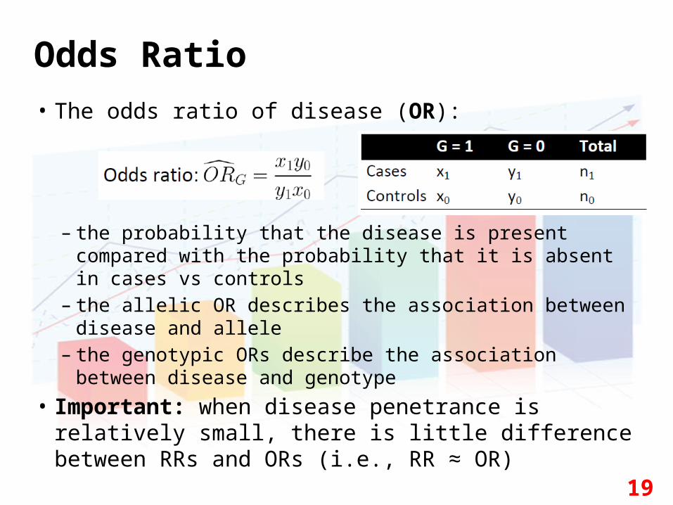
Odds Ratio• The odds ratio of disease (OR):

– the probability that the disease is present compared with the probability that it is absent in cases vs controls

– the allelic OR describes the association between disease and allele

– the genotypic ORs describe the association between disease and genotype

• Important: when disease penetrance is relatively small, there is little difference between RRs and ORs (i.e., RR ≈ OR)

20

OR illustration

• Histogram of estimated ORs (estimate of genetic effect size) at confirmed susceptibility loci

Source: Iles MM. What can genome-wide association studies tell us about the genetics of common disease? PLoS Genet. 2008 Feb;4(2):e33

21

Regression methods under statistical genomics context

22

Regression analysis

• Looks to explain relationship existing between single variable Y (the response, output or dependent variable) and one or more predictor, variables (input, independent or explanatory) X1, …, Xp (if p>1 multivariate regression)

• Advantages over correlation coefficient:– Gives measure of how model fits data (yfit)

– Can predict other variable values (e.g. intercept)

𝑦=𝑎+𝑏𝑥 response co-variate x

 A

𝑒𝑟𝑟𝑜𝑟 (𝑟𝑒𝑠𝑖𝑑𝑢𝑎𝑙)=𝑦− 𝑦 𝑓𝑖𝑡

23

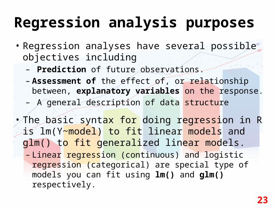
Regression analysis purposes• Regression analyses have several possible objectives

including – Prediction of future observations.– Assessment of the effect of, or relationship between,

explanatory variables on the response.– A general description of data structure

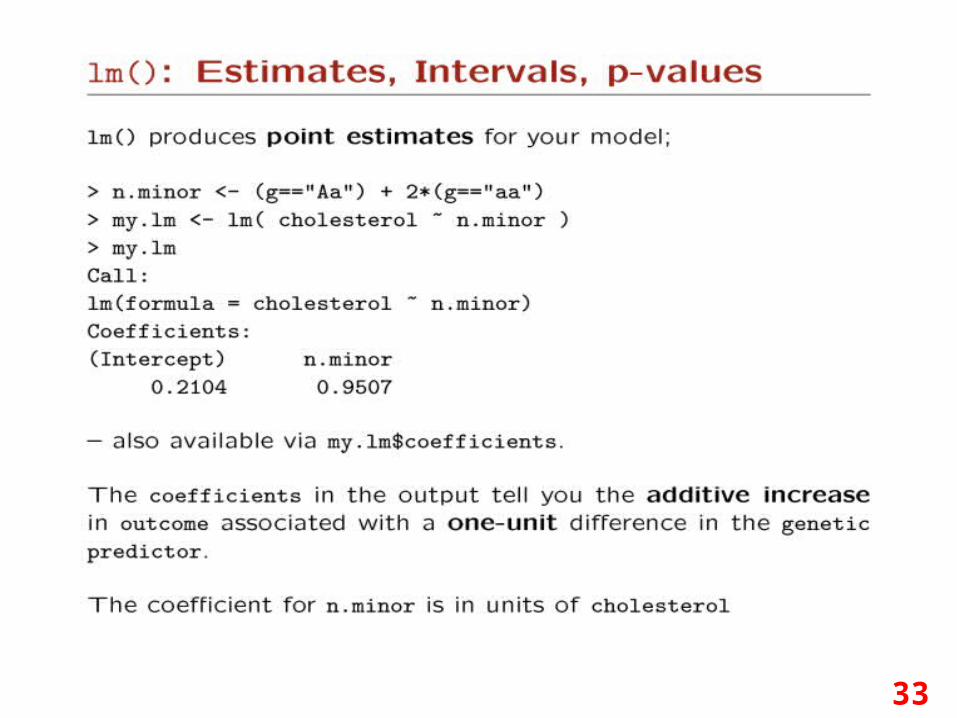
• The basic syntax for doing regression in R is lm(Y~model) to fit linear models and glm() to fit generalized linear models.– Linear regression (continuous) and logistic regression

(categorical) are special type of models you can fit using lm() and glm() respectively.

24

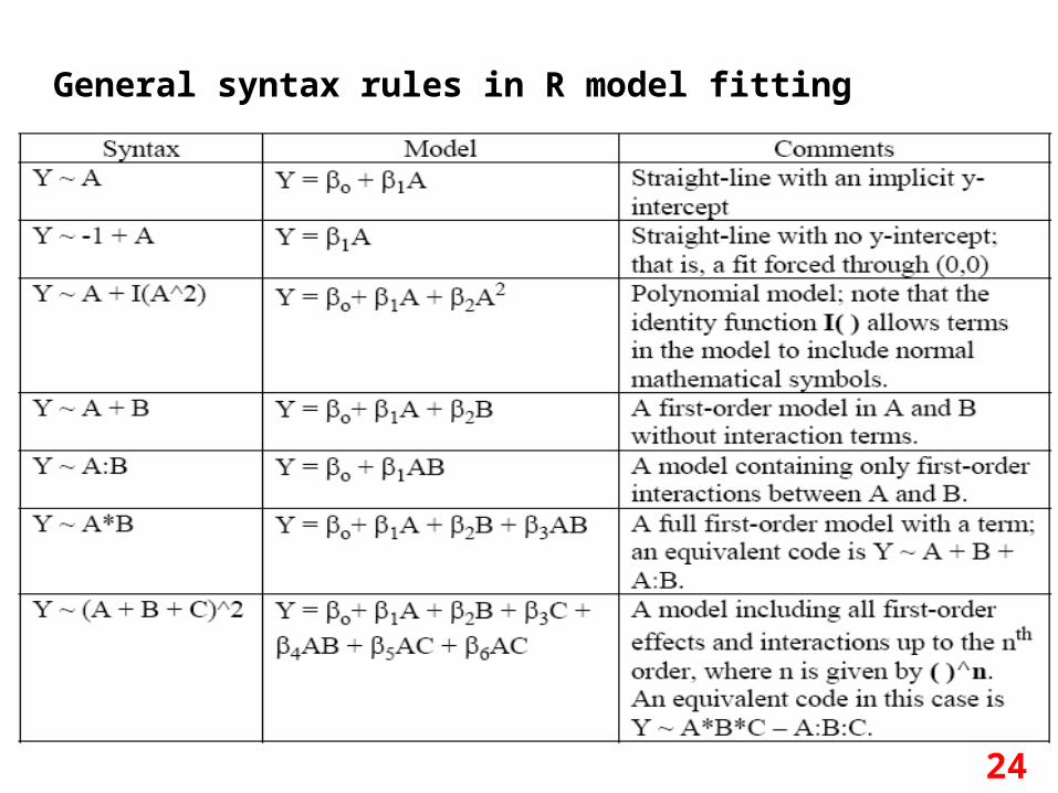
General syntax rules in R model fitting

25

Linear regression assumptions

• There are four principal assumptions which justify the use of linear regression models for purposes of prediction: – linearity of the relationship between dependent (y)

and independent variables (x)– independence of observations (not a time series) – homoscedasticity (constant variance) of the errors

• versus time (residuals getting larger with time)• versus the predictions

• normality of the error distribution – Detect skewness of errors (kurtosis test)

See http://www.duke.edu/~rnau/testing.htm

26

Linear regression – violation of linearity

• Violations of linearity are extremely serious--if you fit a linear model to data which are nonlinearly related– To detect

• plot of the observed versus predicted values or a plot of residuals versus predicted values, which are a part of standard regression output. The points should be symmetrically distributed around a diagonal line in the former plot or a horizontal line in the residuals plot. Look carefully for evidence of a "bowed" pattern

– To fix this issue• nonlinear transformation to the dependent and/or independent

variables• adding another regressor which is a nonlinear function of one of

the other variables (e.g. x2)

27

Coefficient of determination r2

• The value r2 is a fraction between 0.0 and 1.0, and has no units. – value of 0.0 means no relationship (that is knowing

X does not help you predict Y)– value of 1.0, all points lie exactly on a straight line

with no scatter. Knowing X lets you predict Y perfectly.

28

29

30

31

32

33

34

35

36

37

GenABEL libraryA practical introduction to Genome Wide

Association Studies

1

38

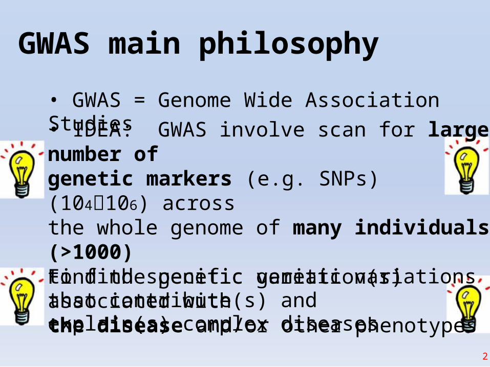
GWAS main philosophy

• GWAS = Genome Wide Association Studies• IDEA: GWAS involve scan for large number ofgenetic markers (e.g. SNPs) (104106) acrossthe whole genome of many individuals (>1000)to find specific genetic variations associated withthe disease and/or other phenotypesFind the genetic variation(s) that contribute(s) and explain(s) complex diseases

2

39

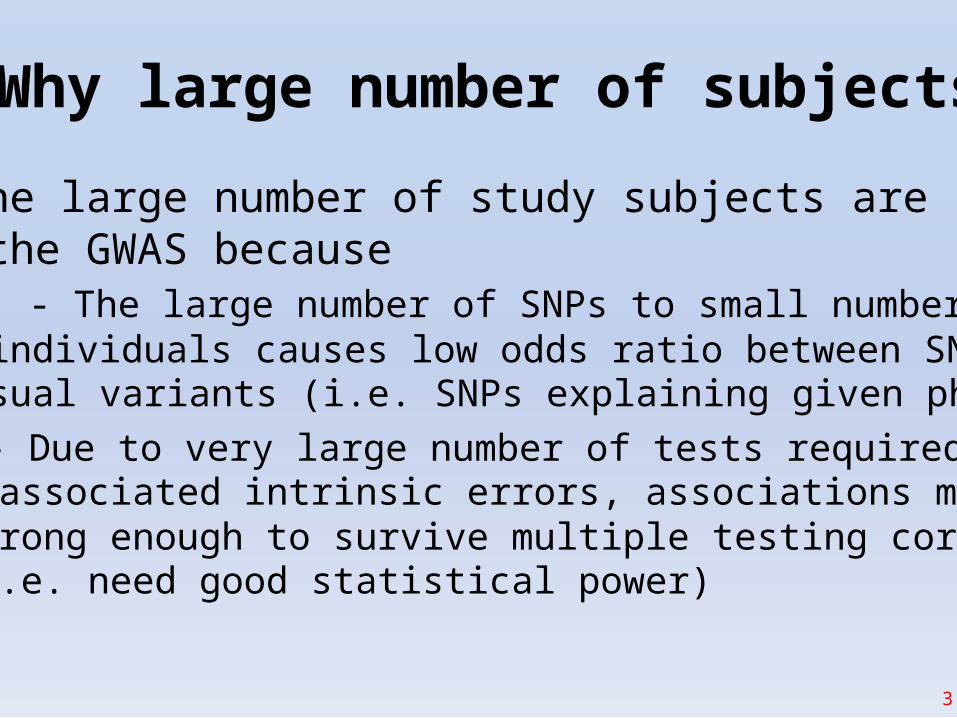
Why large number of subjects?

• The large number of study subjects are neededin the GWAS because

- The large number of SNPs to small number ofindividuals causes low odds ratio between SNPs and

casual variants (i.e. SNPs explaining given phenotype)- Due to very large number of tests required with

associated intrinsic errors, associations must bestrong enough to survive multiple testing corrections(i.e. need good statistical power)

3

40

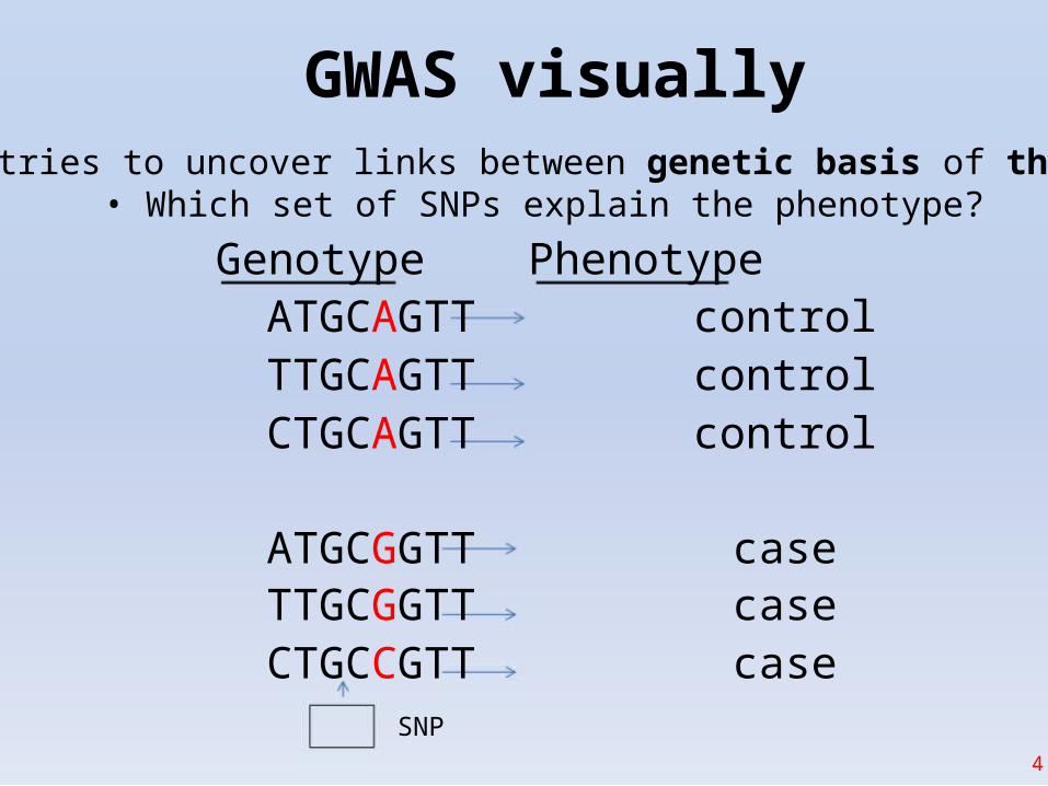
GWAS visually• GWAS tries to uncover links between genetic basis of the disease

• Which set of SNPs explain the phenotype?

Genotype PhenotypeATGCAGTTTTGCAGTTCTGCAGTT

ATGCGGTTTTGCGGTTCTGCCGTT

SNP

controlcontrolcontrol

casecasecase

4

41

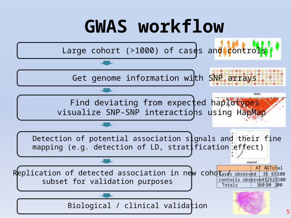
GWAS workflowLarge cohort (>1000) of cases and controls

Get genome information with SNP arrays

Find deviating from expected haplotypesvisualize SNP-SNP interactions using HapMap

Detection of potential association signals and their finemapping (e.g. detection of LD, stratification effect)

Replication of detected association in new cohot /subset for validation purposes

Biological / clinical validation

AT AGTotalcases observed 35 65 100contorls observed12525100Totals 160 90 200

5

42

Which tools to use to doGWAS workflows?

How to find SNP-Diseaseassociations?

6

43

Common tools

• Some of the popular tools- SVS Golden Helix (data filtering and normalization)

• Is commercial software providing ease of use compared toother free solutions requiring use of numerous libraries

• Has unique feature on CNV Analysis• Manual: http://doc.goldenhelix.com/SVS/latest/

- Biofilter (pre-selection of SNPs using database info)(http://ritchielab.psu.edu/ritchielab/software/)

- GenABEL library implemented in R (http://www.genabel.org/)

7

44

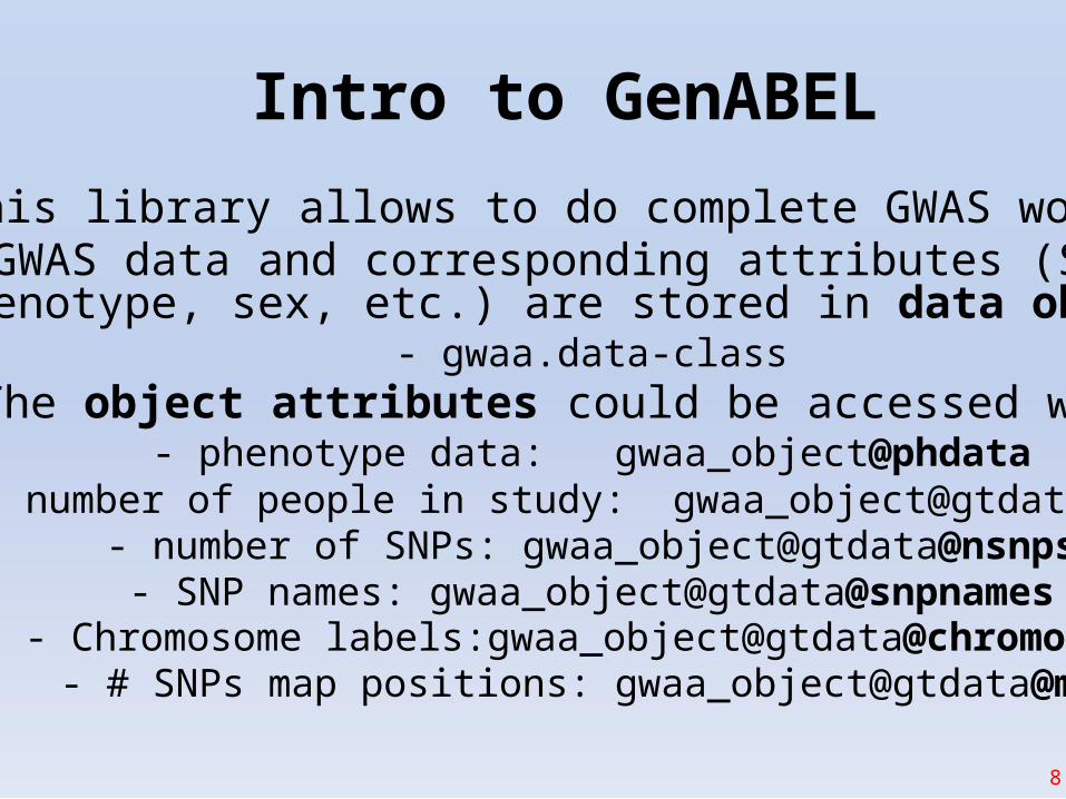
Intro to GenABEL

• This library allows to do complete GWAS workflow• GWAS data and corresponding attributes (SNPs,phenotype, sex, etc.) are stored in data object

- gwaa.data-class• The object attributes could be accessed with @

- phenotype data: gwaa_object@phdata- number of people in study: gwaa_object@gtdata@nids

- number of SNPs: gwaa_object@gtdata@nsnps- SNP names: gwaa_object@gtdata@snpnames

- Chromosome labels:gwaa_object@gtdata@chromosome- # SNPs map positions: gwaa_object@gtdata@map

8

45

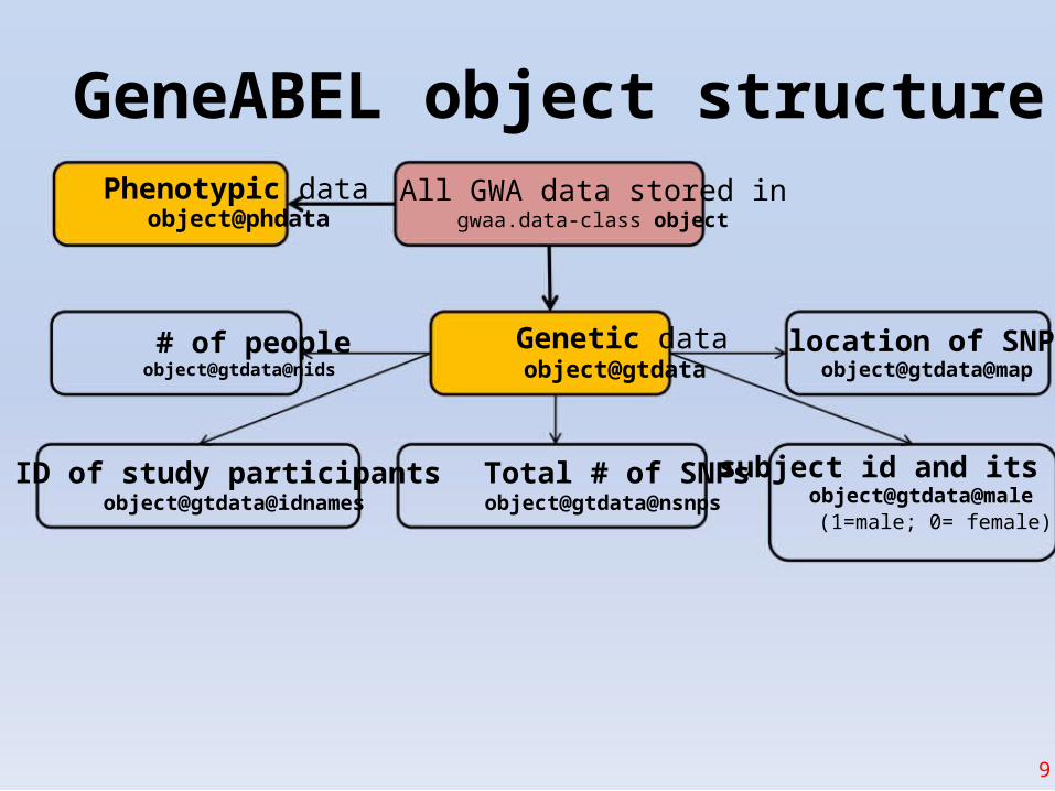
GeneABEL object structurePhenotypic data

object@phdata

# of peopleobject@gtdata@nids

ID of study participantsobject@gtdata@idnames

All GWA data stored ingwaa.data-class object

Genetic dataobject@gtdata

Total # of SNPsobject@gtdata@nsnps

location of SNPsobject@gtdata@map

subject id and its sexobject@gtdata@male

(1=male; 0= female)

9

46

Hands on GenABELinstall.packages("GenABEL")

library("GenABEL")data(ge03d2ex) #loads data(i.e. from GWAS) on type 2 diabetes

summary(ge03d2ex)[1:5,] #view first 5 SNP data (genotypic data)Chromosome Position Strand A1 A2 NoMeasured CallRate Q.2

rs1646456 1 653 + C G 135 0.9926471 0.33333333

rs4435802 1 5291 + C A 134 0.9852941 0.07462687

rs946364 1 8533 - T C 134 0.9852941 0.27611940

rs299251 1 10737 + A G 135 0.9926471 0.04444444

rs2456488 1 11779 + G C 135 0.9926471 0.34814815

>= 0,98 means good genotyping

summary(ge03d2ex@phdata) #view phenotypic dataid sex age dm2 height

Length:136 Min. :0.0000 Min. :23.84 Min. :0.0000 Min. :150.2Class :character 1st Qu.:0.0000 1st Qu.:38.33 1st Qu.:0.0000 1st Qu.:161.5Mode :character Median :1.0000 Median :48.71 Median :1.0000 Median :169.4

Mean :0.5294 Mean :49.07 Mean :0.6324 Mean :169.43rd Qu.:1.0000 3rd Qu.:58.57 3rd Qu.:1.0000 3rd Qu.:175.9Max. :1.0000 Max. :81.57 Max. :1.0000 Max. :191.8

NA's :1

P.11 P.12 P.22 Pexact Fmax Plrt57 66 12 0.3323747 -0.10000000 0.2404314

114 20 0 1.0000000 -0.08064516 0.2038385

68 58 8 0.3949055 -0.08275286 0.3302839

123 12 0 1.0000000 -0.04651163 0.4549295

59 58 18 0.5698988 0.05343327 0.5360019

weight diet bmiMin. : 46.63 Min. :0.00000 Min. :17.301st Qu.: 69.02 1st Qu.:0.00000 1st Qu.:24.56Median : 81.15 Median :0.00000 Median :28.35Mean : 87.40 Mean :0.05882 Mean :30.303rd Qu.:102.79 3rd Qu.:0.00000 3rd Qu.:35.69Max. :161.24 Max. :1.00000 Max. :59.83NA's :1 NA's :1

A1 A2 = allele 1 and 2 Position = genomic position (bp)Strand = DNA strand + or - CallRate = allelic frequency expressed as a ratio

NoMeasured = # of times the genotype was observedPexact = P-value of the exact test for HWE

Fmax = estimate of deviation from HWE, allowing meta-analysis10

47

Exploring phenotypic data• See aging phenotype data in compressed form

descriptives.trait(ge03d2ex)No Mean SD

id 136 NA NAsex 136 0.529 0.501age 136 49.069 12.926dm2 136 0.632 0.484height 135 169.440 9.814weight 135 87.397 25.510diet 136 0.059 0.236bmi 135 30.301 8.082

• Extract all sexes of all individualsge03d2ex@phdata$sex # accessing sex column of the data frame with $

1 0 1 0 0 1 1 0 0 1 0 0 1 1 0 0 0 1 1 1 1 1 1 1 1 1 1 0 1 0 1 0 1 1 0 0 0 1 1 1 1 0 1 11 0 1 1 1 1 0 1 1 1 1 0 1 0 1 0 0 1 0 1 1 0 1 0 0 1 0 1 1 1 1 1 0 1 0 0 1 0 1 0 0 0 0 00 0 0 1 0 0 0 1 1 0 1 1 0 1 0 1 0 1 1 0 0 0 0 1 0 1 0 0 0 1 0 0 1 0 0 1 1 0 1 1 1 0 1 0

0 1 1 0

• Sorting data by binary attribute (e.g. sex)descriptives.trait(ge03d2ex, by=ge03d2ex@phdata$sex)

No(by.var=0) Mean SD No(by.var=1)id 64 NA NAsex 64 NA NAage 64 46.942 12.479dm2 64 0.547 0.502height 64 162.680 6.819weight 64 78.605 26.908diet 64 0.109 0.315bmi 64 29.604 9.506

Mean SD Ptt Pkw Pexact72 NA NA NA NA NA72 NA NA NA NA NA72 50.959 13.107 0.070 0.081 NA72 0.708 0.458 0.053 0.052 0.07471 175.534 7.943 0.000 0.000 NA71 95.322 21.441 0.000 0.000 NA72 0.014 0.118 0.025 0.019 0.02671 30.930 6.547 0.352 0.040 NA

11Females Males

48

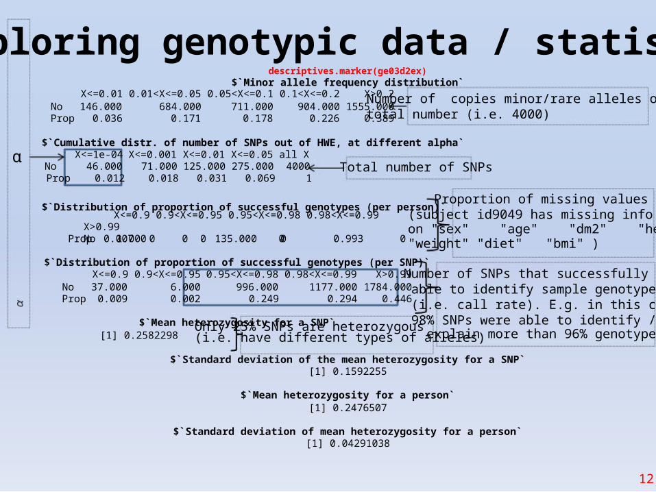
Exploring genotypic data / statisticsdescriptives.marker(ge03d2ex)

$`Minor allele frequency distribution`X<=0.01 0.01<X<=0.05 0.05<X<=0.1 0.1<X<=0.2 X>0.2

No 146.000 684.000 711.000 904.000 1555.000Prop 0.036 0.171 0.178 0.226 0.389

Number of copies minor/rare alleles out oftotal number (i.e. 4000)

$`Cumulative distr. of number of SNPs out of HWE, at different alpha`X<=1e-04 X<=0.001 X<=0.01 X<=0.05 all X

No 46.000 71.000 125.000 275.000 4000 Total number of SNPsProp 0.012 0.018 0.031 0.069 1

$`Distribution of proportion of successful genotypes (per person)`Proportion of missing values

X<=0.9 0.9<X<=0.95 0.95<X<=0.98 0.98<X<=0.99 X>0.99No 1.000 0 0 135.000 0Prop 0.007 0 0 0.993 0

$`Distribution of proportion of successful genotypes (per SNP)`X<=0.9 0.9<X<=0.95 0.95<X<=0.98 0.98<X<=0.99 X>0.99

No 37.000 6.000 996.000 1177.000 1784.000Prop 0.009 0.002 0.249 0.294 0.446

$`Mean heterozygosity for a SNP`

(subject id9049 has missing infoon "sex" "age" "dm2" "height""weight" "diet" "bmi" )

Number of SNPs that successfully wereable to identify sample genotype(i.e. call rate). E.g. in this case98% SNPs were able to identify /

[1] 0.2582298Only 25% SNPs are heterozygous(i.e. have different types of alleles)explain more than 96% genotypes

$`Standard deviation of the mean heterozygosity for a SNP`[1] 0.1592255

$`Mean heterozygosity for a person`[1] 0.2476507

$`Standard deviation of mean heterozygosity for a person`[1] 0.04291038

12

α

49

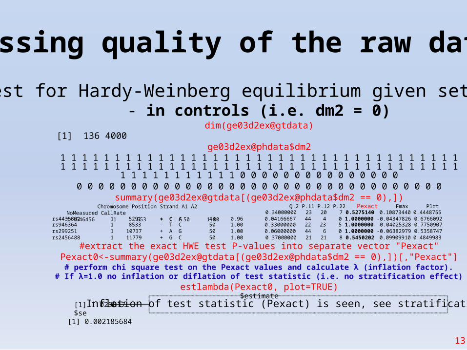
Assessing quality of the raw data (1)

1. Test for Hardy-Weinberg equilibrium given set of SNPs- in controls (i.e. dm2 = 0)

dim(ge03d2ex@gtdata)[1] 136 4000

ge03d2ex@phdata$dm21 1 1 1 1 1 1 1 1 1 1 1 1 1 1 1 1 1 1 1 1 1 1 1 1 1 1 1 1 1 1 1 1 1 1 1 11 1 1 1 1 1 1 1 1 1 1 1 1 1 1 1 1 1 1 1 1 1 1 1 1 1 1 1 1 1 1 1 1 1 1 1 1

1 1 1 1 1 1 1 1 1 1 1 0 0 0 0 0 0 0 0 0 0 0 0 0 0 00 0 0 0 0 0 0 0 0 0 0 0 0 0 0 0 0 0 0 0 0 0 0 0 0 0 0 0 0 0 0 0 0 0

summary(ge03d2ex@gtdata[(ge03d2ex@phdata$dm2 == 0),])Chromosome Position Strand A1 A2 NoMeasured CallRate

rs1646456 1 653 + C G 50 1.00rs4435802 1 5291 + C A 48 0.96rs946364 1 8533 - T C 50 1.00rs299251 1 10737 + A G 50 1.00rs2456488 1 11779 + G C 50 1.00

Q.2 P.11 P.12 P.22 Pexact Fmax Plrt0.34000000 23 20 7 0.5275140 0.10873440 0.44487550.04166667 44 4 0 1.0000000 -0.04347826 0.67660920.33000000 22 23 5 1.0000000 -0.04025328 0.77509070.06000000 44 6 0 1.0000000 -0.06382979 0.53587470.37000000 21 21 8 0.5450202 0.09909910 0.4849983

#extract the exact HWE test P-values into separate vector "Pexact"Pexact0<-summary(ge03d2ex@gtdata[(ge03d2ex@phdata$dm2 == 0),])[,"Pexact"]

# perform chi square test on the Pexact values and calculate λ (inflation factor).# If λ=1.0 no inflation or diflation of test statistic (i.e. no stratification effect)

estlambda(Pexact0, plot=TRUE)$estimate

[1] 1.029817$se

[1] 0.002185684

Inflation of test statistic (Pexact) is seen, see stratification effect

13

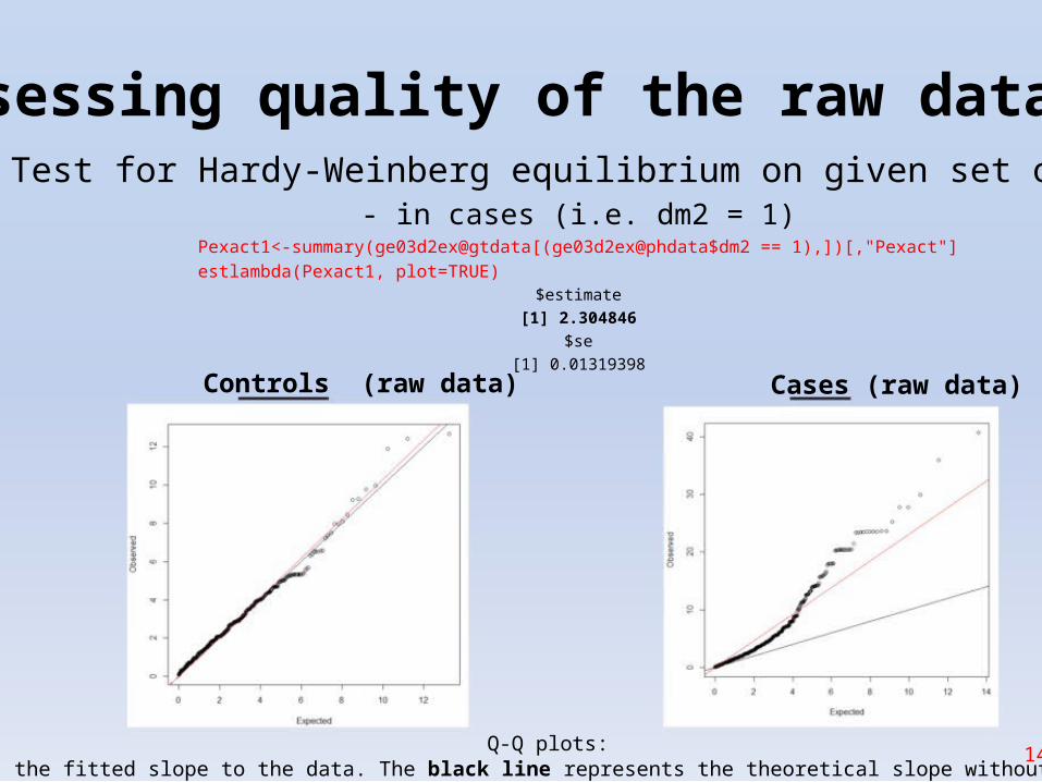
50

Assessing quality of the raw data (2)1. Test for Hardy-Weinberg equilibrium on given set of SNPs

- in cases (i.e. dm2 = 1)Pexact1<-summary(ge03d2ex@gtdata[(ge03d2ex@phdata$dm2 == 1),])[,"Pexact"]

estlambda(Pexact1, plot=TRUE)$estimate

[1] 2.304846$se

[1] 0.01319398Controls (raw data) Cases (raw data)

Q-Q plots: 14The red line shows the fitted slope to the data. The black line represents the theoretical slope without any stratification

51

A Fast and Simple Method For Genomewide Pedigree-Based Quantitative Trait - Loci Association Analysis

• Let’s apply a simple method that uses both mixedmodel and regression to find statistically significantassociations between trait (presence/absence ofdiabetes type 2) and loci (SNPs)qTest = qtscore(dm2,ge03d2ex,trait="binomial")

descriptives.scan(qTest, sort="Pc1df")Chromosome Position Strand A1 A2 N effB se_effB chi2.1df P1df effAB effBB chi2.2df P2df Pc1df

rs1719133 1 4495479 + T A 136 0.33729339 0.09282784 13.202591 0.0002795623 0.4004237 0.000000 14.729116 0.0006333052 0.0003504258

rs2975760 3 10518480 + A T 134 3.80380024 1.05172986 13.080580 0.0002983731 3.4545455 10.000000 13.547345 0.0011434877 0.0003732694rs7418878 1 2808520 + A T 136 3.08123060 0.93431795 10.875745 0.0009743183 3.6051282 4.871795 12.181064 0.0022642036 0.0011762545

rs5308595 3 10543128 - C G 133 3.98254950 1.21582875 10.729452 0.0010544366 3.3171429 Inf 10.766439 0.0045930101 0.0012699705rs4804634 1 2807417 + C G 132 0.43411456 0.13400290 10.494949 0.0011970132 0.5240642 0.173913 11.200767 0.0036964462 0.0014362332

effAB / effBB = odds ratio of each possible genotype combinationP1df / P2df = probability values from GWA analysis

Pc1df = probability values corrected for inflation factor (stratification effects) at 1 degree of freedom

# plot the lambda corrected values and visualize the Manhattan plotplot(qTest, df="Pc1df")

15

52

Manhattan plot of raw data

• To visualize to SNPs associated to the trait usedescriptives.scan(qTest)

• To see all the results covering all SNPsresults(qTest)

53

Empirical resembling with qtscore

• The previous GWA ran only once• Lets re-run 500 times the same test with randomresembling of the data

- This method is more rigorous- Empirical distribution of P-values are obtained

qTest.E <- qtscore(dm2,ge03d2ex,times=500)descriptives.scan(qTest.E,sort="Pc1df")

Chromosome Position Strand A1 A2 N effB se_effB chi2.1df P1df Pc1df effAB effBB chi2.2df P2dfrs1719133 1 4495479 + T A 136 -0.2652064 0.07298850 13.202591 0.458 0.540 -0.2080882 -0.7375000 14.729116 NArs2975760 3 10518480 + A T 134 0.2340655 0.06471782 13.080580 0.478 0.558 0.2755102 0.4090909 13.547345 NArs7418878 1 2808520 + A T 136 0.2089098 0.06334746 10.875745 0.862 0.912 0.2807405 0.3268398 12.181064 NArs5308595 3 10543128 - C G 133 0.2445516 0.07465893 10.729452 0.890 0.924 0.2564832 0.4623656 10.766439 NA

• None of the top SNPs hits the P<0.05 significance!• None of the "P2df" values pass threshold (i.e. all = NA)

17

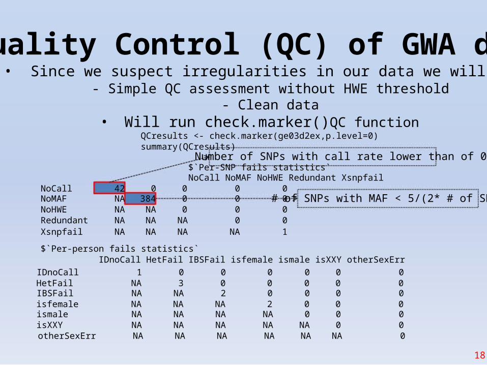
54

Quality Control (QC) of GWA data• Since we suspect irregularities in our data we will do

- Simple QC assessment without HWE threshold- Clean data

• Will run check.marker()QC functionQCresults <- check.marker(ge03d2ex,p.level=0)summary(QCresults)

Number of SNPs with call rate lower than of 0.95$`Per-SNP fails statistics`NoCall NoMAF NoHWE Redundant Xsnpfail

NoCall 42 0 0 0 0NoMAF NA 384 0 0 0NoHWE NA NA 0 0 0Redundant NA NA NA 0 0Xsnpfail NA NA NA NA 1

$`Per-person fails statistics`

# of SNPs with MAF < 5/(2* # of SNPs)

IDnoCall HetFail IBSFail isfemale ismale isXXY otherSexErr

IDnoCall 1 0 0 0 0 0 0HetFail NA 3 0 0 0 0 0IBSFail NA NA 2 0 0 0 0isfemale NA NA NA 2 0 0 0ismale NA NA NA NA 0 0 0isXXY NA NA NA NA NA 0 0otherSexErr NA NA NA NA NA NA 0

18

55

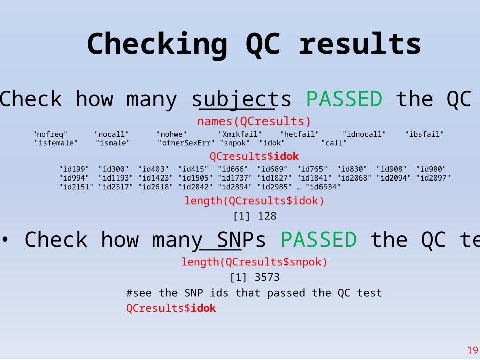
Checking QC results

• Check how many subjects PASSED the QC testnames(QCresults)

"nofreq" "nocall" "nohwe" "Xmrkfail" "hetfail" "idnocall" "ibsfail""isfemale" "ismale" "otherSexErr" "snpok" "idok" "call"

QCresults$idok"id199" "id300" "id403" "id415" "id666" "id689" "id765" "id830" "id908" "id980""id994" "id1193" "id1423" "id1505" "id1737" "id1827" "id1841" "id2068" "id2094" "id2097""id2151" "id2317" "id2618" "id2842" "id2894" "id2985" … "id6934“

length(QCresults$idok)

[1] 128

• Check how many SNPs PASSED the QC testlength(QCresults$snpok)

[1] 3573

#see the SNP ids that passed the QC test

QCresults$idok

19

56

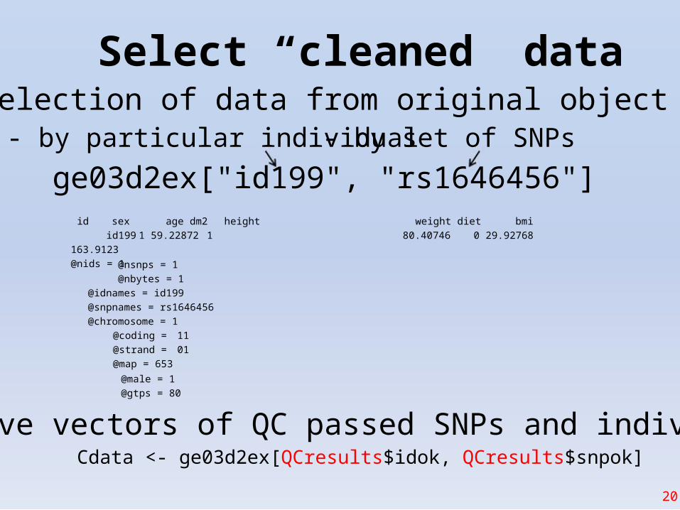
Select “cleaned” data• Selection of data from original object BOTH:

- by particular individual - by set of SNPs

ge03d2ex["id199", "rs1646456"]id sex age dm2 height

id199 1 59.22872 1

163.9123

@nids = 1@nsnps = 1

@nbytes = 1

@idnames = id199

@snpnames = rs1646456

@chromosome = 1

@coding = 11

@strand = 01

@map = 653

@male = 1

@gtps = 80

weight diet bmi

80.40746 0 29.92768

• Give vectors of QC passed SNPs and individualsCdata <- ge03d2ex[QCresults$idok, QCresults$snpok]

20

57

Check the quality of overall QC datadescriptives.marker(Cdata)

$`Minor allele frequency distribution`

X<=0.01 0.01<X<=0.05 0.05<X<=0.1 0.1<X<=0.2 X>0.2

No 0 508.000 677.000 873.000 1515.000

Prop 0 0.142 0.189 0.244 0.424

$`Cumulative distr. of number of SNPs out of HWE, at different alpha`

X<=1e-04 X<=0.001 X<=0.01 X<=0.05 all XNo 44.000 66.000 117.000 239.000 3573

Better but still lots of HWEoutliers. Population structure

not accounted for?

Prop 0.012 0.018 0.033 0.067 1

$`Distribution of proportion of successful genotypes (per person)`

X<=0.9 0.9<X<=0.95 0.95<X<=0.98 0.98<X<=0.99 X>0.99No 0 0 0 65.000 63.000

Prop 0 0 0 0.508 0.492

$`Distribution of proportion of successful genotypes (per SNP)`

X<=0.9 0.9<X<=0.95 0.95<X<=0.98 0.98<X<=0.99 X>0.99No 0 0 458.000 814.000 2301.000

Prop 0 0 0.128 0.228 0.644

The lambda did not improvedsignificantly also indicating that the QCdata still has factors not accounted for

estlambda(summary(Cdata)[,"Pexact"])

$estimate[1] 2.150531

$`Mean heterozygosity for a SNP`

[1] 0.2787418

$`Standard deviation of the mean heterozygosity for a SNP`

[1] 0.1497257

$`Mean heterozygosity for a person`

[1] 0.26521

$`Standard deviation of mean heterozygosity for a person`

[1] 0.01888496

The genotype data has muchhigher call rates since individualswith NA values eliminated in therange of > 99%

21

58

Which sub-group causing deviation from HWE?

descriptives.marker(Cdata[Cdata@phdata$dm2==0,])[2]$`Cumulative distr. of number of SNPs out of HWE, atdifferent alpha`

X<=1e-04 X<=0.001 X<=0.01 X<=0.05 all X

No 0 0 7.000 91.000 3573

Prop 0 0 0.002 0.025 1

descriptives.marker(Cdata[Cdata@phdata$dm2==1,])[2]

$`Cumulative distr. of number of SNPs out of HWE, atdifferent alpha`

X<=1e-04 X<=0.001 X<=0.01 X<=0.05

all X

No 46.000 70.00127.000228.000 3573Prop 0.013 0.02 0.036 0.064 1

As expected, the casesdisplay the greatestdeviation from HWE

controls

cases

22

59

Compare raw and cleaned data

plot(qTest, df="Pc1df", col="blue")

qTest_QC = qtscore(dm2,Cdata,trait="binomial")add.plot(qTest_QC , df="Pc1df", col="red")

Note that the cleaned data values are all lower this is due to lower λ value 23

60

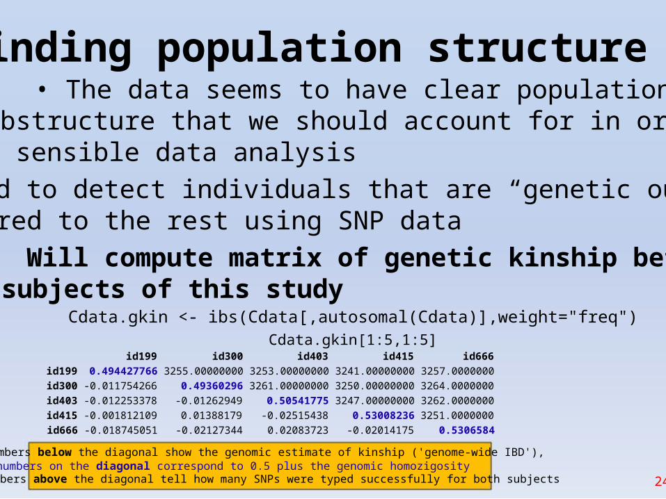
Finding population structure (1)• The data seems to have clear population

substructure that we should account for in order todo sensible data analysis

• Need to detect individuals that are “genetic outliers”compared to the rest using SNP data

1. Will compute matrix of genetic kinship betweensubjects of this study

Cdata.gkin <- ibs(Cdata[,autosomal(Cdata)],weight="freq")Cdata.gkin[1:5,1:5]

id199 id300 id403 id415 id666id199 0.494427766 3255.00000000 3253.00000000 3241.00000000 3257.0000000id300 -0.011754266 0.49360296 3261.00000000 3250.00000000 3264.0000000id403 -0.012253378 -0.01262949 0.50541775 3247.00000000 3262.0000000id415 -0.001812109 0.01388179 -0.02515438 0.53008236 3251.0000000

id666 -0.018745051 -0.02127344 0.02083723 -0.02014175 0.5306584

The numbers below the diagonal show the genomic estimate of kinship ('genome-wide IBD'),The numbers on the diagonal correspond to 0.5 plus the genomic homozigosityThe numbers above the diagonal tell how many SNPs were typed successfully for both subjects 24

61

Finding population structure (2)2. Compute distance matrix from previous

Cdata.dist <- as.dist(0.5-Cdata.gkin)

3. Do Classical Multidimensional Scaling (PCA)and visualize results

Cdata.mds <- cmdscale(Cdata.dist)plot(Cdata.mds)

• The PCA fitted thegenetic distances along

Outliers to exclude(Individuals)

the 2 components• Points are individuals• There are clearly two

clusters• Need to select all

individuals from biggestcluster

Component 1 25

62

Second round of QC• Select the ids of individuals from each cluster

- Can use k-means since clusters are well definedkmeans.res <- kmeans(Cdata.mds,centers=2,nstart=1000)

cluster1 <- names(which(kmeans.res$cluster==1))

cluster2 <- names(which(kmeans.res$cluster==2))

• Select another clean dataset using data forindividuals in cluster #2 (the largest)

Cdata2 <- Cdata[cluster2,]

• Perform QC on new dataQCdata2 <- check.marker(Cdata2, hweids=(phdata(Cdata2)$dm == 0), fdr = 0.2)

26

63

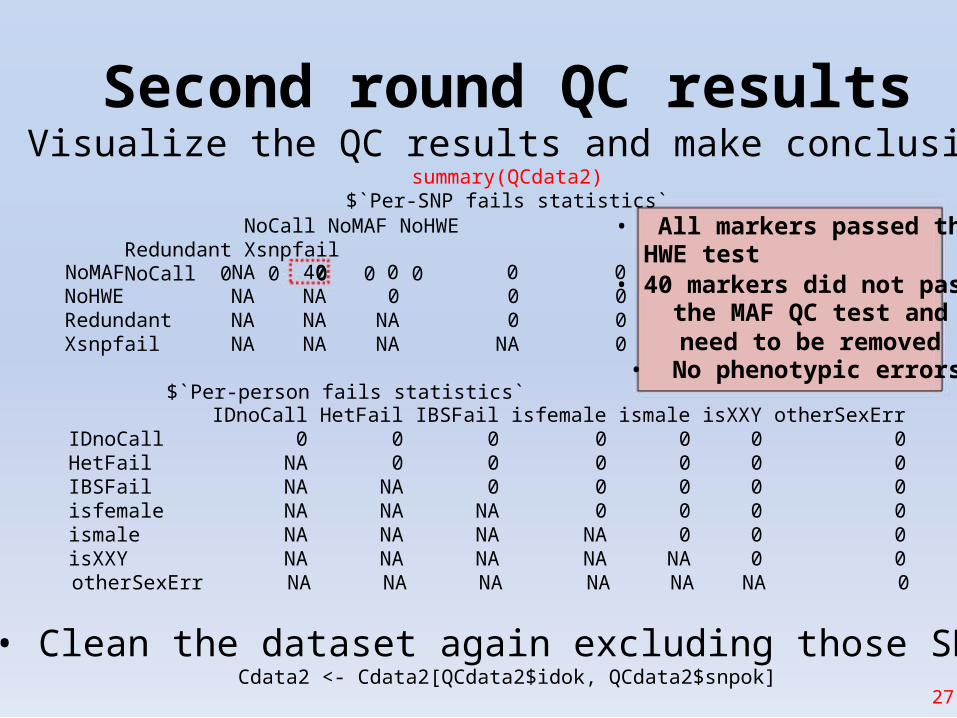
Second round QC results• Visualize the QC results and make conclusions

summary(QCdata2)$`Per-SNP fails statistics`

NoCall NoMAF NoHWE Redundant XsnpfailNoCall 0 0 0 0 0NoMAF NA 40 0 0 0

NoHWE NA NA 0 0 0Redundant NA NA NA 0 0Xsnpfail NA NA NA NA 0

$`Per-person fails statistics`

• All markers passed theHWE test

• 40 markers did not passthe MAF QC test andneed to be removed

• No phenotypic errors

IDnoCall HetFail IBSFail isfemale ismale isXXY otherSexErrIDnoCall 0 0 0 0 0 0 0HetFail NA 0 0 0 0 0 0IBSFail NA NA 0 0 0 0 0isfemale NA NA NA 0 0 0 0ismale NA NA NA NA 0 0 0isXXY NA NA NA NA NA 0 0otherSexErr NA NA NA NA NA NA 0

• Clean the dataset again excluding those SNPsCdata2 <- Cdata2[QCdata2$idok, QCdata2$snpok]

27

64

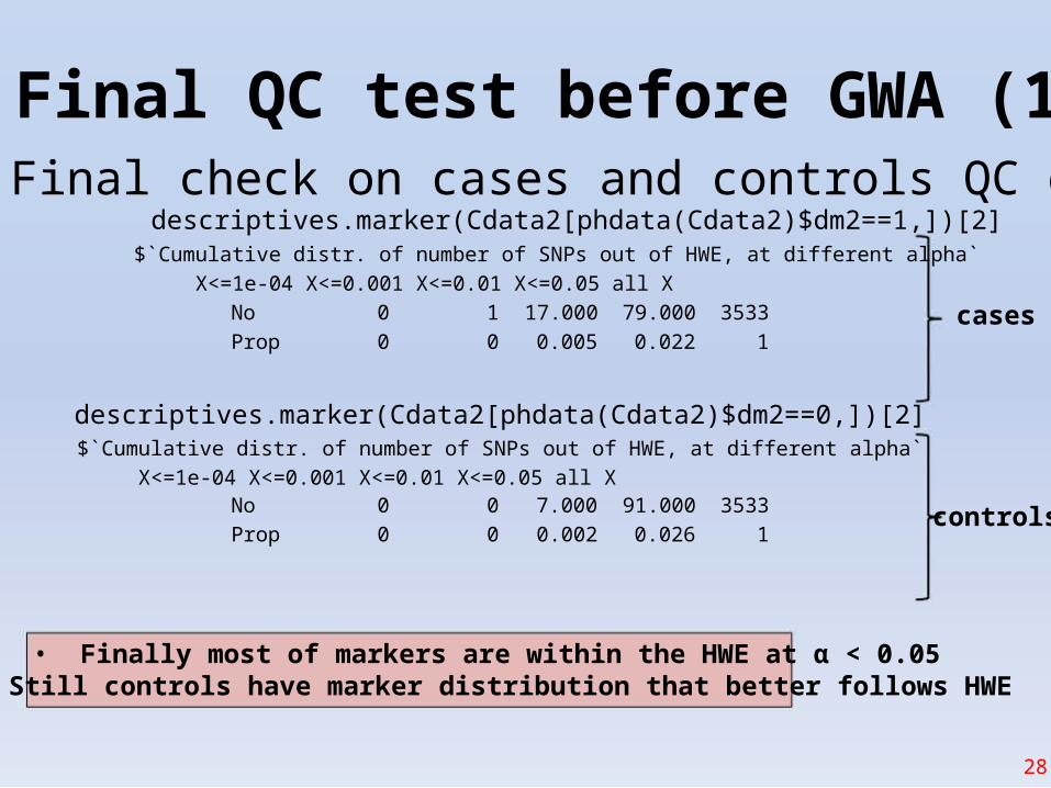
Final QC test before GWA (1)• Final check on cases and controls QC datadescriptives.marker(Cdata2[phdata(Cdata2)$dm2==1,])[2]

$`Cumulative distr. of number of SNPs out of HWE, at different alpha`

X<=1e-04 X<=0.001 X<=0.01 X<=0.05 all X

No 0 1 17.000 79.000 3533

Prop 0 0 0.005 0.022 1

descriptives.marker(Cdata2[phdata(Cdata2)$dm2==0,])[2]$`Cumulative distr. of number of SNPs out of HWE, at different alpha`

X<=1e-04 X<=0.001 X<=0.01 X<=0.05 all XNo 0 0 7.000 91.000 3533

Prop 0 0 0.002 0.026 1

• Finally most of markers are within the HWE at α < 0.05• Still controls have marker distribution that better follows HWE

cases

controls

28

65

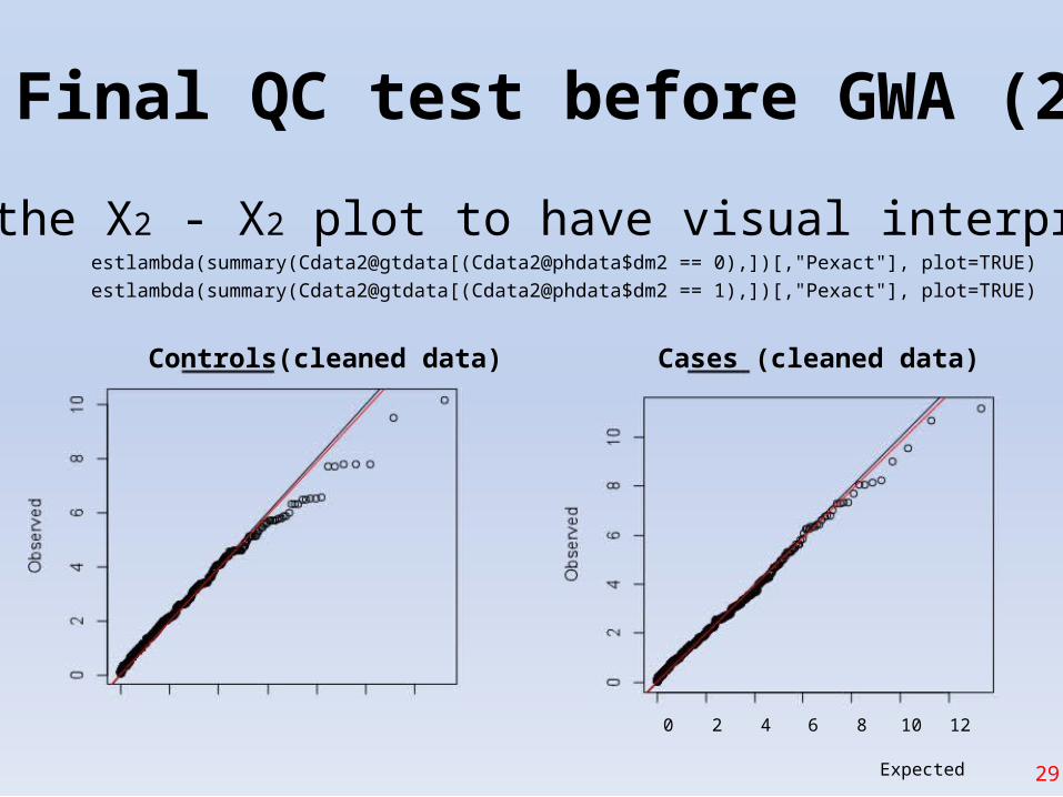
Final QC test before GWA (2)

• Do the X2 - X2 plot to have visual interpretationestlambda(summary(Cdata2@gtdata[(Cdata2@phdata$dm2 == 0),])[,"Pexact"], plot=TRUE)

estlambda(summary(Cdata2@gtdata[(Cdata2@phdata$dm2 == 1),])[,"Pexact"], plot=TRUE)

Controls(cleaned data) Cases (cleaned data)

0 2 4 6 8 10 12

Expected 29

66

Perform GWA on new data

• Perform the mixture model regression analysisCdata2.qt <- qtscore(Cdata2@phdata$dm2, Cdata2,trait="binomial")

descriptives.scan(Cdata2.qt,sort="Pc1df")

Summary for top 10 results, sorted by Pc1dfChromosome Position Strand A1 A2 N effB se_effB chi2.1df P1df effAB effBB chi2.2df P2df Pc1df

rs1719133 1 4495479 + T A 124 0.3167801 0.08614528 13.522368 0.0002357368 0.3740771 0.0000000 14.677906 0.0006497303 0.0003048399

rs4804634 1 2807417 + C G 121 0.4119844 0.12480696 10.896423 0.0009635013 0.6315789 0.1739130 12.375590 0.0020543516 0.0011885463rs8835506 2 6010852 + A T 121 3.5378209 1.08954331 10.543448 0.0011660066 4.0185185 4.0185185 12.605556 0.0018312105 0.0014292471

rs4534929 1 4474374 + C G 123 0.4547151 0.14160410 10.311626 0.0013219476 0.4830918 0.1739130 10.510272 0.0052206352 0.0016136479rs1013473 1 4487262 + A T 124 2.7839368 0.86860745 10.272393 0.0013503553 3.0495868 5.8441558 10.926296 0.0042401869 0.0016471605

rs3925525 2 6008501 + C G 124 3.2807631 1.03380675 10.070964 0.0015062424 3.6923077 4.0000000 11.765985 0.0027864347 0.0018306610rs3224311 2 6009769 + G C 124 3.2807631 1.03380675 10.070964 0.0015062424 3.6923077 4.0000000 11.765985 0.0027864347 0.0018306610

rs2975760 3 10518480 + A T 123 3.1802120 1.00916993 9.930784 0.0016253728 3.0000000 8.0000000 10.172522 0.0061810866 0.0019704699rs2521089 3 10487652 - T C 123 2.7298775 0.87761175 9.675679 0.0018672326 3.0147059 5.0000000 10.543296 0.0051351403 0.0022533033

rs1048031 1 4485591 + G T 122 0.4510793 0.14548378 9.613391 0.0019316360 0.4844720 0.1714286 9.965696 0.0068545128 0.0023284084

• Compare results to the previous QC round 1 results

30

67

Manhattan plots• Compare results QC round 1 vs QC round 2

plot(Cdata2.qt)

add.plot(qTest_QC, col="orange")Round 1 QCRound 2 QC

(accounted for populationstratification effects)

31

68

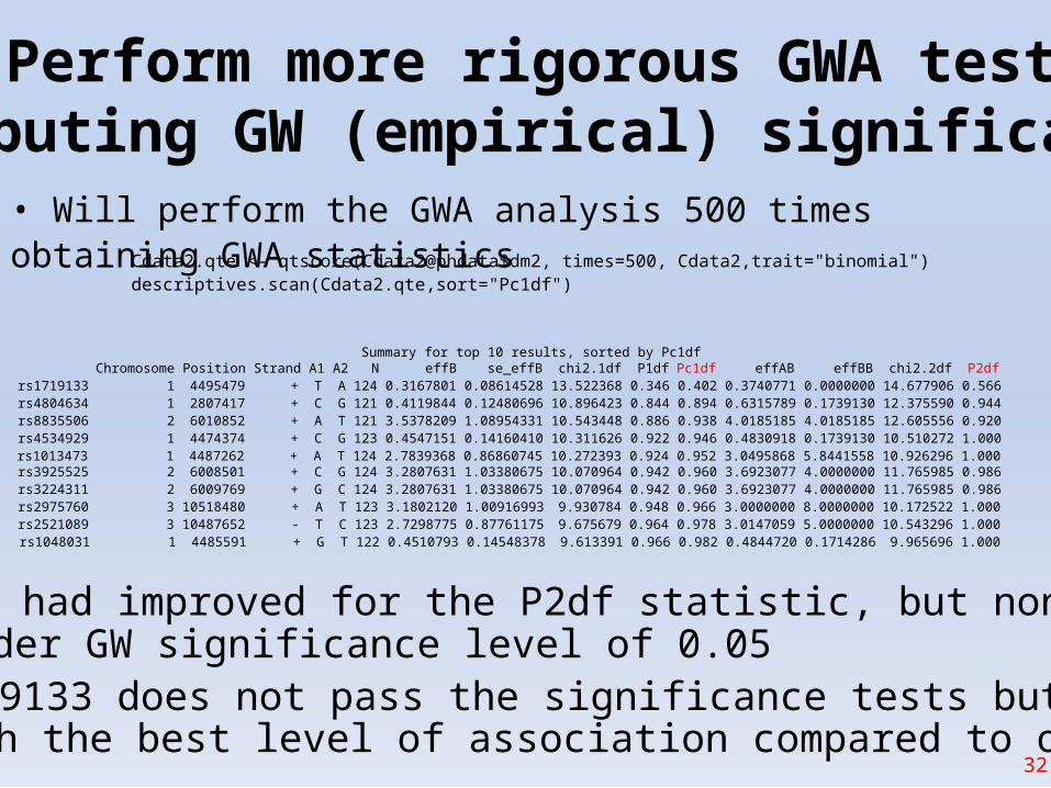
Perform more rigorous GWA testcomputing GW (empirical) significance

• Will perform the GWA analysis 500 times obtaining GWA statisticsCdata2.qte <- qtscore(Cdata2@phdata$dm2, times=500, Cdata2,trait="binomial")descriptives.scan(Cdata2.qte,sort="Pc1df")

Summary for top 10 results, sorted by Pc1dfChromosome Position Strand A1 A2 N effB se_effB chi2.1df P1df Pc1df effAB effBB chi2.2df P2df

rs1719133 1 4495479 + T A 124 0.3167801 0.08614528 13.522368 0.346 0.402 0.3740771 0.0000000 14.677906 0.566rs4804634 1 2807417 + C G 121 0.4119844 0.12480696 10.896423 0.844 0.894 0.6315789 0.1739130 12.375590 0.944rs8835506 2 6010852 + A T 121 3.5378209 1.08954331 10.543448 0.886 0.938 4.0185185 4.0185185 12.605556 0.920rs4534929 1 4474374 + C G 123 0.4547151 0.14160410 10.311626 0.922 0.946 0.4830918 0.1739130 10.510272 1.000rs1013473 1 4487262 + A T 124 2.7839368 0.86860745 10.272393 0.924 0.952 3.0495868 5.8441558 10.926296 1.000rs3925525 2 6008501 + C G 124 3.2807631 1.03380675 10.070964 0.942 0.960 3.6923077 4.0000000 11.765985 0.986rs3224311 2 6009769 + G C 124 3.2807631 1.03380675 10.070964 0.942 0.960 3.6923077 4.0000000 11.765985 0.986rs2975760 3 10518480 + A T 123 3.1802120 1.00916993 9.930784 0.948 0.966 3.0000000 8.0000000 10.172522 1.000rs2521089 3 10487652 - T C 123 2.7298775 0.87761175 9.675679 0.964 0.978 3.0147059 5.0000000 10.543296 1.000rs1048031 1 4485591 + G T 122 0.4510793 0.14548378 9.613391 0.966 0.982 0.4844720 0.1714286 9.965696 1.000

• Results had improved for the P2df statistic, but none of themfall under GW significance level of 0.05

• rs1719133 does not pass the significance tests but is theone with the best level of association compared to other SNPs

32

69

Biological interpretations• For illustration purposes let’s extract information on the rs1719133

from dbSNP• Seems to target CCL3 - pro-inflamatory cytokine. The CCL2 was

implicated in T1D [1]

70

Conclusions

• GWA studies are popular these days mainly due to high throughput technology development such as genotyping chips (i.e. SNP arrays) and sequences

• Analysis of GW data requires several steps ofquality control in order to draw conclusions

• GenABEL provides tools to perform GWAs and automate some of the steps

34

71

References[1] Ruili Guan et al. Chemokine (C-C Motif) Ligand 2 (CCL2) in Sera of Patients with Type 1Diabetes and Diabetic Complications. PLoS ONE 6(4): e17822[2] Yurii Aulchenko, GenABEL tutorial http://www.genabel.org/sites/default/files/pdfs/GenABEL-tutorial.pdf[3] GenABEL project developers, GenABEL: genome-wide SNP association analysis 2012, Rpackage version 1.7-2[4] Geraldine M Clarke et.al. Basic statistical analysis in genetic case-control studies. Nat Protoc. 2011 February ; 6(2): 121–133[5] Lobo, I. Same genetic mutation, different genetic disease phenotype. Nature Education 2008, 1(1)